Arnold maps with noise: Differentiability and non-monotonicity of the rotation number

Abstract.

Arnold’s standard circle maps are widely used to study the quasi-periodic route to chaos and other phenomena associated with nonlinear dynamics in the presence of two rationally unrelated periodicities. In particular, the El Niño–Southern Oscillation (ENSO) phenomenon is a crucial component of climate variability on interannual time scales and it is dominated by the seasonal cycle, on the one hand, and an intrinsic oscillatory instability with a period of a few years, on the other. The role of meteorological phenomena on much shorter time scales, such as westerly wind bursts, has also been recognized and modeled as additive noise.

We consider herein Arnold maps with additive, uniformly distributed noise. When the map’s nonlinear term, scaled by the parameter $\epsilon$, is sufficiently small, i.e. $\epsilon<1$, the map is known to be a diffeomorphism and the rotation number $\rho_{\omega}$ is a differentiable function of the driving frequency $\omega$.

We concentrate on the rotation number’s behavior as the nonlinearity becomes large, and show rigorously that $\rho_{\omega}$ is a differentiable function of $\omega$, even for $\epsilon\geq 1$, at every point at which the noise-perturbed map is mixing. We also provide a formula for the derivative of the rotation number. The reasoning relies on linear-response theory and a computer-aided proof. In the diffeomorphism case of  $\epsilon<1$, the rotation number $\rho_{\omega}$ behaves monotonically with respect to $\omega$. We show, using again a computer-aided proof, that this is not the case when $\epsilon\geq 1$ and the map is not a diffeomorphism. This lack of monotonicity for large nonlinearity could be of interest in some applications. For instance, when the devil’s staircase $\rho=\rho(\omega)$ loses its monotonicity, frequency locking to the same periodicity could occur for non-contiguous parameter values that might even lie relatively far apart from each other.

1. Introduction and motivation

The motivation of the present work is to provide further physical and mathematical insights into the behavior of the El Niño–Southern Oscillation (ENSO) phenomenon. ENSO is a dominant component of the climate system’s variability on the time scale of several seasons to several years [58, 62] and its accurate prediction for 6–12 months ahead is of great socio-economic importance [17, 35, 53].

Arnold map with noise as a climate toy model. The model studied herein is a highly idealized one that captures, however, two key features of interest of the ENSO phenomenon, namely frequency locking and high irregularity. Frequency-locking behavior has been observed in many fields of physics in general [9, 10, 26] and in several ENSO models in particular [21, 37, 45, 46, 65, 69, 70]. For instance, some early coupled ocean–atmosphere models that attempted to simulate and predict ENSO were locked into a two-year or a three-year cycle. Clearly, it is difficult to predict large El Niño events in the Eastern Tropical Pacific — which occur irregularly, every 2–7 years — with a model that has a persistent, stable periodicity of two or three years [36].

Frequency-locking, also called mode-locking, is due to nonlinear interaction between an internal frequency $\omega_{\mathrm{i}}$ of the system and an external frequency $\omega_{\mathrm{e}}$. In the ENSO case, the external periodicity is the seasonal cycle, while the internal periodicity is associated with an oscillatory instability that has been studied extensively in the absence of the seasonal cycle [58, and references therein]. A simple model for systems with two competing periodicities is the well-known standard circle map [4]. This map is often called the Arnold map and it is given by Eq. (2) at the beginning of the next section.

Strong nonlinearity. The deterministic Arnold circle map $T_{\tau,\epsilon}:S^{1}\rightarrow S^{1}$ is defined by

(1) $$T_{\tau,\epsilon}(x):=x+\frac{2\pi}{\omega}-\dfrac{\epsilon}{2\pi}\sin(2\pi x)\mod 1\,.$$

In the absence of nonlinear effects ($\epsilon=0$) the behavior of the deterministic map in Eq. 1 is relatively simple: either the driving frequency $\omega$ is rational, $\omega=p/q$ with $(p,q)$ integers, and the dynamics is periodic with period $p$; or $\omega$ is irrational and the iterates {$X_{n}$} of the map fill the whole circle $S^{1}$ densely. For small nonlinearity, $\epsilon\ll 1$, narrow Arnold tongues develop out of each rational-periodicity point $(\omega=p/q,\epsilon=0)$. Each such tongue increases in width with increasing $\epsilon$, while the periodicity within it stays equal to $p$; see Fig. 1. As $\epsilon$ exceeds the value $1.0$, the Arnold tongues overlap, and chaotic behavior sets in [4].

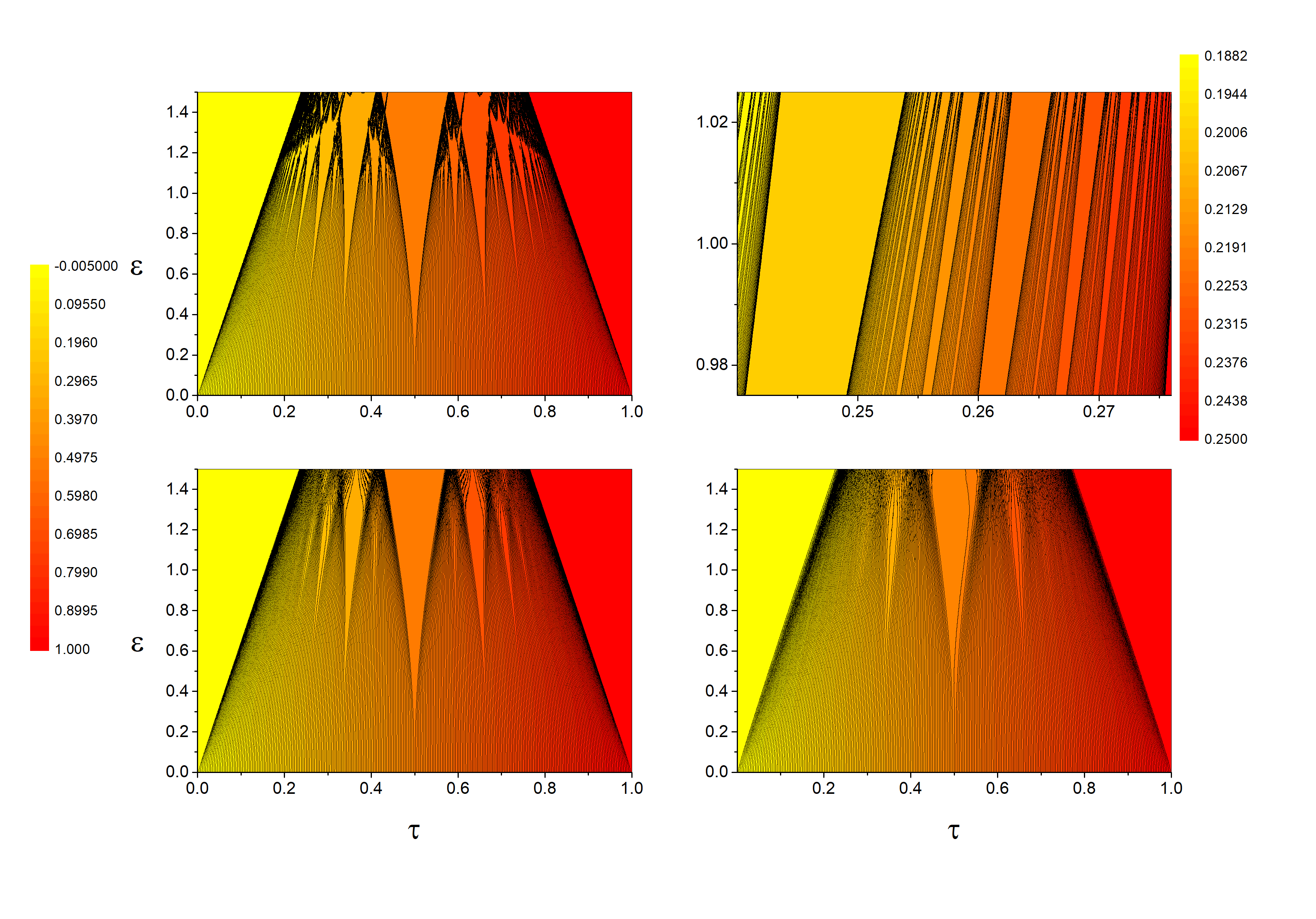
Figure 1. Contour maps of the  rotation number $\rho=\rho_{\tau}$ in the parameter space $(\tau,\epsilon)$, where $\tau=2\pi/\omega$. Each $\rho_{\tau}$ value was estimated by performing  10 000 iterations of the map  given by Eq. (2) in Section 2.1 below. Top panels: noise amplitude $\xi=0$, with a blow-up near the critical line $\epsilon=1$ at the right. Bottom panels: Noise amplitude $\xi=0.02$ (left) and $\xi=0.05$ (right). All numerical data were obtained for 4 000 values of $\tau$ and 200 of $\epsilon$, uniformly distributed in the corresponding intervals.

The observed irregular behavior of ENSO argues strongly for large nonlinearities being active and giving rise to chaotic behavior [33]. One such numerical result is illustrated by the “Devil’s bleachers” in Fig. 2.

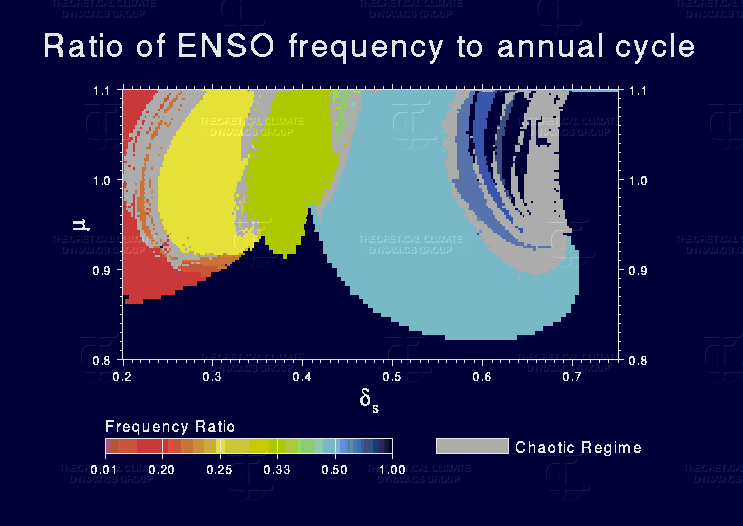
Figure 2. Devil’s bleachers from a relatively simple ENSO model based on the coupling of a partial differential equation for the ocean with an integral equation for the atmosphere [45, 46]. The two parameters are $\delta_{\mathrm{s}}$ on the abscissa and $\mu$ on the ordinate: $\delta_{\mathrm{s}}$ is a mixed ocean layer parameter that determines the periodicity of the internal oscillation, while $\mu$ corresponds to the strength of the local coupling between the atmosphere and ocean. The colors identify large areas of ENSO locking to 1–5 years, while gray identifies chaotic behavior; see color bar.  Courtesy of Fei-Fei Jin and based on numerical results of [46].

Noise sources in ENSO modeling. In climate modeling in general, variability on smaller scales in time and space is increasingly modeled as random. The so-called parametrization — i.e., large-scale representation of net effects — of subgrid-scale phenomena plays an increasing role in refining the most detailed and highly resolved climate models [59]. More specifically, the role of westerly wind bursts in the onset of El Niños has been studied more and more intensively [73]. These wind bursts over the western Tropical Pacific are at least correlated with and possibly causal to warm events in the eastern Tropical Pacific [25].

Timmermann and Jin [68] have included a stochastic process meant to represent these wind bursts into a low-order ENSO model and shown that it contributes to the irregular occurrence of the model’s warm events. This stochastically perturbed ENSO model has been further studied in [22], where its random attractor has been computed. Using an additive stochastic process in the toy model studied herein seems therewith amply justified.

In the present paper, we will formulate and apply techniques allowing one to obtain results on the rotation number of the strongly nonlinear Arnold circle map in the presence of additive noise. No claim is made that this results obtained herein could be applied directly to high-end climate models. It is common, though, in the climate sciences to deal with a full hierarchy of models [31, 41, 66]— from the Arnol’d circle map, through low-order systems of ordinary differential equations [54],[55], [44], [38], [61] and on to intermediate models governed by partial differential equations in one or two space dimensions, all the way to fully three-dimensional and highly detailed general circulation models. Moreover, it is more and more the case that the simulations of intermediate and high-end models are analyzed by data-driven methods to yield stochastic-dynamic models reproducing their main properties [60, 47]. It is to these models that advanced mathematical techniques, like the ones proposed in this paper, are then to be applied.

As we shall see forthwith, a key tool of our approach is linear response theory, which has already been applied fairly widely in the climate sciences ([52],[34],[40]). From the theoretical point of view linear response theory was proved to apply generally in random systems in which the presence of noise plays has a regulatizing effect ([40],[27]). We can expect, therefore, that several of the general ideas presented herein can be applied to low-order and intermediate climate models, in the presence of additive noise.

Linear response and stability of the statistical properties. In the following sections, we study the behavior of the statistical properties of Arnold maps with additive noise and strong nonlinearity. In particular, we study the behavior of their rotation number. We are interested in the smoothness of the rotation number $\rho$ as a function of the driving frequency $\omega$ and in its monotonicity properties. We will see that, in the strong nonlinearity case $\epsilon\geq 1$, $\rho=\rho(\omega)$ still varies smoothly, but it is not monotonic anymore, as it is in the weakly nonlinear case $\epsilon<1$.

Our findings rely both on general mathematical results and on rigorous computer-aided estimates. The smoothness of statistical properties of a family of dynamical systems is often guaranteed by the fact that its relevant stationary or invariant measure varies in a smooth way with respect to changes in a control parameter of the system. This property is called a linear response of the invariant measure under perturbation of the system. The system’s linear response with respect to a perturbation can be described by a suitable derivative, representing the rate of change of the relevant (physical, stationary) invariant measure of the system with respect to the perturbation.

The behavior of the stationary measure of a random or deterministic dynamical system under perturbations may be very different from system to system. Some classes of systems have a smooth behavior, with respect to suitable perturbations; this smoothness was proved for several classes of deterministic systems. Starting with the work of Ruelle (see [64]) which proved this for uniformly hyperbolic systems, similar results have been proved in some cases for non-uniformly expanding or hyperbolic ones (see e.g. [5, 11, 12, 13, 16, 23, 48, 77]). On the other hand, it is known that linear response does not always hold, due to the lack of regularity of the system or of the perturbation or to insufficient hyperbolicity; see [11, 15, 28, 77]. The survey paper [14] has an exhaustive list of classical references on the subject.

An example of linear response for small random perturbations of deterministic systems appears in [51]. Results for random systems were proved in [40], where the technical framework was adapted to stochastic differential equations and in [6], where the authors consider random compositions of expanding or non-uniformly expanding maps. Rigorous numerical approaches for the computation of the linear response are available, to some extent, both for deterministic and random systems (see [7, 63]).

In recent work [27], it was shown that, in the presence of additive noise, one can expect linear response, even for maps which are not expanding or hyperbolic. The Arnold maps with noise and strong nonlinearity and the kinds of perturbations we consider herein fit into this framework. In this paper, we will adapt the results of [27] to prove linear response for this class of systems and perturbations, along with smoothness of the rotation number. We remark that the results of [27] are not directly applicable to the kind of perturbations we need to consider here because these perturbations change the critical values of the deterministic part of the dynamics. In Section 3 we show how to deal with these perturbations.

Computer-aided estimates. Some of the results we present have been obtained with the help of computer-aided estimates. These estimates are obtained using suitable numerical software that tracks the possible truncation and numerical errors during the computation. The output of the computation is then an interval containing in a certified way the result that was meant to be estimated, e.g. “the rotation number $\rho$ of the given system is contained in the interval $[0.556,0.566]$”. Such rigorous computations can be implemented by suitable numerical methods and libraries, the results can be considered as statements proved by a computer-aided estimate; see, for instance, the book [71] for an introduction to the subject.

In this paper we will make use of the software and the methods developed in [29] for dynamical systems on the interval with additive noise.

The software will be used in this work for two purposes:

1. computing the stationary measure of a given Arnold map with noise to within a small, explicit error in the $L^{1}$-norm.

2. computing such a system’s mixing rate. The mixing rate is measured by the norm of the iterates of the transfer operator associated with the system, restricted to the space of measures having zero average on the phase space $S^{1}$.

Both of these computations are made possible by a kind of finite-element approximation of the transfer operator, used in combination with quantitative functional analytic stability statements that estimate explicitly, and not asymptotically the approximation errors made in the finite element reduction (as explained in [29]). Further details on this matter will be given in Sections 4.2 and 5, where we also show the results of the computer-aided estimates we use herein.

Plan of the paper. The paper is structured as follows:

In Section 2 we introduce the Arnold maps with noise that we study and the questions which are investigated in the paper. We also state informally the  paper’s main results.

In Section 3 we outline a general linear-response statement, and adapt it to the kind of systems and perturbations we investigate in the paper. This will be the core tool to show that the rotation number varies smoothly even in the strong nonlinear case $\epsilon\geq 1$.

The application of the theory built in Section 3 requires some quantitative estimate on the system’s mixing rate. In Section 4, we prove the quantitative stability results that are required to support a computer-aided estimation of the  system’s mixing rate and show the result of such computer-aided estimates.

Further computer-aided estimates in Section  5 yield rigorous non-monotonicity results for the rotation number in the strong nonlinearity case.

2. Mode locking in the presence of noise and our main results

In this section we introduce more precisely the systems and the problems being studied in the paper. We also state informally the main results of the paper and summarize the findings of the paper [78], which could be used to prove the smoothness of the rotation number in the weak nonlinearity case $\epsilon<1$, but cannot be used in the case $\epsilon\geq 1$.

2.1. Model formulation and questions investigated

The system we study is the stochastically perturbed Arnold circle map, where the usual, deterministic circle map $T_{\tau,\epsilon}:S^{1}\rightarrow S^{1}$ is defined by

(2) $$T_{\tau,\epsilon}(x):=x+\tau-\dfrac{\epsilon}{2\pi}\sin(2\pi x)\mod 1\,.$$

Here $\tau:=2\pi/\omega$ and $\omega:=\omega_{\mathrm{i}}/\omega_{\mathrm{e}}$  is the driving frequency, while $\epsilon\geq 0$ parameterizes the magnitude of nonlinear effects. In other situations, where external driving is replaced by genuine coupling between two oscillators, one also refers to $\epsilon$ as the coupling parameter.

By Arnold map with additive noise we mean the stochastic process $\{X_{n}\}_{n\in\mathbb{N}}$ on $S^{1}$ defined by

(3) $$X_{n+1}=T_{\tau,\epsilon}(X_{n})+\Omega_{n}\mod 1\,.$$

At each iterate of  $T_{\tau,\epsilon}(x)$, an independent identically distributed (i.i.d.) noise $\Omega_{n},$ that is uniformly distributed on $[-\xi/2,\xi/2],$ is added to the deterministic term on the right-hand side of (3); in particular, the noise is independent of the point $X_{n}\in S^{1}$.

In the case $\epsilon=0,\xi=0$, the system is simply a rotation of the circle. In the deterministic case, where $\xi=0$, and $\epsilon\in(0,1)$ we get the classical Arnold circle map, which is one of the simplest models of coupled oscillators [2, 42, 3, 39, 33]. Outside climate science, in the context of cardiac dynamics the circle map was employed as a model for cardiac arrhythmias [3, 39] in which the irregular dynamics of heart pumping is interpreted as arising from the competition of two pacemakers. Similar studies were carried out in neurophysiology to investigate the dynamical behavior of a neuron subject to periodic stimulation [42]. In addition, the Arnold circle map was recently used as a model of the sleep-wake regulation cycle [8]. In another study a chain of coupled Arnold circle maps was employed to study the emergence of phase-locking patterns as a function of the coupling [18].

In the deterministic case, one of the most striking feature of this model is the mode-locking phenomenon: let us consider the rotation number. The rotation number $\rho=\rho_{\tau}$ measures the average rotation per iterate of (2) on $S^{1}$ and is defined as

$$\rho_{\tau}:=\lim_{n\rightarrow\infty}\frac{\tilde{T}_{\tau,\epsilon}^{n}(x)}{n}$$

where $\tilde{T}_{\tau,\epsilon}^{n}:\mathbb{R\rightarrow R}$ is the lift of $T_{\tau,\epsilon}$ to $\mathbb{R}$, defined by

(4) $$\tilde{T}_{\tau,\epsilon}(x):=x+\tau-\frac{\epsilon}{2\pi}\sin(2\pi x).$$

In this case we consider a system with additive noise as in $($3$)$ we define the rotation number by considering a stochastic process $\tilde{X}$ on $\mathbb{R}$ defined by $\tilde{X}_{n+1}=\tilde{T}_{\tau,\epsilon}(\tilde{X}_{n})+\Omega_{n}$ and $\rho_{\tau}:=\lim_{n\rightarrow\infty}\frac{\tilde{X}_{n}}{n}$.

There are some general classical results concerning the properties of the rotation number for deterministic and orientation-preserving diffeomorphisms of the circle that is useful to recall here (further details can be found in [79, 80]): it is well known that the rotation number is independent of $x\in S^{1}.$ A very important result is the Denjoy theorem that states that an orientation-preserving diffeomorphism (for our maps $T_{\tau,\epsilon}$ this corresponds to the weakly nonlinear case $\epsilon<1$) having an irrational rotation number is topologically conjugate to an irrational rotation in $S^{1}$ (see [80, 75]). The mode locking corresponds to the fact that the rotation number is locally constant around rational values of the driving frequency $\tau$: the map ”rotation number vs driving frequency” is a devil’s staircase (see Fig. 3 for one example). Concerning the existence of the derivative of $\rho_{\tau}$, with respect to the parameter $\tau$ of an orientation-preserving diffeomorphism, a classical result asserts that this derivative is defined in a point $\tau_{0}$ when the corresponding rotation number is irrational ($\rho_{\tau_{0}}\not\in\mathbb{Q}$) [79]. Moreover, as shown recently in [81], when $\tau_{0}$ is the endpoint of an interval for which $\rho_{\tau_{0}}\in\mathbb{Q}$ then the following result holds $\lim_{\tau\rightarrow\tau_{0}}\sup\frac{\rho_{\tau}-\rho_{\tau_{0}}}{\tau-\tau_{0}}=\infty$. Hence in the diffeomorphism case, $\rho_{\tau}$ cannot increase differentiably as $\tau$ grows. Other results in this direction appear in [82].

In Fig. 3, we plot the behavior or the rotation number of the system with additive noise at each iterate like in (3). It is easy to notice that in this case, the graph of the rotation number seems to go through a ”smoothing” process, i.e the map $\tau\mapsto\rho_{\tau}$ becomes smooth. In the case of weak nonlinearity, $\epsilon\in(0,1),$ this was rigorously proved by the work of [78].  To the best of our knowledge, both in the deterministic case and in the case with additive noise, no rigorous results about the differentiability of $\rho_{\tau}$ are present in the literature for the case where $\epsilon\geq 1$.
In the present paper we focus to this case, where the methods of [78] cannot work; from the physical point of view this case corresponds to strong nonlinear behavior and from the mathematical point of view it corresponds to the fact that the map $T_{\tau,\epsilon}$ is not a diffeomorphism anymore.

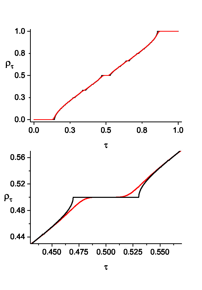
Figure 3. Plot of the rotation number $\rho=\rho_{\tau}$ for $\epsilon=0.9$. The black line corresponds to the absence of uniformly distributed noise, while the red line shows this dependence in the presence of such noise, with amplitude $\xi=0.05$. Recall that $\tau=2\pi/\omega$, where $\omega$ is the driving frequency. The lower panel is a blow-up of the dependence near the value $\tau=0.5$.

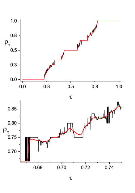
Figure 4. Same as Fig. 3 but for $\epsilon=1.4$ and for noise amplitude $\xi=0.01$. Here the lower panel is a blow-up of the dependence near $\tau=0.7$.

For $T_{\tau,\epsilon}$, when $\epsilon\geq 1$ a mode locking phenomenon can still be observed, but the behavior of the rotation number as a function of the driving frequency is more complicated. In Fig. 4 we show a plot of the rotation number both in the case with noise and without noise. We can observe that the action of the noise makes the rotation number smoother, as in the diffeomorphism case. Furthermore we can observe that the rotation number is not monotonic anymore as $\tau$ increases. This happens both with noise and without noise. The goal of this paper is to propose an explanation for those observations in the presence of noise, at the crossroads of linear response theory and computer-assisted proofs.

More precisely, we prove that :

a):

The rotation number is differentiable even in the case $\epsilon\geq 1$ at every value for the parameter $\tau$ for which the system is mixing and we provide examples of intervals for which this assumption is satisfied (see Section 4.2). We also provide an explicit formula to compute the derivative.

This will be done adapting some general linear response results for systems with noise coming from [27]. In those results the mixing assumption is needed. We verify the assumption with some certified computer aided estimates, establishing that the system is mixing when $\tau$ is in certain intervals.

b):

The rotation number is not always monotonic. In particular we show intervals for which there is a decreasing of the rotation number. (see Section 5).

This will be done by a certified approximation of the rotation number for a certain values of the parameters. The certified estimate on the rotation number will come from a certified approximation of the stationary measure of the system with a small error in $L^{1}$, using the framework developed in [29].

We emphasize that the tools we develop here are only suitable to study this problem in the presence of noise. More precisely, we can study the influence of changes in the driving frequency $\tau$, or in the noise amplitude $\xi$ (although we do not write it here, see [27, §4.2]), as long as it does not go to $0$. The approach here used is adapted to systems which are fastly converging to equilibrium and this is granted in our examples by the presence of noise.

3. Differentiability of the rotation number  for strong nonlinearity

In this section, we show that when the system is mixing, cf. Assumption LR1 of Theorem 8, there is linear response and the rotation number is differentiable with respect to changes in the parameter $\tau$.  This important inference will be obtained by adapting general linear response results for systems with additive noise to our case. In the following section, we start to introduce these results and the preliminary functional analytic work that is necessary.

The theoretical work will lead to linear response statements for families of Arnold maps with noise, in which the forcing parameter $\tau$ is modulated. The linear response will, in turn, lead to the differentiability of the associated rotation number; see Proposition 16 and Corollary 18.

3.1. Linear response for  mixing systems with additive noise

Let $BS(S^{1})$ be the set of Borel signed measures on $S^{1}$. This is a normed vector space if we consider the Wasserstein-Kantorovich norm defined on $BS$ as

(5) $$\|\mu\|_{W}=\underset{\|g\|_{\infty}\leq 1,~{}Lip(g)\leq 1}{\sup}\int_{S^{1}}g(x)d\mu.$$

where $Lip(g)$ is the best Lipschitz constant of $g$. We remark that $BS$ is not complete with this norm. The completion leads to a distributions space that is the dual of the space of Lipschitz functions.
We recall the following classic fact: the subspace spanned by Dirac masses in $BS$ is dense for the weak-$\star$ topology. Notice also that in this topology, one may approximate Dirac masses by multiples of indicators functions (e.g $\dfrac{1}{2\epsilon}\mathds{1}_{(a-\epsilon,a+\epsilon)}$ goes to $\delta_{a}$, the Dirac mass at $a\in S^{1}$, when $\epsilon\to 0$, in the weak-$\star$ topology). Thus, one may approximate any Borel signed measure by a $L^{1}$ function in the weak-$\star$ topology. As the unit ball of the space of Lipschitz functions is compact in $C^{0}(S^{1})$, it follows that one may approximate any Borel signed measure by a $L^{1}$ function in the Wasserstein norm.

We remark that since $S^{1}=\mathbb{R}/\mathbb{Z}$ is an additive group endowed with a Haar-Lebesgue measure (here denoted by $m$), there is a well defined notion of convolution. More precisely, given $f,g\in L^{1}((S^{1},m),\mathbb{R)}$ let us define the convolution $f\ast g$ as

$$f\ast g(t)=\int_{\mathbb{S}^{1}}f(t-\tau)g(\tau)d\tau.$$

It is easy to see that $f\ast g$ is a $L^{1}((S^{1},m),\mathbb{R})$ function, and that the convolution $\ast$ is commutative. In this context, it is also possible to define the convolution of two signed measures $f,g\in BS(S^{1})$, $f\ast g\in BS(S^{1})$ as the Borel signed measure

$$f\ast g(A):=\int_{S^{1}}\int_{S^{1}}\mathds{1}_{A}(x+y)df(x)dg(y).$$

There is a particularly useful special case of the convolution of two measures in $BS(S^{1})$: suppose $f$ is absolutely continuous with respect to $m$. In this case we have

$$f\ast g(t)=\int_{\mathbb{S}^{1}}f(t-\tau)dg(\tau).$$

It is noteworthy that in this case the convolution $f\ast g$ is a $L^{1}(m)$ function: this is a first instance of the regularization properties of the convolution, which we highlight and develop in the next section.

Remark 1.

When dealing with measures which are absolutely continuous with respect to the Lebesgue measure we will often identify the measure itself with his $L^{1}$density, to simplify notations.

We end by recalling the definition of variation for a signed measure and a function.

Definition 2.

Let $g$ be a finite Borel measure with sign on $S^{1}$. Given its decomposition as the difference of two positive measures $g=g^{+}+g^{-}$, we define its total variation as

$$\|g\|=g^{+}(S^{1})+g^{-}(S^{1}).$$

Let $f\in L^{1}(S^{1},m)$ be the density of an absolutely continuous measure and $P=P(x_{1},x_{2},\ldots,x_{n})$ be the set of endpoints of a finite partition of $S^{1}$. Let us denote $x_{0}:=x_{n}$. We define the variation of $f$ with respect to $P$ as

(6) $$Var_{P}(f):=\sum_{k=1}^{n}|f(x_{k})-f(x_{k-1})|.$$

If there exists $M$ such that $Var(f):=\underset{P}{\sup}\ Var_{P}\leq M$, with $P\in\{finite~{}partitions\}$, then $f$ is said to be of Bounded Variation. Let the Banach space of Borel measures having a bounded variation density be denoted as

$$BV(S^{1})=\{f\in L^{1},Var(f)<\infty\}$$

with the norm $\|f\|_{BV}=\|f||_{L^{1}}+Var(f)$. We will always use $BV$ for $BV(S^{1})$ unless $BV(\cdot)$ specifies an argument for the space.

3.1.1. Regularization estimates

The next lemmas provide regularization properties of the convolution that will be used later.

Lemma 3.

Let $f\in L^{1}(m)$ and $g\in BS(S^{1})$.  The following inequality holds:

$$\|f\ast g||_{L^{1}}\leq\|g\|\cdot\|f||_{L^{1}}.$$

Proof.

Suppose first that $g$ is positive

$$\|f\ast g||_{L^{1}} \leq \underset{\|h\|_{\infty}\leq 1}{\sup}\left|\int_{\mathbb{S}^{1}}h(t)~{}(f\ast g)(t)dt\right|$$

$$= \underset{\|h\|_{\infty}\leq 1}{\sup}\left|\int_{\mathbb{S}^{1}}h(t)\int_{\mathbb{S}^{1}}f(t-\tau)dg(\tau)\,dt\right|$$

$$\leq \underset{\|h\|_{\infty}\leq 1}{\sup}\left|\int_{\mathbb{S}^{1}}\int_{\mathbb{S}^{1}}h(t)f(t-\tau)dt~{}dg\right|\,$$

$$\leq \int_{\mathbb{S}^{1}}\|f\|_{L^{1}}~{}dg(\tau)\leq\|f\|_{L^{1}}\cdot g(S^{1}).$$

The general case follows by the linearity of the convolution considering $g=g^{+}-g^{-}$ and the fact that $g^{-},g^{+}$ are positive measures.    

Lemma 4.

Let $f\in BS[S^{1}]$ and $g\in L^{1}(S^{1})$. We have

(7) $$\|f\ast g\|_{W}\leq\|f\|_{W}\cdot\|g||_{L^{1}}.$$

Proof.

Let us consider $f\in BS(S^{1})$ and $g\in L^{1}(S^{1})$. Let $h\in Lip(S^{1})$ be such that $\|h\|_{\infty}+Lip(h)\leq 1$.
To prove (7), we estimate the quantity

$$\left|\int_{S^{1}}h(z)d(f\ast g)(z)\right| =\left|\int_{S^{1}}\int_{S^{1}}h_{y}(x)df(x)g(y)dy\right|$$

$$\leq\int_{S^{1}}\left|\int_{S^{1}}h_{y}(x)df(x)\right||g(y)|dy$$

$$\leq\|f\|_{W}\|g||_{L^{1}}$$

where $h_{y}(x):=h(x+y)$ is also a Lipschitz function satisfying $\|h_{y}\|_{\infty}+Lip(h_{y})\leq 1$.
Thus we have

$$\|f\ast g\|_{W}:=\sup_{\QATOP{h\in Lip(S^{1})}{\|h\|_{Lip}\leq 1}}\left|\int_{S^{1}}h(z)d(f\ast g)(z)\right|\leq\|f\|_{W}\|g||_{L^{1}}$$

   

The next definition introduces the space of zero average measures.

Definition 5.

Let us define the space of zero average measures $V\subset L^{1}$ as

(8) $$V:=\{f\in L^{1}(S^{1})~{}s.t.~{}\int_{S^{1}}f~{}dm=0\}.$$

Lemma 6.

Let $f\in BS(S^{1})$ such that $f(S^{1})=0$ and $g\in BV$. Then the convolution $f\ast g\in L^{1}(S^{1})$ and

(9) $$\|f\ast g||_{L^{1}}\leq 2\|f\|_{W}\cdot\|g\|_{BV}.$$

Proof.

Consider a $C^{1}$ function $g_{\varepsilon}$ such that $\|g_{\varepsilon}-g||_{L^{1}}\leq\varepsilon$ and $\|g_{\varepsilon}\|_{BV}=\|g\|_{BV}$, then by Lemma 3

$$\|f\ast g-f\ast g_{\varepsilon}||_{L^{1}}\leq\varepsilon$$

thus we can replace $g$ with $g_{\varepsilon}$ up to an error which is as small as wanted in the estimate we consider. We now consider $\|f\ast g_{\varepsilon}||_{L^{1}}$. Since $g_{\varepsilon}$ is $C^{1}$ with compact support, it is bounded and has bounded derivative. Hence there is $C$ such that for every $f_{\epsilon}\in V$ satisfying $\|f_{\epsilon}-f\|_{W}\leq$ $C\epsilon$, it holds $|f\ast g_{\varepsilon}(x)-f_{\epsilon}\ast g_{\varepsilon}(x)|\leq\epsilon$ for every $x\in{\mathbb{R}}$, by which

$$\|f_{\epsilon}\ast g_{\epsilon}-f\ast g_{\varepsilon}||_{L^{1}}\leq\varepsilon$$

Thus we may also replace $f$ with $f_{\epsilon}$ in our main estimate. Remark that $f_{\epsilon}\ast g_{\varepsilon}(t)$ is a $C^{1}$ function, with $(f\ast g_{\varepsilon})^{\prime}=f\ast g_{\epsilon}^{\prime}$.
Let us consider

$$\hat{h}(t)=\left\{\begin{array}[]{c}\frac{|f_{\epsilon}\ast g_{\varepsilon}(t)|}{f_{\epsilon}\ast g_{\varepsilon}(t)}~{}\mathrm{if}~{}(f_{\epsilon}\ast g_{\varepsilon})(t)\neq 0\\ 0~{}\mathrm{if}~{}(f_{\epsilon}\ast g_{\varepsilon})(t)=0\end{array}\right.$$

and

$$h(t)=\hat{h}(t)-\int\hat{h}(t)dt.$$

$\hat{h}$ is simply the sign function of $f_{\epsilon}\ast g_{\epsilon}$. Thus by definition of $\hat{h}$,

$$\|f_{\epsilon}\ast g_{\varepsilon}||_{L^{1}}=\int_{\mathbb{S}^{1}}\left|(f_{\epsilon}\ast g_{\varepsilon})(t)\right|dt=\int_{S^{1}}h(t)(f_{\epsilon}\ast g_{\varepsilon})(t)dt.$$

Indeed, recalling that $f_{\epsilon}\ast g_{\varepsilon}\in V$

$$\int_{S^{1}}[\hat{h}(t)-\int_{S^{1}}\hat{h}dt](f_{\epsilon}\ast g_{\varepsilon})(t)dt = \int_{S^{1}}\hat{h}(t)(f_{\epsilon}\ast g_{\varepsilon})(t)dt$$

$$= \int_{\mathbb{S}^{1}}\left|(f_{\epsilon}\ast g_{\varepsilon})(t)\right|dt.$$

Taking a one-periodic representative of $f_{\epsilon}\ast g_{\epsilon}$, we can interpret the integral on $S^{1}$ as an integral on $[0,1]$. Since $h$ has zero average, its primitive $\int_{0}^{t}h(s)ds=k(t)$ is also a one-periodic map. Applying integration by parts thus yields:

$$\|f_{\epsilon}\ast g_{\varepsilon}||_{L^{1}}=\int_{0}^{1}\int_{0}^{t}h(r)dr~{}(f_{\epsilon}\ast g_{\varepsilon})^{\prime}(t)dt=\int_{0}^{1}k(t)(f_{\epsilon}\ast g_{\varepsilon}^{\prime})(t)dt.$$

Note that since its derivative $h$ is bounded by $2$, $k$ is a $2-$Lipschitz function on $S^{1}$.
The last integral can be rewritten as

$$\int_{0}^{1}k(t)\left(\int_{S^{1}}g_{\varepsilon}^{\prime}(t)f_{\epsilon}(t-s)ds\right)dt =\int_{S^{1}}\int_{S^{1}}k(t)g_{\varepsilon}^{\prime}(s)f_{\epsilon}(t-s)dsdt$$

$$=\int_{S^{1}}\int_{S^{1}}k(t)f_{\epsilon}(t-s)g_{\varepsilon}^{\prime}(s)dtds$$

$$=\int_{S^{1}}\left(\int_{S^{1}}k(t+s)f_{\epsilon}(t)dt\right)g_{\epsilon}^{\prime}(s)ds$$

by applying Fubini-Tonelli theorem. Thus we obtain

$$\|f_{\epsilon}\ast g_{\varepsilon}||_{L^{1}}\leq\int_{S^{1}}\left|\int_{S^{1}}k_{s}(t)f_{\epsilon}(t)dt\right||g_{\epsilon}^{\prime}(s)|ds\leq 2\|f_{\epsilon}\|_{W}\|g_{\epsilon}\|_{BV}$$

since $k_{s}:t\mapsto k(t+s)$ is a $2$-Lipschitz function satisfying $\|k_{s}\|_{\infty}\leq 2$ for all $s\in S^{1}$. This last estimate being valid for each $\varepsilon$, the proposition is established.    

Lemma 7.

Let $f\in L^{1},$ $g\in BV$

(10) $$\|f\ast g\|_{BV}\leq\|f||_{L^{1}}\cdot\|g\|_{BV}.$$

Proof.

Similar estimates are well known for the convolution on $\mathbb{R}$. We prove the estimate on $S^{1}.$ Let us suppose first that $f,g\in C^{1}(S^{1})$. In this case $f\ast g\in C^{1}$and

$$Var(f\ast g)=\int_{\mathbb{S}^{1}}\left|(f\ast g)^{\prime}(t)\right|dt=\int_{\mathbb{S}^{1}}\left|f\ast g^{\prime}(t)\right|dt$$

and by Lemma 3

$$Var(f\ast g)\leq\|f||_{L^{1}}\|g^{\prime}||_{L^{1}}$$

from which we get directly the statement.

Now suppose $f\in C^{1}$ and $g\in BV$, let us consider as before $g_{\varepsilon}\in C^{1}$ such that $\|g_{\varepsilon}-g||_{L^{1}}\leq\varepsilon$ and $\|g_{\varepsilon}\|_{BV}=\|g\|_{BV}.$

Now

$$Var(f\ast g) \leq Var(f\ast g-g_{\epsilon})+Var(f\ast g_{\epsilon})$$

$$\leq Var(f\ast g-g_{\epsilon})+\|f||_{L^{1}}\|g_{\epsilon}^{{}^{\prime}}||_{L^{1}}$$

but $Var(f\ast g-g_{\epsilon})\leq Var(f)\|g-g_{\epsilon}\|\leq\epsilon Var(f)$ and can be made as small as wanted, allowing to prove the statement in the case $f\in C^{1}$ and $g\in BV.$

Now by approximating $f\in L^{1}$ by a $f_{\varepsilon}\in C^{1}$ such that $\|f_{\varepsilon}-f||_{L^{1}}\leq\varepsilon$ and using again Lemma 3 we get the full statement.    

3.1.2. Linear response, a general statement.

In [27], systems with additive noise are considered and a linear response theorem is proved for a general class of Markov operators including dynamical systems with additive noise. We state the theorem and apply it to the random Arnold maps and perturbations we mean to consider.
We will consider a normed vector space $(B_{w},\|\cdot\|_{w})$, with $BS\supseteq B_{w}\supseteq L^{1}$ and $\|\cdot\|_{w}\leq\|\cdot||_{L^{1}}$, as well as its space of zero average measure $V_{w}$.

(11) $$V_{w}:=\{\mu\in B_{w}~{}s.t.~{}~{}\mu(S^{1})=0\}.$$

Let us consider a family of Markov operators $L_{\delta}:BS(S^{1})\rightarrow BS(S^{1})$, where $\delta\in[0,\overline{\delta})$.

Recall that a Markov operator $L$ is positive and preserves probability measures: if $f\geq 0$ then $Lf\geq 0$ and $f(S^{1})=Lf(S^{1})$ for each $f\in BS(S^{1})$. Let us denote by ${Id}$ the identity operator, and by $(z{Id}-L)^{-1}$ the resolvent related to an operator $L$, formally defined as

(12) $$(z{Id}-L)^{-1}=\sum_{n=0}^{\infty}\dfrac{1}{z^{n+1}}L^{n}.$$

which is rigorously defined on suitable spaces whenever the infinite series converges. Let us suppose that each operator $L_{\delta}$ has a fixed probability measure in $BV(S^{1})$. We now show that under mild further assumptions these fixed points vary smoothly in the weaker norm $\|\cdot\|_{w}$. The following general result on linear response for  system with additive noise is proved in [27].

Theorem 8.

Suppose that the family of operators $L_{\delta}$ satisfies the following  four conditions:

• $f_{\delta}\in BV(S^{1})$ is a probability measure such that $L_{\delta}f_{\delta}=f_{\delta}$ for each $\delta\in\left[0,\overline{\delta}\right)$. Moreover there is $M\geq 0$ such that $\|f_{\delta}\|_{BV}\leq M$ for each $\delta\in\left[0,\overline{\delta}\right)$.

• (mixing for the unperturbed operator) For each $g\in BV(S^{1})$ with ${\int g\,dm=0}$

  $$\lim_{n\rightarrow\infty}\|L_{0}^{n}g||_{L^{1}}=0.$$

• (regularization of the unperturbed operator) $L_{0}$ is regularizing from $B_{w}$ to $L^{1}$ and from $L^{1}$ to Bounded Variation i.e. $L_{0}:(B_{w},\|\cdot\|_{w})\rightarrow L^{1}$ , ${\ L_{0}:L^{1}\rightarrow BV}$ are continuous.

• (small perturbation and derivative operator) There is $K\geq 0$ such that $\left||L_{0}-L_{\delta}|\right|_{L^{1}\rightarrow(B_{w},\|\cdot\|_{w})}\leq K\delta,$ and $\left||L_{0}-L_{\delta}|\right|_{BV\rightarrow V}\leq K\delta$. There is ${\dot{L}f_{0}\in V_{w}}$ such that

  (13) $$\underset{\delta\rightarrow 0}{\lim}\left\|\frac{(L_{0}-L_{\delta})}{\delta}f_{0}-\dot{L}f_{0}\right\|_{w}=0.$$

Then $({Id}-L_{0})^{-1}:V_{w}\rightarrow$ $V_{w}$ is a continuous operator and we have the following linear response formula

(14) $$\lim_{\delta\rightarrow 0}\left\|\frac{f_{\delta}-f_{0}}{\delta}-({Id}-L_{0})^{-1}\dot{L}f_{0}\right\|_{w}=0.$$

Thus $({Id}-L_{0})^{-1}\dot{L}f_{0}$ represents the first-order term in the change of equilibrium measure for the family of systems $L_{\delta}$.

Remark 9.

Condition LR0 is always satisfied by systems with additive noise. Furthermore, the stationary measure $f_{0}$ has a density of bounded variation; see [27], Lemma 23.

Remark 10.

By Conditions LR1 and LR2, $f_{0}$ is the unique fixed probability measure of $L_{0}$ in $BS(S^{1})$.

Remark 11.

The regularization property called for by Condition LR2 is required only for the unperturbed operator $L_{0}$. In our systems this regularization is provided by the estimates shown in Section 3.1.1.

Remark 12.

The mixing assumptions  listed in Condition LR1 are required only for the unperturbed operator $L_{0}$. This  statement will be proved for certain classes of systems by a computer-aided proof.

Remark 13.

In Theorem 8 the weak norm $\|\cdot\|_{w}$ could be the $L^{1}$ norm itself. In our case we can prove the existence of the limit in $(\ref{derivativeoperator})$ with a convergence in the Wasserstein $\|~{}\|_{W}$ norm, this will be the choice of the weak norm that will be used in this paper.

3.2.  Linear response for Arnold maps with noise

We will now apply the above theorem to a family of operators $L_{\delta},$ $\delta\in[0,\overline{\delta}]$, which are the annealed transfer operators associated with the Arnold maps with additive noise defined in $($3$)$. Recall that the transfer operator associated to a deterministic transformation $T_{\delta}$ is defined, as usual by the pushforward map also denoted by $(T_{\delta})_{\ast},$ by

(15) $$[L_{T_{\delta}}(\mu)](A):=[(T_{\delta})_{\ast}\mu](A):=\mu(T_{\delta}^{-1}(A))$$

for each measure with sign $\mu$ and Borel set $A$. When $T$ is nonsingular $L_{T}$ preserves the space of absolutely continuous finite measures and can be considered as an operator $L^{1}\rightarrow L^{1}$. The transfer operator associated to the Arnold map with additive noise (see [50] or [74] for basic facts on transfer operators associated to random systems) will be the composition of the transfer operator $L_{T_{\delta}}$ related to the map

$$T_{\delta}:=T_{\tau+\delta,\epsilon}(x)=x+\tau+\delta-\frac{\epsilon}{2\pi}\sin(2\pi x)$$

and the action of te noise which is given by a convolution. The transfer operator associated to the system with additive noise $L_{\delta}:L^{1}\rightarrow L^{1}$ is then given by

(16) $$[L_{\delta}f](t)=[\rho_{\xi}\ast L_{T_{\delta}}(f)](t).$$

As said before, to apply Theorem 8 to our case we consider $\|\|_{w}$ as the $W$ norm. We need to prove that the assumptions are satisfied. The most complicated one is the assumption $LR3$, the existence of the derivative operator

Lemma 14.

The limit defined at $($13$)$ exists in $BS$ and the limit converges in the W-norm.

$$\underset{\delta\rightarrow 0}{\lim}\left\|\frac{(L_{0}-L_{\delta})}{\delta}f_{0}-\frac{[\delta_{-\xi}-\delta_{\xi}]}{2\xi}\ast L_{T_{0}}(f_{0})\right\|_{W}=0.$$

Proof.

We remark that $L_{T_{0}}(f_{0})\in L^{1}(S^{1})$ furthermore

$$L_{0}f_{0}(t)=[\rho_{\xi}\ast L_{T_{0}}(f_{0})](t)=\int_{\mathbb{S}^{1}}\rho_{\xi}(t-\tau)[L_{T_{0}}(f_{0})](\tau)d\tau$$

and

$$L_{\delta}f_{0}(t) = [\rho_{\xi}\ast L_{T_{\delta}}(f_{0})](t)=\int_{\mathbb{S}^{1}}\rho_{\xi}(t-\tau)[L_{T_{0}}(f_{0})](\tau-\delta)d\tau$$

$$= \int_{\mathbb{S}^{1}}\rho_{\xi}(t-c-\delta)[L_{T_{0}}(f_{0})](c)dc$$

hence

(17) $$\left[\frac{L_{\delta}-L_{0}}{\delta}f_{0}\right](x)=\int_{\mathbb{S}^{1}}\frac{\rho_{\xi}(t-\delta-\tau)-\rho_{\xi}(t-\tau)}{\delta}[L_{T_{0}}(f_{0})](\tau)d\tau.$$

Denoting by $R_{\delta}:L^{1}\rightarrow L^{1}$ the translation operator given by $[R_{\delta}f](x)=f(x-\delta)$. It holds that

(18) $$\frac{L_{\delta}-L_{0}}{\delta}f_{0}=\frac{[R_{-\delta}\rho_{\xi}-\rho_{\xi}]}{\delta}\ast[L_{T_{0}}(f_{0})]$$

but

$$\lim_{\delta\rightarrow 0}\left\|\frac{[R_{-\delta}\rho_{\xi}-\rho_{\xi}]}{\delta}-\frac{[\delta_{-\xi}-\delta_{\xi}]}{2\xi}\right\|_{W}=0$$

where $\delta_{-\xi}$ and $\delta_{\xi}$ are the delta measures placed on $\pm\xi$.

Then by (7)

$$\lim_{\delta\rightarrow 0}\frac{L_{0}-L_{\delta}}{\delta}f_{0}=\frac{[\delta_{-\xi}-\delta_{\xi}]}{2\xi}\ast L_{T_{0}}(f_{0})$$

(recall that $T_{0}$ is nonsingular and then $L_{T_{0}}(f_{0})\in L^{1}$ ) with convergence in the $||~{}||_{W}$ norm.    

Lemma 15.

The remaining assumptions of Item $LR3$ of Theorem 8 are satisfied:

$$\left||L_{0}-L_{\delta}|\right|_{L^{1}\rightarrow(BS,\|\cdot\|_{W})}\leq K\delta,~{}and~{}\left||L_{0}-L_{\delta}|\right|_{BV\rightarrow V}\leq K\delta.$$

Proof.

Let $f\in L^{1}$. By (18) it holds

$$[L_{\delta}-L_{0}]f=[R_{-\delta}\rho_{\xi}-\rho_{\xi}]\ast[L_{T_{0}}(f)].$$

Since there is a $K$ such that $||[R_{-\delta}\rho_{\xi}-\rho_{\xi}]||_{L^{1}}\leq K\delta$  by Lemmas 3 and 4  we directly get the statement.    

All the estimates of this section lead to the following linear response statement for the systems and perturbations we consider in this work.

Proposition 16.

Let $T_{0}:S^{1}\rightarrow S^{1}$ be a nonsingular map. Let $T_{\delta}$ defined as $T_{\delta}(x)=T_{0}(x)+\delta$, let $L_{\delta}:L^{1}\rightarrow L^{1}$ be the transfer operator defined as in $(\ref{1111})$. Let $f_{\delta}\in L^{1}$ be such that $L_{\delta}f_{\delta}=f_{\delta}$ (a stationary measure for the system $L_{\delta}$).

Suppose $L_{0}$ is mixing: for every $g\in BV[0,1]$ with $\int_{I}g\,dm=0$, then

$$\lim_{n\rightarrow\infty}\|L_{0}^{n}g||_{L^{1}}=0.$$

(see Assumption LR1 of Theorem 8) Then $({Id}-L_{0})^{-1}$ is a continuous operator on the space of zero average Borel measures equipped with the $||~{}||_{W}$ norm and

(19) $$\lim_{\delta\rightarrow 0}\left\|\frac{f_{\delta}-f_{0}}{\delta}-({Id}-L_{0})^{-1}[\frac{[\delta_{-\xi}-\delta_{\xi}]}{2\xi}\ast L_{T_{0}}(f_{0})]\right\|_{W}=0.$$

Proof.

The proof is a direct application of Theorem 8. The assumption $LR2$ of Theorem 8 is a direct consequence of Lemma 6 and Lemma 7. The assumption $LR3$ and the formula for the derivative operator is proved in Lemmas 14  and 15.    

The linear response in $\|~{}\|_{W}$ is sufficient to deduce the smoothness of the rotation number because the observable associated to the rotation number is Lipschitz. As already done in [78] we exploit the fact that the rotation number can be computed as the integral of a suitable observable with respect to the stationary measure.
To formulate this precisely, we introduce a few notations:

1. Denoting $[-\xi/2,\xi/2]^{\mathbb{N}}=\Omega$, we introduce the one-sided shift $\sigma:\Omega\to\Omega$, classically defined for $\boldsymbol{\omega}=(\omega_{n})_{n\geq 0}$ by $\sigma(\boldsymbol{\omega})=(\omega_{n})_{n\geq 1}$.
   We let $\nu=\dfrac{1}{\xi}Leb_{[-\xi/2,\xi/2]}$, and let $\mathbb{P}$ be the product measure on $\Omega$. It is an invariant probability measure for $\sigma$.

2. Let $\phi_{\tau}:\Omega\times\mathbb{R}\rightarrow\mathbb{R}$ be the map defined by

   $$\phi_{\tau}(\boldsymbol{\omega},x)=\phi_{\tau}(\omega_{0},x)=\tau+\omega_{0}-\dfrac{\epsilon}{2\pi}\sin(2x\pi).$$

   Notice that it is 1-periodic in $x$: thus it induces an observable of the circle $\mathbb{S}^{1}$. Furthermore, it is the lift of $X_{1}-Id$ to $\mathbb{R}$.
   We also let $\varphi_{\tau}$ be the lift of $T_{\tau,\epsilon}-Id$ to $\mathbb{R}$. For the same reasons, it induces an observable on $\mathbb{S}^{1}$.

3. Finally, we let $F_{\tau}:\Omega\times\mathbb{S}^{1}\rightarrow\Omega\times\mathbb{S}^{1}$ be the skew-product map

   $$F_{\tau}(\boldsymbol{\omega},x)=(\sigma(\boldsymbol{\omega}),T_{\tau,\epsilon}(x)+\omega_{0})=(\sigma(\boldsymbol{\omega}),X_{1}(\omega_{0},x))$$

   for $\boldsymbol{\omega}=(\omega_{n})_{n\geq 0}\in\Omega$. The product measure $\mathbb{P}\otimes\mu_{\tau}$ (where $\mu_{\tau}$ is the stationary measure of the Arnold map $T_{\tau,\epsilon}$ with uniformly distributed additive noise of size $\xi$) is invariant, and in the case where the system satisfies the mixing assumption LR1 is also ergodic for $F_{\tau}$ (see [74], Section 5) by this we can now formulate:

Proposition 17.

Let $T_{\tau,\epsilon}$ be the  Arnold map with parameters $(\tau,\epsilon)$ and uniformly distributed noise of size $\xi$, suppose the system satisfies the assumption $LR1$, let $\mu_{\tau}$ be the corresponding stationary measure and $\rho_{\tau}$ be the associated rotation number. Then

(20) $$\rho_{\tau}(\boldsymbol{\omega},x)=\int_{\mathbb{S}^{1}}\varphi_{\tau}d\mu_{\tau}.$$

In particular, $\rho_{\tau}$ is $\mathbb{P}\otimes\mu_{\tau}$ almost surely constant.

Proof.

With the notation of (3) one can write the $n$-th iterate of the skew-product map as

$$F^{n}(\boldsymbol{\omega},x)=(\sigma^{n}(\boldsymbol{\omega}),X_{n}(\omega_{n-1},\dots,\omega_{0},x)).$$

Considering the Birkhoff sum associated to this system and the observable $\phi_{\tau}$, one has:

$$\dfrac{1}{N}\sum_{n=0}^{N-1}\phi_{\tau}\circ F^{n}=\dfrac{\hat{X}_{N}-Id}{N},$$

where $\hat{X}_{N}$ as before is the lift of $X_{N}$ to $\mathbb{R}$. Here we commit a slight abuse of notation, as $x\in\mathbb{S}^{1}$. Note however that this abuse is justified by the fact that $\hat{X}_{N}-Id$ is a one-periodic map. This Birkhoff sum is the lift of $\dfrac{1}{N}(X_{N}-Id)$: by definition of the rotation number, this right-hand side converges, as $N\rightarrow\infty$, to $\rho_{\tau}(x,\boldsymbol{\omega})$.
But by Birkhoff theorem, the left-hand side $\phi_{\tau}$ converges to

$$\int_{\mathbb{S}^{1}}\int_{\Omega}\phi_{\tau}(\boldsymbol{\omega},x)d\mathbb{P}(\boldsymbol{\omega})d\mu_{\tau}(x)=\int_{\mathbb{S}^{1}}\int_{[-\xi/2,\xi/2]}\phi_{\tau}(\omega_{0},x)d\nu(\omega_{0})d\mu_{\tau}(x).$$

Now, it is easy to see that for fixed $x\in\mathbb{S}^{1}$, one has:

$$\int_{[-\xi/2,\xi/2]}\phi_{\tau}(\omega_{0},x)d\nu=\tau-\dfrac{\epsilon}{2\pi}\sin(2\pi x)=\varphi_{\tau}(x).$$

Thus one obtains (20), as announced.

   

Corollary 18.

The rotation number of the  Arnold maps with uniformly distributed additive noise is differentiable at each value of the parameter $\tau$ for which the associated system is mixing (in the sense stated in assumption LR1 and Proposition 16). Furthermore if $\tau_{0}$ is such a parameter we get the following formula for the derivative of the rotation number computed at $\tau_{0}$

(21) $$[\frac{d}{d\tau}\rho_{\tau}](\tau_{0})=1+\int_{\mathbb{S}^{1}}\varphi_{\tau_{0}}~{}d[({Id}-L_{\tau_{0}})^{-1}\frac{[\delta_{-\xi}-\delta_{\xi}]}{2\xi}\ast L_{T_{\tau_{0}}}(\mu_{\tau_{0}})]$$

where $L_{T_{\tau_{0}},\epsilon}$ is the pushforward operator of the map $T_{\tau_{0},\epsilon}$.

Proof.

By Proposition 17 the rotation number is the integral of a Lipschitz observable. Considering the increment of $\rho_{\tau}$we get

$$\frac{\rho_{\tau}(\tau_{0}-h)-\rho_{\tau}(\tau_{0})}{h} = \frac{1}{h}\left[\int_{\mathbb{S}^{1}}\varphi_{\tau_{0}+h}~{}d\mu_{\tau_{0}+h}-\int_{\mathbb{S}^{1}}\varphi_{\tau_{0}}d\mu_{\tau_{0}}\right]$$

$$= \frac{1}{h}\left[\int_{\mathbb{S}^{1}}\varphi_{\tau_{0}+h}~{}d\mu_{\tau_{0}+h}-\int_{\mathbb{S}^{1}}\varphi_{\tau_{0}}d\mu_{\tau_{0+h}}\right]$$

$$+\frac{1}{h}\left[\int_{\mathbb{S}^{1}}\varphi_{\tau_{0}}~{}d\mu_{\tau_{0}+h}-\int_{\mathbb{S}^{1}}\varphi_{\tau_{0}}d\mu_{\tau_{0}}\right].$$

Here

$$\frac{1}{h}\left[\int_{\mathbb{S}^{1}}\varphi_{\tau_{0}+h}~{}d\mu_{\tau_{0}+h}-\int_{\mathbb{S}^{1}}\varphi_{\tau_{0}}d\mu_{\tau_{0+h}}\right]=\int_{\mathbb{S}^{1}}\frac{\varphi_{\tau_{0}+h}-\varphi_{\tau_{0}}}{h}d\mu_{\tau_{0+h}}=1$$

and

$$\frac{1}{h}\left[\int_{\mathbb{S}^{1}}\varphi_{\tau_{0}}~{}d\mu_{\tau_{0}+h}-\int_{\mathbb{S}^{1}}\varphi_{\tau_{0}}d\mu_{\tau_{0}}\right]=\int_{\mathbb{S}^{1}}\varphi_{\tau_{0}}d[\frac{\mu_{\tau_{0}+h}-\mu_{\tau_{0}}}{h}]$$

and the statement directly follows from Proposition 16.    

In next section we will show explicit examples of cases in which the system is mixing and $($21$)$ holds.

4.  Mixing rate properties

In this section we show families of Arnold maps with uniformly distributed additive noise which are mixing systems in the sense of Assumption $LR1$ of Theorem 8. By applying Corollary 18 we then get differentiability of the rotation number in these sets of examples. The method used in the verification of the mixing assumption is based on a computer aided estimate and a further ”stability of mixing” estimate.

In [29], Section 4 it is shown how to use a computer aided estimate to prove that a given system with additive noise is mixing. The algorithm is based on the approximation of the system’s transfer operator with a finite rank operator (a finite element approach). In this approximation strategy it is possible to get explicit bounds to the various approximation errors. The system is then approximated by a finite Markov chain whose behavior can be rigorously investigated by the computer (again with rigorous bounds on the numerical errors provided by a suitable implementation using interval arithmetics). Putting together the information coming from the certified estimates done by the computer and the explicit functional analytic estimates on the approximation we can extract information on the behavior of the original system. Given a system made by a map of the interval with additive noise of range $\xi$ and associated transfer operator $L$, the algorithm can certify an $\alpha<1$ and $n\in\mathbb{N}$ such that $||L^{n}||_{V\rightarrow L^{1}}\leq\alpha$ implying exponential contraction of the zero average space.

Since we want to obtain that this assumption is satisfied in some large set of examples, we have to perform a slightly more complicated construction. We first show in Subsection 4.1 that if a system with noise is mixing then also an open set of nearby systems are mixing, this is done also giving an explicit estimate for the radius of this open neighborhood. Then, in Subsection 4.2 we apply the computer aided estimates to a certain suitable finite family of systems (a kind of $\epsilon$-grid in the space of parameters). We then get that these systems satisfy $LR1$ with related neighborhoods covering a large set in the parameters spaces. Putting these two steps together we hence have a large set of parameters on which $LR1$ applies.

4.1. Rate of mixing and perturbations

Suppose a given system with additive noise is proved to be mixing. In this section we provide the theoretical tools to extend the mixing to nearby systems, showing that mixing is indeed stable when the system is suitably perturbed. We provide quantitative estimates on this stability. Another application of these estimates is to provide mixing and mixing rate of a system when the noise distribution is changed. For example getting mixing rate for the gaussian noise once the mixing rate for a suitable uniform noise is established.

4.1.1. Perturbing the map

In this subsection we start considering perturbations of the map. We compare the mixing rate of a given system with the one of a system where the deterministic part of the dynamics gets a small perturbation in $||~{}||_{\infty}$ norm.

Definition 19.

A piecewise continuous map $T$ on $[0,1]$ is a function $T:[0,1]\rightarrow[0,1]$ such that there is partition $\{I_{i}\}_{1\leq i\leq k}$ of $[0,1]$ made of intervals $I_{i}$ such that $T$ has a continuous extension to the closure $\bar{I}_{i}$ of each interval.

Definition 20.

(notations) Let us define the convolution operator $N:L^{1}\rightarrow BV$ defined by

(22) $$Nf=\rho\ast f$$

and $L_{T_{1}},L_{T_{2}}$ be the the transfer operators associated to the maps $T_{1},T_{2}$. Let $V$ be the set of zero average measures in $L^{1}$ as defined in $($8$).$

In this framework we prove the following

Proposition 21.

Let $T_{1}$ and $T_{2}:[0,1]\rightarrow[0,1]$ be piecewise continuous nonsingular maps and $\rho\in BV$. With the notations introduced above, for any $f\in L^{1}$it holds

$$||(NL_{T_{1}})^{n}f-(NL_{T_{2}})^{n}f||_{L^{1}}\leq 2n\|T_{1}-T_{2}\|_{L^{\infty}}\cdot\|\rho\|_{BV}\cdot\|f\|_{{L}^{1}}.$$

Before the proof of Proposition 21 we need some preliminary lemmas.

Lemma 22.

Let $T_{1}$ and $T_{2}:[0,1]\rightarrow[0,1]$ be piecewise continuous nonsingular maps and let $L_{1},L_{2}$ the associated deterministic transfer operators, let $f\in L^{1}$. Then

$$\|L_{T_{1}}(f)-L_{T_{2}}(f)\|_{W}\leq\|T_{1}-T_{2}\|_{L^{\infty}}\cdot\|f||_{L^{1}}.$$

Proof.

The proof of the statement is straightforward, using the uniform continuity of each branch of $T_{1}$ and $T_{2}$ to suitably approximate $f$ with a combination of delta measures.    

Lemma 23.

Let $T_{1}$ and $T_{2}:[0,1]\rightarrow[0,1]$ be piecewise continuous nonsingular maps and $\rho\in BV.$ Let the associated transfer operators with additive noise diven by the kernel $\rho$ be $NL_{T_{1}}$, $NL_{T_{2}}$, then for any $f\in L^{1}$ it holds

$$\|NL_{T_{1}}(f)-NL_{T_{2}}(f)||_{L^{1}}\leq 2\|T_{1}-T_{2}\|_{L^{\infty}}\cdot\|\rho||_{BV}\cdot\|f||_{L^{1}}.$$

Proof.

Indeed,

$$\|NL_{T_{1}}(f)-NL_{T_{2}}(f)||_{L^{1}} = \|\rho\ast(NL_{T_{1}}(f)-NL_{T_{2}}(f))||_{L^{1}}$$

$$\leq 2\|\rho\|_{BV}\cdot\|L_{T_{1}}(f)-L_{T_{2}}(f)\|_{W}.$$

Using Lemma 6 in the last estimate, which gives the statement.    

Proof of Proposition 21.

We have

$$(NL_{T_{1}})^{n}-(NL_{T_{2}})^{n} = \sum_{k=1}^{n}(NL_{T_{1}})^{n-k}(NL_{T_{1}}-NL_{T_{2}})(NL_{T_{2}})^{k-1}$$

$$||(NL_{T_{1}})^{n}-(NL_{T_{2}})^{n}||_{L^{1}\rightarrow L^{1}} \leq n||NL_{T_{1}}-NL_{T_{2}}||_{L^{1}\rightarrow L^{1}}.$$

Estimating $||NL_{T_{1}}-NL_{T_{2}}||_{L^{1}\rightarrow L^{1}}$ by Lemma 23 we get the statement.    

The following corollary directly follow from Proposition 23 and show how to use it to estimate the rate of mixing of a perturbation

Corollary 24.

If

(23) $$||(NL_{T_{1}})^{n}f||_{V\rightarrow L^{1}}\leq\alpha<1$$

then

$$||(NL_{T_{2}})^{n}f||_{V\rightarrow L^{1}}\leq\alpha+2n\|T_{1}-T_{2}\|_{L^{\infty}}\cdot\|\rho\|_{BV}.$$

Corollary 24 will be used in the following way: suppose to have proved the mixing for the operator $NL_{T_{1}}$, i.e. we computed $n,\alpha$ for which 23 is satisfied, then Corollary 24 implies that all the operators $T_{2}$ such that

(24) $$\|T_{1}-T_{2}\|_{L^{\infty}}<\frac{1-\alpha}{2n\|\rho\|_{BV}}$$

are still mixing.

4.1.2. Perturbing the noise

In this subsection we change the noise kernel with a small perturbation in $L^{1}.$ We see that the iterates of the new system are still near to the ones of the original system, and thus we can estimate the rate of mixing.

Notation Let $\rho_{1,}$ $\rho_{2}\in BV$ be two noise kernels let us denote by $N_{1},N_{2}$ the associated convolution operators as defined in $($22$)$, then it holds

Proposition 25.

For each $n\in\mathbb{N}$

$$||(N_{1}L)^{n}f-(N_{2}L)^{n}f||_{L^{1}}\leq n||\rho_{1}-\rho_{2}||_{L^{1}}||f||_{L^{1}}.$$

Proof.

The proof is immediate

$$(N_{1}L)^{n}-(N_{2}L)^{n} = \sum_{k=1}^{n}(N_{1}L)^{n-k}(N_{1}L-N_{2}L)(N_{2}L)^{k-1}$$

$$||(N_{1}L)^{n}-(N_{2}L)^{n}||_{L^{1}} \leq n||N_{1}-N_{2}||_{L^{1}\rightarrow L^{1}}\leq n||\rho_{1}-\rho_{2}||_{L^{1}}.$$

   

Next corollary directly follow from Proposition 25 and show to estimate the rate of mixing of a perturbation of the operator.

Corollary 26.

If

$$||(N_{1}L)^{n}f||_{V\rightarrow L^{1}}\leq\alpha<1$$

then

$$||(N_{2}L)^{n}f||_{V\rightarrow L^{1}}\leq\alpha+n||\rho_{1}-\rho_{2}||_{L^{1}}.$$

4.2. Computer-aided estimates on the mixing rate.

In this subsection we show the results of the computer aided estimates for a family of systems with strong nonlinearity, $\epsilon=1.4$, with noise of magnitude $\xi=0.1$ (similarly to the noise range considered in [33]). For several values of $\tau$. As explained at beginning of Section 4 we use the algorithm described in Section 4 of [29] to prove that assumption $LR1$ holds for these systems and find $n$ such that

(25) $$||L_{\xi}^{n}||_{V\rightarrow L^{1}}\leq\alpha<1.$$

Then we use the theory developed in Subsection 4.1 to provide the mixing rate for nearby systems, obtaining a large interval.

Proposition 27.

Let $\epsilon=1.4$ and $\xi=0.1$. Then, for each $\tau\in[0.75,0.8]$, the corresponding Arnold map with noise and parameters $(\epsilon,\tau,\xi)$ satisfy assumption $LR1$ of Theorem 8.

Proof.

Suppose we have proved the mixing for a system with parameters $(\epsilon_{0},\tau_{0},\xi_{0})$ and we have $\alpha$ and $n$ such that $($25$)$ is satisfied, then $($24$)$ implies that there exists $\theta_{0}>0$ and a whole interval $I_{0}=[\tau_{0}-\theta_{0},\tau_{0}+\theta_{0}]$, such that all the systems with parameters $(\epsilon_{0},\tau,\xi_{0})$, $\tau\in I_{0}$, are still mixing. Moreover $($24$)$ gives an explicit formula for $\theta_{0}$ which depends from $\alpha$ and $n$. These constants are explicitly computable with the algorithm shown in [29] which we are using in our code, hence we can explicitly compute $\theta_{0}$.

To show that the mixing property holds for every system of parameters $(1.4,\tau,0.1)$, with $\tau\in[0.75,0.8]$, a strategy is to consider a finite sequence of points $\{\tau_{i}\}\subset[0.75,0.8]$ such that the systems with parameters $(1.4,\tau_{i},0.1)$ are mixing, for every $i$, and the associated intervals $I_{i}:=[\tau_{i}-\theta_{i},\tau_{i}+\theta_{i}]$, defined as above, cover the interval $[0.75,0.8]$.

In Table 1 we show the computer aided estimates about the values of $\theta_{0}$ by the method described above for each example. As it can be seen, since the union of all this computed intervals is equal to $(a,b)$, with $a=0.749399418088000$ and $b=0.800715949198087$, we have then proved the desired property in the whole interval $[0.75,0.8]$.    

Table 1. Given the Arnold map with noise of magnitude $\xi$ and parameters $(\tau_{0},\epsilon_{0})$, for which we have already proved mixing, the table shows the computed intervals $I_{0}=[\tau_{0}-\theta_{0},\tau_{0}+\theta_{0}]$, such that if $\tau\in I_{0}$ then the Arnold map with parameters $(\tau,\epsilon_{0})$ is mixing

${(\tau_{0},\epsilon_{0})}$	${\xi}$	$[\tau_{0}-\theta_{0},\tau_{0}+\theta_{0}]$
$(0.7502,1.4)$	$0.1$	$[0.749399418088000,0.751000581912001]$
$(0.7516,1.4)$	$0.1$	$[0.750823157412727,0.752376842587275]$
$(0.7532,1.4)$	$0.1$	$[0.752340409081139,0.754059590918862]$
$(0.7548,1.4)$	$0.1$	$[0.753967757739070,0.755632242260931]$
$(0.7564,1.4)$	$0.1$	$[0.755472331622558,0.757327668377443]$
$(0.7582,1.4)$	$0.1$	$[0.757304135181951,0.759095864818050]$
$(0.7598,1.4)$	$0.1$	$[0.758934791149505,0.760665208850496]$
$(0.7616,1.4)$	$0.1$	$[0.760590252726379,0.762609747273622]$
$(0.7632,1.4)$	$0.1$	$[0.762227848809647,0.764172151190354]$
$(0.7648,1.4)$	$0.1$	$[0.763863841059881,0.765736158940120]$
$(0.7668,1.4)$	$0.1$	$[0.765692173699252,0.767907826300749]$
$(0.7688,1.4)$	$0.1$	$[0.767737148314721,0.769862851685280]$
$(0.7708,1.4)$	$0.1$	$[0.769780384398816,0.771819615601185]$
$(0.7728,1.4)$	$0.1$	$[0.771572710558602,0.774027289441399]$
$(0.7748,1.4)$	$0.1$	$[0.773628600754358,0.775971399245643]$
$(0.7768,1.4)$	$0.1$	$[0.775681672076595,0.777918327923406]$
$(0.7788,1.4)$	$0.1$	$[0.777626636524504,0.779973363475497]$
$(0.7812,1.4)$	$0.1$	$[0.779896782767258,0.782503217232743]$
$(0.7836,1.4)$	$0.1$	$[0.782295331693974,0.784904668306028]$
$(0.7860,1.4)$	$0.1$	$[0.784762771410257,0.787237228589744]$
$(0.7884,1.4)$	$0.1$	$[0.787166089347180,0.789633910652821]$
$(0.7908,1.4)$	$0.1$	$[0.789629611581057,0.791970388418944]$
$(0.7928,1.4)$	$0.1$	$[0.791684956386327,0.793915043613674]$
$(0.7948,1.4)$	$0.1$	$[0.793685568440505,0.795914431559496]$
$(0.7968,1.4)$	$0.1$	$[0.795685318203188,0.797914681796813]$
$(0.7988,1.4)$	$0.1$	$[0.797684476459441,0.799915523540560]$
$(0.7996,1.4)$	$0.1$	$[0.798484050801914,0.800715949198087]$

Once we have Assumption LR1 of Theorem 8 satisfied for this family of systems, applying Corollary 18 we directly get

Corollary 28.

Let $\epsilon=1.4$, $\xi=0.1$ then, for each $\tau\in[0.75,0.8]$ the rotation number corresponding to the  Arnold map with noise and parameters $(\epsilon,\tau,\xi)$ is differentiable as $\tau$ varies and $($21$)$  holds.

5. Non-monotonic rotation number for strong nonlinearity

For $\epsilon<1$, in the case which the Arnold map is a diffeomorphism it is well known that if $\tau_{2}>\tau_{1}$ then $\rho_{\tau_{2}}>\rho_{\tau_{1}}$ (see [75]). In this section we show that the rotation number is not necessarily monotonic anymore when $\epsilon>1$. We prove this for a particular example with $\epsilon=1.4$ and $\xi=0.01.$ However non rigorous numerical experiments suggests that the phenomenon is quite common when the noise is small (see Section 6.4).  The proof is done by rigorously approximating the value of the rotation number for several values of $\tau$. This is done by the rigorous approximation of the stationary measure with a small error in the $L^{1}$ norm using again the algorithm described in [29]. The algorithm approximates the transfer operator by a finite rank one and approximates the stationary measure of the initial transfer operator by the one of the approximated one. The algorithm then validates this approximation, providing an explicit estimate on the distance betweeen the two stationary measures in the $L^{1}$ norm by a quantitative stability statement for the fixed points, not much different from the one shown at Theorem 8 (see [29], Section 3 for more details about how the algorithm works). This is sufficient to get a certified estimate on the rotation number, as we have seen, the rotation number is computable as the average of a Lipschitz observable with respect to the stationary measure. More precisely, we will find two values $\tau_{1}<\tau_{2}$ with corresponding rotation numbers $\rho_{1}\in I_{1}$, $\rho_{2}\in I_{2}$, where $I_{1}$ and $I_{2}$ are the rigorous computed intervals in which the rotation numbers lie, furthermore, the intervals are such that $max(I_{2})<min(I_{1})$. By this $\rho_{2}$ must be smaller then $\rho_{1}.$ Next proposition show an example of an interval where we find a non monotonic behavior of the rotation number.

Proposition 29.

Let $\epsilon=1.4$ and $\xi=0.01$, then the rotation number $\rho_{\tau}$, as function of the parameter $\tau$, is not monotonic in the interval $[0.707,0.716]$.

Proof.

As explained above, we use the algorithm of [29] to estimate of the stationary measure for $\epsilon=1.4$ and for each $\tau\in\left\{0.707,0.708,....,0.716\right\}$. We estimate the expected value of the observable $\tilde{T}_{\tau,\epsilon}(x)-x$  with respect to the stationary measure for each example. This gives a certified interval in which the rotation number $\rho_{\tau}$ of each example lies (see Proposition 17). The results are reported in Table 2. The inspection of these, disjoint, decreasing, intervals shows that the rotation number decreases for $\tau\in\left\{0.707,0.708,....0.715\right\}$. The last estimate at $(0.716,1.4)$ shows an increasing behavior, showing non monotonicity.    

Of course in the estimates shown in Table 2  and in the previous proof, the ”decreasing part” is more interesting, as this is somewhat unexpected for an increasing forcing.

Table 2. This table shows the computed intervals in which the rotation number lies for each value of the parameters in consideration.

${(\tau,\epsilon)}$	${\xi}$	${\rho_{\tau}}$
$(0.707,1.4)$	$0.01$	$[0.780594,0.780604]$
$(0.708,1.4)$	$0.01$	$[0.778348,0.778361]$
$(0.709,1.4)$	$0.01$	$[0.775291,0.775302]$
$(0.710,1.4)$	$0.01$	$[0.771833,0.771844]$
$(0.711,1.4)$	$0.01$	$[0.768335,0.768348]$
$(0.712,1.4)$	$0.01$	$[0.765170,0.765183]$
$(0.713,1.4)$	$0.01$	$[0.762568,0.762590]$
$(0.714,1.4)$	$0.01$	$[0.760585,0.760612]$
$(0.715,1.4)$	$0.01$	$[0.759288,0.759344]$
$(0.716,1.4)$	$0.01$	$[0.759915,0.759970]$

6. Comparison of the results with further numerical estimates

In this section we compare the approximation for the invariant measures obtained with our certified method with two Monte Carlo methods, one based on a Ulam method in which the estimates needed to set up a Markov approximation of the system are made in a Monte Carlo way, and the other is a pure Monte Carlo method, where we iterate long orbits. The Monte Carlo numerical methods used in this section are then non-rigorous and they do not provide certified bounds on the accuracy of the estimates, however they confirm the previous findings and complements them with further details. We now provide a short description of both Monte Carlo methods used in this section.

6.1. Ulam’s Monte Carlo method

As we have seen before, the invariant measure of the Arnold map with noise is a fixed point of the transfer operator $L$ associated to the system. Ulam’s method can be employed to get a finite-dimensional approximation of the system by a Markov chain and then use this to get information on the system’s invariant measure.

Let us recall briefly the Ulam method applied to maps of the interval. Let $S:\quad[0,1]\longrightarrow[0,1]$ be a map and $L$ the corresponding transfer operator. Let us divide the interval $[0,1]$ in $N$ subintervals $I_{i}=\left[x_{i-1}-x_{i}\right]$ and $\chi_{I_{i}}$ be the associated characteristic function. Let $L_{N}$ be the finite dimensional representation of the transfer operator corresponding to $S$ for the assigned partition. The entries of $L_{N}$ are defined by $L_{N,i,j}=m\left(S^{-1}(I_{i})\cap I_{j}\right)/m(I_{i})$, where $m$ is the Lebesque measure ($m(I_{i})=1/N$). The matrix $L_{N}$ is a stochastic matrix with nonnegative entries and therefore possesses a non-negative left eigenvector with eigenvalue equal to 1 representing a finite dimensional approximation of the invariant measure [72, 50, 24].

Our computer aided estimates relies on a certified version of the Ulam method described in [29] where the probabilities $L_{N,i,j}$ are estimated by computing with a rigorous bound the images of small intervals by $S$. A faster method to get approximation of the system can be implemented using a Monte Carlo approach. This method cannot lead to certified estimates of course but it is interesting to compare the results of this method and the rigorous one. To estimate $L_{N,i,j}$, following [19], [57] we randomly select $w_{k,i},\ k=1,2,..M$ , $M$ points from the interval $I_{i}$ and $r_{i,j}$ be the number of points of the image of the set $\left\{w_{k,i}|w_{k,i}\in I_{i},\ k=1,2,..M\right\}$ under $S$ falling in the interval $I_{j}$. Then, $L_{N,i,j}$ is estimated as

(26) $$L_{N,i,j}=\dfrac{r_{i,j}}{M}\approx\dfrac{m\left(S^{-1}(I_{i})\cap I_{j}\right)}{m(I_{i})}.$$

The same procedure can be done if the trajectories of the randomly selected points are generated by a random dynamical system instead of $S$. This is the method implemented in our Ulam Monte Carlo approximation.

One way to approximate non rigorously the invariant density is to iterate a uniform starting density with the operator $L_{N}.$ More precisely we implement the following steps i) Select a nonnegative vector $v\in R^{n}$, for instance $v=(1,1,...,1)^{T}$; ii) define $v_{j+1}^{T}=v_{j}^{T}P(N)$ and a norm $\|v_{j+1}-v_{j}\|$ (for instance the canonical Euclidean norm in $R^{n}$); iii) iterate step ii) by using as new initial vector $v_{j+1}$; iv) repeat steps ii) and iii) up to find $\|v_{j+1}-v_{j}\|<\delta$ (where $\delta$ is the desired tolerance). Then, after normalizing the final $v$ ($\|v\|=1$), the corresponding finite dimensional approximation of the invariant measure associated to the map $S$ is given by $\varphi^{\ast}=\sum_{j=1}^{N}v_{i}\chi_{I_{i}}$.

6.2. Invariant measure from the simulation of long orbits

Let us come to the description of the pure Monte Carlo approach we use to determine the invariant measure. This method is based on the simulations of very long orbits, that are employed to estimate the corresponding invariant measure. The main steps of the implemented algorithm are the followings. i) An initial condition $X_{0}(j)\in[0,1],\ j=1,2,3,..N_{IC}$ is chosen and then, for a given noise realization, an orbit is generated by $N_{IT}$ iterations of the map. The initial conditions are chosen uniformly distributed in $[0,1]$. ii) The interval $[0,1]$ is divided in $N_{bins}$ and a very efficient algorithm is employed to determine, for each iteration, to which bin the corresponding value along the orbit belongs. In this way a cumulative histogram containing $N_{T}=N_{IC}N_{IT}$ data is generated. iii) Then, the histogram is normalized to have a unit total area and the corresponding step-wise function will be an approximation of the invariant measure.

6.3. Results

In this section we compare the results obtained with these three methods. We show the results for $\tau=0.709$, $\epsilon=1.4$ and different noise amplitude. For the Ulam’s method the parameter were chosen as follow. The interval $I=[0,1]$ was portioned in 10000 subintervals $I_{i}$. Then, for each $I_{i}$ a random set of $M=600000$ points, $\left\{w_{k,i}|w_{k,i}\in I_{i},\ k=1,2,..M\right\}$, was generated and used to estimate $L_{N,i,j}$. Instead, for the pure Monte Carlo approach, the chosen values of the parameters were $N_{IC}=5\times 10^{4}$, $N_{IT}=5\times 10^{6}$ and $N_{bins}=10000$. In figure 5 are plotted the results for two different values of the noise. The data in the top panels corresponds to a noise amplitude $\xi=0.01$, while that in the bottom ones to $\xi=0.1$. The results reported in the left top panel show that there is a very good agreement between the measures computed with the three approach. However, a finer inspection of these data, indicates that this is not the case as shown in the zooming of the curves reported in the right top panel. In particular, the invariant measure computed with the certified method is very smooth, while that obtained with the two Monte Carlo approaches exhibit fluctuations. In particular the fluctuations are less pronounced for the measure computed with the simulations of long orbits.

Note that a smoothing of the results could be obtained by averaging over different noise realizations (the results presented here were obtained using a single noise realization). In the bottom panels are shown the results for the noise amplitude $\xi=0.1$ and they are qualitative similar to the case with smaller noise amplitude.

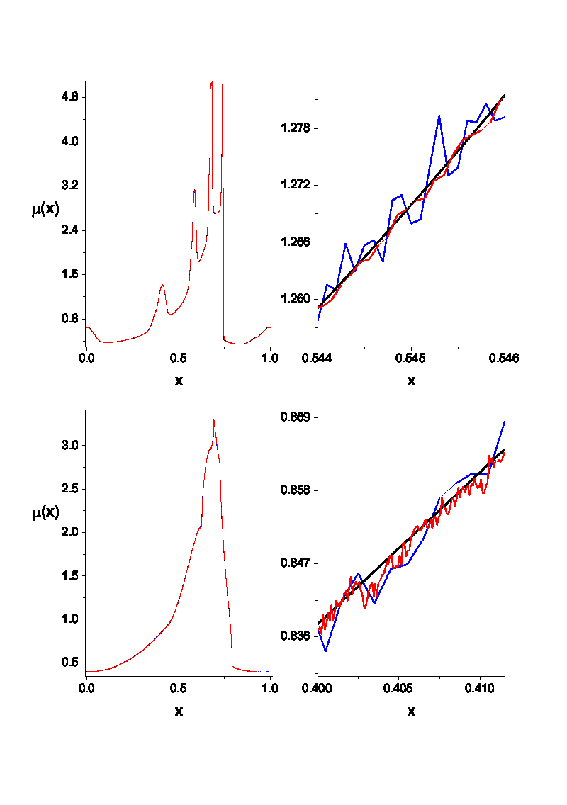
Figure 5. Comparison of the invariant measures computed using Ulam’s Monte Carlo algorithm (blue line) with the simulations of long orbits (red line) and the certified Ulam method (black line). Results plotted for $\epsilon=1.4$ and $\tau=0.709$. Top panels – noise amplitude $\xi=0.01$; and bottom panels – $\xi=0.1$. Note that in the left panels the three curves appear to coincide. The right panels show a zoom, in which smaller-scale differences between the three curves are visible.

6.4. Noise dependence of the rotation number’s monotonicity

In this section, we show numerical results that — while not rigorous — suggest that, as remarked in Section 5, the non-monotonicity of the rotation number is a phenomenon typical of small noise amplitudes that disappears as the noise amplitude is large enough. We consider the behavior of the rotation number in the interval of $\tau$ values $[0.707,0.716]$. We considered two amplitude of the noise: $\xi_{1}=0.01$ for which we known that the rotation number is non monotonic and $\xi_{2}=0.05$. The numerical simulations were carried out by using for each pair $(\tau,\epsilon)$, with $\epsilon=1.4$ and $\tau\in\left\{0.707,0.708,....,0.716\right\}$, 60000 independent noise realizations. Moreover, for each realization, the corresponding rotation number was estimated after $10^{6}$ iterates of the Arnold map. The corresponding results are reported in figure 6 and show that the rotation number becomes a monotonic function of $\tau$ when the noise amplitude is $\xi_{2}=0.05$.

We have seen that the presence of the noise promotes several effects on the dynamics of the corresponding noisy Arnold map. In particular, the results of the simulations discussed in Sections 6 and 6.4 leads to the following remarks:
a) The presence of noise determines an increase of the support of the corresponding invariant measure and to its smoothing.
b) The comparison of the measures computed with the three approaches shows good agreement among them; see left panels of figure 5. However, the inspection of these data on a finer scale, shows that the measures obtained with the Monte Carlo approaches exhibit fluctuations with respect to that computed with the certified method.
c) The noise amplitude strongly impacts the monotonicity properties of the rotation number: i.e., for sufficiently high noise amplitude, a transition from non-monotonic to monotonic behavior is observed.

To complete the above discussion, in figure 7 are reported the values of the rotation number against $\tau$ ($\epsilon=1.4$) in the case of zero noise and for a larger interval of $\tau$ values. These data were obtained using a Monte Carlo approach in which, for each $\tau$ value, the mean and standard deviation of $\rho_{\tau}$ were obtained by averaging over $10^{3}$ initial conditions (for each initial condition the corresponding rotation number was estimated after $10^{6}$ iteration of the noiseless map). The data clearly show the non monotonic behavior of the rotation number in the chosen interval of $\tau$ values. The data on the right of the figure also show that non monotonic behavior also occurs in other intervals of $\tau$ values (of smaller amplitude). For each $\tau$ the distribution of the corresponding $\rho_{\tau}$ values determined with this approach follow approximately a Gaussian distribution (data not shown). Then, using the standard t-test, it was found that the mean probability that the rotation number is monotonic in the intervals of interest is much lower than $10^{-3}$.

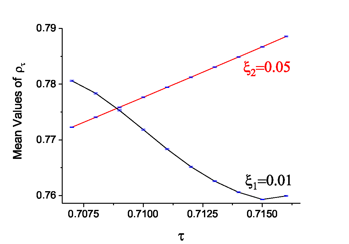
Figure 6. Effect of the noise amplitude on the monotonicity of the rotation number $\rho=\rho_{\tau}$, shown for $\epsilon=1.4$. The black line represents the numerical results for $\xi=0.01$, while the red line is for $\xi=0.05$. The errors bars represent the corresponding standard deviations.

Figure 7. Non monotonicity of the rotation number $\rho_{\tau}$ for $\epsilon=1.4$ and in absence of noise ($\xi=0$). The black dots represent the mean values of $\rho_{\tau}$, while the errorbars represent the corresponding standard deviations.

7. Concluding remarks

In this paper, we have studied Arnold circle maps with strong nonlinearity and additive noise. We have proven rigorously that the rotation number $\rho_{\tau}$ is differentiable with respect to the parameter $\tau$, whenever the stochastically perturbed map is mixing, providing a formula for the derivative of $\rho_{\tau}$ with respect to $\tau$. Moreover, we have shown, using a computer-aided proof, that $\rho_{\tau}$ is not necessarily monotonic for $\epsilon\geq 1.$

As outlined in the introduction, an important area of application of such maps is the study of the El Niño–Southern Oscillation (ENSO) phenomenon, which greatly affects seasonal-to-interannual climate variability. The computational tools used in this paper are not directly applicable to high-end, high-resolution global climate models (GCMs). But there are three ways in which the results of this paper may shed light on the behavior of such models and of the climate system itself.

First, the climate sciences have long relied on a systematic use of a hierarchy of models, from the simplest ones, such as Arnold circle maps [33] — through intermediate ones, such as those used to obtain Fig. 2 [45, 46] — and on to the most detailed GCMs [31, 36, 41, 66]. By applying systematically advanced statistical methods [32] to the simulations produced by models of increasing detail and resolution, on the one hand, and to observational data sets, on the other, it is possible to infer properties of models at the top of the hierarchy and of the climate system itself, given dynamical insights obtained with simple and intermediate models [31, 36].

Second, linear response theory has played a crucial role in the arguments developed in the present paper. This theory has already been applied fairly widely in the climate sciences ([52],[34],[40]). Linear response theory was proved to apply generally in random systems in which the presence of noise plays has a regulatizing effect ([40],[27]). We can expect, therefore, that several of the general ideas presented herein can be applied not only to very highly idealized models, like the Arnold circle map, but to intermediate climate models as well, in the presence of additive noise.

Third, methods of data-driven model building have been used to derive relatively simple models directly from observational data sets and from simulations of high-end models [43, 47, 49, 60]. With the greatly increased recent interest in such models in the era of big data, this avenue will permit the formulation of more sophisticated data-driven models that will be amenable to study by the full set methods described and used herein.

8. Acknowledgments

The rigorous computations presented in subsections 4.2 and 5 were performed on the supercomputer facilities of the Mésocentre de calcul de Franche-Comté.
JS was supported by the European Research Council (ERC) under the European Union’s Horizon 2020 research and innovation program (grant agreement No. 787304).

The present paper is TiPES contribution #4; this project has received funding from the European Union’s Horizon 2020 research and innovation program under grant agreement No. 820970.

References

- [1] Antown F, Dragičević.D, Froyland, G.: Optimal linear responses for Markov chains and stochastically perturbed dynamical systems. J. Stat Phys 170, 6, pp 1051–1087 (2018)
- [2] Arnold, V.I.: Small denominators. I: Mappings of the circumference onto itself. AMS Translations, Ser. 2 46, 213–284 (1965)
- [3] Arnold V.I.: Cardiac arrhythmias and circle mappings. Chaos: An Interdisciplinary J. Nonlin. Sci. 1, 20–24 (1991),
- [4] Arnold, V.I.: Geometrical Methods in the Theory of Differential Equations. Springer, 334 pp. (1983)
- [5] Bahsoun, W., Saussol, B.: Linear response in the intermittent family: differentiation in a weighted -norm. Discrete Contin. Dyn. Syst. 36(12), 6657-6668 (2016)
- [6] Bahsoun, W., Ruziboev, M., Saussol, B.: Linear response for random dynamical systems. arXiv:1710.03706
- [7] Bahsoun, W., Galatolo, S., Nisoli, I., Niu, X.: A Rigorous Computational Approach to Linear Response. Nonlinearity 31(no.3), 1073–1109 (2018)
- [8] Bailey, M.P., Drks, G.,Sheldonm A.C.: Circle maps with gaps: Understanding the dynamics of the two-process model for sleep–wake regulation. European Journal of Applied Mathematics, https://doi.org/10.1017/S0956792518000190 (2018),1-24.
- [9] Bak, P.: The devil’s staircase. Physics Today 39(12), 38–45 (1986)
- [10] Bak, P., and Bruinsma, R.: One-dimensional Ising model and the complete devil’s staircase. Phys. Rev. Lett. 49, 249-251 (1982)
- [11] Baladi, V.: On the susceptibility function of piecewise expanding interval maps. Comm. Math. Phys. 275(3), 839-859 (2007)
- [12] Baladi, V., Todd, M.: Linear response for intermittent maps. Comm. Math. Phys. 347(3), 857-874 (2016)
- [13] Baladi, V., Smania, D.: Linear response formula for piecewise expanding unimodal maps. Nonlinearity 21(4), 677-711 (2008)
- [14] Baladi, V.: Linear response, or else Proceedings of the International Congress of Mathematicians—Seoul 2014. Vol. III, 525–545 (2014)
- [15] Baladi, V., Benedicks, M., Schnellmann, N.: Whitney-Holder continuity of the SRB measure for transversal families of smooth unimodal maps. Invent. Math. 201, 773-844 (2015)
- [16] Baladi, V., Kuna, T., Lucarini, V.: Linear and fractional response for the SRB measure of smooth hyperbolic attractors and discontinuous observables. Nonlinearity 30, 1204-1220 (2017)
- [17] Barnston, A.G., Tippett, M.K., L’Heureux, M., Li, S., DeWitt, D.G.: Skill of real-time seasonal ENSO model predictions during 2002–11: Is our capability increasing?. Bull. Am. Meteorol. Soc., 93(5), 631–651 (2012).
- [18] Batista, A.M., Sandro, E., Pinto, de S., Viana, R.L.,Lopes, S.R.: Mode locking in small-world networks of coupled circle maps. Physica A: Statistical Mechanics and its Applications 322, 118-128 (2003)
- [19] Bose, C. J., Murray R.: The exact rate of approximation in Ulam’s method. Discrete and Continuous Dynamical Systems 7, 219-235 (2001)
- [20] Chang, P., Wang, B., Li, T., Ji, L.: Interactions between the seasonal cycle and the Southern Oscillation: Frequency entrainment and chaos in intermediate coupled ocean-atmosphere model. Geophys. Res. Lett. 21, 2817–2820 (1994)
- [21] Chang, P., Ji, L., Li, T., Flügel, M.: Chaotic dynamics versus stochastic processes in El Niño-Southern Oscillation in coupled ocean-atmosphere models. Physica D 98, 301–320 (1996)
- [22] Chekroun, , M.D., Simonnet, E., Ghil M.: Stochastic climate dynamics: Random attractors and time-dependent invariant measures. Physica D 240(21), 1685–1700, (2011)
- [23] Dolgopyat, D.: On differentiability of SRB states for partially hyperbolic systems. Invent. Math. 155(2), 389-449 (2004)
- [24] Ding, J., Wang, Z.: Parallel Computation of invariant measures. Annals of Operations Research 103, 283-290 (2001)
- [25] Eisenman, I., Yu, L., Tziperman, E.: Westerly wind bursts: ENSO tail rather than the dog?. J. Climate 18, 5224–5238 (2005)
- [26] Feigenbaum, M.J., Kadanoff, L.P., Shenker, S.J.: Quasiperiodicity in dissipative systems: A renormalization group analysis. Physica D 5, 370–386 (1982)
- [27] Galatolo, S., Giulietti, P.: Linear response for dynamical systems with additive noise. Nonlinearity 32, n. 6 pp. 2269-2301 (2019)
- [28] Galatolo, S.: Quantitative statistical stability and speed of convergence to equilibrium for partially hyperbolic skew products.J. Éc. Polytech. Math. 5, 377–405 (2018)
- [29] Galatolo, S., Monge, M., Nisoli, I.: Existence of noise induced order, a computer aided proof. arXiv:1702.07024
- [30] Galatolo, S., Pollicott, M.: Controlling the statistical properties of expanding maps. Nonlinearity 30, 2737-2751 (2017)
- [31] Ghil, M.: Hilbert problems for the geosciences in the 21st century. Nonlin. Processes Geophys. 8, 211–222 (2001)
- [32] Ghil, M., Allen, M.R., Dettinger, M.D., Ide, K., Kondrashov, D., Mann, M.E., Robertson, A.W., Saunders, A., Tian, Y., Varadi, F., Yiou, P.: Advanced spectral methods for climatic time series. Rev. Geophys. 40(1), doi:10.1029/2000RG000092 (2002)
- [33] M. Ghil, M., Chekroun, M.D., Simonnet, E.: Climate dynamics and fluid mechanics: Natural variability and related uncertainties. Physica D 237, 2111–2126, doi:10.1016/j.physd.2008.03.036 (2008)
- [34] Ghil, M. and V. Lucarini The physics of climate variability and climate change Rev. Mod. Phys., submitted, arXiv:1910.00583
- [35] Ghil, M., Jiang, N.: Recent forecast skill for the El Niño/Southern Oscillation. Geophys. Res. Lett. 25, 171–174 (1998)
- [36] Ghil, M., Robertson, A.W.: Solving problems with GCMs: General circulation models and their role in the climate modeling hierarchy.In D. Randall (Ed.) General Circulation Model Development: Past, Present and Future, Academic Press, San Diego, 285–325 (2000)
- [37] Ghil, M., Zaliapin I., Thompson, S.: A delay differential model of ENSO variability: Parametric instability and the distribution of extremes. Nonlin. Processes Geophys. 15, 417–433 (2008)
- [38] Ghil, M. The wind-driven ocean circulation: Applying dynamical systems theory to a climate problem, Discr. Cont. Dyn. Syst. – A, 37(1), 189–228 (2017)
- [39] Glass L.: Cardiac arrhythmias and circle maps- A classical problem. Chaos: An Interdisciplinary Journal of Nonlinear Science 1, 13–19 (1991)
- [40] Hairer, M., Majda, A.J.: A simple framework to justify linear response theory. Nonlinearity 23, 909–922 (2010)
- [41] Held, I.M.: The gap between simulation and understanding in climate modeling. Bull. Am. Meteorol. Soc. 86, 1609–1614 (2005)
- [42] Keener, J.P., Glass, L.: Global bifurcations of a periodically forced nonlinear oscillator. J. Math. Biology 21, 175–190 (1984)
- [43] Kondrashov, D., Chekroun, M.D., Yuan, X., Ghil, M.: Data-adaptive harmonic decomposition and stochastic modeling of Arctic sea ice. in Nonlinear Advances in Geosciences, A. Tsonis, Ed., Springer Science & Business Media, 179–206, doi:10.1007/978-3-319-58895-7 (2018)
- [44] Jiang, S., F.-F. Jin, and M. Ghil, Multiple equilibria, periodic, and aperiodic solutions in a wind-driven, double-gyre, shallow-water model, J. Phys. Oceanogr., 25, 764–786. (1995)
- [45] Jin, F.-F., Neelin J.D., Ghil, M.: El Niño on the Devil’s Staircase: Annual subharmonic steps to chaos. Science 264, 70–72 (1994)
- [46] Jin, F.-F., Neelin J.D., Ghil, M.: El Niño/Southern Oscillation and the annual cycle: Subharmonic frequency locking and aperiodicity. Physica D 98, 442–465 (1996)
- [47] Kondrashov, D., Chekroun M.D., Ghil, M.: Data-driven non-Markovian closure models. Physica D 297, 33–55, doi:10.1016/j.physd.2014.12.005 (2015)
- [48] Korepanov, A.: Linear response for intermittent maps with summable and nonsummable decay of correlations. Nonlinearity 29(6), pp. 1735-1754 (2016)
- [49] Kravtsov, S., Kondrashov, D., Ghil, M.: Empirical model reduction and the modelling hierarchy in climate dynamics and the geosciences. in Stochastic Physics and Climate Modelling, T. Palmer and P. Williams (Eds.), Cambridge Univ. Press, pp. 35–72 (2009)
- [50] Lasota, A., Mackey, M.C.: Probabilistic Properties of Deterministic Systems. Cambridge University Press (1986)
- [51] Liverani, C.: Invariant measures and their properties: A functional analytic point of view. Dynamical systems. Part II, pp. 185-237, Pubbl. Cent. Ric. Mat. Ennio Giorgi, Scuola Norm. Sup., Pisa (2003)
- [52] Lucarini, V.: Stochastic perturbations to dynamical systems: A response theory approach. J. Stat. Phys. 146(4), 774–786 (2012)
- [53] Latif, M., Barnett, T.P., Flügel, M., Graham, N.E., Xu, J-S., Zebiak, S.E.: A review of ENSO prediction studies. Clim. Dyn. 9, 167–179 (1994)
- [54] Lorenz, E. N., Deterministic nonperiodic flow. J. Atmos. Sci., 20, 130–141. (1963)
- [55] Lorenz, E. N., The mechanics of vacillation. J. Atmos. Sci., 20, 448–464. (1963)
- [56] MacKay, R.S.: Management of complex dynamical systems. Nonlinearity 31(n.2), 52-64 (2018)
- [57] Murray, R.: Optimal partition choice for invariant measure approximation for one-dimensional maps. Nonlinearity 17, 1623-1644 (2004)
- [58] Neelin, J.D., Battisti, D.S., Hirst, A.C., et al.: ENSO theory. J. Geophys. Res.–Oceans, 103(C7), 14261–14290 (1998)
- [59] Palmer, T., Williams, P., (Eds.): Stochastic Physics and Climate Modelling. Cambridge University Press, Cambridge, UK, (2009)
- [60] Penland, C.: A stochastic model of Indo-Pacific sea-surface temperature anomalies. Physica D 98, 534–558 (1996)
- [61] Pierini, S., M. Ghil and M. D. Chekroun, Exploring the pullback attractors of a low-order quasigeostrophic ocean model: The deterministic case, J. Climate, 29, 4185–4202 (2016) .
- [62] Philander, S.G.H.: El Niño, La Niña, and the Southern Oscillation. Academic Press, San Diego, (1990)
- [63] Pollicott, M., Vytnova, P.: Linear response and periodic points. Nonlinearity 29(no.10), 3047–3066 (2016)
- [64] Ruelle, D.: Differentiation of SRB states. Commun. Math. Phys. 187, pp. 227-241 (1997)
- [65] Saunders A., Ghil, M.: A Boolean delay equation model of ENSO variability. Physica D 160, 54–78 (2001)
- [66] Schneider, S.H., Dickinson, R.E.: Climate modeling. Rev. Geophys. Space Phys. 12, 447–493 (1974)
- [67] Sedro, J.: A regularity result for fixed points, with applications to linear response. arXiv:1705.04078
- [68] Timmermann, A., Jin, F-F.: A nonlinear mechanism for decadal El Niño amplitude changes. Geophys. Res. Lett. 29(1), https://doi.org/10.1029/2001GL013369 (2002)
- [69] Tziperman, E., Stone, L., Cane, M., Jarosh, H.: El Niño chaos: Overlapping of resonances between the seasonal cycle and the Pacific ocean-atmosphere oscillator. Science 264, 72–74 (1994)
- [70] Tziperman, E., Cane, M.A., Zebiak, S.E.: Irregularity and locking to the seasonal cycle in an ENSO prediction model as explained by the quasi-periodicity route to chaos. J. Atmos. Sci. 50, 293–306 (1995)
- [71] Tucker, W.: Validated Numerics A Short Introduction to Rigorous Computations. Princeton Univ. Press (2011)
- [72] Ulam, S.M.:: A Collection of Mathematical Problems. Interscience Publisher NY, 1960
- [73] Verbickas, S.: Westerly wind bursts in the tropical Pacific. Weather 53, 282–284 (1998)
- [74] Viana, M.: Lectures on Lyapunov Exponents. Cambridge Studies in Advanced Mathematics 145, Cambridge University Press (2014)
- [75] Wiggins, S.: Introduction to Applied Dynamical Systems and Chaos. Springer NY, (2003) (see theorem 21.6.16)
- [76] Zaliapin, I., Ghil, M.: A delay differential model of ENSO variability, Part 2: Phase locking, multiple solutions and dynamics of extrema. Nonlin. Processes Geophys. 17, 123–135 (2010)
- [77] Zhang, Z.: On the smooth dependence of SRB measures for partially hyperbolic systems. arXiv:1701.05253
- [78] Zmarrou, H., Homburg., A.J.: Bifurcations of stationary measures of random diffeomorphisms. Ergodic Theory Dynam. Systems 27(5):1651–1692 (2007)
- [79] Herman, M.R.: Mesure de Lebesgue et nombre de rotation, in: Geometry and Topology (Proc. III Latin Amer. School of Math., Inst. Mat. Pura Aplicada CNPq, Rio de Janeiro, 1976). Lecture Notes in Math., vol.597, Springer, Berlin, pp. 271–-293 (1977)
- [80] Katok, A., Hasselblatt, B.: Introduction to the modern theory of dynamical systems. Cambridge University Press, (1995)
- [81] Matsumoto, S.: Derivatives of the rotation number of one parameter families of circle diffeomorphisms. Kodai Mat. J. 35:115–125 (2012)
- [82] Luque, A., Villanueva, J.: Computation of the derivatives of the rotation number for parametric families of circle diffeomorphisms. Physica D 237:2599–2615 (2008)