General Risk Measures
for Robust Machine Learning

Abstract

A wide array of machine learning problems are formulated as the minimization of the expectation of a convex loss function on some parameter space. Since the probability distribution of the data of interest is usually unknown, it is is often estimated from training sets, which may lead to poor out-of-sample performance. In this work, we bring new insights in this problem by using the framework which has been developed in quantitative finance for risk measures. We show that the original min-max problem can be recast as a convex minimization problem under suitable assumptions. We discuss several important examples of robust formulations, in particular by defining ambiguity sets based on $\varphi$-divergences and the Wasserstein metric. We also propose an efficient algorithm for solving the corresponding convex optimization problems involving complex convex constraints. Through simulation examples, we demonstrate that this algorithm scales well on real data sets.

Keywords: Risk measures, robust statistics, machine learning, convex optimization, divergences, Wasserstein distance.

1 Introduction

In machine learning, the robustness of the solutions obtained for classification and prediction tasks remains a main issue. In Papernot, McDaniel, and Goodfellow (2016) and Kurakin, Goodfellow, and Bengio (2016), some examples are provided where small modifications of the input data can completely alter the resulting solution. In Feng, Xu, Mannor, and Yan (2014) and Plan and Vershynin (2013), poor out-of-sample performances are displayed when training data is sparse. This kind of problems also occurs in optimal control when there exist uncertainties on parameters. In Ben-Tal and Nemirovski (2000), the authors showed that a small perturbation on the parameters can turn a feasible solution into an infeasible one.

In this context, robust approaches appear as a way of controlling out-of-sample performance. There is an extensive literature dealing with robust problems and the reader is refered to Ben-Tal, El Ghaoui, and Nemirovski (2009) for a survey. One of the main approaches consists of introducing constraints on the probability distribution of the unknown data. Under some conditions, this approach is equivalent to deal with ambiguity sets or a modified loss function. The works in Ben-Tal, Den Hertog, De Waegenaere, Melenberg, and Rennen (2013); Hu and Hong (2013); Duchi, Glynn, and Namkoong (2016); Moghaddam and Mahlooji (2016) and Namkoong and Duchi (2016) have brought more insight on ambiguity sets. In Esfahani and Kuhn (2015) and Esfahani, Shafieezadeh-Abadeh, Hanasusanto, and Kuhn (2017), the authors present a distributionally robust optimization framework based on the Wasserstein distance. A set of probability distributions is defined as a ball centered on the reference probability with respect to the Wasserstein distance, then the optimization is carried out for the worst cost over this probability set.

This idea of minimizing the worst cost over a given probability set is well-known in quantitative finance. The robust representation of risk measures provides a theoretical framework to do so. A rich class of risk measures is the class of coherent ones which were introduced in the seminal paper by Artzner, Delbaen, Eber, and Heath (1999). In Föllmer and Schied (2016), a broader class of so-called convex risk measures was investigated, for which a large number of results were established.

In this paper, we follow the line of Esfahani and Kuhn (2015), which aims at reformulating robust problems using ambiguity sets as convex minimization problems. Our contribution is threefold. First we clarify the links existing between risk measures and robust optimization. This allows us to transpose results from finance to machine learning. Second, we propose a unifying convex optimization setting for dealing with various risk measures, including those based on $\varphi$-divergences or the Wasserstein distance. Finally, we propose an accelerated algorithm grounded on the subgradient projection method proposed in Combettes (2003). We show that the proposed algorithm is able to solve efficiently large-scale robust problems.

The organization of the paper is as follows. In Section 2, we state the general mathematical problem we investigate in the context of machine learning. In Section 3, we first draw a parallel between this problem and convex monetary risk measures. We then provide a convex reformulation of the problem. In Section 4, we discuss some important classes of risk measures by revisiting some of the results in the literature. In Section 5, we describe our algorithm for solving convex formulations of robust problems. Then, in Section 6, we illustrate the good performance of the proposed algorithm through numerical experiments on real datasets. Finally, short concluding remarks are made in Section 7.

2 Problem statement

Let $(\Omega,\mathscr{F},p)$ be the underlying probability space where $\Omega$ is a finite set of cardinal $N$, $\mathscr{F}$ is the $\sigma$-field generated by $(\{\omega\})_{\omega\in\Omega}$, and $p$ is a probability distribution that is assumed to charge all points. Let $d$ be a nonzero integer and let $\mathbf{z}\colon\Omega\to\mathbb{R}^{d}$ denote a general random variable. Note that function $\mathbf{z}$ can be identified with a matrix in $\mathbb{R}^{N\times d}$ where, for every $i\in[\![1,N]\!]$, $z_{i}\in\mathbb{R}^{d}$ is the vector corresponding to the $i$-th line of matrix $\mathbf{z}$ . We denote by $\mathcal{M}_{1}$ the set of probability distributions over $(\Omega,\mathscr{F},p)$.

For every $i\in[\![1,N]\!]$, let $\ell(\cdot,z_{i})\colon\mathbb{R}^{n}\to\mathbb{R}\cup\{+\infty\}$ be a loss function which is assumed to be lower semicontinuous (lsc) and convex such that

$$\bigcap_{i=1}^{N}\mathop{\mathrm{dom}}\big{(}\ell(\cdot,z_{i})\big{)}\neq\varnothing\;,$$ (1)

where $\mathop{\mathrm{dom}}(g)$ denotes the domain of a function $g$, that is the set of argument values for which this function is finite. In standard formulations of machine learning problems, one aims at finding an optimal regression vector $\overline{\theta}\in\mathbb{R}^{n}$ such that

$$\overline{\theta}\in\mathop{\arg\min}_{\theta\in\mathbb{R}^{n}}\sum_{i=1}^{N}p_{i}\ell(\theta,z_{i})\;.$$ (2)

Indeed, setting $z_{i}=[x_{i}^{\top}\;\;y_{i}]^{\top}$ with $n=d-1\geq 1$, $x_{i}\in\mathbb{R}^{n}$, and $y_{i}\in\mathbb{R}$ allows us to recover a wide array of estimation and classification problems. For example, penalized least squares regression problems are obtained when

$$(\forall i\in[\![1,N]\!])(\forall\theta\in\mathbb{R}^{n})\quad\ell(\theta,z_{i})=\frac{1}{2}\|y_{i}-x_{i}^{\top}\theta\|^{2}+\rho(\theta)\;,$$ (3)

where $\rho\colon\mathbb{R}^{n}\to\mathbb{R}\cup\{+\infty\}$ is a proper, lsc, convex penalty function. If the random variable $\mathbf{y}$ is $\{0,1\}$-valued, we can recover binary classification problems, for example by performing a logistic regression, i.e.

$$(\forall i\in[\![1,N]\!])(\forall\theta\in\mathbb{R}^{n})\quad\ell(\theta,z_{i})=\log\Big{(}1+\exp\big{(}-y_{i}x_{i}^{\top}\theta\big{)}\Big{)}\;.$$ (4)

One of the main limitations of this formulation is that it assumes that the true probability distribution of the data is perfectly known. In practice, this distribution is often estimated empirically from the available observations.

In this paper, we will focus on the following more general robust formulation to determine an optimal regression vector.

Problem 1.

Let $\alpha\colon\mathbb{R}^{N}\to\mathbb{R}\cup\{+\infty\}$ be a lsc convex penalty function whose domain is a nonempty subset of $\mathcal{M}_{1}$. We want to find

$$\overline{\theta}\in\mathop{\arg\min}_{\theta\in\mathbb{R}^{n}}\sup_{q=(q_{i})_{1\leq i\leq N}\in\mathcal{M}_{1}}\left(\sum_{i=1}^{N}q_{i}\ell(\theta,z_{i})-\alpha(q)\right)\;,$$ (5)

In this problem, if $\alpha$ is the indicator function $\iota_{\{p\}}$ of the singleton containing a probability distribution $p$, then (2) is recovered. More generally, if $\alpha$ is equal to the indicator function of a nonempty closed convex set $\mathcal{Q}\subset\mathcal{M}_{1}$, then the objective function in (5) reduces to

$$\sup_{q\in\mathcal{Q}}\sum_{i=1}^{N}q_{i}\ell(\theta,z_{i})=\sigma_{\mathcal{Q}}\big{(}\mathbf{\ell}(\theta,\mathbf{z})\big{)}\;,$$ (6)

where $\sigma_{\mathcal{Q}}$ is the support function of $\mathcal{Q}$. This corresponds to the well-known case of distributionally robust optimization using ambiguity sets Esfahani and Kuhn (2015).

3 Convex formulation of robust inference problems using risk measures

In this section, we address Problem 1 in the light of the financial framework for monetary risk measures. We first recall known properties of risk measures and then show how Problem 1 can be reformulated as a convex problem.

3.1 Definition and properties of a risk measure

Let $\mathbb{X}$ be the space of real-valued random variables defined on the probability space $(\Omega,\mathscr{F},p)$. We denote by $\boldsymbol{X^{\textstyle\text{\unboldmath$\scriptstyle$}}_{\textstyle\text{\unboldmath$\scriptstyle$}}}$ a generic element of $\mathbb{X}$ and we recall that $p$ is assumed to be a distribution that charges all points. The space $\mathbb{X}$ is endowed with the pointwise order $\leq$, that is,

$$(\forall(\boldsymbol{X^{\textstyle\text{\unboldmath$\scriptstyle$}}_{\textstyle\text{\unboldmath$\scriptstyle$}}},\boldsymbol{Y^{\textstyle\text{\unboldmath$\scriptstyle$}}_{\textstyle\text{\unboldmath$\scriptstyle$}}})\in\mathbb{X}^{2})\quad\boldsymbol{X^{\textstyle\text{\unboldmath$\scriptstyle$}}_{\textstyle\text{\unboldmath$\scriptstyle$}}}\leq\boldsymbol{Y^{\textstyle\text{\unboldmath$\scriptstyle$}}_{\textstyle\text{\unboldmath$\scriptstyle$}}}\Leftrightarrow(\forall\omega\in\Omega)\;\;\boldsymbol{X^{\textstyle\text{\unboldmath$\scriptstyle$}}_{\textstyle\text{\unboldmath$\scriptstyle$}}}(\omega)\leq\boldsymbol{Y^{\textstyle\text{\unboldmath$\scriptstyle$}}_{\textstyle\text{\unboldmath$\scriptstyle$}}}(\omega)\;.$$ (7)

A risk measure $\mathbb{F}$ is a real-valued function $\mathbb{F}:\mathbb{X}\to\mathbb{R}\;.$
The next four properties of risk measures were first introduced in Artzner, Delbaen, Eber, and Heath (1999) to define the so called coherent risk measures. The interested reader can also refer to Föllmer and Schied (2016)[Part I, Chapter 4].

Definition 1.

A risk measure $\mathbb{F}\colon\mathbb{X}\to\mathbb{R}$ is said to be

• monotone: if, for every $(\boldsymbol{X^{\textstyle\text{\unboldmath$\scriptstyle$}}_{\textstyle\text{\unboldmath$\scriptstyle$}}},\boldsymbol{Y^{\textstyle\text{\unboldmath$\scriptstyle$}}_{\textstyle\text{\unboldmath$\scriptstyle$}}})\in\mathbb{X}^{2}$, $\boldsymbol{X^{\textstyle\text{\unboldmath$\scriptstyle$}}_{\textstyle\text{\unboldmath$\scriptstyle$}}}\leq\boldsymbol{Y^{\textstyle\text{\unboldmath$\scriptstyle$}}_{\textstyle\text{\unboldmath$\scriptstyle$}}}\Rightarrow\mathbb{F}[\boldsymbol{X^{\textstyle\text{\unboldmath$\scriptstyle$}}_{\textstyle\text{\unboldmath$\scriptstyle$}}}]\leq\mathbb{F}[\boldsymbol{Y^{\textstyle\text{\unboldmath$\scriptstyle$}}_{\textstyle\text{\unboldmath$\scriptstyle$}}}]$,

• translation invariant: if, for every $\boldsymbol{X^{\textstyle\text{\unboldmath$\scriptstyle$}}_{\textstyle\text{\unboldmath$\scriptstyle$}}}\in\mathbb{X}$ and $m\in\mathbb{R}$, $\mathbb{F}[\boldsymbol{X^{\textstyle\text{\unboldmath$\scriptstyle$}}_{\textstyle\text{\unboldmath$\scriptstyle$}}}+m]=\mathbb{F}[\boldsymbol{X^{\textstyle\text{\unboldmath$\scriptstyle$}}_{\textstyle\text{\unboldmath$\scriptstyle$}}}]+m$,

• convex: if, for every $(\boldsymbol{X^{\textstyle\text{\unboldmath$\scriptstyle$}}_{\textstyle\text{\unboldmath$\scriptstyle$}}},\boldsymbol{Y^{\textstyle\text{\unboldmath$\scriptstyle$}}_{\textstyle\text{\unboldmath$\scriptstyle$}}})\in\mathbb{X}^{2}$ and $\lambda\in]0,1[$, $\mathbb{F}\big{[}\lambda\boldsymbol{X^{\textstyle\text{\unboldmath$\scriptstyle$}}_{\textstyle\text{\unboldmath$\scriptstyle$}}}+(1-\lambda)\boldsymbol{Y^{\textstyle\text{\unboldmath$\scriptstyle$}}_{\textstyle\text{\unboldmath$\scriptstyle$}}}\big{]}\leq\lambda\mathbb{F}[\boldsymbol{X^{\textstyle\text{\unboldmath$\scriptstyle$}}_{\textstyle\text{\unboldmath$\scriptstyle$}}}]+(1-\lambda)\mathbb{F}[\boldsymbol{Y^{\textstyle\text{\unboldmath$\scriptstyle$}}_{\textstyle\text{\unboldmath$\scriptstyle$}}}]$,

• positively homogeneous: if, for every $\boldsymbol{X^{\textstyle\text{\unboldmath$\scriptstyle$}}_{\textstyle\text{\unboldmath$\scriptstyle$}}}\in\mathbb{X}$ and $\lambda\in[0,+\infty[$, $\mathbb{F}[\lambda\boldsymbol{X^{\textstyle\text{\unboldmath$\scriptstyle$}}_{\textstyle\text{\unboldmath$\scriptstyle$}}}]=\lambda\mathbb{F}[\boldsymbol{X^{\textstyle\text{\unboldmath$\scriptstyle$}}_{\textstyle\text{\unboldmath$\scriptstyle$}}}]$.

A risk measure which satisfies the first two properties is called a monetary risk measure. A risk measure which satisfies the first three properties is called a convex risk measure. A risk measure which satisfies the four properties is called a coherent risk measure.

Depending on the author, the first axiom may also be expressed as: for every $(\boldsymbol{X^{\textstyle\text{\unboldmath$\scriptstyle$}}_{\textstyle\text{\unboldmath$\scriptstyle$}}},\boldsymbol{Y^{\textstyle\text{\unboldmath$\scriptstyle$}}_{\textstyle\text{\unboldmath$\scriptstyle$}}})\in\mathbb{X}^{2}$, $\boldsymbol{X^{\textstyle\text{\unboldmath$\scriptstyle$}}_{\textstyle\text{\unboldmath$\scriptstyle$}}}\leq\boldsymbol{Y^{\textstyle\text{\unboldmath$\scriptstyle$}}_{\textstyle\text{\unboldmath$\scriptstyle$}}}\Rightarrow\mathbb{F}[\boldsymbol{X^{\textstyle\text{\unboldmath$\scriptstyle$}}_{\textstyle\text{\unboldmath$\scriptstyle$}}}]\geq\mathbb{F}[\boldsymbol{Y^{\textstyle\text{\unboldmath$\scriptstyle$}}_{\textstyle\text{\unboldmath$\scriptstyle$}}}]$ if the variables $\boldsymbol{X^{\textstyle\text{\unboldmath$\scriptstyle$}}_{\textstyle\text{\unboldmath$\scriptstyle$}}}$ and $\boldsymbol{Y^{\textstyle\text{\unboldmath$\scriptstyle$}}_{\textstyle\text{\unboldmath$\scriptstyle$}}}$ are interpreted as gains instead of a losses, which is a common in finance. For this reason, some sign differences may appear between results of various authors. We have chosen to follow the paths in Rockafellar and Uryasev (2000); Ruszczynski and Shapiro (2006); Ruszczyński and Shapiro (2006) and interpret the random variable in argument as a loss. We however often refer to Föllmer and Schied (2016), providing a comprehensive view of risk measures, where the opposite convention has been adopted.

Remark 2.

1. It readily follows from the translation invariance property that a monetary risk measure $\mathbb{F}$ admits a primal form given by

   $$(\forall\boldsymbol{X^{\textstyle\text{\unboldmath$\scriptstyle$}}_{\textstyle\text{\unboldmath$\scriptstyle$}}}\in\mathbb{X})\quad\mathbb{F}[\boldsymbol{X^{\textstyle\text{\unboldmath$\scriptstyle$}}_{\textstyle\text{\unboldmath$\scriptstyle$}}}]=\inf_{s\in\mathbb{R}}\{s\mid\boldsymbol{X^{\textstyle\text{\unboldmath$\scriptstyle$}}_{\textstyle\text{\unboldmath$\scriptstyle$}}}-s\in\operatorname{lev}_{\leq 0}\mathbb{F}\}\;,$$ (8)

   where $\operatorname{lev}_{\leq 0}\mathbb{F}$ is the lower level set of $\mathbb{F}$ at height 0 defined as

   $$\operatorname{lev}_{\leq 0}\mathbb{F}=\big{\{}\boldsymbol{X^{\textstyle\text{\unboldmath$\scriptstyle$}}_{\textstyle\text{\unboldmath$\scriptstyle$}}}\in\mathbb{X}\mid\mathbb{F}\big{[}\boldsymbol{X^{\textstyle\text{\unboldmath$\scriptstyle$}}_{\textstyle\text{\unboldmath$\scriptstyle$}}}\big{]}\leq 0\big{\}}\;.$$ (9)

2. A monetary risk measure $\mathbb{F}$ is $1$-Lipschitz continuous with respect to the supremum norm $\|\cdot\|_{\infty}$. Indeed, for every $(\boldsymbol{X^{\textstyle\text{\unboldmath$\scriptstyle$}}_{\textstyle\text{\unboldmath$\scriptstyle$}}},\boldsymbol{Y^{\textstyle\text{\unboldmath$\scriptstyle$}}_{\textstyle\text{\unboldmath$\scriptstyle$}}})\in\mathbb{X}^{2}$, we have $\boldsymbol{X^{\textstyle\text{\unboldmath$\scriptstyle$}}_{\textstyle\text{\unboldmath$\scriptstyle$}}}\leq\boldsymbol{Y^{\textstyle\text{\unboldmath$\scriptstyle$}}_{\textstyle\text{\unboldmath$\scriptstyle$}}}+\|\boldsymbol{X^{\textstyle\text{\unboldmath$\scriptstyle$}}_{\textstyle\text{\unboldmath$\scriptstyle$}}}-\boldsymbol{Y^{\textstyle\text{\unboldmath$\scriptstyle$}}_{\textstyle\text{\unboldmath$\scriptstyle$}}}\|$. By monotonicity and translation invariance we obtain that $\mathbb{F}[\boldsymbol{X^{\textstyle\text{\unboldmath$\scriptstyle$}}_{\textstyle\text{\unboldmath$\scriptstyle$}}}]-\mathbb{F}[\boldsymbol{Y^{\textstyle\text{\unboldmath$\scriptstyle$}}_{\textstyle\text{\unboldmath$\scriptstyle$}}}]\leq\|\boldsymbol{X^{\textstyle\text{\unboldmath$\scriptstyle$}}_{\textstyle\text{\unboldmath$\scriptstyle$}}}-\boldsymbol{Y^{\textstyle\text{\unboldmath$\scriptstyle$}}_{\textstyle\text{\unboldmath$\scriptstyle$}}}\|_{\infty}$, which by symmetry implies that $|\mathbb{F}[\boldsymbol{X^{\textstyle\text{\unboldmath$\scriptstyle$}}_{\textstyle\text{\unboldmath$\scriptstyle$}}}]-\mathbb{F}[\boldsymbol{Y^{\textstyle\text{\unboldmath$\scriptstyle$}}_{\textstyle\text{\unboldmath$\scriptstyle$}}}]|\leq\|\boldsymbol{X^{\textstyle\text{\unboldmath$\scriptstyle$}}_{\textstyle\text{\unboldmath$\scriptstyle$}}}-\boldsymbol{Y^{\textstyle\text{\unboldmath$\scriptstyle$}}_{\textstyle\text{\unboldmath$\scriptstyle$}}}\|_{\infty}$.

The class of convex risk measures includes a large number of useful functions. Without entering into details, we should mention: expectation, worst case, quantile, median, and average value at risk Föllmer and Schied (2016).

3.2 Convex reformulation

In this section, we will show that the “min-max” problem 1 admits a convex reformulation. We first gather in the following proposition some existing results in the literature.

Proposition 3.

$\mathbb{F}{}$ is a convex risk measure if and only if there exists a lsc and convex function $\alpha\colon\mathbb{R}^{N}\to\mathbb{R}\cup\{+\infty\}$ such that

$$(\forall\boldsymbol{X^{\textstyle\text{\unboldmath$\scriptstyle$}}_{\textstyle\text{\unboldmath$\scriptstyle$}}}\in\mathbb{X})\quad\mathbb{F}[\boldsymbol{X^{\textstyle\text{\unboldmath$\scriptstyle$}}_{\textstyle\text{\unboldmath$\scriptstyle$}}}]=\sup_{q\in\mathcal{M}_{1}}\left(\sum_{i=1}^{N}q_{i}x_{i}-\alpha(q)\right)\;.$$ (10)

The function $\alpha$ associated with $\mathbb{F}{}$ is uniquely defined as

$$(\forall q\in\mathbb{R}^{N})\quad\alpha(q)=\begin{cases}\displaystyle\sup_{\boldsymbol{X^{\textstyle\text{\unboldmath$\scriptstyle$}}_{\textstyle\text{\unboldmath$\scriptstyle$}}}\in\operatorname{lev}_{\leq 0}\mathbb{F}}\mathbb{E}_{q}[\boldsymbol{X^{\textstyle\text{\unboldmath$\scriptstyle$}}_{\textstyle\text{\unboldmath$\scriptstyle$}}}]&\mbox{if $q\in\mathcal{M}_{1}\;,$}\\ +\infty&\mbox{otherwise}\;.\end{cases}$$ (11)

In addition, $\mathbb{F}{}$ is coherent if and only if its conjugate function $\alpha$ is the indicator function of a nonempty closed convex subset of $\mathcal{M}_{1}$.

Proof.

1. We know from Föllmer and Schied (2016, Theorem 4.16 and Proposition 4.15) that any convex risk measure $\mathbb{F}$ on $\mathbb{X}$ is of the form

   $$(\forall\boldsymbol{X^{\textstyle\text{\unboldmath$\scriptstyle$}}_{\textstyle\text{\unboldmath$\scriptstyle$}}}\in\mathbb{X})\quad\mathbb{F}[\boldsymbol{X^{\textstyle\text{\unboldmath$\scriptstyle$}}_{\textstyle\text{\unboldmath$\scriptstyle$}}}]=\sup_{q\in\mathcal{M}_{1}}\big{(}\mathbb{E}_{q}[\boldsymbol{X^{\textstyle\text{\unboldmath$\scriptstyle$}}_{\textstyle\text{\unboldmath$\scriptstyle$}}}]-\alpha(q)\big{)}\;,$$ (12)

   where $\alpha\colon\mathbb{R}^{N}\to\mathbb{R}\cup\{+\infty\}$ is the lsc and convex function whose domain is a nonempty subset of $\mathcal{M}_{1}$, given by

   $$(\forall q\in\mathcal{M}_{1})\quad\alpha(q) =\sup_{\boldsymbol{X^{\textstyle\text{\unboldmath$\scriptstyle$}}_{\textstyle\text{\unboldmath$\scriptstyle$}}}\in\mathbb{X}}\mathbb{E}_{q}[\boldsymbol{X^{\textstyle\text{\unboldmath$\scriptstyle$}}_{\textstyle\text{\unboldmath$\scriptstyle$}}}]-\mathbb{F}[\boldsymbol{X^{\textstyle\text{\unboldmath$\scriptstyle$}}_{\textstyle\text{\unboldmath$\scriptstyle$}}}]\;,$$

   $$=\sup_{\boldsymbol{X^{\textstyle\text{\unboldmath$\scriptstyle$}}_{\textstyle\text{\unboldmath$\scriptstyle$}}}\in\operatorname{lev}_{\leq 0}\mathbb{F}}\mathbb{E}_{q}[\boldsymbol{X^{\textstyle\text{\unboldmath$\scriptstyle$}}_{\textstyle\text{\unboldmath$\scriptstyle$}}}]$$ (13)

   (the second equality stems from Remark 2(i)).

   Conversely, one can associate to every lsc convex function $\alpha\colon\mathbb{R}^{N}\to\mathbb{R}\cup\{+\infty\}$ whose domain is a nonempty subset of $\mathcal{M}_{1}$ a unique convex risk measure defined by (12).

2. It follows from Föllmer and Schied (2016, Proposition 4.15) that if, in addition, the risk measure $\mathbb{F}$ is coherent, then the function $\alpha$ in (11) is the indicator function of a nonempty closed convex subset of $\mathcal{M}_{1}$ and the converse property holds.

∎

We now state the main result of this section.

Theorem 4.

Let $\alpha\colon\mathbb{R}^{N}\to\mathbb{R}\cup\{+\infty\}$ be a lsc convex function whose domain is a nonempty subset of $\mathcal{M}_{1}$. Problem 1 is equivalent to find

$$\overline{\theta}\in\mathop{\arg\min}_{\theta\in\mathbb{R}^{n}}\mathbb{F}_{\alpha}\big{[}\ell(\theta,\mathbf{z})\big{]}\;,$$ (14)

where

$$(\forall\boldsymbol{X^{\textstyle\text{\unboldmath$\scriptstyle$}}_{\textstyle\text{\unboldmath$\scriptstyle$}}}\in\mathbb{X})\quad\mathbb{F}_{\alpha}[\boldsymbol{X^{\textstyle\text{\unboldmath$\scriptstyle$}}_{\textstyle\text{\unboldmath$\scriptstyle$}}}]=\max_{q\in\mathcal{M}_{1}}\left(\sum_{i=1}^{N}q_{i}x_{i}-\alpha(q)\right)\;.$$ (15)

The function $\mathbb{F}_{\alpha}\big{[}\ell(\cdot,\mathbf{z})\big{]}$ is proper, lsc, and convex. In addition, the so-defined convex optimization problem admits a primal formulation which consists of finding

$$\inf_{(\theta,s)\in\mathcal{S}}s$$ (16)

where

$$\mathcal{S}=\{(\theta,s)\in\mathbb{R}^{n}\times\mathbb{R}\mid\ell(\theta,\mathbf{z})-s\in\operatorname{lev}_{\leq 0}\mathbb{F}_{\alpha}\}$$ (17)

.

Proof.

It follows from Proposition 3 that (5) is equivalent to (14) where $\mathbb{F}_{\alpha}$ is a convex risk measure. In addition, the $\sup$ in the definition of the risk measure is attained since $\mathcal{M}_{1}$ is a compact set and $q\mapsto\sum_{i=1}^{N}q_{i}x_{i}-\alpha(q)$ is upper semicontinuous.

The function $\ell(\cdot,Z)$ is lsc convex for every $Z\in\mathbb{R}^{d}$. Given a random variable $\mathbf{z}$, for every vectors $\theta_{1}$ and $\theta_{2}$ in $\mathbb{R}^{n}$, and scalar $\lambda\in[0,1]$, the convexity of function $\ell$ yields

$$(\forall\omega\in\Omega)\quad\ell(\lambda\theta_{1}+(1-\lambda)\theta_{2},\mathbf{z}(\omega))\leq\lambda\ell(\theta_{1},\mathbf{z}(\omega))+(1-\lambda)\ell(\theta_{2},\mathbf{z}(\omega))\;.$$ (18)

Now, by using the fact that the risk measure $\mathbb{F}_{\alpha}$ is monotone and convex with respect to the ordering introduced in (7), we get

$$\mathbb{F}_{\alpha}\Big{[}\ell(\lambda\theta_{1}+(1-\lambda)\theta_{2},\mathbf{z})\Big{]} \leq\mathbb{F}_{\alpha}\Big{[}\lambda\ell(\theta_{1},\mathbf{z})+(1-\lambda)\ell(\theta_{2},\mathbf{z})\Big{]}$$

$$\leq\lambda\mathbb{F}_{\alpha}\Big{[}\ell(\theta_{1},\mathbf{z})\Big{]}+(1-\lambda)\mathbb{F}_{\alpha}\Big{[}\ell(\theta_{2},\mathbf{z})\Big{]}\;.$$ (19)

This shows that $\mathbb{F}_{\alpha}\big{[}\ell(\cdot,\mathbf{z})\big{]}$ is convex.

In addition, since $\mathbb{F}_{\alpha}{}$ is monotone and continuous (see Remark 2(ii)) and $\ell(\cdot,\mathbf{z})$ is lsc, $\mathbb{F}_{\alpha}\big{[}\ell(\cdot,\mathbf{z})\big{]}$ is lsc. Because of (1), $\mathbb{F}_{\alpha}\big{[}\ell(\cdot,\mathbf{z})\big{]}$ is also proper.

Finally, formulation (16) is deduced from (8) and (14).

∎

The general convex reformulation (16) is not always easy to handle. In practical applications, the choice of the mapping $\alpha$ plays a crucial role in this regard. We will see in the next section some useful examples of this function. In particular, some mappings $\alpha$ lead to a formulation (16) that will be shown to be tractable numerically.

4 Examples of risks measures

By considering particular forms of function $\alpha$ in Problem 1, we define three scenarios of interest for robust formulations. The first two ones are based on $\varphi$-divergences, while the third one is based on the Wasserstein metric.

4.1 Perspective functions and divergences

The notion of $\varphi$-divergence was first introduced independently by Csiszár (1964); Morimoto (1963) and Ali and Silvey (1966). For a more complete bibliography on the subject, we refer to Basseville (2013).

Definition 5.

Let $\varphi:\mathbb{R}\to]-\infty,+\infty]$. The perspective function $f_{\varphi}$ of function $\varphi$ is given by

$$f_{\varphi}:\mathbb{R}\times\mathbb{R} \to]-\infty,+\infty]$$

$$(x,\xi) \mapsto\left\{\begin{array}[]{ll}\displaystyle\xi\varphi\left(\frac{x}{\xi}\right)&\textrm{ if }\xi>0\;,\\ +\infty&\textrm{ otherwise}\;.\end{array}\right.$$ (22)

Definition 6.

Let $\varphi:\mathbb{R}\to[0,+\infty]$ be a lsc convex function with nonempty domain included in $[0,+\infty[$ such that $\varphi(1)=0$. The $\varphi$-divergence $D_{\varphi}\colon\mathbb{R}^{N}\times\mathbb{R}^{N}\to[0,+\infty]$ is defined as

$$\big{(}\forall p=(p_{i})_{1\leq i\leq N}\in\mathbb{R}^{N}\big{)}\big{(}\forall q=(q_{i})_{1\leq i\leq N}\in\mathbb{R}^{N}\big{)}\quad D_{\varphi}(p,q)=\sum_{i=1}^{N}\underline{f_{\varphi}}(p_{i},q_{i})\;,$$ (23)

where the function $\underline{f_{\varphi}}$ is the lsc envelope of the mapping $f_{\varphi}$, that is

$$\underline{f_{\varphi}}:\mathbb{R}\times\mathbb{R} \to]-\infty,+\infty]$$ (24)

$$(x,\xi) \mapsto\left\{\begin{array}[]{ll}\displaystyle\xi\varphi\left(\frac{x}{\xi}\right)&\textrm{ if }\xi>0\textrm{ and }x\geq 0\;,\\ \displaystyle x\lim_{t\to+\infty}\frac{\varphi(t)}{t}&\textrm{ if }\xi=0\textrm{ and }x>0\;,\\ 0&\textrm{ if }\xi=0\textrm{ and }x=0\;,\\ +\infty&\textrm{ otherwise.}\end{array}\right.$$ (29)

We also recall the definitions of a conjugate function and an adjoint function.

Definition 7.

Let $\varphi:\mathbb{R}\to]-\infty,+\infty]$. The conjugate $\varphi^{*}$ of function $\varphi$ is defined by

$$(\forall s\in\mathbb{R})\quad\varphi^{*}(s)=\sup_{t\in\mathbb{R}}\big{(}st-\varphi(t)\big{)}\;,$$ (30)

and the so-called adjoint function of $\varphi$ is defined by

$$(\forall t~\in\mathbb{R})\quad\tilde{\varphi}(t)=\begin{cases}\displaystyle t\varphi\left(\frac{1}{t}\right)&\mbox{if $t\geq 0$}\;,\\ \displaystyle\lim_{t\to+\infty}\frac{\varphi(t)}{t}&\mbox{if $t=0$\; .}\end{cases}$$ (31)

Table LABEL:table_phi_divergence is an extension of the one in Ben-Tal, Den Hertog, De Waegenaere, Melenberg, and Rennen (2013) and provides the expressions of common $\varphi$ functions, their conjugates, and the associated $\varphi$-divergence. It is well-known (Ben-Tal, Den Hertog, De Waegenaere, Melenberg, and Rennen, 2013; Combettes and Müller, 2018) that the adjoint $\tilde{\varphi}$ of $\varphi$ is such that

$$(\forall(p,q)\in(\mathbb{R}^{N})^{2})\quad D_{\tilde{\varphi}}(p,q)=D_{\varphi}(q,p)$$ (32)

and the conjugate of function $\lambda\varphi$ is

$$(\forall s\in\mathbb{R})\quad(\lambda\varphi)^{*}(s)=\lambda\varphi^{*}\left(\frac{s}{\lambda}\right)\;.$$ (33)

4.2 Divergence penalty functions

A first case of interest is when the penalty term $\alpha(q)$ in Problem 1 measures the “distance” between $p$ and $q$ in the sense of a $\varphi$-divergence.

Proposition 8.

Let $\varphi:\mathbb{R}\to[0,+\infty]$ be a lsc convex function with nonempty domain included in $[0,+\infty[$, which is such that $\varphi(1)=0$. Let $\alpha$ be the function given by

$$(\forall q\in\mathbb{R}^{N})\quad\alpha(q)=\begin{cases}\lambda_{0}D_{\varphi}(q,p)&\mbox{if $q\in\mathcal{M}_{1}$}\;,\\ +\infty&\mbox{otherwise}\;,\end{cases}$$ (34)

with $\lambda_{0}\in]0,+\infty[$. Problem 1 is equivalent to find

$$\overline{\theta}=\mathop{\arg\min}_{\theta\in\mathbb{R}^{n}}\,\min_{\mu\in\mathbb{R}}g(\theta,\mu)\;,$$ (35)

where $g$ is the proper, lsc, convex function given by

$$(\forall\theta\in\mathbb{R}^{n})(\forall\mu\in\mathbb{R})\quad g(\theta,\mu)=\mu+\sum_{i=1}^{N}p_{i}\varphi^{*}\Big{(}\frac{\ell(\theta,z_{i})}{\lambda_{0}}-\mu\Big{)}\;.$$ (36)

Proof.

We can reexpress (5) as

$$\overline{\theta}\in\mathop{\arg\min}_{\theta\in\mathbb{R}^{n}}\sup_{q=(q_{i})_{1\leq i\leq N}\in\mathcal{M}_{1}}\left(\sum_{i=1}^{N}q_{i}\frac{\ell(\theta,z_{i})}{\lambda_{0}}-D_{\varphi}(p,q)\right)\;.$$ (37)

It follows from Föllmer and Schied (2016, Theorem 4.122) that

$$(\forall\boldsymbol{X^{\textstyle\text{\unboldmath$\scriptstyle$}}_{\textstyle\text{\unboldmath$\scriptstyle$}}}\in\mathbb{X})\quad\mathbb{F}_{\frac{\alpha}{\lambda_{0}}}[\boldsymbol{X^{\textstyle\text{\unboldmath$\scriptstyle$}}_{\textstyle\text{\unboldmath$\scriptstyle$}}}]=\min_{\mu\in\mathbb{R}}\mu+\sum_{i=1}^{N}p_{i}\varphi^{*}\big{(}x_{i}-\mu\big{)}\;.$$ (38)

The equivalence between (37) and (35) then results from Theorem 4.

In addition, plugging the expression of $\varphi^{*}$ in (36) yields

$$(\forall\theta\in\mathbb{R}^{n})(\forall\mu\in\mathbb{R})\quad g(\theta,\mu)=\mu+\sup_{(t_{i})_{i\in[\![1,N]\!]}\in\mathbb{R}^{N}}\sum_{i=1}^{N}p_{i}t_{i}\Big{(}\frac{\ell(\theta,z_{i})}{\lambda_{0}}-\mu\Big{)}-\varphi(t_{i})\;.$$ (39)

For every $(t_{i})_{i\in[\![1,N]\!]}\in\mathbb{R}^{N}$,

$$(\theta,\mu)\mapsto\sum_{i=1}^{N}p_{i}t_{i}\Big{(}\frac{\ell(\theta,z_{i})}{\lambda_{0}}-\mu\Big{)}-\varphi(t_{i})$$ (40)

is a lsc convex function. Since convexity and lower semicontinuity are kept by the supremum operation, $g$ is lsc and convex. By using (1), (36), and the fact that $\varphi^{*}$ is proper, there exist $\theta\in\mathbb{R}^{n}$ and $\mu\in\mathbb{R}$, such that $g(\theta,\mu)<+\infty$.

∎

4.3 Constrained formulations

We now investigate two particular cases when $\alpha$ is the indicator function of a convex set $\mathcal{Q}$ of probability distributions, so defining an ambiguity set.

4.3.1 Ball with respect to a divergence

A first possibility is to introduce an upper bound on the divergence $D_{\varphi}(q,p)$ between the sought distribution $q$ and $p$ by considering the constraint set

$$\mathcal{Q}=\mathbb{B}_{\epsilon}^{\varphi}=\Big{\{}q\in\mathcal{M}_{1}\mid D_{\varphi}(q,p)\leq\epsilon\Big{\}}\;,$$ (41)

where $\epsilon\in]0,+\infty[$.

The following result generalizes both Ben-Tal et al. (2013) where the authors deal with linear costs under constraints and Hu and Hong (2013) where the authors focus on the Kullback-Leibler divergence.

Proposition 9.

Let $\varphi:\mathbb{R}\to[0,+\infty]$ be a lsc convex function such that $\mathop{\mathrm{dom}}(\varphi)=]0,+\infty[$ or $\mathop{\mathrm{dom}}(\varphi)=[0,+\infty[$, and $\varphi(1)=0$. Let $\epsilon\in]0,+\infty[$ and let $\alpha=\iota_{\mathbb{B}_{\epsilon}^{\varphi}}$. Problem 1 is equivalent to find

$$\overline{\theta}=\mathop{\arg\min}_{\theta\in\mathbb{R}^{n}}\min_{(\lambda,\mu)\in\mathbb{R}^{2}}g(\theta,\lambda,\mu)\;,$$ (42)

where $g$ is the proper, lsc, convex function given by

$$(\forall\theta\in\mathbb{R}^{n})(\forall(\lambda,\mu)\in\mathbb{R}^{2})\ g(\theta,\lambda,\mu)=\\ \begin{cases}\displaystyle\lambda\epsilon+\mu+\sum_{i=1}^{N}p_{i}\lambda\varphi^{*}\left(\frac{\ell(\theta,z_{i})-\mu}{\lambda}\right)&\mbox{if $\lambda\in[0,+\infty[$}\;,\\ +\infty&\mbox{otherwise}\;,\end{cases}$$ (43)

with the convention

$$0\varphi^{*}\left(\frac{\cdot}{0}\right)=\iota_{]-\infty,0]}\;.$$ (44)

Proof.

The risk function associated with $\alpha=\iota_{\mathbb{B}_{\epsilon}^{\varphi}}$ is

$$(\forall\boldsymbol{X^{\textstyle\text{\unboldmath$\scriptstyle$}}_{\textstyle\text{\unboldmath$\scriptstyle$}}}\in\mathbb{X})\quad\mathbb{F}_{\alpha}[\boldsymbol{X^{\textstyle\text{\unboldmath$\scriptstyle$}}_{\textstyle\text{\unboldmath$\scriptstyle$}}}]=\sup_{q\in\mathbb{R}^{N}} \quad\sum_{i=1}^{N}q_{i}x_{i}-\iota_{\mathcal{M}_{1}}(q)\;,$$ (45a)

s.t. $$\quad\sum_{i=1}^{N}p_{i}\varphi\left(\frac{q_{i}}{p_{i}}\right)\leq\epsilon\;.$$ (45b)

Since $1$ belongs to the interior of $\mathop{\mathrm{dom}}(\varphi)$ and

$$\sum_{i=1}^{N}p_{i}\varphi\left(\frac{p_{i}}{p_{i}}\right)=0<\epsilon\;,$$ (46)

Slater’s condition holds for constraint (45b). Since the constraint is feasible and $q\mapsto-\sum_{i=1}^{N}q_{i}x_{i}+\iota_{\mathcal{M}_{1}}(q)$ is lsc, convex, and coercive, there exists a solution $\overline{q}\in\mathcal{M}_{1}$ to the above constrained maximization problem. It then follows from standard Lagrange duality for convex functions that there exists $\overline{\lambda}\in[0,+\infty[$ such that $(\overline{q},\overline{\lambda})$ is a saddle point of the Lagrange function

$$(\forall q\in\mathcal{C})(\forall\lambda\in[0,+\infty[)\;\;\Psi_{\boldsymbol{X^{\textstyle\text{\unboldmath$\scriptstyle$}}_{\textstyle\text{\unboldmath$\scriptstyle$}}}}(q,\lambda)=-\sum_{i=1}^{N}q_{i}x_{i}+\lambda\left(\sum_{i=1}^{N}p_{i}\varphi\left(\frac{q_{i}}{p_{i}}\right)-\epsilon\right)\;,$$ (47)

where

$$\mathcal{C}=\left\{q\in\mathcal{M}_{1}\mid(\forall i\in[\![1,N]\!])\;\frac{q_{i}}{p_{i}}\in\mathop{\mathrm{dom}}\varphi\right\}\;.$$ (48)

We have thus

$$\mathbb{F}_{\alpha}[\boldsymbol{X^{\textstyle\text{\unboldmath$\scriptstyle$}}_{\textstyle\text{\unboldmath$\scriptstyle$}}}]=-\sup_{\lambda\in[0,+\infty[}\inf_{q\in\mathcal{C}}\Psi_{\boldsymbol{X^{\textstyle\text{\unboldmath$\scriptstyle$}}_{\textstyle\text{\unboldmath$\scriptstyle$}}}}(q,\lambda)=\min_{\lambda\in[0,+\infty[}G(\boldsymbol{X^{\textstyle\text{\unboldmath$\scriptstyle$}}_{\textstyle\text{\unboldmath$\scriptstyle$}}},\lambda)=G(\boldsymbol{X^{\textstyle\text{\unboldmath$\scriptstyle$}}_{\textstyle\text{\unboldmath$\scriptstyle$}}},\overline{\lambda})\;,$$ (49)

where, for every $\lambda\in[0,+\infty[$,

$$G(\boldsymbol{X^{\textstyle\text{\unboldmath$\scriptstyle$}}_{\textstyle\text{\unboldmath$\scriptstyle$}}},\lambda)=\lambda\epsilon+\sup_{q\in\mathcal{C}}\sum_{i=1}^{N}\Bigg{(}q_{i}x_{i}-\lambda p_{i}\varphi\left(\frac{q_{i}}{p_{i}}\right)\Bigg{)}\;.$$ (50)

Two cases will be distinguished.

1. Case when $\lambda=0$.
   Then (50) reduces to

   $$G(\boldsymbol{X^{\textstyle\text{\unboldmath$\scriptstyle$}}_{\textstyle\text{\unboldmath$\scriptstyle$}}},0)=\sup_{q\in\mathcal{C}}\sum_{i=1}^{N}q_{i}x_{i}\leq\sigma_{\mathcal{M}_{1}}(\boldsymbol{X^{\textstyle\text{\unboldmath$\scriptstyle$}}_{\textstyle\text{\unboldmath$\scriptstyle$}}})\;,$$ (51)

   where

   $$\sigma_{\mathcal{M}_{1}}(\boldsymbol{X^{\textstyle\text{\unboldmath$\scriptstyle$}}_{\textstyle\text{\unboldmath$\scriptstyle$}}})=\sup_{q\in\mathcal{M}_{1}}\sum_{i=1}^{N}q_{i}x_{i}=\sup_{i\in[\![1,N]\!]}x_{i}\;.$$ (52)

   In addition, since $]0,+\infty[\in\mathop{\mathrm{dom}}(\varphi)$, the upper bound in (51) is attained, yielding

   $$G(\boldsymbol{X^{\textstyle\text{\unboldmath$\scriptstyle$}}_{\textstyle\text{\unboldmath$\scriptstyle$}}},0)=\sup_{i\in[\![1,N]\!]}x_{i}\;.$$ (53)

2. Case when $\lambda>0$.
   (50) can be reexpressed as

   $$G(\boldsymbol{X^{\textstyle\text{\unboldmath$\scriptstyle$}}_{\textstyle\text{\unboldmath$\scriptstyle$}}},\lambda) =\lambda\epsilon+\sup_{q\in\mathcal{M}_{1}}\sum_{i=1}^{N}\Bigg{(}q_{i}x_{i}-\lambda p_{i}\varphi\left(\frac{q_{i}}{p_{i}}\right)\Bigg{)}$$

   $$=\lambda\epsilon+(\lambda\Phi+\iota_{\mathcal{M}_{1}})^{*}(\boldsymbol{X^{\textstyle\text{\unboldmath$\scriptstyle$}}_{\textstyle\text{\unboldmath$\scriptstyle$}}})\;,$$ (54)

   where

   $$(\forall q\in\mathbb{R}^{N})\quad\Phi(q)=\sum_{i=1}^{N}p_{i}\varphi\left(\frac{q_{i}}{p_{i}}\right)\;.$$ (55)

   The conjugate of $\Phi$ reads

   $$(\forall\boldsymbol{Y^{\textstyle\text{\unboldmath$\scriptstyle$}}_{\textstyle\text{\unboldmath$\scriptstyle$}}}\in\mathbb{X})\quad(\lambda\Phi)^{*}(\boldsymbol{Y^{\textstyle\text{\unboldmath$\scriptstyle$}}_{\textstyle\text{\unboldmath$\scriptstyle$}}}) =\sup_{q\in\mathbb{R}^{N}}q_{i}y_{i}-\lambda p_{i}\varphi\left(\frac{q_{i}}{p_{i}}\right)$$

   $$=\sum_{i=1}^{N}p_{i}(\lambda\varphi)^{*}(y_{i})\;,$$ (56)

   whereas the conjugate of $\iota_{\mathcal{M}_{1}}$ is given by $\sigma_{\mathcal{M}_{1}}$ in (52). Since $\sigma_{\mathcal{M}_{1}}$ is finite valued, the conjugate of $\Phi+\iota_{\mathcal{M}_{1}}$ is given by the following inf-convolution (Bauschke and Combettes, 2011, Theorem 15.3)

   $$(\Phi+\iota_{\mathcal{M}_{1}})^{*}(\boldsymbol{X^{\textstyle\text{\unboldmath$\scriptstyle$}}_{\textstyle\text{\unboldmath$\scriptstyle$}}})=\min_{\boldsymbol{Y^{\textstyle\text{\unboldmath$\scriptstyle$}}_{\textstyle\text{\unboldmath$\scriptstyle$}}}\in\mathbb{X}}\sigma_{\mathcal{M}_{1}}(\boldsymbol{Y^{\textstyle\text{\unboldmath$\scriptstyle$}}_{\textstyle\text{\unboldmath$\scriptstyle$}}})+(\lambda\Phi)^{*}(\boldsymbol{X^{\textstyle\text{\unboldmath$\scriptstyle$}}_{\textstyle\text{\unboldmath$\scriptstyle$}}}-\boldsymbol{Y^{\textstyle\text{\unboldmath$\scriptstyle$}}_{\textstyle\text{\unboldmath$\scriptstyle$}}})\;,$$ (57)

   which, by using ((ii)), yields

   $$G(\boldsymbol{X^{\textstyle\text{\unboldmath$\scriptstyle$}}_{\textstyle\text{\unboldmath$\scriptstyle$}}},\lambda)=\lambda\epsilon+\min_{\begin{subarray}{c}\boldsymbol{Y^{\textstyle\text{\unboldmath$\scriptstyle$}}_{\textstyle\text{\unboldmath$\scriptstyle$}}}\in\mathbb{X}\\ \sup_{i\in[\![1,N]\!]}y_{i}=\mu\end{subarray}}\mu+\sum_{i=1}^{N}p_{i}(\lambda\varphi)^{*}(x_{i}-y_{i})\;.$$ (58)

   Since $\mathop{\mathrm{dom}}(\lambda\varphi)\subset[0,+\infty[$, $(\lambda\varphi)^{*}\colon\xi\mapsto\sup_{\upsilon\in[0,+\infty[}\xi\upsilon-\lambda\varphi(\upsilon)$ is an increasing function. This implies that

   $$G(\boldsymbol{X^{\textstyle\text{\unboldmath$\scriptstyle$}}_{\textstyle\text{\unboldmath$\scriptstyle$}}},\lambda) =\lambda\epsilon+\min_{\mu\in\mathbb{R}}\mu+\sum_{i=1}^{N}p_{i}(\lambda\varphi)^{*}(x_{i}-\mu)$$

   $$=\lambda\epsilon+\min_{\mu\in\mathbb{R}}\mu+\sum_{i=1}^{N}p_{i}\lambda\varphi^{*}\left(\frac{x_{i}-\mu}{\lambda}\right)\;.$$ (59)

Note that the right-hand side in the previous formula when applied at $\lambda=0$ by using (44) and (52) reduces to

$$\min_{\mu\in\mathbb{R}}\mu+\sum_{i=1}^{N}p_{i}\,\iota_{]-\infty,0]}(x_{i}-\mu)$$

$$= \;\min_{\begin{subarray}{c}\mu\in\mathbb{R}\\ (\forall i\in[\![1,N]\!])\,x_{i}\leq\mu\end{subarray}}\mu$$

$$= \;G(\boldsymbol{X^{\textstyle\text{\unboldmath$\scriptstyle$}}_{\textstyle\text{\unboldmath$\scriptstyle$}}},0)\;.$$ (60)

Consequently, (49) leads to

$$\mathbb{F}_{\alpha}[\boldsymbol{X^{\textstyle\text{\unboldmath$\scriptstyle$}}_{\textstyle\text{\unboldmath$\scriptstyle$}}}]=\min_{\lambda\in[0,+\infty[,\mu\in\mathbb{R}}\lambda\epsilon+\mu+\sum_{i=1}^{N}p_{i}\lambda\varphi^{*}\left(\frac{x_{i}-\mu}{\lambda}\right)\;,$$ (61)

and (42) follows from Theorem 4.

In addition, by using the expression of the conjuguate, $g$ can be reexpressed as

$$(\forall\theta\in\mathbb{R}^{n})(\forall(\lambda,\mu)\in\mathbb{R}^{2})\\ g(\theta,\lambda,\mu)=\sup_{(t_{i})_{i\in[\![1,N]\!]}\in\mathbb{R}^{N}}\lambda\epsilon+\mu+\sum_{i=1}^{N}p_{i}(\ell(\theta,z_{i})-\mu)t_{i}-\lambda\varphi(t_{i}))+\iota_{[0,+\infty[}(\lambda).$$ (62)

As a supremum of lsc convex functions, $g$ also is lsc convex. The fact that $g$ is proper follows from arguments similar to those at the end of the proof of Proposition 8.

∎

Remark 10.

The divergence risk measure in (38) is convex, whereas the risk measure in (61) is coherent (see Proposition 3), which means that the risk scales with the data in the latter case.

4.3.2 Ball with respect to the Wasserstein metric

We now investigate Problem 1 when function $\alpha$ is the indicator of a Wasserstein ball centered on $p$. For this purpose, we first recall the notion of Wasserstein distance.

Definition 11.

Let $\mathcal{M}(\Xi^{2})$ denote the set of probability distributions supported on $\Xi^{2}$. The Wasserstein distance between two distributions $p$ and $q$ supported on $\Xi$ is defined as

$$W(p,q)=\inf_{\Pi\in M(\Xi^{2})}\Bigg{\{}\int_{\Xi^{2}}\delta(\xi,\xi^{\prime})\Pi(d\xi,d\xi^{\prime})\mid\Pi(d\xi,\Xi)=q(d\xi),\Pi(\Xi,d\xi^{\prime})=p(d\xi^{\prime})\Bigg{\}}\;,$$ (63)

where $\delta$ is a metric on $\Xi$.

We now introduce the notion of Wasserstein ball. The considered constrained set is denoted by

$$\mathcal{Q}=\mathbb{B}_{\epsilon}^{\mathbb{W}}=\Big{\{}q\in\mathcal{M}_{1}\mid W(p,q)\leq\epsilon\Big{\}}$$ (64)

with $\epsilon\in]0,+\infty[$.

In the following theorem, $\delta$ is the usual Euclidean distance. The following convex reformulation of Problem 1 can be derived from (Esfahani and Kuhn, 2015, Theorem 4.2).

Proposition 12.

Let $\epsilon\in]0,+\infty[$ and let $\alpha=\iota_{\mathbb{B}_{\epsilon}^{\mathbb{W}}}$. Then, Problem 1 is equivalent to find

$$\overline{\theta}=\mathop{\arg\min}_{\theta\in\mathbb{R}^{n}}\min_{\lambda\in\mathbb{R},s\in\mathbb{R}^{N}}g(\theta,\lambda,s)\;,$$ (65)

where $g$ is the proper, lsc convex function given by

$$(\forall\theta\in\mathbb{R}^{n})(\forall\lambda\in\mathbb{R})(\forall s=(s_{j})_{1\leq j\leq N}\in\mathbb{R}^{N})\quad g(\theta,\lambda,s)=\lambda\epsilon+\sum_{j=1}^{N}p_{j}s_{j}+\iota_{\mathcal{W}}(\theta,\lambda,s)\;,$$ (66)

where $\mathcal{W}$ is the closed convex set defined as

$$\mathcal{W}=\{(\theta,\lambda,s)\in\mathbb{R}^{n}\times[0,+\infty[\times\mathbb{R}^{N}\mid(\forall(i,j)\in[\![1,N]\!]^{2})\;\ell(\theta,z_{i})-\lambda\|z_{i}-z_{j}\|\leq s_{j}\}\;.$$ (67)

5 Numerical solution

We will now propose an algorithm allowing us to solve numerically the three convex optimization problems in Propositions 8, 9, and 12. This algorithm applies to more general choices of function $\alpha$ in Problem 1 where the constraint $\mathcal{S}$ in (17) splits as an intersection of a finite number of convex constraints.

5.1 A unifying formulation

We first show that the convex optimization problems discussed in Section 4 can be reexpressed in a unifying manner.

Proposition 13.

The optimization problems in Propositions 8, 9, and 12 amount to finding

$$(\overline{\theta},\overline{\lambda},\overline{\mu},\overline{s})\in\mathop{\arg\min}_{\theta\in\mathbb{R}^{n},\lambda\in[0,+\infty[,\mu\in\mathbb{R},s\in\mathbb{R}^{N}} \quad\lambda\epsilon+\mu+\sum_{i=1}^{N}p_{i}s_{i}$$ (68a)

s.t. $$\quad(\forall k\in[\![1,K]\!])\quad f_{k}\big{(}\theta,\lambda,\mu,\mathbf{z}\big{)}\leq 0\;,$$ (68b)

where $K\in\mathbb{N}\setminus\{0\}$ and the functions $\big{(}f_{k}\big{(}\cdot,\mathbf{z}\big{)}\big{)}_{k\in[\![1,K]\!]}$ are proper, lsc, and convex. More precisely,

1. for divergence penalty functions, $K=N$ and, for every $k\in[\![1,K]\!]$,

   $$(\forall\theta\in\mathbb{R}^{n})(\forall\lambda\in[0,+\infty[)(\forall\mu\in\mathbb{R})(\forall s\in\mathbb{R}^{N})\\ \quad f_{k}\big{(}\theta,\lambda,\mu,s,\mathbf{z}\big{)}=\varphi^{*}\left(\frac{\ell(\theta,z_{k})}{\lambda}-\mu\right)+\iota_{\{\lambda_{0}\}}(\lambda)-s_{k}\;,$$ (69)

2. for divergence ball constraints, $K=N$ and, for every $k\in[\![1,K]\!]$,

   $$(\forall\theta\in\mathbb{R}^{n})(\forall\lambda\in[0,+\infty[)(\forall\mu\in\mathbb{R})(\forall s\in\mathbb{R}^{N})\\ \quad f_{k}\big{(}\theta,\lambda,\mu,s,\mathbf{z}\big{)}=\lambda\varphi^{*}\left(\frac{\ell(\theta,z_{k})-\mu}{\lambda}\right)-s_{k}\;,$$ (70)

3. for the Wassertein ball constraint, $K=N^{2}$ and, for every $k\in[\![1,K]\!]$ and $(i_{k},j_{k})\in[\![1,N]\!]^{2}$ such that $k=N(i_{k}-1)+j_{k}$,

   $$(\forall\theta\in\mathbb{R}^{n})(\forall\lambda\in[0,+\infty[)(\forall\mu\in\mathbb{R})(\forall s\in\mathbb{R}^{N})\\ \quad f_{k}\big{(}\theta,\lambda,\mu,s,\mathbf{z}\big{)}=\ell(\theta,z_{i_{k}})-\lambda\|z_{i_{k}}-z_{j_{k}}\|-s_{j_{k}}\;.$$ (71)

5.2 Description of the algorithm

In this section, we propose an accelerated projected gradient algorithm for solving Problem (68). One step of this proximal algorithm Combettes and Pesquet (2010) reads as a projection onto a set defined as an intersection of non trivial closed convex sets. To solve this projection problem, we use the subgradient projection algorithm in Combettes (2003), which is related to ideas introduced in Haugazeau (1968, Theorem 3-2). This algorithm allows the constraints to be activated individually in a flexible parallel manner. We will first recall the basic structure of our algorithm before describing in more details the subgradient projection step.

Proximal algorithm

Let $\mathcal{H}=\mathbb{R}^{n}\times\mathbb{R}\times\mathbb{R}\times\mathbb{R}^{N}$ and let $\|\cdot\|$ (resp. $\left\langle\cdot\>,\cdot\right\rangle$) denote the standard norm (resp. the inner product) equiping this product space. By introducing the generic variable $u=(\theta,\lambda,\mu,s)\in\mathcal{H}$, (68) can be reexpressed more concisely as

$$\min_{u\in\mathcal{H}}\left\langle c\>,u\right\rangle+\iota_{\mathcal{C}}(u)\;,$$ (72)

where $c=(0,\epsilon,1,p)\in\mathcal{H}$ and $\mathcal{C}=\cap_{k=0}^{K}\mathcal{C}_{k}$ with

$$\mathcal{C}_{0}=\{(\theta,\lambda,\mu,s)\in\mathbb{R}^{N}\times[0,+\infty[\times\mathbb{R}\times\mathbb{R}^{N}\}\;,$$ (73)

$$(\forall k\in[\![1,K]\!])\quad\mathcal{C}_{k}=\operatorname{lev}_{\leq 0}f_{k}\big{(}\cdot,\mathbf{z}\big{)}\;.$$ (74)

To solve the above problem, we propose to employ a FISTA-like algorithm Beck and Teboulle (2009). Let $n\in\mathbb{N}\setminus\{0\}$. The $n$-th iteration of this algorithm reads

$$v^{(n)} =u^{(n)}+\frac{\tau^{(n)}-1}{\tau^{(n+1)}}(u^{(n)}-u^{(n-1)})\;,$$ (75)

$$u^{(n+1)} =\operatorname{P}_{\mathcal{C}}(v^{(n)}-\gamma c)\;,$$ (76)

where $\gamma\in]0,+\infty[$ and $\operatorname{P}_{\mathcal{C}}\colon\mathcal{H}\to\mathcal{C}$ is the projection onto the closed convex set $\mathcal{C}$. It follows from (Chambolle and Dossal, 2015, Theorem 3) that, if a solution to the minimization problem exists, and

$$\tau^{(n)}=\frac{n+a-1}{a},\quad a>2\;,$$ (77)

then the convergence of $(u^{(n)})_{n\in\mathbb{N}}$ to a solution to the problem is guaranteed.

The main difficulty in the implementation of the algorithm lies in the computation of the projection onto $\mathcal{C}$ that will be discussed next.

Computation of the projection

Algorithm 1 presents our projection method inspired from Combettes (2003). At iteration $\ell\in\mathbb{N}$, $Q(p^{(0)},p^{(\ell)},r^{(\ell)})$ designates the projection of $p^{(0)}$ onto the intersection of the 3 half-spaces $\mathcal{C}_{0}$, $H_{\ell}$, and $D_{\ell}$, where

$$H_{\ell} =\{u\in\mathcal{H}\mid\left\langle u-r^{(\ell)}\>,p^{(\ell)}-r^{(\ell)}\right\rangle\leq 0\}\;,$$ (78)

$$D_{\ell} =\{u\in\mathcal{H}\mid\left\langle u-p^{(\ell)}\>,p^{(0)}-p^{(\ell)}\right\rangle\leq 0\}\;.$$ (79)

Since the projection onto $H_{\ell}\cap D_{\ell}$ has an explicit form Combettes (2003), a dual forward-backward algorithm Combettes et al. (2010) allows us to compute in a fast manner the projection onto $\mathcal{C}_{0}\cap H_{\ell}\cap D_{\ell}$. The algorithm has been intialized by setting $p^{(0)}=\operatorname{P}_{\mathcal{C}_{0}}(v^{(n)}-\gamma c)$, taking into account the fact that $\operatorname{P}_{\mathcal{C}}=\operatorname{P}_{\mathcal{C}}\circ\operatorname{P}_{\mathcal{C}_{0}}$. At each iteration $\ell$, $\mathbb{K}_{\ell}$ designates the set of indices of the constraints which are activated. When dealing with large-scale problems, it may be useful not to require all the constraints to be activated at each iteration. The convergence of the algorithm is guaranteed by the study in Combettes (2000), provided that, for every $k\in[\![1,K]\!]$, $\mathcal{C}_{0}\subset\mathop{\mathrm{dom}}(\partial f_{k})$ and there exists an integer $M_{k}$ such that

$$(\forall\ell\in\mathbb{N})\quad k\in\bigcup_{s=\ell}^{\ell+M_{k}}\mathbb{K}_{s}.$$ (80)

The first assumption on the domains of the subdifferentials of the functions $(f_{k})_{k\in[\![1,K]\!]}$ is however not satisfied in (69). In this case, the direct simpler form of the algorithm in Combettes (2003) can be applied since the parameter $\lambda$ is fixed.

Data: $u^{(n-1)}\in\mathcal{H}$, $u^{(n)}\in\mathcal{H}$, $\delta\in]0,1[$

Result: Output of the accelerated projected gradient iteration (76)

1 $\displaystyle v^{(n)}=u^{(n)}+\frac{\tau^{(n)}-1}{\tau^{(n+1)}}(u^{(n)}-u^{(n-1)})$;

2 $p^{(0)}=\operatorname{P}_{\mathcal{C}_{0}}(v^{(n)}-\gamma c)$;

3 Initialize $\ell=0$, while $p^{(\ell)}\notin\mathcal{C}$ do

4        Take a nonempty finite index set $\mathbb{K}_{\ell}\subset[\![1,K]\!]$;

5        For every $k\in\mathbb{K}_{\ell}$, $p_{k}^{(\ell)}=\left\{\begin{array}[]{lr}\displaystyle p^{(\ell)}-\frac{f_{k}(p^{(\ell)})t_{k}^{(\ell)}}{\|t_{k}^{(\ell)}\|}\;,\enspace t_{k}^{(\ell)}\in\partial f_{k}(p^{(\ell)})\;,&\textrm{if }f_{k}(p^{(\ell)})>0\\ p^{(\ell)}\;,&\textrm{if }f_{k}(p^{(\ell)})\leq 0\end{array}\right.$

6        Choose $\{\omega_{k,\ell}\mid k\in\mathbb{K}_{\ell}\}\subset[\delta,1]$ such that $\displaystyle\sum_{k\in\mathbb{K}_{\ell}}\omega_{k,\ell}=1$

7        $\displaystyle q^{(\ell)}=\sum_{k\in\mathbb{K}_{\ell}}\omega_{k,\ell}p_{k}^{(\ell)}-p^{(\ell)}$

8        $L_{\ell}=\begin{cases}\displaystyle\frac{\sum_{k\in\mathbb{K}_{\ell}}\omega_{k,\ell}\|p_{k}^{(\ell)}-p^{(\ell)}\|^{2}}{\|q^{(\ell)}\|^{2}}\;,&\textrm{if }p^{(\ell)}\notin\bigcap_{k\in\mathbb{K}_{\ell}}\mathcal{C}_{k}\\ 1\;,&\textrm{otherwise}\end{cases}$

9        $r^{(\ell)}=p^{(\ell)}-L_{\ell}q^{(\ell)}$;

10        $p^{(\ell+1)}=Q(p^{(0)},p^{(\ell)},r^{(\ell)})$;

11       

12 end while

return $u^{(n+1)}=p^{\rm end}$

Algorithm 1 Projection algorithm.

6 Application to robust binary classification

6.1 Context

In this section, we illustrate the performance of our approach on different scenarios in the context of binary classification. To this aim, we consider the ionosphere and colon-cancer datasets . The respective numbers of observations $N$ and of features $d$ are summarized in Table 1. Unless specified, we will consider the original datasets without pre-processing, using a training set with 60% of the original database and a testing set gathering the remaining entries. The splitting between training and testing samples is performed using function train_test_split of Scikit-learn . We propose to compare the classical formulation in Equation (2) with the formulation in Problem 9 (resp. Problem 12) that uses ambiguity sets defined through the Kullback-Leibler divergence (resp. Wasserstein distance). We make use of the logistic regression loss in (4) (Briceno-Arias et al. (2017) for recent developments). The constrained minimization problems are solved running the proposed Algorithm 1 over a sufficient number of iterations so as to reach the stability criterion $\|p^{(\ell+1)}-p^{(\ell)}\|\leq 10^{-5}$. All the tests are performed by using Julia programming language, on a computer with processors Intel® Core™ i7-3610QM CPU @ 2.30GHz × 8 and 16Gb of RAM.

Name of dataset	ionosphere	colon-cancer
Number of observations ($N$)	351	64
Number of features ($d$)	34	2000

Table 1: Parameters of the datasets.

6.2 Results in standard conditions

6.2.1 Ionosphere dataset

We display the evolution of the difference between the current cost function and its final value (computed after a very high number of iterations), with respect to the iteration number (see Figure 1) and CPU time (see Figure 2). In the case of the Kullback-Leibler divergence, we choose $\mathbb{K}_{\ell}=[1,K]$ while for Wasserstein distance, we set the cardinality of $\mathbb{K}_{\ell}$ equal to $1500$ ($K=44100$ in this case). In this example, we observe that the convergence speed is slightly increased for large values of $\varepsilon$. Regarding the comparison between the two ambiguity sets, it can be observed on Figure 2 that the method is faster in the case of the Kullback-Leibler divergence since the number of constraints grows linearly as a function of the number of observations, whereas the growth is quadratic in the case of the Wasserstein distance.

(a) Kullback-Leibler divergence

(b) Wasserstein distance

Figure 1: ionosphere dataset: Log of the difference between current loss and final loss, with respect to the iteration number for various values of $\epsilon$.

(a) Kullback-Leibler divergence

(b) Wasserstein distance

Figure 2: ionosphere dataset: Log of the difference between current loss and final loss, with respect to the CPU time for vaious values of $\epsilon$ over the first 100 iterations.

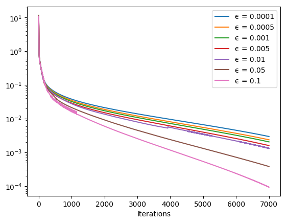
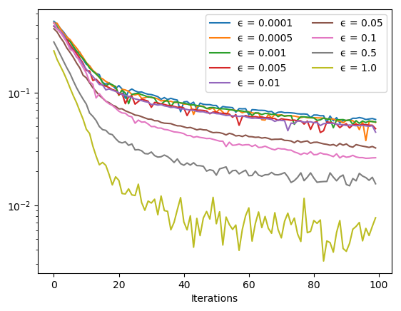
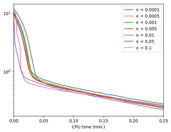
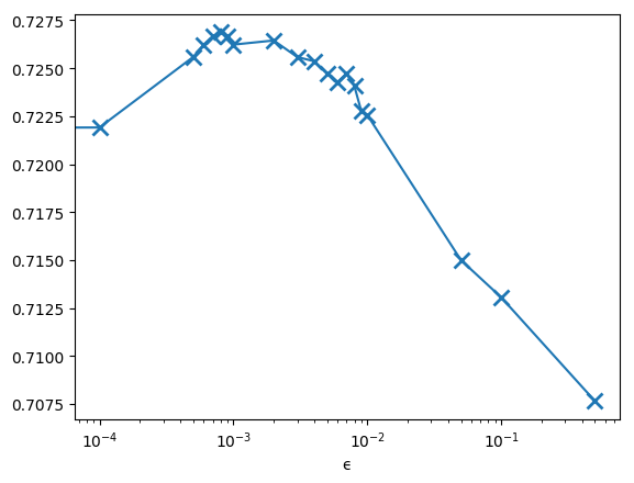
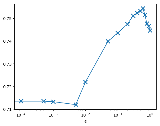
Figure 3 shows the value of the area under the ROC curve (AUC metric) Bradley (1997) as a function of $\epsilon$, computed using the testing set. There is a clear compromise in the choice of the value of $\epsilon$ for maximizing the AUC, and the best performance are obtained for an intermediate non-zero value of this parameter. This clearly illustrates the benefit of the proposed formulation. Note that such results are consistent with the conclusions in Shafieezadeh-Abadeh, Esfahani, and Kuhn (2015) and Gotoh, Kim, and Lim (2018). On this example, the Wassertein ambiguity set provides better results than the Kullback-Leibler divergence but it should be reminded that it comes at the expense of a higher computational cost.

(a) Kullback-Leibler divergence

(b) Wasserstein distance

Figure 3: ionosphere dataset: AUC metric as a function of $\epsilon$.

6.2.2 Colon-cancer dataset

We now present in Table 2 the evolution of the AUC for tests performed on the colon-cancer dataset. This dataset only contains 64 observations. For such small dataset, the formulation in Problem 12 becomes very cheap in terms of computational cost. As can be noticed in Table 2, taking a nonzero value for $\epsilon$ leads to an increase of about 7% in terms AUC, which is significant in such challenging context. These results allow to assess the robustness property of the proposed formulation.

Value of $\epsilon$	AUC with KL	AUC with Wasserstein
$\epsilon=0$ (LR)	0.832	0.832
$\epsilon=0.001$	0.757	0.787
$\epsilon=0.002$	0.750	0.770
$\epsilon=0.003$	0.779	0.706
$\epsilon=0.004$	0.698	0.691
$\epsilon=0.005$	0.868	0.831
$\epsilon=0.006$	0.890	0.860
$\epsilon=0.007$	0.728	0.838
$\epsilon=0.008$	0.809	0.768
$\epsilon=0.009$	0.875	0.890
$\epsilon=0.01$	0.801	0.853
$\epsilon=0.05$	0.786	0.794
$\epsilon=0.1$	0.801	0.816

Table 2: colon-cancer dataset: Values of the AUC for different values of $\epsilon$.

6.3 Results on an altered database

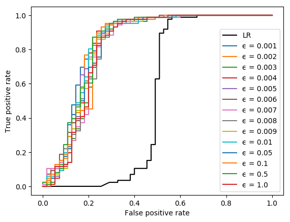
Let us come back to the processing of ionosphere dataset. In order to better illustrate the interest of the proposed formulation, we propose to modify the training set so that the proportion of labels $(-1)$ and $(+1)$ is altered and unbalanced. Such situation could typically arise during a transient regime, such as the beginning of an epidemic, or in the case of an incomplete dataset. After dividing the dataset between a training set and a testing set, using the same 60% ratio as in our previous tests, we will drop randomly a certain number of observations associated with the label $(-1)$ so that the proportion of this label becomes ten times lower than its original proportions. Figure 4 displays ROC curves and Table 3 evaluates AUC metric, for various values of $\epsilon$. Our formulation clearly outperforms the classical logistic regression classifier (retrieved when $\epsilon=0)$. Noticeably, the later presents the same area under the curve as a random classifier, and thus exhibits a similar behavior to such a classifier.

(a) Kullback-Leibler divergence

(b) Wasserstein distance

Figure 4: ionosphere dataset (altered): ROC curve for different values of $\epsilon$.

Value of $\epsilon$	AUC with KL	AUC with Wasserstein
$\epsilon=0$ (LR)	0.514	0.514
$\epsilon=0.001$	0.816	0.840
$\epsilon=0.002$	0.804	0.835
$\epsilon=0.003$	0.840	0.814
$\epsilon=0.004$	0.824	0.830
$\epsilon=0.005$	0.815	0.829
$\epsilon=0.006$	0.834	0.829
$\epsilon=0.007$	0.821	0.815
$\epsilon=0.008$	0.835	0.815
$\epsilon=0.009$	0.823	0.822
$\epsilon=0.01$	0.828	0.835
$\epsilon=0.05$	0.815	0.826
$\epsilon=0.1$	0.824	0.823

Table 3: ionosphere dataset (altered): Values of the area under ROC curve for different values of $\epsilon$.

6.4 Variance reduction study

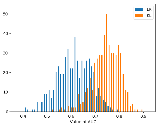
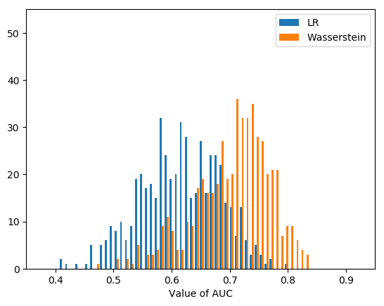
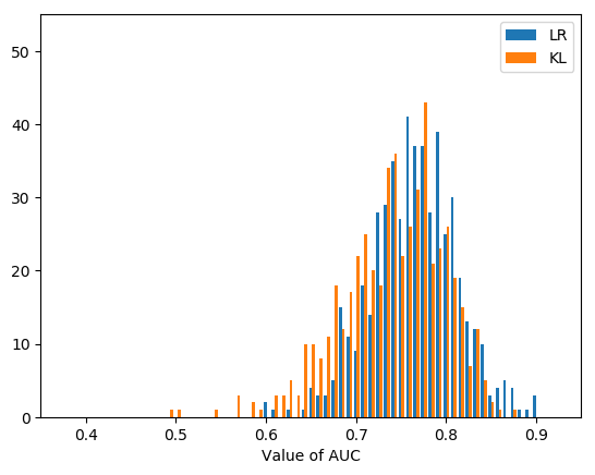
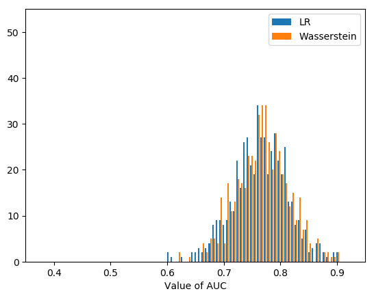
In a nutshell, the robust framework based on the Wasserstein distance provides a better expected reward but at the expense of a higher computational cost. The risk measure based on the Kullback-Leibler divergence is easily tractable, provides a reduction of the variance in out-of-samples results, but a smaller increase in terms of expected reward (see  Gotoh, Kim, and Lim (2018) for a more detailed theoretical analysis). In practice, as discussed in  Shafieezadeh-Abadeh, Esfahani, and Kuhn (2015) and in Gotoh, Kim, and Lim (2018), “a little of robustness” typically improves a bit the expected reward (around 1%), however results in a larger reduction in terms of variance. We propose to reproduce such an analysis by means of two experiments using ionosphere dataset. We first consider the case when a small training set is used where only 10% of the data are available. Then we focus on the case when 60% of the data are used as training set. In both cases, 1000 random realizations are run, when we solve the classical formulation using logistic regression (LR) loss in Equation (2), the formulation in Problem 9 that uses ambiguity sets defined through the Kullback-Leibler divergence, and the formulation in Problem 12 that uses ambiguity sets defined through the Wasserstein distance. We then compute the value of the AUC metric on the associated testing set and display results as histograms. When we use 10% of the data for training (Figure 5), we see the benefits of our robust solution with respect to the standard LR classifier. When more data are collected, the probability distribution becomes more accurate and our robust models tend to produce the same outputs as when using classical logistic regression (Figure 6).

(a) Kullback-Leibler divergence

(b) Wasserstein distance

Figure 5: ionosphere dataset: AUC histogram for 1000 random realizations using 10% of data for the training set. Robust model is used with $\epsilon=0.001$.

(a) Kullback-Leibler divergence

(b) Wasserstein distance

Figure 6: ionosphere dataset: AUC histogram for 1000 random realizations using 60% of data for the training set. Robust model is used with $\epsilon=0.001$.

7 Conclusion

We have highlighted that risk measures offer versatile tools for addressing machine learning problems in a robust manner. By assuming that the loss function is convex, the related optimization problem has been recast as a convex one. We have shown that various classes of risk measures, e.g. those based on $\varphi$-divergences or on the Wasserstein distance, lead to a common convex formulation. In addition, an efficient convex optimization algorithm has been proposed to cope with the non trivial constrained problem resulting from this formulation. We have conducted numerical experiments in which various ambiguity sets are tackled thanks to the same algorithm. We have also illustrated that the considered robust models can outperform classical ones in challenging contexts when the size of the training set is limited, or when the distribution of labels in the training set is not representative of the reality.

References

- Ali and Silvey (1966) S. M. Ali and S. D. Silvey. A general class of coefficients of divergence of one distribution from another. Journal of the Royal Statistical Society. Series B (Methodological), pages 131–142, 1966.
- Artzner et al. (1999) P. Artzner, F. Delbaen, J.-M. Eber, and D. Heath. Coherent measures of risk. Mathematical finance, 9(3):203–228, 1999.
- Basseville (2013) M. Basseville. Divergence measures for statistical data processing—an annotated bibliography. Signal Processing, 93(4):621–633, 2013.
- Bauschke and Combettes (2011) H. H. Bauschke and P. L. Combettes. Convex Analysis and Monotone Operator Theory in Hilbert Spaces. Springer, New York, 2011.
- Beck and Teboulle (2009) A. Beck and M. Teboulle. A fast iterative shrinkage-thresholding algorithm for linear inverse problems. SIAM Journal on Imaging Sciences, 2(1):183–202, 2009.
- Ben-Tal and Nemirovski (2000) A. Ben-Tal and A. Nemirovski. Robust solutions of linear programming problems contaminated with uncertain data. Mathematical programming, 88(3):411–424, 2000.
- Ben-Tal et al. (2009) A. Ben-Tal, L. El Ghaoui, and A. Nemirovski. Robust optimization. Princeton University Press, 2009.
- Ben-Tal et al. (2013) A. Ben-Tal, D. Den Hertog, A. De Waegenaere, B. Melenberg, and G. Rennen. Robust solutions of optimization problems affected by uncertain probabilities. Management Science, 59(2):341–357, 2013.
- Bradley (1997) A. P. Bradley. The use of the area under the roc curve in the evaluation of machine learning algorithms. Pattern recognition, 30(7):1145–1159, 1997.
- Briceno-Arias et al. (2017) L. M. Briceno-Arias, G. Chierchia, E. Chouzenoux, and J.-C. Pesquet. A random block-coordinate douglas-rachford splitting method with low computational complexity for binary logistic regression. arXiv preprint arXiv:1712.09131, 2017.
- Chambolle and Dossal (2015) A. Chambolle and C. Dossal. Journal of Optimization Theory and Applications, 166(3):968–982, 2015.
- Combettes (2000) P. L. Combettes. Strong convergence of block-iterative outer approximation methods for convex optimization. SIAM Journal on Control and Optimization, 38(2):538–565, 2000.
- Combettes (2003) P. L. Combettes. A block-iterative surrogate constraint splitting method for quadratic signal recovery. IEEE Transactions on Signal Processing, 51(7):1771–1782, 2003.
- Combettes and Müller (2018) P. L. Combettes and C. L. Müller. Perspective functions: Proximal calculus and applications in high-dimensional statistics. Journal of Mathematical Analysis and Applications, 457(2):1283–1306, 2018.
- Combettes and Pesquet (2010) P. L. Combettes and J.-C. Pesquet. Proximal splitting methods in signal processing. In H. H. Bauschke, R. Burachik, P. L. Combettes, V. Elser, D. R. Luke, and H. Wolkowicz, editors, Fixed-Point Algorithms for Inverse Problems in Science and Engineering, pages 185–212. Springer-Verlag, New York, 2010.
- Combettes et al. (2010) P. L. Combettes, D. Dung, and B. C. Vũ. Dualization of signal recovery problems. Set-Valued and Variational Analysis, 18(3):373–404, Dec. 2010.
- Csiszár (1964) I. Csiszár. Eine informationstheoretische ungleichung und ihre anwendung auf beweis der ergodizitaet von markoffschen ketten. Magyer Tud. Akad. Mat. Kutato Int. Koezl., 8:85–108, 1964.
- Duchi et al. (2016) J. Duchi, P. Glynn, and H. Namkoong. Statistics of robust optimization: A generalized empirical likelihood approach. arXiv preprint arXiv:1610.03425, 2016.
- Esfahani and Kuhn (2015) P. M. Esfahani and D. Kuhn. Data-driven distributionally robust optimization using the wasserstein metric: Performance guarantees and tractable reformulations. arXiv preprint arXiv:1505.05116, 2015.
- Esfahani et al. (2017) P. M. Esfahani, S. Shafieezadeh-Abadeh, G. A. Hanasusanto, and D. Kuhn. Data-driven inverse optimization with imperfect information. Mathematical Programming, pages 1–44, 2017.
- Feng et al. (2014) J. Feng, H. Xu, S. Mannor, and S. Yan. Robust logistic regression and classification. In Advances in neural information processing systems, pages 253–261, 2014.
- Föllmer and Schied (2016) H. Föllmer and A. Schied. Stochastic finance: an introduction in discrete time (4th edition). Walter de Gruyter, 2016.
- Gotoh et al. (2018) J.-y. Gotoh, M. J. Kim, and A. E. Lim. Robust empirical optimization is almost the same as mean–variance optimization. Operations Research Letters, 2018.
- Haugazeau (1968) Y. Haugazeau. Sur les inéquations variationnelles et la minimisation de fonctionnelles convexes. These, Universite de Paris, 1968.
- Hu and Hong (2013) Z. Hu and L. J. Hong. Kullback-leibler divergence constrained distributionally robust optimization. Available at Optimization Online, 2013.
- Kurakin et al. (2016) A. Kurakin, I. Goodfellow, and S. Bengio. Adversarial examples in the physical world. arXiv preprint arXiv:1607.02533, 2016.
- Moghaddam and Mahlooji (2016) S. Moghaddam and M. Mahlooji. Robust simulation optimization using -divergence. International Journal of Industrial Engineering Computations, 7(4):517–534, 2016.
- Morimoto (1963) T. Morimoto. Markov processes and the h-theorem. Journal of the Physical Society of Japan, 18(3):328–331, 1963.
- Namkoong and Duchi (2016) H. Namkoong and J. C. Duchi. Stochastic gradient methods for distributionally robust optimization with f-divergences. In Advances in Neural Information Processing Systems, pages 2208–2216, 2016.
- Papernot et al. (2016) N. Papernot, P. McDaniel, and I. Goodfellow. Transferability in machine learning: from phenomena to black-box attacks using adversarial samples. arXiv preprint arXiv:1605.07277, 2016.
- Plan and Vershynin (2013) Y. Plan and R. Vershynin. Robust 1-bit compressed sensing and sparse logistic regression: A convex programming approach. IEEE Transactions on Information Theory, 59(1):482–494, 2013.
- Rockafellar and Uryasev (2000) R. T. Rockafellar and S. Uryasev. Optimization of conditional value-at-risk. Journal of risk, 2:21–42, 2000.
- Ruszczyński and Shapiro (2006) A. Ruszczyński and A. Shapiro. Conditional risk mappings. Mathematics of operations research, 31(3):544–561, 2006.
- Ruszczynski and Shapiro (2006) A. Ruszczynski and A. Shapiro. Optimization of convex risk functions. Mathematics of operations research, 31(3):433–452, 2006.
- Shafieezadeh-Abadeh et al. (2015) S. Shafieezadeh-Abadeh, P. M. Esfahani, and D. Kuhn. Distributionally robust logistic regression. In Advances in Neural Information Processing Systems, pages 1576–1584, 2015.