Computing the volume of compact semi-algebraic sets

Abstract.

Let $S\subset{\mathbb{R}}^{n}$ be a compact basic semi-algebraic set defined as the real solution set of multivariate polynomial inequalities with rational coefficients. We design an algorithm which takes as input a polynomial system defining $S$ and an integer $p\geqslant 0$ and returns the $n$-dimensional volume of $S$ at absolute precision $2^{-p}$.

Our algorithm relies on the relationship between volumes of semi-algebraic sets and periods of rational integrals. It makes use of algorithms computing the Picard-Fuchs differential equation of appropriate periods, properties of critical points, and high-precision numerical integration of differential equations.

The algorithm runs in essentially linear time with respect to $p$. This improves upon the previous exponential bounds obtained by Monte-Carlo or moment-based methods. Assuming a conjecture of Dimca, the arithmetic cost of the algebraic subroutines for computing Picard-Fuchs equations and critical points is singly exponential in $n$ and polynomial in the maximum degree of the input.

1. Introduction

Semi-algebraic sets are the subsets of ${\mathbb{R}}^{n}$ which are finite unions of real solution sets to polynomial systems of equations and inequalities with coefficients in ${\mathbb{R}}$. Starting from Tarski’s algorithm for quantifier elimination (Tarski, 1998) improved by Collins through the Cylindrical Algebraic Decomposition algorithm (Collins, 1975), effective real algebraic geometry yields numerous algorithmic innovations and asymptotically faster routines for problems like deciding the emptiness of semi-algebraic sets, answering connectivity queries or computing Betti numbers (e.g., Basu et al., 2006; Safey El Din and Schost, 2003; Canny, 1988; Safey El Din and Schost, 2017; Bürgisser et al., 2019). The output of all these algorithms is algebraic in nature. In this paper, we study the problem of computing the volume of a (basic) compact semi-algebraic set $S\subset{\mathbb{R}}^{n}$ defined over ${\mathbb{Q}}$. The output may be transcendental: for instance, the area of the unit circle in ${\mathbb{R}}^{2}$ is $\pi$.

Volumes of semi-algebraic sets actually lie in a special class of real numbers, for they are closely related to Kontsevich-Zagier periods introduced in (Kontsevich and Zagier, 2001). A (real) period is the value of an absolutely convergent integral of a rational function with rational coefficients over a semi-algebraic set defined by polynomials with rational coefficients. For example, algebraic numbers are periods, as are $\pi$, $\log 2$, $\zeta(3)$. Since $\operatorname{vol}S=\int_{S}1\mathrm{d}x$, volumes of semi-algebraic sets defined over ${\mathbb{Q}}$ are periods. Conversely, interpreting an integral as a “volume under a graph” shows that periods are differences of volumes of semi-algebraic sets defined over ${\mathbb{Q}}$. In (Viu-Sos, 9 03), it is further shown that periods are differences of volumes of compact semi-algebraic sets defined over ${\mathbb{Q}}$.

The problem we consider in this paper is thus a basic instance of the more general problem of integrating an algebraic function over a semi-algebraic set; it finds applications in numerous areas of engineering sciences. Performing these computations at high precision (hundreds to thousands of digits) is also relevant in experimental mathematics, especially for discovering formulas, as explained, for example, in (Bailey and Borwein, 2011). Most of the examples featured in this reference are periods, sometimes in disguise.

Prior work.

The simplest semi-algebraic sets one can consider are polytopes. The computation of their volume has been extensively studied, with a focus on the complexity with respect to the dimension. It is known that even approximating the volume of a polytope deterministically is #P-hard (Dyer and Frieze, 1988; Khachiyan, 1989). The celebrated probabilistic approximation algorithm in (Dyer et al., 1991), which applies to more general convex sets, computes an $\varepsilon$-approximation in time polynomial in the dimension of the set and $1/\varepsilon$. A key ingredient for this algorithm is a Monte Carlo method for efficiently sampling points from a convex set. Since then, Monte Carlo schemes have been adopted as the framework of several volume estimation algorithms.

In contrast, we deal here with compact semi-algebraic sets which can be non-convex and even non-connected. Additionally, while volumes of polytopes are rational, the arithmetic nature of volumes of semi-algebraic sets is much less clear, as unclear as the nature of periods. This raises the question of the computational complexity of a volume, even taken as a single real number.

A simple Monte Carlo technique applies in our setting as well: one samples points uniformly in a box containing $S$ and estimates the probability that they lie in $S$. This method is of practical interest at low precision but requires $2^{\Omega(p)}$ samples to achieve an error bounded by $2^{-p}$ with high probability. We refer to (Koiran, 1995) which deals with definable sets, a class which encompasses semi-algebraic sets.

In a different direction, numerical approximation schemes based on the moment problem and semi-definite programming have been designed in (Henrion et al., 2009). They are also of practical interest at low precision, and can provide rigorous error bounds, but the convergence is worse than exponential with respect to $p$ (Korda and Henrion, 2018).

Another line of research, going back to the nineteenth century, is concerned with the computation of periods of algebraic varieties. In particular, we build on work (Chudnovsky and Chudnovsky, 1990) on the high-precision numerical solution of ODEs with polynomial coefficients which was motivated, among other things, by applications to periods of Abelian integrals (see Chudnovsky and Chudnovsky, 1990, p. 133).

Main result.

We describe a new strategy for computing volumes of semi-algebraic sets, at the crossroads of effective algebraic and real algebraic geometry, symbolic integration, and rigorous numerical computing. Our approach effectively reduces the volume computation to the setting of (Chudnovsky and Chudnovsky, 1990). It yields an algorithm that approximates the volume of a fixed, bounded basic semi-algebraic set in almost linear time with respect to the precision. More precisely, we prove the following bit complexity estimate.

Theorem 1.

Let $f_{1},\ldots,f_{r}$ be polynomials in ${\mathbb{Q}}[x_{1},\ldots,x_{n}]$, and let $S\subset{\mathbb{R}}^{n}$ be the semi-algebraic set defined by $f_{1}\geqslant 0,\ldots,f_{r}\geqslant 0$. Assume that $S$ is compact. There exists an algorithm which computes, on input $p\geqslant 0$ and $(f_{1},\ldots,f_{r})$, an approximation $\tilde{V}$ of the volume $V$ of $S$ with $|\tilde{V}-V|\leqslant 2^{-p}$. When $f_{1},\dots,f_{r}$ are fixed, the algorithm runs in time $O(p\log(p)^{3+\varepsilon})$ (for any $\varepsilon>0$) as $p\to\infty$.

The algorithm recursively computes integrals of volumes of sections of $S$. Let $v(t)$ denote the $(n-1)$-dimensional volume of $S\cap\mathrm{pr}^{-1}(t)$, for some nonzero linear projection $\mathrm{pr}:{\mathbb{R}}^{n}\to{\mathbb{R}}$. In our setting, $v$ is a piecewise analytic function and, except at finitely many $t$, is solution of a linear differential equation with polynomial coefficients known as a Picard-Fuchs equation.

The problem points belong to the critical locus of the restriction of the projection $\mathrm{pr}$ to a certain hypersurface containing the boundary of $S$ and are found by solving appropriate polynomial systems. (Compare (Khachiyan, 1993) in the case of polytopes.) The Picard-Fuchs equation for $v$ is produced by algorithms from symbolic integration, in particular (Bostan et al., 2013; Lairez, 2016). To obtain the volume of $S$, it then suffices to compute $\int_{\mathbb{R}}v$ with a rigorous numerical ODE solving algorithm, starting from values $v(\rho_{i})$ at suitable points $\rho_{i}$ obtained through recursive calls.

The complexity with respect to the dimension $n$ of the ambient space and the number $r$, maximum degree $D$, and coefficient size of the polynomials $f_{i}$ is harder to analyze. We will see, though, that under reasonable assumptions, the “algebraic” steps (computing the critical loci and of the Picard-Fuchs equations) take at most $(rD)^{O(n^{2})}$ arithmetic operations in ${\mathbb{Q}}$.

Example.

The idea of the method is well illustrated by the example of a torus $S$, here of major radius $2$ and minor radius $1$. Let

$$S=\left\{(x,y,z)\in{\mathbb{R}}^{3}\ \middle|\ (x^{2}+y^{2}+z^{2}+3)^{2}\leqslant 16(x^{2}+y^{2})\right\}.$$

The area (2-dimensional volume) of a section $S\cap\left\{x=t\right\}$ defines a function $v:{\mathbb{R}}\to{\mathbb{R}}$ (see Figure 1).

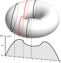
Figure 1. Volume of the sections of the torus $S$ as a function of the parameter $t$. In red, a singular section.

It is analytic, except maybe at the critical values $t=\pm 3$ and $t=\pm 1$ where the real locus of the curve $(t^{2}+y^{2}+z^{2}+3)^{2}=16(t^{2}+y^{2})$ is singular. On each interval on which $v$ is analytic, it satisfies the Picard-Fuchs equation

(1) $$(t-3)(t+3)(t-1)^{2}(t+1)^{2}t^{2}v^{\prime\prime\prime}(t)+(t^{2}+9)(t-1)^{2}(t+1)^{2}tv^{\prime\prime}(t)\\ -(2t^{4}+11t^{2}-9)(t-1)(t+1)v^{\prime}(t)+2(t^{2}+3)t^{3}v(t)=0,$$

which we compute in 2 seconds on a laptop using the algorithm of (Lairez, 2016) and Theorem 8.

We know some special values of $v$, namely $v(0)=2\pi$, $v(\pm 1)=8$ and $v(\pm 3)=0$. Additionally, we have $v(3\pm t)=O(t^{2})$ as $t\to\mp 0$. These properties characterize the analytic function $v_{|(-1,1)}$ in the $2$-dimensional space of analytic solutions of the differential equation (1) on $(-1,1)$, and similarly for $v_{|(1,3)}$. (Our algorithm actually uses recursive calls at generic points instead of these ad hoc conditions.) The rigorous ODE solver part of the Sage package ore_algebra (Mezzarobba, 2016) determines in less than a second that

$$\int_{-3}^{3}v(t)\mathrm{d}t=39.4784176043[...]25056533975\pm 10^{-60}.$$

And indeed, it is not hard to see in this case that $\operatorname{vol}S=4\pi^{2}$. We can obtain 1000 digits in less than a minute.

Outline.

The remainder of this article is organized as follows. In Section 2, we give a high-level description of the main algorithm. As sketched above, the algorithm relies on the computation of critical points, Picard-Fuchs equations, and numerical solutions of these equations. In Section 3, we discuss the computation of Picard-Fuchs equations and critical points, relating these objects with analyticity properties of the “section volume” function. Then, in Section 4, we describe the numerical solution process and study its complexity with respect to the precision. Finally, in Section 5, we conclude the proof of Theorem 1 and state partial results on the complexity of the algorithm with respect to $n$, $r$, and $D$.

Acknowledgements.

We would like to thank the anonymous reviewers for their careful reading and valuable comments.

2. Volumes of semi-algebraic sets

We start by designing an algorithm which deals with the case of a union of connected components of a semi-algebraic set defined by a single inequality. Next, we will use a deformation technique to handle semi-algebraic sets defined by several inequalities.

2.1. Sets defined by a single inequality

Let $f\in{\mathbb{Q}}[t,x_{1},\dotsc,x_{n}]$ and $A$ be the semi-algebraic set

$$A\triangleq\left\{(\rho,x)\in{\mathbb{R}}\times{\mathbb{R}}^{n}\ \middle|\ f(\rho,x)\geqslant 0\right\}.$$

Let $\mathrm{pr}:{\mathbb{R}}^{n+1}\to{\mathbb{R}}$ be the projection on the $t$-coordinate. We want to compute the volume of a union $U$ of connected components of $A$ starting from the volumes of suitable fibers $U\cap\mathrm{pr}^{-1}(\rho)$. For technical reasons, we first consider the slightly more general situation where $U$ is a union of connected components of $A\cap\mathrm{pr}^{-1}(I)$ for some open interval $I\subseteq{\mathbb{R}}$. From a computational point of view, we assume that $U$ is described by a semi-algebraic formula $\Theta_{U}$, that is,

$$U=\left\{(\rho,x)\in A\ \middle|\ \Theta_{U}(\rho,x)\right\},$$

where $\Theta_{U}$ is a finite disjunction of conjunctions of polynomial inequalities with (in our setting) rational coefficients.

For $\rho\in I$, let $U_{\rho}\triangleq U\cap\mathrm{pr}^{-1}(\rho)$ and $v(\rho)\triangleq\operatorname{vol}_{n}U_{\rho}$. Let $\Sigma_{f}\subseteq{\mathbb{R}}$ (we will often omit the subscript $f$) be the set of exceptional values

(2) $$\Sigma_{f}\triangleq\left\{\rho\in{\mathbb{R}}\mid\exists x\in{\mathbb{R}}^{n},f(\rho,x)=0\wedge\forall i,\tfrac{\partial}{\partial x_{i}}f(\rho,x)=0\right\}.$$

Thus, when $f$ is square-free, exceptional values are either critical values of the restriction to the hypersurface $\{f=0\}$ of the projection $\mathrm{pr}$, or images of singular points of $\{f=0\}$. By definition of $\Sigma$, for any $\rho\in{\mathbb{R}}\setminus\Sigma$, the zero set of $f_{\rho}=f(\rho,-)$ is a smooth submanifold of ${\mathbb{R}}^{n}$.

Further, we say that assumption (R) holds for $f$ if

(R) $$\left\{z\in\mathbb{R}^{n+1}\ \middle|\ f(z)=0\wedge\tfrac{\partial}{\partial t}f(z)=0\wedge\forall i,\tfrac{\partial}{\partial x_{i}}f(z)=0\right\}=\varnothing.$$

Observe that by Sard’s theorem (e.g. Basu et al., 2006, Theorem 5.56), when (R) holds, the exceptional set $\Sigma$ is finite.

The mainstay of the method is the next result, to be proved in §3. Let $\mathscr{D}\subset{\mathbb{Q}}[t][\frac{\mathrm{d}}{\mathrm{d}t}]$ denote the set of Fuchsian linear differential operators with coefficients in ${\mathbb{Q}}[t]$ whose local exponents at singular points are rational (see §4 for reminders on Fuchsian operators and their exponents).

Theorem 2.

If $U$​ is bounded and $I\cap\Sigma=\varnothing$, then the function $v_{|I}$ is solution of a computable differential equation of the form $P(v)=0$, where $P\in\mathscr{D}$ depends only on $f$.

We will also use the following proposition, which summarizes the results of Proposition 12 and Lemma 13 in §4. The complete definition of “good initial conditions” is given there as well. Up to technical details, this simply means a system $\mathscr{I}$ of linear equations of the form $y^{(k)}(u)=s$ that suffices to characterize a particular solution $y$ among the solutions of $P(y)=0$. An $\varepsilon$-approximation of $\mathscr{I}$ is made of the same equations with each right-hand side $s$ replaced by an enclosure $\tilde{s}\ni s$ of diameter $\leqslant\varepsilon$.

Proposition 2.

Let $P\in\mathscr{D}$ have order $m$, and let $J=(\alpha,\beta)$ be a real interval with algebraic endpoints. Let $y:J\to{\mathbb{R}}$ be a solution of $P(y)=0$ with a finite limit at $\alpha$ and $\mathscr{I}$ be a system of good initial conditions for $P$ on $J$ defining $y$.

1. Given $P,\alpha$, a precision $p\in{\mathbb{N}}$ and a $2^{-p}$-approximation $\tilde{\mathscr{I}}$ of $\mathscr{I}$, one can compute an interval of width $O(2^{-p})$ (as $p\to\infty$ for fixed $P$, $\alpha$, and $\mathscr{I}$) containing $\lim_{t\to\alpha}y(t)$.

2. Given $P,\alpha,\beta$, one can compute $\rho_{1},\dots,\rho_{m}\in J\cap{\mathbb{Q}}$ such that the $y(\rho_{j})$ form a system of good initial conditions for $P$ on $J$.

Assume now that $U$ is a bounded union of connected components of $A$ (i.e., that we can take $I={\mathbb{R}}$ above), and that (R) holds for $f$. The algorithm is recursive. Starting with input $f,\Theta_{U}$, and $p$, it first computes the set $\Sigma=\{\alpha_{1}\leqslant\cdots\leqslant\alpha_{\ell}\}$ of exceptional values so as to decompose ${\mathbb{R}}-\Sigma$ into intervals over which the function $v$ satisfies the differential equation $P(y)=0$ given by Theorem 2. Since $U$ is bounded, one has

$$\operatorname{vol}_{n+1}U=\sum_{i=1}^{\ell-1}\operatorname{vol}_{n+1}\left(U\cap\mathrm{pr}^{-1}(\alpha_{i},\alpha_{i+1})\right)=\sum_{i=1}^{\ell-1}\int_{\alpha_{i}}^{\alpha_{i+1}}v(t)\,\mathrm{d}t.$$

Fix $i$ and consider the interval $J=(\alpha_{i},\alpha_{i+1})$. Since $v_{|J}$ is annihilated by $P$, its anti-derivative $w:J\to{\mathbb{R}}$ vanishing at $\alpha_{i+1}$ is annihilated by the operator $P\,\frac{\mathrm{d}}{\mathrm{d}t}$, which belongs to $\mathscr{D}$ since $P$ does. Additionally, if $[v(\rho_{j})=s_{j}]_{j}$ is a system of good initial conditions for $P$ that defines $v_{|J}$, then $[w^{\prime}(\rho_{j})=s_{j}]_{j}\cup[w(\alpha_{i+1})=0]$ is a system of good initial conditions for $P\,\frac{\mathrm{d}}{\mathrm{d}t}$ defining $w$ (see Lemma 12 in §4). Thus, by Proposition 2, to compute $w(\alpha_{i})$ to absolute precision $p$, it suffices to compute $v(\rho_{j})$, $1\leqslant j\leqslant m$, to precision $p+O(1)$.

By definition of $\Sigma$, since $\rho_{j}\notin\Sigma$, there is no solution to the system

$$f(\rho_{j},-)=\tfrac{\partial}{\partial x_{1}}f(\rho_{j},-)=\cdots=\tfrac{\partial}{\partial x_{n}}f(\rho_{j},-)=0$$

which means that (R) holds for $f(\rho_{j},-)$. Additionally, $U\cap\mathrm{pr}^{-1}(\rho_{j})$ is a bounded union of connected components of $A\cap\mathrm{pr}^{-1}(\rho_{j})$. Hence, the values $v(\rho_{j})$ can be obtained by recursive calls to the algorithm with $t$ instantiated to $\rho_{j}$.

The process terminates since each recursive call handles one less variable. In the base case, we are left with the problem of computing the length of a union of real intervals encoded by a semi-algebraic formula. This is classically done using basic univariate polynomial arithmetic and real root isolation (Basu et al., 2006, Chap. 10).

Algorithm 1 Volume of $U$ at precision $O(2^{-p})$

1:procedure Volume1($f,\Theta_{U},(t,x_{1},\ldots,x_{n}),p$)

2:     if $n=0$ then return $\textsc{UnivariateVolume}(f,\Theta_{U},p)$.      

3:     $(\alpha_{1},\ldots,\alpha_{\ell})\leftarrow\textsc{CriticalValues}(f,t)$

4:     $P\leftarrow\textsc{PicardFuchs}(f,t)$

5:     for $1\leqslant i\leqslant\ell-1$ do $\triangleright$ $\tilde{s}_{j}$, $\tilde{S}_{i}$ are intervals

6:         $(\rho_{1},\ldots,\rho_{m})\leftarrow\textsc{PickGoodPoints}(P,\alpha_{i},\alpha_{i+1})$

7:         for $1\leqslant j\leqslant m$ do

8:              $\tilde{s}_{j}\leftarrow\textsc{Volume1}(f_{|t=\rho_{j}},{\Theta_{U}}_{|t=\rho_{j}},(x_{1},\ldots,x_{n}),p)$          

9:         $\tilde{\mathscr{I}}\leftarrow[y^{\prime}(\rho_{1})=\tilde{s}_{1},\dots,y^{\prime}(\rho_{m})=\tilde{s}_{m},y(\alpha_{i+1})=0]$

10:         $\tilde{S}_{i}\leftarrow-\textsc{DSolve}(P\frac{\mathrm{d}}{\mathrm{d}t},\tilde{\mathscr{I}},\alpha_{i},p)$      

11:     return $\tilde{S}_{1}+\cdots+\tilde{S}_{\ell}$

The complete procedure is formalized in Algorithm 1. The quantities denoted with a tilde in the pseudo-code are understood to be represented by intervals, and the operations involving them follow the semantics of interval arithmetic. Additionally, we assume that we have at our disposal the following subroutines:

• $\textsc{PicardFuchs}(f,t)$, $\textsc{DSolve}(P,\tilde{\mathscr{I}},\alpha,p)$, and $\textsc{PickGoodPoi}\linebreak[0]\textsc{nts}(P,\alpha,\beta)$, which implement the algorithms implied, respectively, by Theorem 2 and Proposition 2 (1) and (2);

• $\textsc{CriticalValues}(f,t)$, which returns an encoding for a finite set of real algebraic numbers containing the exceptional values associated to $f$, sorted in increasing order;

• $\textsc{UnivariateVolume}(g,\Theta_{U},p)$ where $g\in{\mathbb{Q}}[t]$ and $\Theta_{U}$ is a semi-algebraic formula describing a union $U$ of connected components of $\{g\geqslant 0\}$, which returns an interval of width $\leqslant 2^{-p}$ containing $\operatorname{vol}_{1}U$.

The following result summarizes the above discussion.

Theorem 3.

Assume that $U$ is a bounded union of connected components of $A$ and that (R) holds. Then, on input $f,\Theta_{U},p$ and $(t,x_{1},\ldots,x_{n})$, Algorithm 1 (Volume1) returns a real interval of width $O(2^{-p})$ (for fixed $f$) containing $\operatorname{vol}_{n+1}U$.

2.2. Sets defined by several inequalities

Now, we show how to compute the volume of a basic semi-algebraic set $S\subset{\mathbb{R}}^{n}$ defined by

$$f_{1}\geqslant 0,\ldots,f_{r}\geqslant 0,\qquad f_{i}\in{\mathbb{Q}}[x_{1},\dots,x_{n}],$$

assuming that $S$ is compact.

We set $f=f_{1}\cdots f_{r}-t\in{\mathbb{Q}}[t,x_{1},\dots,x_{n}]$, and consider the semi-algebraic set $A\subset{\mathbb{R}}^{n+1}$ defined by $f\geqslant 0$. Observe that the polynomial $f$ satisfies (R) because $\frac{\partial f}{\partial t}=-1$. We can hence choose an interval $I=(0,\alpha)$ with $\alpha\in{\mathbb{Q}}$ that contains no element of $\Sigma_{f}$. Let $U\triangleq A\cap(I\times S)$ and $\mathrm{pr}$ be the projection on the $t$-coordinate. For fixed $\rho\in I$, the set $U\cap\mathrm{pr}^{-1}(\rho)$ can be viewed as a bounded subset of $S$, whose volume $v(\rho)=\operatorname{vol}_{n}(U\cap\mathrm{pr}^{-1}(\rho))$ tends to $\operatorname{vol}_{n}S$ as $\rho\to 0$.

The set $U$ itself is bounded and the formula

$$\Theta_{U}=f_{1}\geqslant 0\wedge\dotsb\wedge f_{r}\geqslant 0\wedge 0<t<\alpha$$

defines $U$ in $A$. In addition, $U$ is a union of connected components of $A\cap\mathrm{pr}^{-1}(I)$. Indeed, for any point $(\rho,x)\in A$ with $\rho\in I$, it holds that $f_{1}(x)\dotsb\allowbreak f_{r}(x)>0$. This implies that $U=A\cap(I\times\mathring{S})$ where $\mathring{S}$ is the interior of $S$. Therefore, $U$ is both relatively closed (as the trace of ${\mathbb{R}}\times S$) and open (as that of ${\mathbb{R}}\times\mathring{S}$) in $A\cap\mathrm{pr}^{-1}(I)$.

We are hence in the setting of the previous subsection. Since $I\cap\Sigma_{f}=\varnothing$ by definition of $I$, Theorem 2 applies, and the function $v:I\to{\mathbb{R}}$ is annihilated by an operator $P\in\mathscr{D}$ which is computed using the routine PicardFuchs introduced earlier. By Proposition 2, one can choose rational points $\rho_{j}\in I$ such that the values of $v$ at these points characterize it among the solutions of $P$, and, given sufficiently precise approximations of $v(\rho_{j})$, one can compute $\operatorname{vol}_{n}S=\lim_{t\to 0}v(t)$ to any desired accuracy.

The “initial conditions” $v(\rho_{j})$ are computed by calls to Algorithm 1 with $f$ and $\Theta_{U}$ specialized to $t=\rho_{j}$. In the notation of §2.1, this corresponds to taking $A=A(\rho_{j})=\{f_{1}\cdots f_{r}\geqslant\rho_{j}\}$ and $U=U(\rho_{j})=A(\rho_{j})\cap S$. Thus, $U(\rho_{j})$ is compact, and, since no $f_{i}$ can change sign on a connected component of $A(\rho)$ for $\rho>0$, it is the union of those connected components of $A(\rho_{j})$ where $f_{1},\dots,f_{r}\geqslant 0$. Additionally, (R) holds for $f(\rho_{j},-)$ since $\rho_{j}\notin\Sigma_{f}$. Therefore, the assumptions of Theorem 3 are satisfied.

Algorithm 2 Volume of $S$

1:procedure Volume($(f_{1},\ldots,f_{r}),p$)

2:     $f\leftarrow f_{1}\cdots f_{r}-t$

3:     $(\alpha_{1},\ldots,\alpha_{\ell})\leftarrow\textsc{CriticalValues}(f,t)$

4:     $\alpha\leftarrow\text{a rational s.t.\ $0<\alpha<\min(\{\alpha_{i}\mid\alpha_{i}>0\}\cup\{1\})$}$

5:     $\Theta_{U}\leftarrow f_{1}\geqslant 0\wedge\dotsb\wedge f_{r}\geqslant 0\wedge 0<t<\alpha$

6:     $P\leftarrow\textsc{PicardFuchs}(f,t)$

7:     $(\rho_{1},\ldots,\rho_{m})\leftarrow\textsc{PickGoodPoints}(P,0,\alpha)$

8:     for $1\leqslant j\leqslant m$ do $\triangleright$ $\tilde{s}_{j}$ are intervals

9:         $\tilde{s}_{j}\leftarrow\textsc{Volume1}({f}_{|t=\rho_{j}},(\Theta_{U})_{|t=\rho_{j}},(x_{1},\ldots,x_{n}),p)$      

10:     return $\textsc{DSolve}(P,[y(\rho_{j})=\tilde{s}_{j}]_{j=1}^{m},p)$

We obtain Algorithm 2 (which uses the same subroutines and conventions as Algorithm 1) and the following correctness theorem.

Theorem 4.

Let $f_{1},\dotsc,f_{r}\in{\mathbb{Q}}[x_{1},\dotsc,x_{n}]$. Let $S$ be the semi-algebraic set defined by $f_{1}\geqslant 0,\dotsc,f_{r}\geqslant 0$. Assume that $S$ is bounded. Then, given $(f_{1},\ldots,f_{r})$ and a working precision $p\in{\mathbb{N}}$, Algorithm 2 (Volume) computes an interval containing $\operatorname{vol}_{n}(S)$ of width $O(2^{-p})$ as $p\to\infty$ for fixed $f_{1},\dots,f_{r}$

Remark 5.

In case $S$ has empty interior, Algorithm 2 returns zero. When $S$ is contained in a linear subspace of dimension $k<n$, one could in principle obtain the $k$-volume of $S$ by computing linear equations defining the subspace (using quantifier elimination as in (Khachiyan and Porkolab, 2000; Safey El Din and Zhi, 2010)) and eliminating $n-k$ variables. The new system would in general have algebraic instead of rational coefficients, though.

Lastly, we note that a more direct symbolic computation of integrals on general semi-algebraic sets depending on a parameter is possible with Oaku’s algorithm (Oaku, 2013), based on the effective theory of $\mathcal{D}$-modules.

3. Periods depending on a parameter

Let us now discuss in more detail the main black boxes used by the volume computation algorithm. In this section, we study how the volume of a section $U\cap\mathrm{pr}^{-1}(\rho)$ varies with the parameter $t=\rho$.

3.1. Picard-Fuchs equations

Let $R(t,x_{1},\dotsc,x_{n})$ be a rational function. A period of the parameter-dependent rational integral $\oint R(t,x_{1},\dotsc,x_{n})\,\mathrm{d}x_{1}\dotsb\mathrm{d}x_{n}$ is an analytic function $\phi:\Omega\to{\mathbb{C}}$, for some open subset $\Omega$ of ${\mathbb{R}}$ or ${\mathbb{C}}$ such that for any $s\in\Omega$ there is an $n$-cycle $\gamma\subset{\mathbb{C}}^{n}$ and a neighborhood $\Omega^{\prime}\subset\Omega$ of $s$ such that for any $t\in\Omega^{\prime}$, $\gamma$ is disjoint from the poles of $R(t,-)$ and

(3) $$\phi(t)=\int_{\gamma}R(t,x_{1},\dotsc,x_{n})\,\mathrm{d}x_{1}\dotsb\mathrm{d}x_{n}.$$

Recall that an $n$-cycle is a compact $n$-dimensional real submanifold of ${\mathbb{C}}^{n}$ and that such an integral is invariant under a continuous deformation of the integration domain $\gamma$ as long as it stays away from the poles of $R(t,-)$, as a consequence of Stokes’ theorem. It is also well known that such a function $\phi$ depends analytically on $t$, by Morera’s theorem for example.

For instance, algebraic functions are periods: if $\phi:\Omega\to{\mathbb{C}}$ satisfies a nontrivial relation $P(t,\phi(t))=0$, with square-free $P\in{\mathbb{C}}[t,x]$, then $\phi(t)$ is a period by the residue theorem applied to

$$\phi(t)=\frac{1}{2\pi i}\oint_{\gamma}\frac{x}{P(t,x)}\frac{\partial P}{\partial x}(t,x)\,\mathrm{d}x$$

where $\gamma\subset{\mathbb{C}}$ encloses $\phi(t)$ and no other root of $P$. Indeed, the integrand decomposes as $\sum_{i=1}^{\deg_{x}P}x/(x-\psi_{i}(t))$, where the functions $\psi_{i}$ parametrize the roots of $P(t,-)$, and, w.l.o.g., $\phi=\psi_{1}$.

Periods of rational functions are solutions of Fuchsian linear differential equations with polynomial coefficients known as Picard-Fuchs equations. This was proved in (Picard, 1902) in the case of three variables at most and a parameter and generalized later, using either the finiteness of the algebraic De Rham cohomology (e.g. Grothendieck, 1966; Monsky, 1972; Christol, 1985) or the theory of D-finite functions (Lipshitz, 1988). The regularity of Picard-Fuchs equations is due to Griffiths (see Katz, 1971).

Theorem 6.

If $\phi:\Omega\to{\mathbb{C}}$ is the period of a rational integral then $\phi$ is solution of a nontrivial linear differential equation with polynomial coefficients $P(\phi)=0$, where the operator $P$ belongs to the class $\mathscr{D}$ introduced in §2.1.

Several algorithms are known and implemented to compute such Picard-Fuchs equations (Lairez, 2016; Koutschan, 2010; Chyzak, 2000).

Theorem 7 ((Bostan et al., 2013)).

A period of the form (3) is solution of a differential equation of order at most $D^{n}$ where $D$ is the degree of $R$; and one can compute such an equation in $D^{O(n)}$ operations in ${\mathbb{Q}}$.

Note however that the algorithm underlying this result might not return the equation of minimal order, but rather a left multiple of the Picard-Fuchs equation. So there is no guarantee that the computed operator belongs to $\mathscr{D}$. On the other hand, Lairez’s algorithm (Lairez, 2016) can compute a sequence of operators with non-increasing order which eventually stabilizes to the minimal order operator. In particular, as long as the computed operator is not in $\mathscr{D}$, we can compute the next one, with the guarantee that this procedure terminates. A conjecture of Dimca (Dimca, 1991) ensures that it terminates after at most $n$ steps, leading to a $D^{O(n)}$ complexity bound as in Theorem 7.

3.2. Volume of a section and proof of Theorem 2

We prove Theorem 2 as a consequence of Theorem 6 and the following result. It is probably well known to experts but it is still worth an explicit proof. We use the notation of §2.

Theorem 8.

If $I\cap\Sigma=\varnothing$ and if $U$ is bounded then the function $\rho\in I\mapsto\operatorname{vol}_{n}U_{\rho}$ is a period of the rational integral

$$\frac{1}{2i\pi}\oint\frac{x_{1}}{f_{\rho}}\frac{\partial f_{\rho}}{\partial x_{1}}\mathrm{d}x_{1}\dotsb\mathrm{d}x_{n}.$$

Proof.

Let $\rho\in I$. By Stokes’ formula,

$$\textstyle\operatorname{vol}_{n}U_{\rho}=\int_{U_{\rho}}\mathrm{d}x_{1}\dotsb\mathrm{d}x_{n}=\oint_{\partial U_{\rho}}x_{1}\mathrm{d}x_{2}\dotsb\mathrm{d}x_{n},$$

where $\partial U_{\rho}$ is the boundary of $U_{\rho}$. Due to the regularity assumption $\rho\not\in\Sigma$, the gradient $\nabla_{p}f_{\rho}$ does not vanish on the real zero locus of $f_{\rho}$, denoted $V(f_{\rho})$. Because $U_{\rho}$ is a union of connected components of $A\cap\mathrm{pr}^{-1}(\rho)$, it follows that $\partial U_{\rho}$ is a compact $(n-1)$-dimensional submanifold of ${\mathbb{R}}^{n+1}$ contained in $V(f_{\rho})$.

For $\varepsilon>0$, let $\tau(\rho)$ be the Leray tube defined by

$$\tau(\rho)\triangleq\left\{p+u\nabla_{p}f_{\rho}\ \middle|\ p\in\partial U_{\rho},u\in{\mathbb{C}}\text{ and }|u|=\varepsilon\right\}.$$

This is an $n$-dimensional submanifold of ${\mathbb{C}}^{n}$. We choose $\varepsilon$ small enough that $\tau(\rho)\cap V(f_{\rho})=\varnothing$: this is possible because $\nabla_{p}f$ does not vanish on $\partial U_{\rho}$ which is compact.

Let $R(\rho,x_{1},\dotsc,x_{n})=x_{1}f_{\rho}^{-1}{\partial f_{\rho}}/{\partial x_{1}}$; observe that $\tau(\rho)$ does not cancel the denominator of $R(\rho,x_{1},\dotsc,x_{n})$. Leray’s residue theorem (Leray, 1959) shows that

$$\textstyle 2\pi i\oint_{\partial U_{t}}x_{1}\mathrm{d}x_{2}\dotsb\mathrm{d}x_{n}= \textstyle\oint_{\tau(\rho)}\frac{\mathrm{d}f_{\rho}}{f_{\rho}}\wedge(x_{1}\mathrm{d}x_{2}\dotsb\mathrm{d}x_{n})$$

$$= \textstyle\oint_{\tau(\rho)}R(\rho,x_{1},\dotsc,x_{n})\,\mathrm{d}x_{1}\dotsb\mathrm{d}x_{n}.$$

(In Pham’s (Pham, 2011, Thm. III.2.4) notation, we have $\gamma=\partial U_{\rho}$, $\delta\gamma=\tau(\rho)$, $\varphi=f_{\rho}^{-1}\mathrm{d}f_{\rho}\wedge(x_{1}\mathrm{d}x_{2}\dotsb\mathrm{d}x_{n})$, and $\operatorname{res}[\varphi]=x_{1}\mathrm{d}x_{2}\dotsb\mathrm{d}x_{n}$.)

To match the definition of a period and conclude the proof, it is enough to prove that, locally, the integration domain $\tau(\rho)$ can be made independent of $\rho$. And indeed, since $U$ is a union of connected components of $A\cap\mathrm{pr}^{-1}(I)$, we have $\partial U\subseteq{f=0}$. Therefore, since $I$ is connected and $I\cap\Sigma=\varnothing$, the restriction of the projection $\mathrm{pr}$ defines a submersive map from $\partial U\cap\mathrm{pr}^{-1}(I)$ onto $I$. Additionally, $\partial U$ is compact, hence this map is proper. Ehresmann’s theorem then implies that there exists a continuous map $h:I\times\partial U_{\rho}\to{\mathbb{R}}^{n}$ such that $h(\sigma,-)$ induces a homeomorphism $\partial U_{\rho}\simeq\partial U_{\sigma}$ for any $\sigma\in I$. In particular, we have

$$\tau(\sigma)=\left\{h(\sigma,p)+u\nabla_{h(\sigma,p)}f_{\sigma}\ \middle|\ p\in\partial U_{\sigma},u\in{\mathbb{C}}\text{ and }|u|=\varepsilon\right\}.$$

This formulation makes it clear that $\tau(\sigma)$ deforms continuously into $\tau(\rho)$ as $\sigma$ varies. Since $\tau(\sigma)$ does not intersect the polar locus $V(f_{\sigma})$ of $R(\sigma,-)$, neither does $\tau(\rho)$ when $\sigma$ and $\rho$ are close enough, by compactness of $\tau(\sigma)$ and continuity of the deformation. Therefore, given any $\rho\in I$, we have $\oint_{\tau(\sigma)}R(s,-)=\oint_{\tau(\rho)}R(\sigma,-)$ for $\sigma$ close enough to $\rho$. ∎

The choice of $x_{1}\mathrm{d}x_{2}\dots\mathrm{d}x_{n}$ as a primitive of $\mathrm{d}x_{1}\dots\mathrm{d}x_{n}$ in Theorem 8 is arbitrary, but of little consequence, since the Picard-Fuchs equation only depends on the cohomology class of the integrand.

3.3. Critical values

Theorem 2 does not guarantee that $v$ satisfies the Picard-Fuchs equation on the whole domain where the equation is nonsingular. It could happen that the solutions extend analytically across an exceptional point, or that some of them have singularities between two consecutive exceptional points. As a consequence, we need to explicitly compute $\Sigma$.

Lemma 9.

There exists an algorithm which, given on input a polynomial $f\in{\mathbb{Q}}[t,x_{1},\ldots,x_{n}]$ of degree $D$ satisfying (R), computes a polynomial $g\in{\mathbb{Q}}[t]-\{0\}$ of degree $D^{O(n)}$ whose set of real roots contains $\Sigma$, using $D^{O(n)}$ operations in ${\mathbb{Q}}$.

Proof.

Recall that, when (R) holds, the set $\Sigma$ is finite. Our goal is to write $\Sigma$ as the root set of a univariate polynomial $g$. Consider the polynomial $h=f^{2}+({\partial f}/{\partial x_{1}})^{2}+\cdots+({\partial f}/{\partial x_{n}})^{2}.$ We start by computing at least one point in each connected component of the real algebraic set defined by $h=0$ using (Basu et al., 2006, Algorithm 13.3). By (Basu et al., 2006, Theorem 13.22), this algorithm uses $D^{O(n)}$ operations. It returns a rational parametrization: polynomials $P$, $F$, $G_{1},\dotsc,G_{n}$ in ${\mathbb{Q}}[y]$ of degree $\leqslant D^{O(n)}$ such that $P$ is square-free and the set of points

$$\left\{{P^{\prime}(\xi)^{-1}}\bigl{(}F(\xi),G_{1}(\xi),\dotsc,G_{n}(\xi)\bigr{)}\in{\mathbb{R}}^{n+1}\ \middle|\ \xi\in{\mathbb{R}},P(\xi)=0\right\}$$

meets every connected component of the zero set of $h$. In particular, $\Sigma=\left\{F(\xi)/P^{\prime}(\xi)\ \middle|\ \xi\in{\mathbb{R}},P(\xi)=0\right\}$. As a polynomial $g$, we take the resultant with respect to $y$ of $P(y)$ and $F(y)-tP^{\prime}(y)$: its set of roots contains $\Sigma$. Since $P$ and $F$ have degree $D^{O(n)}$, this last step also uses $D^{O(n)}$ operations in ${\mathbb{Q}}$ (von zur Gathen and Gerhard, 1999). ∎

4. Numerics

Let us turn to the numerical part of the main algorithm. It is known (Chudnovsky and Chudnovsky, 1990; van der Hoeven, 2001) that Fuchsian differential equations with coefficients in ${\mathbb{Q}}[t]$ can be solved numerically in quasi-linear time w.r.t. the precision. Yet, some minor technical points must be addressed to apply the results of the literature to our setting. We start with reminders on the theory of linear ODEs in the complex domain (e.g. Poole, 1936; Hille, 1976). Consider a linear differential operator

(4) $$P=p_{m}(t)\frac{\mathrm{d}^{m}}{\mathrm{d}t^{m}}+\dotsb+p_{1}(t)\frac{\mathrm{d}}{\mathrm{d}t}+p_{0}(t)$$

of order $m$ with coefficients in ${\mathbb{Q}}[t]$.

Recall that $u\in{\mathbb{C}}$ is a singular point of $P$ when the leading coefficient $p_{m}$ of $P$ vanishes at $u$. A point that is not a singular point is called ordinary. Singular points are traditionally classified in two categories: a singular point $u\in{\mathbb{C}}$ is a regular singular point of $P$ if, for $0\leqslant i<m$, its multiplicity as a pole of $p_{i}/p_{m}$ is at most $m-i$, and an irregular singular point otherwise. The point at infinity in ${\mathbb{P}}^{1}({\mathbb{C}})$ is said to be ordinary, singular, etc., depending on the nature of $0$ after the change of variable $t\mapsto t^{-1}$. An operator with no irregular singular point in ${\mathbb{P}}^{1}({\mathbb{C}})$ is called Fuchsian.

Fix a simply connected domain $\Omega\subseteq{\mathbb{C}}$ containing only ordinary points of $P$, and let $W$ be the space of analytic solutions $y:\Omega\to{\mathbb{C}}$ of the differential equation $P(y)=0$. According to the Cauchy existence theorem for linear analytic ODEs, $W$ is a complex vector space of dimension $m$. A particular solution $y\in W$ is determined by the initial values $y(u),y^{\prime}(u),\dotsc,y^{(m-1)}(u)$ at any point $u\in\Omega$.

At a singular point, there may not be any nonzero analytic solution. Yet, if $u$ is a regular singular point, the differential equation still admits $m$ linearly independent solutions defined in the slit disk $\left\{u+\zeta\ \middle|\ |\zeta|<\eta,\zeta\notin{\mathbb{R}}_{-}\right\}$ for small enough $\eta$ and each of the form

(5) $$y(u+\zeta)=\zeta^{\gamma}\sum_{k=0}^{\ell}y_{k}(\zeta)\log(\zeta)^{k}=\sum_{k=0}^{\ell}\sum_{\nu\in\gamma+{\mathbb{N}}}^{\infty}y_{k,\nu}\zeta^{\nu}\log(\zeta)^{k}$$

where $\gamma\in\bar{\mathbb{Q}}$, $\ell\in{\mathbb{N}}$, and $y_{k,\gamma}=y_{k}(0)\neq 0$ for exactly one $k$ (Poole, 1936, §16). The functions $y_{k}$ are analytic for $|\zeta|<\eta$ (including at $0$). The algebraic numbers $\gamma$ are called the exponents of $P$ at $u$.

Suppose now that $u$ is either an ordinary point of $P$ lying in the topological closure $\bar{\Omega}$ of $\Omega$, or a regular singular point of $P$ situated on the boundary of $\Omega$. As a result of the previous discussion, we can choose a distinguished basis $B_{u}=(\phi_{u,1},\dots,\phi_{u,m})$ of $W$ in which each $\phi_{u,i}$ is characterized by the leading monomial $({t-u})^{\gamma}\log({t-u})^{k}$ of its local expansion (5) at $u$. At an ordinary point $u$ for instance, the coefficients of the decomposition of a solution $y$ on $B_{u}$ are $y^{(i)}(u)/i!$, that is, essentially the classical initial values. Observe that when no two exponents $\gamma$ have the same imaginary part, the elements of $B_{\alpha}$ all have distinct asymptotic behaviours as $t\to u$. In particular, at most one of them tends to a nonzero finite limit. As Picard-Fuchs operators have real exponents according to Theorem 6, this observation applies to them.

Let $u^{\prime}\in\bar{\Omega}$ be a second point subject to the same restrictions as $u$. Let $\Delta(u,u^{\prime})\in{\mathbb{C}}^{m\times m}$ be the transformation matrix from $B_{u}$ to $B_{u^{\prime}}$. The key to the quasi-linear complexity of our algorithm is that the entries of this matrix can be computed efficiently, by solving the ODE with a Taylor method in which sums of Taylor series are computed by binary splitting (Beeler et al., 1972, item 178), (Chudnovsky and Chudnovsky, 1990). The exact result we require is due to van der Hoeven (van der Hoeven, 2001, Theorems 2.4 and 4.1); see also (Mezzarobba, 2011) for a detailed algorithm and some further refinements. Denote by $\operatorname{M}(n)$ the complexity of $n$-bit integer multiplication.

Theorem 10 ((van der Hoeven, 2001)).

For a fixed operator $P$ and fixed algebraic numbers $u,u^{\prime}$ as above, one can compute the matrix $\Delta(u,u^{\prime})$ with an entry-wise error bounded by $2^{-p}$ in $O(\operatorname{M}(p(\log p)^{2}))$ operations.

Since $P$ is linear, this result suffices to implement the procedure DSolve required by the main algorithm. More precisely, suppose that $\textsc{TransitionMatrix}(P,u,u^{\prime},p)$ returns a matrix of complex intervals of width $O(2^{-p})$ that encloses $\Delta(u,u^{\prime})$ entry-wise.

Definition 11.

A system of good initial conditions for $P$ on $\Omega$, denoted $[\lambda_{j}(y)=s_{j}]_{i=0}^{m^{\prime}}$, is a finite family of pairs $(\lambda_{j},s_{j})$ where $s_{j}\in{\mathbb{C}}$ and $\lambda_{j}$ is a linear form that belongs to the dual basis of $B_{u}$ for some algebraic point $u\in\bar{\Omega}$ (which may depend on $j$), with the property that $\lambda_{1},\dots,\lambda_{m^{\prime}}$ span the dual space of $W$.

A system of good initial conditions on $(\alpha,\beta)\subset{\mathbb{R}}$ is a system of good initial conditions on $(\alpha,\beta)+i\,(0,\varepsilon)$ for some $\varepsilon>0$.

In other words, a system of good initial conditions is a choice of coefficients of local decompositions of a solution of $P$ whose values determine at most one solution, and of prescribed values for these coefficients. When the system is compatible, we say that it defines the unique solution of $P$ that satisfies all the constraints. Let us note in passing the following fact, which was used in §2.2.

Lemma 12.

Let $u_{1},\dots,u_{m^{\prime}}$ be ordinary points of $P$ such that $\mathscr{I}=[y(u_{i})=s_{i}]_{i}$ is a system of good initial conditions for $P$ on $\Omega$, and let $u_{0}\in\bar{\Omega}$. Then $\mathscr{I}^{\prime}=[y(u_{0})=s_{0},y^{\prime}(u_{1})=s_{1},\dots,y^{\prime}(u_{m^{\prime}})=s_{m^{\prime}}]$ is a system of good initial conditions for $P\frac{\mathrm{d}}{\mathrm{d}t}$ on $\Omega$.

Proof.

The derivative $y\mapsto y^{\prime}$ maps the solution space of $P\frac{\mathrm{d}}{\mathrm{d}t}$ to that of $P$, and its kernel consists exactly of the constant functions. By assumption, a solution of $P$ is completely defined by its values at $u_{1},\dots,u_{m}$, hence a solution of $P\frac{\mathrm{d}}{\mathrm{d}t}$ is characterized by the values of its derivative at the same points, along with its limit at $u_{0}$. Because $P\frac{\mathrm{d}}{\mathrm{d}t}$ has order at least $2$ (otherwise, $\mathscr{I}$ would not be a system of good initial conditions), the conditions $y^{\prime}(u_{i})$ are of the form $\lambda(y)=s$ with $\lambda$ belonging to the dual basis of some $B_{u}$, as required. So is the condition $y(u_{0})=s_{0}$ since $P\frac{\mathrm{d}}{\mathrm{d}t}$ has solutions with a nonzero finite limit at $u_{0}$. ∎

Algorithm 3 Solution of $P(y)=0$

1:procedure DSolve($P,[\phi^{\ast}_{u_{i},j_{i}}(y)=\tilde{s}_{i}]_{i=1}^{m},\alpha,p$)

2:     $\triangleright$ $\phi^{\ast}_{u,j}$ is the linear form dual to the element $\phi_{u,j}$ of $B_{u}$

3:     if $B_{\alpha}$ has an element of leading monomial $1$ then

4:         $j_{0}\leftarrow\text{its index}$

5:     else return $0$      

6:     $u_{0}\leftarrow\alpha$; $\tilde{\Delta}_{0}\leftarrow\operatorname{id}$

7:     for $1\leqslant i\leqslant m$ do $\triangleright$ using interval arithmetic

8:          $\tilde{\Delta}_{i}\leftarrow\textsc{TransitionMatrix}(P,u_{i-1},u_{i},p)\cdot\tilde{\Delta}_{i-1}$

9:         $\tilde{\Lambda}_{i}\leftarrow\text{$j_{i}$th row of $\Delta_{i}$}$      

10:      solve the linear system $\tilde{\Lambda}_{i}\cdot\tilde{c}=\tilde{s}_{i}$, $1\leqslant i\leqslant m$ (or fail)

11:     return the real part of $\tilde{c}_{j_{0}}$

Algorithm 3 evaluates the solution of an operator $P$ given by a system of good initial conditions. Note that the algorithm is allowed to fail. It fails if the intervals $\tilde{\Lambda}_{i}$ are not accurate enough for the linear algebra step on line 10 to succeed, or if the linear system, which is in general over-determined, has no solution. The following proposition assumes a large enough working precision $p$ to ensure that this does not happen. Additionally, we only require that the output be accurate to within $O(2^{-p})$, so as to absorb any loss of precision resulting from numerical stability issues or from the use of interval arithmetic.

Proposition 12.

Suppose that the operator $P$ is Fuchsian with real exponents. Let $\alpha<\beta$ be real algebraic numbers, and let $y$ be a real analytic solution of $P(y)=0$ on the interval $(\alpha,\beta)$ such that $y(t)$ tends to a finite limit as $t\to\alpha$. Let $\mathscr{I}=[\lambda_{i}(y)=s_{i}]$ be a system of good initial conditions for $P$ on $(\alpha,\beta)$ that defines $y$.

Given the operator $P$, the point $\alpha$, a large enough working precision $p\in{\mathbb{N}}$, and an approximation $\tilde{\mathscr{I}}=[\lambda_{i}(y)=\tilde{s}_{i}]$ of $\mathscr{I}$ where $\tilde{s}_{i}$ is an interval of width at most $2^{-p}$ containing $s_{i}$, $\textsc{DSolve}(P,\tilde{\mathscr{I}},\alpha,p)$ (Algorithm 3) computes a real interval of width $O(2^{-p})$ containing $\lim_{t\to\alpha}y(t)$ in time $O(\operatorname{M}(p(\log p)^{2}))$.

Proof.

At the end of the loop, we have $\Delta(\alpha,u_{i})\in\tilde{\Delta}_{i}$, $1\leqslant i\leqslant m$, and the entries of $\tilde{\Delta}_{i}$ are intervals of width $O(2^{-p})$. The coefficients $c=(c_{i})_{i}$ of the decomposition of $y$ in the basis $B_{\alpha}$ satisfy $\Lambda_{i}\cdot c=s_{i}$ for all $i$, where $\Lambda_{i}$ is the $j_{i}$th row of $\Delta(\alpha,u_{i})$. As $\mathscr{I}$ is a system of good initial conditions, the linear system $(\Lambda_{i}\cdot x=s_{i})_{i}$ has no other solution. Step 10 hence succeeds in solving the interval version as soon as the $\tilde{s}_{i}$ and the entries of the $\tilde{\Delta}_{i}$ are thin enough intervals. It then returns intervals of width $O(2^{-p})$.

We assumed that $y$ tends to a finite limit at $\alpha$. It follows that the decomposition of $y$ on $B_{\alpha}$ only involves the basis elements with a finite limit at $\alpha$. Either $B_{\alpha}$ contains an element $\phi_{\alpha,j_{0}}$ that tends to $1$, in which case $\lim_{\alpha}y=c_{j_{0}}$, or every solution that converges tends to zero, and then the limit is zero. Since, by assumption, $\lim_{\alpha}y$ is real, we can ignore the imaginary part of the computed value. In both cases, the algorithm, when it succeeds, returns a real interval of width $O(2^{-p})$ containing $\lim_{\alpha}y$.

As for the complexity analysis, all $u_{i}$ including $\alpha$ are algebraic, hence Theorem 10 applies and shows that each call to TransitionMatrix runs in time $O(\operatorname{M}(p(\log p)^{2}))$. The matrix multiplications at step 8 take $O(\operatorname{M}(p))$ operations. The cost of solving the linear system (which is of bounded size) is $O(\operatorname{M}(p))$ as well. The cost of the remaining steps is independent of $p$. ∎

It remains to show how to implement PickGoodPoints. Choosing the points at random works with probability one. The procedure described below has the advantage of being deterministic and implying (at least in principle) bounds on the bit size of the $u_{i}$.

Lemma 13.

Given $P$ and two real numbers $\alpha<\beta$, one can deterministically select $m$ points $u_{1},\dots,u_{m}\in(\alpha,\beta)\cap{\mathbb{Q}}$ such that the evaluations $y\mapsto y(u_{i})$ are good initial conditions for $P$ on $(\alpha,\beta)$.

Proof.

A sufficient condition for $y\mapsto y(u_{i})$ to be good initial conditions is that the matrix $M=(\psi_{j}(u_{i}))_{i,j}$, for some basis $(\psi_{j})$ of $W$, be invertible. Let $K\subset(\alpha,\beta)$ be a closed interval with rational endpoints containing only ordinary points. Let $u_{1}=\min K$. Assume without loss of generality $u_{1}=0$, and take $(\psi_{j})=B_{u_{1}}$. The matrix $M$ is then of the form $(u_{i}^{j-1}+\eta_{j}(u_{i}))_{i,j=1}^{m}$ where, for all $j$, $\eta_{j}(u)=O(u^{m})$ as $u\to 0$. In fact, there exists a computable (e.g., van der Hoeven, 2001) constant $C$ such that $|\eta_{j}(u)|\leqslant C|u|^{m}$ for all $u\in K$. Therefore, one can compute a value $\varepsilon>0$ such that $M$ is invertible for any distinct $u_{2},\dots,u_{m}$ in $(0,\varepsilon)$. The result follows. ∎

In practice, one can reduce the number of recursive calls in the main algorithm by replacing, when possible, some of the conditions $y(u_{i})=s_{i}$ by conditions that result from the continuity of $v(t)$ at exceptional points, or from its analyticity at singular points of the Picard-Fuchs operator lying in ${\mathbb{R}}\setminus\Sigma$. For instance, a solution that is analytic at $u$ must lie in the subspace spanned by the elements of $B_{u}$ of leading term $(z-u)^{\gamma}$ with $\gamma\in{\mathbb{N}}$ and no logarithmic part.

5. Complexity analysis

Let us finally study the complexity of Algorithm 2 to conclude the proof of Theorem 1. For fixed $(f_{1},\dots,f_{r})$, all intermediate data (Picard-Fuchs equations, critical values and specialization points chosen for the recursive calls) are fixed thanks to the deterministic behaviour of PickGoodPoints (Lemma 13). Thus, the number of recursive calls does not depend on $p$.

Now, the main point is to observe that, by Proposition 2, performing recursive calls with precision $p+O(1)$ is enough. One can make the width of the output interval smaller than $2^{-p}$ by doubling $p$ and re-running the algorithm (if necessary with a more accurate approximation of $\mathscr{I}$) a bounded number of times. By Proposition 12, the total cost of the calls to DSolve is $O(\operatorname{M}(p\log(p)^{2}))$. The only other step whose complexity depends on $p$ is the computation of real roots of fixed univariate polynomials in the base case, which takes $O(M(p))$ operations using Newton’s method. Using the bound $M(p)=O(p\log(p)^{1+\varepsilon})$, Theorem 1 follows.

This theorem ignores the dependency of the cost on the dimension $n$ of the ambient space or the maximum degree $D$ of the input polynomials. Under some assumptions, one can bound the number of recursive calls arithmetic cost of computing Picard-Fuchs equations and critical values as follows. First consider Algorithm 1, and let $\delta$ be the degree of $f$. By Lemma 9, the number of critical values and the cost of computing them are bounded by $\delta^{O(n)}$; in the notation of the algorithm, this shows that $\ell\leqslant\delta^{O(n)}$.

Under Dimca’s conjecture (Dimca, 1991), the cost of computing the Picard-Fuchs equation is $\delta^{O(n)}$ and it has order $m\leqslant\delta^{n}$ according to the discussion following Theorem 7. One can likely obtain the same bounds without this conjecture by replacing the deformed equation of Section 2.2 by $f-t\sum_{i}x_{i}^{\delta+n}$, which permits using the “regular case” of (Bostan et al., 2013). Solving the recurrence $C(n+1,\delta)=\delta^{O(n)}C(n,\delta)$ shows that the algebraic steps of Algorithm 1 take $\delta^{O(n^{2})}$ operations in ${\mathbb{Q}}$.

Turning to Algorithm 2, Lemma 9 and Theorem 7 show that the cost of the calls to CriticalValues and PicardFuchs are dominated by that of the calls to Algorithm 1 (with an input polynomial of degree $\delta\leqslant rD$). Therefore, the algebraic steps use $(rD)^{O(n^{2})}$ operations in ${\mathbb{Q}}$ in total, as announced in §1.

We leave for future research the question of analyzing the boolean cost of the full algorithm with respect to $n$, $D$, and the bit size of the input coefficients. This requires significantly more work, as one first needs to control the bit size of the points picked by PickGoodPoints in the recursive calls. Additionally, to the best of our knowledge, no analogue of Theorem 10 fully taking into account the order, degree, and coefficient size of the operator $P$ is available in the literature.

6. Conclusion

Our algorithm generalizes to non-basic bounded semi-algebraic sets since their volume can be written as a linear combination with $\pm 1$ coefficients of volumes of basic semi-algebraic sets.

An important question that we leave for future work is that of the practicality of our approach. While the worst-case complexity bound is exponential in $n^{2}$, there are a number of opportunities to exploit special features of the input that could help handling nontrivial examples in practice. In particular: (1) the number of recursive calls only depends on the number of real critical points; (2) as already noted, it can be reduced by exploiting some knowledge of the continuity of the slice volume function or its analyticity at exceptional points; (3) it turns out that, in our case, the integral appearing in Theorem 8 always is singular at infinity, and, as a consequence, the Picard-Fuchs equations we encounter do not reach the worst-case degree bounds. Ideally, one may hope to refine the complexity analysis to reflect some of these observations.

Another natural question is to extend the algorithm to unbounded semi-algebraic sets of finite volume, or even real periods in general, using the ideas in (Viu-Sos, 9 03). Note also that, using quantifier elimination (e.g., Basu et al., 1996), boundedness can be verified in boolean time $q(rD)^{O(n)}$ where $q$ bounds the bit size of the input coefficients.

Finally, it is plausible that an algorithm of a similar structure but using numerical quadrature recursively instead of solving Picard-Fuchs equations would also have polynomial complexity in the precision for fixed $n$ and be faster at medium precision.

References

- (1)
- Bailey and Borwein (2011) D. Bailey and J. M. Borwein. 2011. High-precision numerical integration: progress and challenges. Journal of Symbolic Computation 46, 7 (2011), 741–754.
- Basu et al. (1996) S. Basu, R. Pollack, and M.-F. Roy. 1996. On the combinatorial and algebraic complexity of quantifier elimination. J. ACM 43, 6 (1996), 1002–1045.
- Basu et al. (2006) S. Basu, R. Pollack, and M.-F. Roy. 2006. Algorithms in real algebraic geometry (second ed.). Algorithms and Computation in Mathematics, Vol. 10. Springer.
- Beeler et al. (1972) M. Beeler, R. W. Gosper, and R. Schroeppel. 1972. Hakmem. AI Memo 239. MIT Artificial Intelligence Laboratory.
- Bostan et al. (2013) A. Bostan, P. Lairez, and B. Salvy. 2013. Creative telescoping for rational functions using the Griffiths–Dwork method. In ISSAC 2013. ACM, 93–100.
- Bürgisser et al. (2019) P. Bürgisser, F. Cucker, and P. Lairez. 2019. Computing the homology of basic semialgebraic sets in weak exponential time. J. ACM 66, 1 (2019), 5.
- Canny (1988) J. Canny. 1988. The complexity of robot motion planning. MIT press.
- Christol (1985) G. Christol. 1985. Diagonales de fractions rationnelles et équations de Picard-Fuchs. Groupe de travail d’analyse ultramétrique 12, 1 (1985).
- Chudnovsky and Chudnovsky (1990) D. V. Chudnovsky and G. V. Chudnovsky. 1990. Computer algebra in the service of mathematical physics and number theory. In Computers in mathematics (Stanford, CA, 1986). Lecture Notes in Pure and Appl. Math., Vol. 125. Dekker, 109–232.
- Chyzak (2000) F. Chyzak. 2000. An extension of Zeilberger’s fast algorithm to general holonomic functions. Discrete Mathematics 217, 1-3 (2000), 115–134.
- Collins (1975) G. E. Collins. 1975. Quantifier elimination for real closed fields by cylindrical algebraic decompostion. In Automata Theory and Formal Languages 2nd GI Conference Kaiserslautern, May 20–23, 1975. Springer, 134–183.
- Dimca (1991) A. Dimca. 1991. On the de Rham cohomology of a hypersurface complement. American Journal of Mathematics 113, 4 (1991), 763–771.
- Dyer and Frieze (1988) M. Dyer and A. Frieze. 1988. On the complexity of computing the volume of a polyhedron. SIAM J. Comput. 17, 5 (1988), 967–974.
- Dyer et al. (1991) M. Dyer, A. Frieze, and R. Kannan. 1991. A random polynomial-time algorithm for approximating the volume of convex bodies. J. ACM 38, 1 (1991), 1–17.
- Grothendieck (1966) A. Grothendieck. 1966. On the de Rham cohomology of algebraic varieties. Institut des Hautes Études Scientifiques. Publications Mathématiques 29 (1966), 95–103.
- Henrion et al. (2009) D. Henrion, J.-B. Lasserre, and C. Savorgnan. 2009. Approximate volume and integration for basic semialgebraic sets. SIAM review 51, 4 (2009), 722–743.
- Hille (1976) E. Hille. 1976. Ordinary differential equations in the complex domain. Wiley. Dover reprint, 1997.
- Katz (1971) N. M. Katz. 1971. The regularity theorem in algebraic geometry. In Actes du Congrès International des Mathématiciens (Nice, 1970), Tome 1. Gauthier-Villars, 437–443.
- Khachiyan (1989) L. Khachiyan. 1989. The problem of computing the volume of polytopes is NP-hard. Uspekhi Mat. Nauk 44, 3 (1989), 199–200.
- Khachiyan (1993) L. Khachiyan. 1993. Complexity of polytope volume computation. In New trends in discrete and computational geometry. Springer, 91–101.
- Khachiyan and Porkolab (2000) L. Khachiyan and L. Porkolab. 2000. Integer Optimization on Convex Semialgebraic Sets. Discrete & Computational Geometry 23, 2 (Feb. 2000), 207–224.
- Koiran (1995) P. Koiran. 1995. Approximating the volume of definable sets. In Foundations of Computer Science. IEEE, 134–141.
- Kontsevich and Zagier (2001) M. Kontsevich and D. Zagier. 2001. Periods. In Mathematics unlimited. Springer, 771–808.
- Korda and Henrion (2018) M. Korda and D. Henrion. 2018. Convergence rates of moment-sum-of-squares hierarchies for volume approximation of semialgebraic sets. Optimization Letters 12, 3 (2018), 435–442.
- Koutschan (2010) C. Koutschan. 2010. A fast approach to creative telescoping. Mathematics in Computer Science 4, 2-3 (2010), 259–266.
- Lairez (2016) P. Lairez. 2016. Computing periods of rational integrals. Math. Comp. 85, 300 (2016), 1719–1752.
- Leray (1959) J. Leray. 1959. Le calcul différentiel et intégral sur une variété analytique complexe (Problème de Cauchy, III). Bulletin de la Société mathématique de France 87 (1959), 81–180.
- Lipshitz (1988) L. Lipshitz. 1988. The diagonal of a D-finite power series is D-finite. Journal of Algebra 113, 2 (1988), 373–378.
- Mezzarobba (2011) M. Mezzarobba. 2011. Autour de l’évaluation numérique des fonctions D-finies. Thèse de doctorat. École polytechnique.
- Mezzarobba (2016) M. Mezzarobba. 2016. Rigorous multiple-precision evaluation of D-finite functions in SageMath. (2016). arXiv:1607.01967
- Monsky (1972) P. Monsky. 1972. Finiteness of de Rham cohomology. American Journal of Mathematics 94 (1972), 237–245.
- Oaku (2013) T. Oaku. 2013. Algorithms for integrals of holonomic functions over domains defined by polynomial inequalities. Journal of Symbolic Computation 50 (2013), 1–27.
- Pham (2011) F. Pham. 2011. Singularities of integrals: homology, hyperfunctions and microlocal analysis. Springer ; EDP Sciences.
- Picard (1902) E. Picard. 1902. Sur les périodes des intégrales doubles et sur une classe d’équations différentielles linéaires. In Comptes rendus hebdomadaires des séances de l’Académie des sciences, Vol. 134. Gauthier-Villars, 69–71.
- Poole (1936) E. G. C. Poole. 1936. Introduction to the theory of linear differential equations. Clarendon Press.
- Safey El Din and Schost (2003) M. Safey El Din and É. Schost. 2003. Polar varieties and computation of one point in each connected component of a smooth real algebraic set. In ISSAC 2003. ACM, 224–231.
- Safey El Din and Schost (2017) M. Safey El Din and É. Schost. 2017. A nearly optimal algorithm for deciding connectivity queries in smooth and bounded real algebraic sets. J. ACM 63, 6 (2017), 48.
- Safey El Din and Zhi (2010) M. Safey El Din and L. Zhi. 2010. Computing Rational Points in Convex Semialgebraic Sets and Sum of Squares Decompositions. SIAM Journal on Optimization 20, 6 (Jan. 2010), 2876–2889.
- Tarski (1998) A. Tarski. 1998. A decision method for elementary algebra and geometry. In Quantifier elimination and cylindrical algebraic decomposition. Springer, 24–84.
- van der Hoeven (2001) J. van der Hoeven. 2001. Fast Evaluation of Holonomic Functions Near and in Regular Singularities. Journal of Symbolic Computation 31, 6 (2001), 717–743.
- Viu-Sos (9 03) J. Viu-Sos. 2015-09-03. A semi-canonical reduction for periods of Kontsevich-Zagier. (2015-09-03). arXiv:1509.01097
- von zur Gathen and Gerhard (1999) J. von zur Gathen and J. Gerhard. 1999. Modern computer algebra. Cambridge University Press.