Homogenization of a locally periodic oscillating boundary

Abstract.

This paper deals with the homogenization of a mixed boundary value problem for the Laplace operator in a domain with locally periodic oscillating boundary. The Neumann condition is prescribed on the oscillating part of the boundary, and the Dirichlet condition on a separate part. It is shown that the homogenization result holds in the sense of weak $L^{2}$ convergence of the solutions and their flows, under natural hypothesis on the regularity of the domain. The strong $L^{2}$ convergence of average preserving extensions of the solutions and their flows is also considered.

1. Introduction

This paper is concerned with the homogenization of a boundary value problem for the Laplace operator on a domain in $\mathbb{R}^{2}$ with locally periodic oscillating boundary. Specifically, the domain is given by

$$\Omega^{\varepsilon}=\big{\{}x\in\mathbb{R}^{2}:0<x_{1}<1,\,\,0<x_{2}<\eta\big{(}x_{1},\frac{x_{1}}{\varepsilon}\big{)}\big{\}},$$

where $\eta$ is a positive Lipschitz continuous function which is periodic in the second variable, and $\varepsilon$ is a small positive parameter (see Figure 1(a)). Certain further requirements are imposed on $\eta$ to ensure a particularly simple structure of the homogenized problem. On the oscillating part of the boundary the Neumann condition is prescribed, and on a separate part the Dirichlet condition, and the data are assumed to be $L^{2}$. We are interested in the asymptotic behavior of the solutions $u^{\varepsilon}$ to the boundary value problem, and their flows, as $\varepsilon$ tends to zero.

Domains with oscillating boundaries have attracted particular interest in the case where the domain is thin, that is to say when homogenization and dimension reduction may take place. This is natural in the mathematical physics program of the derivation of lower-dimensional theories from three-dimensional (see e.g. [15]). There is a rich literature on thin heterogeneous domains (see [47, 49, 7] and the references therein). Asymptotic analysis in thin domains with locally periodic oscillating boundary was conducted in for example [22, 45, 19, 6, 3, 7, 51, 8].

There are many works on homogenization in periodically oscillating domains with pillar type oscillations of fixed amplitude where the cross-section of each pillar is constant in the vertical direction. For the literature on pillar type oscillations, we refer to [29, 46, 32] and the references therein. Oscillating boundary domains with non-uniform cylindrical pillars, that is when the cross-sections of the pillars are varying in the vertical direction, have been considered in [30, 42, 1, 39]. In the mentioned works, the top boundary of the pillars have been assumed to be flat, that is the measure of the cross-section of each pillar at the maximum height is assumed to be positive, and also the base of each pillar assumed to be flat. There are few works on non-flat top boundaries, and [21, 2] stand out. In [21], the authors restrict the boundary graph functions to be smooth, periodic, and to have a unique maximum in each period. In [31], the authors consider an oscillating domain without explicit periodicity assumption and the base of each uniform pillar is allowed to be non-flat. Locally periodic flat pillar type domains were considered in [26], with respect to width and height. The works of Mel’nyk and his collaborators (c.f. [44, 41, 27, 28, 43, 33]) appear to have had a strong influence on later developments, after the initial works of Brizzi and Chalot [20, 21].

In this paper, the oscillating domain $\Omega^{\varepsilon}$ is a bounded region partially bounded by the graph of a locally periodic Lipschitz function $\eta(x_{1},x_{1}/\varepsilon)$, where $\eta:[0,1]\times\mathbb{T}\to\mathbb{R}$, $\mathbb{T}$ is the 1-torus, and $\varepsilon$ is a small parameter. These assumptions on $\eta$ ensure that the domain is connected and Lipschitz. In particular, the domain is not thin in the direction normal to oscillation, and not of pillar-type, and no assumptions are made on the flatness. Under these assumptions, the domain naturally becomes asymptotically disconnected (in the $x_{1}$ direction) between two curves, one that appears as a part of the limiting boundary and one that appears as an interior interface, as $\varepsilon$ tends to zero. The assumptions on $\eta$ guarantee that these curves are graphs of Lipschitz functions.

The analysis simplifies considerably with the Brizzi-Chalot condition of a single bump in each period. It appears to be worthwhile to remark that it is not generally true that as soon as there is more than one bump in each period, even if one restricts to the smallest possible periodicity cell, the asymptotic limit will not be decoupled (fast and slow variables). An example that shows that the connectedness of the sections is not necessary is given.

The expected influence of the domain oscillations on the asymptotic behavior of the solutions is that since the Laplace operator is local and the periodicity of the domain makes a region asymptotically become non-connected in the $x_{1}$ direction, $\partial/\partial x_{1}$ cannot be present in the homogenized equation in that region. This will show in the homogenized boundary value problem.

The result of this paper is the homogenization of the domain for the particular boundary value problem in which the heterogeneity is only in the domain. Three properties of homogenization are shown. Namely, (i) the weak $L^{2}$ convergence of the zero-extended solutions and their flows (Theorem 6.1), (ii) that the error of the zeroth approximation of the solutions and their flows converge strongly to zero in $L^{2}$ restricted to the oscillating domain (Theorem 7.1), and (iii) the strong $L^{2}$ convergence of average preserving extensions of the solutions and their flows (Theorem 8.1). In regard to (iii), in [21] reflection extensions were constructed and used, while the extension we use is the one used in [38, 26].

The analysis methods we use are standard techniques of asymptotic analysis and homogenization in particular. The method of homogenization is outlined in [35]. The method of periodic unfolding is described in [23, 24, 25], which is closely related to the notion of two-scale convergence [48, 4, 55], a generalization of weak convergence. Some works in which the unfolding method was used extensively in problems with oscillating boundary are [17, 18, 26, 1]. The homogenized problem is of degenerate elliptic type, as will be described below (c.f. [21]). The classical theory of Sobolev spaces for such is outlined in [36, 37]. For the method of asymptotic expansions we refer to [10, 12, 11, 50, 14, 52, 13, 53, 16, 9, 40].

The rest of this paper is organized as follows. The problem statement and the results are presented in Section 2. The homogenized problem is derived using formal asymptotic expansions of the solutions in Section 3. In Section 4, an example is provided that shows that the first term in the asymptotic expansion to $u^{\varepsilon}$ may be globally regular even in a degenerating case. In Section 5, the mean value property for the periodic unfolding is presented, adjusted to the present problem. The homogenization result of weak convergence of the solutions and their flows is established in Section 6. In Section 7, the convergence of energy is shown. In Section 8, the strong convergence of the extended solutions and their flows using average preserving extensions is shown. A numerical example, illustrating the rate of convergence is presented in Section 9. In Section 10, some information about a case of non-connected sections is provided.

2. Problem statement and results

In this section we state the boundary value problem and present the results.

With strictly positive Lipschitz $\eta:[0,1]\times\mathbb{T}\to\mathbb{R}$, the sequence of Lipschitz domains with periodically oscillating boundaries is for each $\varepsilon=1/k$, $k=1,2,\ldots$, defined by

$$\Omega^{\varepsilon} =\big{\{}x\in\mathbb{R}^{2}:0<x_{1}<1,\,\,0<x_{2}<\eta\big{(}x_{1},\frac{x_{1}}{\varepsilon}\big{)}\big{\}}.$$

Here, $\mathbb{T}$ denotes the one-dimensional torus realized as $(0,1)$. See Figure 1(a) for an illustration of $\Omega^{\varepsilon}$. Additional restrictions on $\eta$ will be added below in order to ensure homogenization.

Let $u^{\varepsilon}\in H^{1}(\Omega^{\varepsilon},\Gamma)$ be the sequence of solutions to the following mixed boundary value problem:

$$-\Delta u =f\quad\text{ in }\Omega^{\varepsilon},$$

$$u =0\quad\text{ on }\Gamma,$$ (1)

$$\nabla u\cdot\nu =0\quad\text{ on }\partial\Omega^{\varepsilon}\setminus\Gamma,$$

with $f$ in $L^{2}(\Omega)$, where $\Omega^{\varepsilon}\subset\Omega$. Here $\nu$ denotes the outward unit normal to the domain, and $H^{1}(\Omega^{\varepsilon},\Gamma)$ the functions in $H^{1}(\Omega^{\varepsilon})$ with zero trace on $\Gamma=(0,1)\times\{0\}$. Our goal is to describe the asymptotic behavior of the solutions $u^{\varepsilon}$ to (2) as $\varepsilon$ tends to zero.

(a)

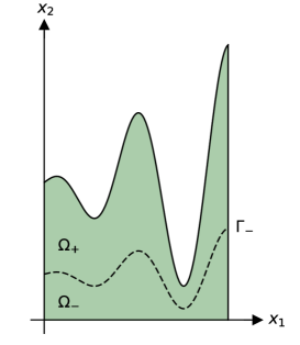
(b)

Figure 1. A locally periodic domain $\Omega^{\varepsilon}$ (a), $\varepsilon=1/8$, and the corresponding homogeneous domain $\Omega$ (b), with $\Gamma_{-}$ marked with a dashed line separating the regions $\Omega_{+}$ and $\Omega_{-}$. The particular function $\eta$ is $\eta(x,y)=(1+x\cos(4\pi x))(1+\sin(2\pi(x+y))/2)$.

The solutions $u^{\varepsilon}$ will be approximated in terms of the solution $u^{0}$ to the homogenized problem:

$$-{\mathop{\mathrm{div}}}(hA^{0}\nabla u) =hf\quad\text{ in }\Omega,$$

$$u =0\,\,\,\quad\text{ on }\Gamma,$$ (2)

$$hA^{0}\nabla u\cdot\nu =0\,\,\,\quad\text{ on }\partial\Omega\setminus\Gamma,$$

where the coefficients $A^{0}$ and the domain $\Omega$ are defined as follows. In terms of the Lipschitz functions

$$\eta_{-}(x) =\min_{y}\eta(x,y), \eta_{+}(x) =\max_{y}\eta(x,y),$$

the domain

$$\Omega =\{x\in\mathbb{R}^{2}:0<x_{1}<1,\,\,0<x_{2}<\eta_{+}(x_{1})\}$$

is separated into the regions

$$\Omega_{-} =\{x\in\mathbb{R}^{2}:0<x_{1}<1,\,\,0<x_{2}<\eta_{-}(x_{1})\},$$

$$\Omega_{+} =\{x\in\mathbb{R}^{2}:0<x_{1}<1,\,\,\eta_{-}(x_{1})<x_{2}<\eta_{+}(x_{1})\},$$

with interior interface $\Gamma_{-}=\partial\Omega_{-}\cap\partial\Omega_{+}$. The effective matrix is

$$A^{0} =\left(\begin{matrix}\chi_{\Omega_{-}}&0\\ 0&1\end{matrix}\right).$$ (3)

An illustration of $\Omega$, with the regions $\Omega_{+}$ and $\Omega_{-}$, and the interface $\Gamma_{-}$, indicated is shown in Figure 1(b), corresponding to the domain $\Omega^{\varepsilon}$ in Figure 1(a).

Let $h$ denote what we call the density of $\Omega^{\varepsilon}$ in $\Omega$:

$$Y(x) =\{y:x_{2}<\eta(x_{1},y)\},$$ (4)

$$h(x) =|Y(x)|.$$ (5)

In $\Omega_{-}$ the density is $h=1$. A part of the upper boundary, denoted by $\Gamma_{a}$ is given by

$$\Gamma_{a}=\left\{(x_{1},x_{2})\leavevmode\nobreak\ |\leavevmode\nobreak\ x_{1}\in(0,1),\leavevmode\nobreak\ x_{2}=\eta_{+}(x_{1}),\leavevmode\nobreak\ h(x_{1},x_{2})=0\right\}.$$

In order to ensure that homogenization takes place, the following hypotheses will be used:

1. $Y(x)$ is connected, $x\in\Omega$.

2. $Y(x)=k/N+Y(x)$, $x\in\Omega$, $k\in\mathbb{Z}$, for some natural number $N\geq 1$, and $Y(x)=y_{0}-Y(x)$ for some $y_{0}\in[0,1/N)$, and $Y_{0}(x)=\{y\in Y(x):y_{0}\leq y\leq y_{0}+1/(2N)\}$ is connected, $x\in\Omega$.

The hypothesis (H1) means that there is only one so-called pillar or bump in each period, and (H2) means restricting to a fundamental symmetry cell with respect to some translations and mirror symmetry. The hypothesis (H1) is stronger than (H2), and it gives a sufficient condition for homogenization. The hypothesis (H2) is included here to illustrate that it is not necessary there is only one ’bump’ in each period even if one uses the smallest periodicity cell. The graph of a function $\eta$ that satisfies (H2) but not (H1) is illustrated in Figure 3.

The assumption that $\eta$ is strictly positive ensures that the segment $\Gamma=(0,1)\times\{0\}$ is separated from the graph of $\eta(x_{1},x_{1}/\varepsilon)$, so $\Omega_{-}$ is a nonempty connected Lipschitz domain. The subdomains $\Omega_{+}$ and $\Omega_{-}$ have been chosen such that $\Omega_{+}$ covers the periodic region of $\Omega^{\varepsilon}$, and $\Omega_{+}$ is of positive measure if $\eta(x,y)$ is non-constant in $y$ for at least one $x$.

Denote by $L^{2}(\Omega,h)$ the Lebesgue space $\{v:\int_{\Omega}v^{2}h\,dx<\infty\}$, and $W(\Omega,\Gamma)$ the Sobolev space

$$W(\Omega,\Gamma) =\big{\{}v\in L^{2}(\Omega,h):A^{0}\nabla v\in L^{2}(\Omega,h),\,v=0\text{ on }\Gamma\big{\}},$$ (6)

where $A^{0}$ is defined in (3) and $h$ is defined in (4)-(5). The homogenized problem (2) has a unique solution $u^{0}\in W(\Omega,\Gamma)$.

We will first establish the homogenization of (2), that is the convergence of the solutions $u^{\varepsilon}$ and their flows $\nabla u^{\varepsilon}$ to the solution $u^{0}$ to the homogenized problem (2) and its flow $hA^{0}\nabla u^{0}$, under hypothesis that (H1) holds.

Let $u^{\varepsilon}\in H^{1}(\Omega^{\varepsilon},\Gamma)$ be the solutions to (2), and let $u^{0}\in W(\Omega,\Gamma)$ be the solution to (2). In Theorem 6.1, it is shown under hypothesis (H1) that

$$\widetilde{u^{\varepsilon}}\rightharpoonup hu^{0}\quad\text{ weakly in }L^{2}(\Omega),$$

$$\widetilde{\nabla u^{\varepsilon}}\rightharpoonup hA^{0}\nabla u^{0}\quad\text{ weakly in }L^{2}(\Omega),$$

as $\varepsilon$ tends to zero. Here tilde denotes extension by zero.

At this point we know that there will be oscillations in $\widetilde{u^{\varepsilon}}$ in the upper part $\Omega_{+}$ due to the periodicity of $\Omega_{\varepsilon}$, while no oscillations in the lower part $\Omega_{-}$ due to the compact embedding of $H^{1}(\Omega_{-})$ into $L^{2}(\Omega_{-})$. Moreover, we cannot at this point exclude the possibility of oscillations in the solutions $\widetilde{u^{\varepsilon}}$ due to something else, as the above weak convergences may be expressed as weak unfolding or two-scale convergence. A next step is to check whether the strong unfolding convergence holds for the solutions $u^{\varepsilon}$ and their flows.

The weak convergence of the zero extensions in the upper part $\Omega_{+}$ cannot be strong, unless the limit is zero. To this end we first describe the error measured in the oscillating domain. Not only are the unfoldings of the solutions $u^{\varepsilon}$ and their flows strongly converging, there are no oscillations.

For $u^{\varepsilon}$ the solutions to (2) and $u^{0}$ the solution to (2), in Theorem 7.1 it is shown under hypothesis (H1) that

$$\|u^{\varepsilon}-u^{0}\|_{L^{2}(\Omega^{\varepsilon},\,h)}\to 0,$$

$$\|\nabla u^{\varepsilon}-A^{0}\nabla u^{0}\|_{L^{2}(\Omega^{\varepsilon},\,h)}\to 0,$$

as $\varepsilon$ tends to zero.

Turning back to the question of homogenization, there is an extension of the solutions $u^{\varepsilon}$ and their flows for which strong convergence holds in $L^{2}(\Omega)$.

For $u^{\varepsilon}$ the solutions to (2) and $u^{0}$ the solution to (2), in Theorem 8.1 it is shown that when the functions are extended in a way preserving their average, under hypothesis (H1) (c.f. [38, 26]),

$$\widetilde{u^{\varepsilon}}^{m}\to u^{0}\quad\text{ strongly in }L^{2}(\Omega,h),$$

$$\widetilde{\nabla u^{\varepsilon}}^{m}\to A^{0}\nabla u^{0}\quad\text{ strongly in }L^{2}(\Omega,h),$$

as $\varepsilon$ tends to zero, when $\sim{\!m}$ denotes the particular extension ((25), (26) in Section 8). It is remarked that the above mentioned convergences also hold under hypothesis (H2).

Without the hypotheses (H1), (H2), under a slightly milder restriction on the domain, in Theorem 10.1 it is shown that the solutions $u^{\varepsilon}$ to (2) converge to the solution $u^{0}$ to the limit problem (10), with $A^{0}$ given by (29), in the sense that

$$\widetilde{u^{\varepsilon}} \rightharpoonup\int_{Y(x)}u^{0}\,dy\quad\text{ weakly in }L^{2}(\Omega),$$

$$\widetilde{\nabla u^{\varepsilon}} \rightharpoonup\int_{Y(x)}A^{0}\nabla_{x}u^{0}\,dy\quad\text{ weakly in }L^{2}(\Omega),$$

as $\varepsilon$ tends to zero. One also has strong unfolding convergence. We do not analyze further the convergence in the case of non-connected sections.

In the case of the homogeneous Dirichlet condition on the oscillating part of the boundary, the limit is trivial in the oscillating part. This case was studied in [5].

Remark 2.1 (The effect of anisotropy and oscillating coefficients).

To illustrate the effect of anisotropy and oscillating coefficients on the asymptotic behavior of the solutions $u^{\varepsilon}$ to (2), one can consider the following elliptic model problem:

$$-{\mathop{\mathrm{div}}}\big{(}A\big{(}x,\frac{x_{1}}{\varepsilon}\big{)}\nabla u\big{)} =f\quad\text{ in }\Omega^{\varepsilon},$$

$$u =0\quad\text{ on }\Gamma,$$

$$A\big{(}x,\frac{x_{1}}{\varepsilon}\big{)}\nabla u\cdot\nu =0\quad\text{ on }\partial\Omega^{\varepsilon}\setminus\Gamma,$$

under the assumption that the not necessarily symmetric matrix $A\in C^{1}(\overline{\Omega},L^{\infty}(\mathbb{T}))$ satisfies the ellipticity condition

$$A(x,y)\xi\cdot\xi\geq C|\xi|^{2},\quad x\in\Omega,\,y\in\mathbb{T},\,\xi\in\mathbb{R}^{2}.$$

Suppose further that hypothesis (H2) is satisfied, and that the coefficient matrix satisfies the corresponding symmetry conditions: $A(x,y)=A(x,k/N+y)$, $k\in\mathbb{Z}$, and $A(x,y)=A(x,y_{0}-y)$, for $x\in\Omega_{+}$, where $N$ and $y_{0}$ are the same as for $Y(x)$ in (H2). Then the weak limits of $\widetilde{u^{\varepsilon}}$ and $\widetilde{\nabla u^{\varepsilon}}$ are $hu^{0}$ and $A^{0}u^{0}$, respectively, in $L^{2}(\Omega)$, as $\varepsilon$ tends to zero, where $u^{0}$ solves the limit problem

$$-{\mathop{\mathrm{div}}}(A^{0}\nabla u) =hf\quad\text{ in }\Omega,$$

$$u =0\,\,\,\quad\text{ on }\Gamma,$$

$$A^{0}\nabla u\cdot\nu =0\,\,\,\quad\text{ on }\partial\Omega\setminus\Gamma,$$

where the entries $A^{0}_{ij}$ of the effective matrix $A^{0}$ are given by, here including $h$,

$$A^{0}_{11} =\chi_{\Omega_{-}}\Big{(}\int_{Y(x)}\frac{1}{A_{11}}\,dy\Big{)}^{-1},$$

$$A^{0}_{12} =A^{0}_{11}\int_{Y(x)}\frac{A_{12}}{A_{11}}\,dy,$$

$$A^{0}_{21} =A^{0}_{11}\int_{Y(x)}\frac{A_{21}}{A_{11}}\,dy,$$

$$A^{0}_{22} =A^{0}_{11}\int_{Y(x)}\frac{A_{12}}{A_{11}}\,dy\int_{Y(x)}\frac{A_{21}}{A_{11}}\,dy+\int_{Y(x)}\frac{{\mathop{\mathrm{det}}}A}{A_{11}}\,dy,$$

where $A_{ij}$ denote the entries of the local matrix $A$. In the fixed region $\Omega_{-}$, $A^{0}$ is the classical effective matrix for layered materials because there $Y(x)=\mathbb{T}$, while in the oscillating region $\Omega_{+}$ all but the last term in $A_{22}^{0}$ vanish due to the insulation in the $x_{1}$ direction. In particular, for $-\Delta$ the effective matrix reduces to the matrix given in (3). A similar statement can be made for the case of non-connected sections analogous to Theorem 10.1.

3. Asymptotic expansions for the solutions

To derive the homogenized equation (2) for the solutions $u^{\varepsilon}$ to the equation

$$-\Delta u^{\varepsilon} =f\quad\text{ in }\Omega^{\varepsilon},$$ (7)

asymptotic expansions may be used, in the form of a formal power series in the small parameter $\varepsilon$. In the problem (7), in the periodic region $\Omega^{\varepsilon}_{+}$ of the domain $\Omega$, $\varepsilon$ represents both the periodicity in the $x_{1}$ direction, as well as the order of magnitude of the widths of the pillars with homogeneous Neumann condition on their sides. In the fixed region $\Omega_{-}$ of the domain, $\varepsilon$ represents the periodicity on the interface $\Gamma_{-}$.

The above reasoning leads us to consider the following Bakhvalov ansatz for inner expansion in the periodic region $\Omega^{\varepsilon}_{+}$:

$$u^{\varepsilon}(x)\sim\big{(}u^{0}_{+}(x_{2},y)+\varepsilon u^{1}_{+}(x_{2},y)+\varepsilon^{2}u^{2}_{+}(x_{2},y)\big{)}\Big{|}_{\displaystyle y=\frac{x_{1}}{\varepsilon}},$$ (8)

where $u^{i}_{+}$ are assumed to be periodic in $y$.

Let $\chi(x,y)$ denote the characteristic function of the set

$$\{(x,y):0<x_{1}<1,\,\,0<x_{2}<\eta(x_{1},y)\}.$$

Then the characteristic function of $\Omega^{\varepsilon}$ is

$$\chi_{\Omega^{\varepsilon}}(x)=\chi\big{(}x,\frac{x_{1}}{\varepsilon}\big{)}.$$

We write (7) in the homogeneous domain $\Omega$ as follows:

$$-\sum_{i}\frac{\partial}{\partial x_{i}}\big{(}\chi\big{(}x,\frac{x_{1}}{\varepsilon}\big{)}\frac{\partial}{\partial x_{i}}u^{\varepsilon}\big{)} =\chi\big{(}x,\frac{x_{1}}{\varepsilon}\big{)}f\quad\text{ in }\Omega.$$ (9)

With the ansatz (8),

$$\Delta\sim\frac{1}{\varepsilon^{2}}\frac{\partial^{2}}{\partial y^{2}}+\frac{\partial^{2}}{\partial x_{2}^{2}}.$$

A substitution of (8) into (9) and collecting similar powers of $\varepsilon$ result in the following equations for the initial powers of $\varepsilon$:

$$\varepsilon^{-2}:\quad -\frac{\partial}{\partial y}\big{(}\chi\frac{\partial u^{0}_{+}}{\partial y}\big{)}=0,$$

$$\varepsilon^{-1}:\quad -\frac{\partial}{\partial y}\big{(}\chi\frac{\partial u^{1}_{+}}{\partial y}\big{)}=0,$$

$$\varepsilon^{0}:\quad -\frac{\partial}{\partial y}\big{(}\chi\frac{\partial u^{2}_{+}}{\partial y}\big{)}=\frac{\partial}{\partial x_{2}}\big{(}\chi\frac{\partial u^{0}_{+}}{\partial x_{2}}\big{)}+\chi f.$$

The equation for power $\varepsilon^{-2}$ suggests that $u^{0}_{+}$ is independent of $y$, under the assumption that $Y(x)$ is connected, or some discrete symmetry in the problem such as (H2). Viewing the above equations as definitions of $u^{i}_{+}$ in $\mathbb{T}$ with $x$ as a parameter, the compatibility condition for $u^{2}_{+}$ may be read off from the $\varepsilon^{0}$ equation:

$$\int_{\mathbb{T}}\big{(}\frac{\partial}{\partial x_{2}}\big{(}\chi\frac{\partial u^{0}_{+}}{\partial x_{2}}\big{)}+\chi f\big{)}\,dy =0.$$

Because

$$\int_{\mathbb{T}}\chi(x,y)\,dy =\int_{Y(x)}dy=|Y(x)|=h(x),$$

where

$$Y(x) =\{y:x_{2}<\eta(x_{1},y)\},$$

$$h(x) =|Y(x)|,$$

the compatibility condition is

$$-\frac{\partial}{\partial x_{2}}\big{(}h\frac{\partial u^{0}_{+}}{\partial x_{2}}\big{)} =hf\quad\text{ in }\Omega_{+}.$$ (10)

The equation (10) is the homogenized equation for $u^{\varepsilon}$ in the periodic part $\Omega_{+}$ of $\Omega$.

In the fixed region $\Omega_{-}$ of the domain, the equation (7) reads

$$-\Delta u^{\varepsilon} =f\quad\text{ in }\Omega_{-}.$$ (11)

Consider the following ansatz for inner expansion in the fixed region $\Omega_{-}$:

$$u^{\varepsilon}(x)\sim\big{(}u^{0}_{-}(x,y)+\varepsilon u^{1}_{-}(x,y)+\varepsilon^{2}u^{2}_{-}(x,y)\big{)}\Big{|}_{\displaystyle y=\frac{x_{1}}{\varepsilon}},$$ (12)

where $u^{i}_{-}$ are assumed to be periodic in $y$. With the ansatz (12),

$$\Delta\sim\frac{1}{\varepsilon^{2}}\frac{\partial^{2}}{\partial y^{2}}+\frac{2}{\varepsilon}\frac{\partial^{2}}{\partial y\partial x_{1}}+\Delta_{x}.$$

A substitution of (12) into (11) and collecting similar powers of $\varepsilon$ result in the following equations for the initial powers of $\varepsilon$:

$$\varepsilon^{-2}:\quad -\frac{\partial^{2}u^{0}_{-}}{\partial y^{2}}=0,$$

$$\varepsilon^{-1}:\quad -\frac{\partial^{2}u^{1}_{-}}{\partial y^{2}}=2\frac{\partial^{2}u^{0}_{-}}{\partial y\partial x_{1}},$$

$$\varepsilon^{0}:\quad -\frac{\partial^{2}u^{2}_{-}}{\partial y^{2}}=2\frac{\partial^{2}u^{1}_{-}}{\partial y\partial x_{1}}+\Delta_{x}u^{0}_{-}+f.$$

The equation for power $\varepsilon^{-2}$ suggests that $u^{0}_{-}$ is independent of $y$. By the periodicity of $u^{1}_{-}$, the compatibility condition for $u^{2}_{-}$ reads

$$-\Delta u^{0}_{-} =f\quad\text{ in }\Omega_{-}.$$

In order $u^{0}=\chi_{\Omega_{-}}u^{0}_{-}+\chi_{\Omega_{+}}u^{0}_{+}$ to be globally defined, an interface condition is needed on $\Gamma_{-}=\partial\Omega_{-}\cap\partial\Omega_{+}$. If one requires continuity of $u^{0}$ and its flow on $\Gamma_{-}$, one must have $u^{0}_{+}=u^{0}_{-}$ on $\Gamma_{-}$, as well as

$$\Big{(}\begin{matrix}1&0\\ 0&h\end{matrix}\Big{)}\nabla u^{0}_{+}\cdot\nu-\nabla u^{0}_{-}\cdot\nu=0,$$

where $\nu$ is one of the unit normals on $\Gamma_{-}$, and the upper left entry of the matrix in the first term is arbitrary. This condition becomes explicitly,

$$h\frac{\partial u^{0}_{+}}{\partial x_{2}}\nu_{2}-\nabla u^{0}_{-}\cdot\nu=0,$$

which may be expressed as

$$[hA^{0}\nabla u^{0}\cdot\nu]=0\quad\text{ on }\Gamma_{-},$$

where $[\cdot]$ denotes the jump on $\Gamma_{-}$, and $A^{0}$ is given by (3).

4. Example of behavior of the solutions in a degenerating case

The solution $u^{0}$ to the homogenized problem (2) may belong to $H^{1}(\Omega)$ even if $h(x)$ tends to zero as $x$ approaches $M=\{x:h(x)=0\}\subset\partial\Omega$, as the following example illustrates. Consider the case $f=1$ with $\eta(x,y)=\hat{\eta}(y)$ the piecewise linear function given by $\hat{\eta}(0)=1$ and $\hat{\eta}(1/2)=2$, that is $\hat{\eta}(y)=2-2|y-1/2|$. The homogeneous domains are $\Omega=(0,1)\times(0,2)$, $\Omega_{+}=(0,1)\times(1,2)$, $\Omega_{-}=(0,1)\times(0,1)$, and the interface is $\Gamma_{-}=(0,1)\times\{1\}$. In Figure 2, illustrations of the domains $\Omega^{\varepsilon}$ and $\Omega$ are shown. In this case,

$$h(x) =\begin{cases}2-x_{2}&\text{ in }\Omega_{+},\\ 1&\text{ in }\overline{\Omega_{-}},\end{cases}$$

and

$$h =0\quad\text{ on }M=\{x:h(x)=0\}=(0,1)\times\{2\},$$

$$h =1\quad\text{ on }\Gamma_{-}.$$

The solution to the homogenized problem (2) is

$$u^{0}(x) =\begin{cases}1/4+x_{2}-x_{2}^{2}/4&\text{ in }\Omega_{+},\\ 3x_{2}/2-x_{2}^{2}/2&\text{ in }\overline{\Omega_{-}}.\end{cases}$$

In particular, $u^{0}\in H^{1}(\Omega)$ and it has continuous gradient over the interface $\Gamma_{-}$.

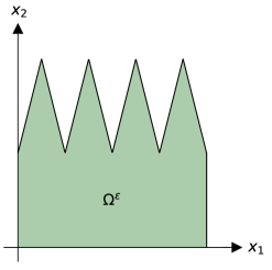
(a)

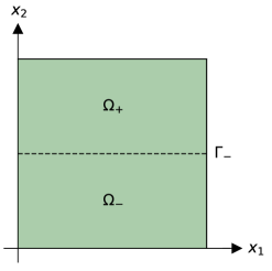
(b)

Figure 2. A locally periodic domain $\Omega^{\varepsilon}$ (a), $\varepsilon=1/4$, and the corresponding homogeneous domain $\Omega$ (b), with interface $\Gamma_{-}$ marked as a dashed line separating the regions $\Omega_{+}$ and $\Omega_{-}$.

5. Periodic unfolding

The only apparent possible cause of oscillations in the solutions to (2) and their flows is the periodicity in the domain, in the $x_{1}$ direction. For the study of these oscillations we will use periodic unfolding.

The periodic unfolding at rate $\varepsilon$ of a function $v:\mathbb{R}^{2}\to\mathbb{R}$ along $x_{1}$ is

$$(T^{\varepsilon}v)(x,y) =v\big{(}\varepsilon\big{[}\frac{x_{1}}{\varepsilon}\big{]}+\varepsilon y,x_{2}\big{)},$$

where $[\cdot]$ denotes the integer part, and $v$ is extended by zero when necessary. Using this change of variables for the periodic coefficient $\chi_{\Omega^{\varepsilon}_{+}}$ in (2), the characteristic function of the region of $\Omega^{\varepsilon}$ where coefficients are periodic,

$$\Omega^{\varepsilon}_{+} =\big{\{}x\in\mathbb{R}^{2}:0<x_{1}<1,\,\,\eta_{-}(x_{1})<x_{2}<\eta\big{(}x_{1},\frac{x_{1}}{\varepsilon}\big{)}\big{\}},$$

gives $\chi_{\Omega^{\varepsilon}_{u}}$, the characteristic function of the domain

$$\Omega^{\varepsilon}_{u} =\big{\{}(x,y)\in\mathbb{R}^{2}\times\mathbb{T}:0<x_{1}<1,\,\,\eta_{-}\big{(}\varepsilon\big{[}\frac{x_{1}}{\varepsilon}\big{]}+\varepsilon y\big{)}<x_{2}<\eta\big{(}\varepsilon\big{[}\frac{x_{1}}{\varepsilon}\big{]}+\varepsilon y,y\big{)}\big{\}}.$$

There holds

$$T^{\varepsilon}\chi_{\Omega^{\varepsilon}_{+}} =\chi_{\Omega^{\varepsilon}_{u}}\to\chi_{\Omega_{u}}\quad\text{ strongly in }L^{p}(\mathbb{R}^{2}\times\mathbb{T}),\quad 1\leq p<\infty,$$ (13)

where

$$\Omega_{u} =\{(x,y)\in\mathbb{R}^{2}\times\mathbb{T}:0<x_{1}<1,\,\,\eta_{-}(x_{1})<x_{2}<\eta(x_{1},y)\}$$

$$=\{(x,y)\in\mathbb{R}^{2}\times\mathbb{T}:x\in\Omega_{+},\,\,y\in Y(x)\}.$$

The property (13) is the strong unfolding convergence of the sequence and it will be used in the passage from periodic domain to a fixed domain in integrals. It expresses that $\chi_{\Omega_{+}^{\varepsilon}}$ converges weakly in $L^{p}(\mathbb{R}^{2})$ while not strongly, and that the oscillation spectrum of the sequence belongs to the integers if not empty. To obtain (13) one uses the almost everywhere pointwise convergence of $\chi_{\Omega^{\varepsilon}_{u}}$ to $\chi_{\Omega_{u}}$ and the Lebesgue dominated convergence theorem, or views it as a consequence of Lemma 5.1 below.

The cost of replacing in integrals the $\varepsilon$ depending unfolded domain $\Omega^{\varepsilon}_{u}$ with the fixed domain $\Omega_{u}$ is described by the following lemma.

Lemma 5.1.

Let $\Omega$ contain $\Omega^{\varepsilon}_{+}$. Suppose that $\|v^{\varepsilon}\|_{L^{p}(\Omega)}\leq C$ and $p>1$. Then

$$\int_{\Omega^{\varepsilon}_{+}}v^{\varepsilon}\,dx =\int_{\Omega_{u}}T^{\varepsilon}v^{\varepsilon}\,dxdy+O(\varepsilon^{1-1/p}),$$

as $\varepsilon$ tends to zero.

Proof.

Because $T^{\varepsilon}\chi_{\Omega_{+}^{\varepsilon}}=\chi_{\Omega_{u}^{\varepsilon}}$, the discrepancy can be computed as follows:

$$\int_{\Omega_{+}^{\varepsilon}}v^{\varepsilon}\,dx-\int_{\Omega_{u}}T^{\varepsilon}v^{\varepsilon}\,dxdy =\int_{\Omega\times\mathbb{T}}T^{\varepsilon}\chi_{\Omega_{+}^{\varepsilon}}T^{\varepsilon}v^{\varepsilon}\,dxdy-\int_{\Omega_{u}}T^{\varepsilon}v^{\varepsilon}\,dxdy$$

$$=\int_{\Omega\times\mathbb{T}}(\chi_{\Omega^{\varepsilon}_{u}}-\chi_{\Omega_{u}})T^{\varepsilon}v^{\varepsilon}\,dxdy.$$

The differences $\Omega_{u}^{\varepsilon}\setminus\Omega_{u}$ and $\Omega_{u}\setminus\Omega_{u}^{\varepsilon}$ are contained in some strip of measure $O(\varepsilon)$:

$$\{(x,y)\in\mathbb{R}^{2}\times\mathbb{T}:\mathrm{dist}((x,y),\partial\Omega_{u})<C\varepsilon\},$$

where $C$ may be chosen independent of $\varepsilon$ by the Lipschitz continuity of $\eta$ and $\eta_{-}$,

By the Hölder inequality,

$$\Big{|}\int_{\Omega^{\varepsilon}_{+}}v^{\varepsilon}\,dx-\int_{\Omega_{u}}T^{\varepsilon}v^{\varepsilon}\,dxdy\Big{|} \leq\|\chi_{\Omega_{u}^{\varepsilon}}-\chi_{\Omega_{u}}\|_{L^{1/(1-1/p)}(\Omega\times\mathbb{T})}\|v^{\varepsilon}\|_{L^{p}(\Omega)}=O(\varepsilon^{(p-1)/p}),$$

which gives the desired estimate. ∎

6. Homogenization

In this section we establish the homogenization of problem (2) to (2) in the sense of weak convergence of the solutions and their flows. The method we use is the unfolding Lemma 5.1 to pass to the fixed domain $\Omega_{u}$, and the weak compactness in $L^{2}(\Omega_{u})$ to characterize the asymptotic behavior of $u^{\varepsilon}$.

Throughout this section (H1) is assumed to hold.

Theorem 6.1.

Suppose that (H1) holds. Let $u^{\varepsilon}\in H^{1}(\Omega^{\varepsilon},\Gamma)$ be the solutions to (2), and let $u^{0}\in W(\Omega,\Gamma)$ be the solution to (2). Then

$$\emph{(i)}\quad\widetilde{u^{\varepsilon}}\rightharpoonup hu^{0}\quad\text{ weakly in }L^{2}(\Omega),$$

$$\emph{(ii)}\quad\widetilde{\nabla u^{\varepsilon}}\rightharpoonup hA^{0}\nabla u^{0}\quad\text{ weakly in }L^{2}(\Omega),$$

as $\varepsilon$ tends to zero, where $\sim$ denotes extension by zero.

The convergence of the flows in Theorem 6.1(ii) means that $u^{\varepsilon}$ converges weakly to $u^{0}$ in $H^{1}(\Omega_{-},\Gamma)$, and strongly in $L^{2}(\Omega_{-})$ by the Relich theorem.

Lemma 6.1.

For any $\varepsilon=1/k$, $k=1,2,\ldots$, there exists a unique solution $u^{\varepsilon}\in H^{1}(\Omega^{\varepsilon},\Gamma)$ to (2). For the solutions $u^{\varepsilon}$, the following a priori estimate holds:

$$\|u^{\varepsilon}\|_{H^{1}(\Omega^{\varepsilon},\,\Gamma)}\leq C,$$

where $C$ is independent of $\varepsilon$.

Proof.

The variational form of (2) is: Find $u^{\varepsilon}\in H^{1}(\Omega^{\varepsilon},\Gamma)$ such that

$$\int_{\Omega^{\varepsilon}}\nabla u\cdot\nabla\psi\,dx =\int_{\Omega^{\varepsilon}}f\psi\,dx,$$ (14)

for all $\psi\in H^{1}(\Omega^{\varepsilon},\Gamma)$. Using the Poincaré inequality

$$\int_{\Omega^{\varepsilon}}v^{2}\,dx\leq(\max\eta_{+})^{2}\int_{\Omega^{\varepsilon}}\Big{(}\frac{\partial v}{\partial x_{2}}\Big{)}^{2}\,dx,\quad v\in H^{1}(\Omega^{\varepsilon},\Gamma),$$

one verifies that left hand side in (14) is an inner product on $H^{1}(\Omega^{\varepsilon},\Gamma)$. The right hand side in (14) is a bounded linear functional on $H^{1}(\Omega^{\varepsilon},\Gamma)$. The Riesz theorem guarantees the existence of a unique solution $u^{\varepsilon}\in H^{1}(\Omega^{\varepsilon},\Gamma)$. Using $u^{\varepsilon}$ as a test function in (14) gives

$$\|u^{\varepsilon}\|_{H^{1}(\Omega^{\varepsilon},\,\Gamma)} \leq C\|f\|_{L^{2}(\Omega)},$$

uniformly in $\varepsilon$ by the uniform Poincaré constant, from which the desired a priori estimate is obtained. ∎

Lemma 6.2.

For the sequence of solutions $u^{\varepsilon}$ to (2), the following a priori estimates hold for the unfolded sequences:

$$\|T^{\varepsilon}u^{\varepsilon}\|_{L^{2}(\Omega_{u})} \leq C,$$

$$\|T^{\varepsilon}\nabla u^{\varepsilon}\|_{L^{2}(\Omega_{u})} \leq C,$$

where $C$ is independent of $\varepsilon$.

Proof.

By the definition of unfolding,

$$\int_{\Omega^{\varepsilon}_{+}}(u^{\varepsilon})^{2}\,dx =\int_{\Omega_{u}^{\varepsilon}}(T^{\varepsilon}u^{\varepsilon})^{2}\,dxdy=\int_{\Omega_{u}}(T^{\varepsilon}u^{\varepsilon})^{2}\,dxdy+\int_{\Omega_{u}^{\varepsilon}\setminus\Omega_{u}}(T^{\varepsilon}u^{\varepsilon})^{2}\,dxdy,$$

because $T^{\varepsilon}u^{\varepsilon}$ is zero outside $\Omega_{u}^{\varepsilon}$. By using the estimate for the solutions $u^{\varepsilon}$ in Lemma 6.1, the estimate $\|T^{\varepsilon}u^{\varepsilon}\|_{L^{2}(\Omega_{u})}\leq C$ is obtained. The same computation with $|\nabla u^{\varepsilon}|$ in place of $u^{\varepsilon}$ gives the estimate $\|T^{\varepsilon}\nabla u^{\varepsilon}\|_{L^{2}(\Omega_{u})}\leq C$. ∎

Regarding the function space, $W(\Omega,\Gamma)$ is associated to the homogenized problem (2). In the cover $\Omega_{+}$ of the periodic region of $\Omega^{\varepsilon}$, the $H^{1}(\Omega)$ ellipticity of the operator to the homogenized problem (2) may be violated. For

$$hA^{0}\xi\cdot\xi =\begin{cases}h\xi_{2}^{2}\quad\text{ in }\overline{\Omega_{+}},\\ |\xi|^{2}\quad\text{ in }\Omega_{-},\end{cases}$$

and $h(x)$ tends to zero as $x$ approaches $M=\{x:h(x)=0\}$, which might be nonempty. The properties

$$h(x)>0\quad\text{in }\Omega,$$

$$h,h^{-1}\in L^{1}_{\mathrm{loc}}(\Omega),$$

ensure that $W(\Omega,\Gamma)$ is a Hilbert space when equipped with the inner product $(u,v)=\int_{\Omega}A^{0}\nabla u\cdot\nabla v\,dx$, and that $C^{\infty}_{0}(\Omega)$ is embedded into $W(\Omega,\Gamma)$. We denote by $C^{\infty}(\Omega,\Gamma)$, the $C^{\infty}(\Omega)$ functions vanishing in a neighborhood of $\Gamma$.

The existence of a solution $u^{0}\in W(\Omega,\Gamma)$ to $\eqref{eq:limitproblem}$ is obtained by weak compactness in the proof of Theorem 6.1 below, with uniqueness by linearity. One might also obtain it in the direct way as follows.

Lemma 6.3.

There exists a unique solution $u^{0}\in W(\Omega,\Gamma)$ to $\eqref{eq:limitproblem}$.

Proof.

The variational form of (2) is: Find $u^{0}\in W(\Omega,\Gamma)$ such that

$$\int_{\Omega}hA^{0}\nabla u^{0}\cdot\nabla\psi\,dx =\int_{\Omega}f\psi h\,dx,$$ (15)

for all $\psi\in W(\Omega,\Gamma)$.

The Hilbert space structure on $W(\Omega,\Gamma)$ has been chosen such that

$$\int_{\Omega}hA^{0}\nabla v\cdot\nabla v\,dx =\|v\|_{W(\Omega,\,\Gamma)}^{2}.$$

By the Hölder and Poincaré inequalities, the left hand side of (15) defines an inner product on $W(\Omega,\Gamma)$. The right hand side of (15) is a bounded linear functional on $W(\Omega,\Gamma)$. By the Riesz theorem, there exists a unique $u^{0}\in W(\Omega,\Gamma)$ satisfying (15). ∎

Proof of Theorem 6.1.

From Lemma 6.1 and Lemma 6.2 we have the following a priori estimates for the solutions $u^{\varepsilon}$ to problem (2) and their unfoldings:

$$\|u^{\varepsilon}\|_{H^{1}(\Omega^{\varepsilon},\,\Gamma)} \leq C,$$

$$\|T^{\varepsilon}u^{\varepsilon}\|_{L^{2}(\Omega_{u})} \leq C,$$

$$\|T^{\varepsilon}\nabla u^{\varepsilon}\|_{L^{2}(\Omega_{u})} \leq C.$$

By weak compactness, there exist $u^{0}_{-}\in H^{1}(\Omega_{-},\Gamma)$, $u^{0}_{+}\in L^{2}(\Omega_{u})$, $p\in L^{2}(\Omega_{u})$, and a subsequence of $\varepsilon$ which we still denoted by $\varepsilon$, such that

$$u^{\varepsilon} \rightharpoonup u^{0}_{-}\quad\qquad\quad\text{ weakly in }H^{1}(\Omega_{-},\,\Gamma),$$ (16)

$$T^{\varepsilon}u^{\varepsilon} \rightharpoonup u^{0}_{+}\quad\qquad\quad\text{ weakly in }L^{2}(\Omega_{u}),$$ (17)

$$T^{\varepsilon}\nabla u^{\varepsilon} \rightharpoonup\big{(}p,\frac{\partial u^{0}_{+}}{\partial x_{2}}\big{)}\,\,\quad\text{ weakly in }L^{2}(\Omega_{u}),$$ (18)

where the equality of second component of the weak limit of $T^{\varepsilon}\nabla u^{\varepsilon}$ and $\frac{\partial u^{0}_{+}}{\partial x_{2}}$, and that $u^{0}_{+}$ does not depend on $y$, follow from the boundedness of the sequences and

$$\frac{\partial}{\partial x_{2}}T^{\varepsilon}u^{\varepsilon} =T^{\varepsilon}\frac{\partial u^{\varepsilon}}{\partial x_{2}}, \frac{\partial}{\partial y}T^{\varepsilon}u^{\varepsilon} =\varepsilon T^{\varepsilon}\frac{\partial u^{\varepsilon}}{\partial x_{1}}.$$ (19)

By (H1) and (19), $u^{0}_{+}$ does not depend on $y$.

Claim 1: The average of $p$ in $y$ is zero: $\int_{Y(x)}p\,dy=0$, a.e. $x\in\Omega_{+}$.

Information about $p$ may be obtained by using oscillating test functions in the equation for $u^{\varepsilon}$ (c.f. [40, 54]). The prototype $\varphi^{\varepsilon}=\varepsilon\phi(x)\{x_{1}/\varepsilon\}$, with $\phi\in C^{\infty}_{0}(\Omega_{+})$ and $\{\cdot\}$ denoting fractional part, would serve the purpose in view of (22) because $T^{\varepsilon}\varphi^{\varepsilon}\to 0$ and $T^{\varepsilon}\nabla\varphi^{\varepsilon}\to(\phi,0)$ strongly in $L^{2}(\Omega_{u})$. As $\varphi^{\varepsilon}$ are not necessarily continuous on $\Omega^{\varepsilon}_{+}$, appropriate shifts are introduced as follows. Note that

$$\varepsilon\big{\{}\frac{x_{1}}{\varepsilon}\big{\}}=x_{1}-x_{k}^{\varepsilon},\quad\text{ if }x_{1}\in[x_{k}^{\varepsilon},x_{k+1}^{\varepsilon})\text{ and }x^{\varepsilon}_{k}=k\varepsilon.$$

Replace $x^{\varepsilon}_{k}=k\varepsilon$ with a grid where the graphs of $\eta(x_{1},x_{1}/\varepsilon)$ and $\eta_{-}(x_{1})$ are close:

$$x^{\varepsilon}_{k} \in\operatorname*{arg\,min}_{x\in\varepsilon[k,k+1]}\eta\big{(}x,\frac{x}{\varepsilon}\big{)},\quad k=0,\ldots,\frac{1}{\varepsilon}-1.$$ (20)

Let $\phi\in C^{\infty}_{0}(\Omega_{+})$. Then with $x_{k}^{\varepsilon}$ as in (20),

$$\varphi^{\varepsilon}(x) =(x_{1}-x_{k}^{\varepsilon})\phi(x),\quad\text{ if }x_{1}\in[x_{k}^{\varepsilon},x^{\varepsilon}_{k+1}),$$ (21)

belongs to $C^{\infty}(\Omega_{+}^{\varepsilon})$ for all small enough $\varepsilon$. Indeed,

$$\eta\big{(}x_{k}^{\varepsilon},\frac{x_{k}^{\varepsilon}}{\varepsilon}\big{)}-\eta_{-}(x_{k}^{\varepsilon})$$

$$\quad=\min_{x\in\varepsilon[k,k+1]}\eta\big{(}x,\frac{x}{\varepsilon}\big{)}-\min_{y}\eta(x_{k}^{\varepsilon},y)$$

$$\quad\leq\max_{\xi\in\varepsilon[k,k+1]}\big{(}\!\min_{y}\eta(\xi,y)-\min_{y}\eta(x_{k}^{\varepsilon},y)\big{)}$$

$$\quad\leq C\varepsilon,$$

by the Lipschitz continuity of $\eta_{-}$, and $\phi$ is compactly supported.

With $\varphi^{\varepsilon}$ given by (20), (21) as test functions in the equation (22) for $u^{\varepsilon}$, and using that

$$T^{\varepsilon}\varphi^{\varepsilon} \to 0,$$

$$T^{\varepsilon}\nabla\varphi^{\varepsilon} \to(\phi,0),$$

strongly in $L^{2}(\Omega_{u})$ as $\varepsilon$ tends to zero because $|x_{1}-x_{k}^{\varepsilon}|\leq\varepsilon$, one obtains in the limit

$$\int_{\Omega_{u}}p\phi\,dxdy=\int_{\Omega_{+}}\,\int_{Y(x)}p\,dy\,\phi\,dx=0,\quad\phi\in C^{\infty}_{0}(\Omega_{+}).$$

which gives the first claim.

Claim 2: $\chi_{\Omega_{-}}u^{0}_{-}+\chi_{\Omega_{+}}u^{0}_{+}\in W(\Omega,\Gamma)$ and is the solution to the homogenized problem (2).

To verify that $\chi_{\Omega_{-}}u^{0}_{-}+\chi_{\Omega_{+}}u^{0}_{+}\in W(\Omega,\Gamma)$ it suffices to check that $u^{0}_{-}=u^{0}_{+}$ in $L^{2}(\Gamma_{-})$. Note that $u^{0}_{+}\in L^{2}(\Omega_{u})$ is continuously traced into $L^{2}(\Gamma_{-})$ because $h>0$ in a neighborhood of $\Gamma_{-}$ in $\Omega$ (see Remark 6.1).

Because $u^{\varepsilon}\rightharpoonup u^{0}_{-}$ weakly in $H^{1}(\Omega_{-})$, the weak continuity of the trace gives $u^{\varepsilon}\rightharpoonup u^{0}_{-}$ weakly in $L^{2}(\Gamma_{-})$, and so $T^{\varepsilon}u^{\varepsilon}(x_{1},\eta_{-}(x_{1}))\rightharpoonup u^{0}_{-}(x_{1},\eta_{-}(x_{1}))$ weakly in $L^{2}((0,1)\times\mathbb{T})$, as $\varepsilon$ tends to zero. Denote $\Gamma_{\varepsilon}=\Omega_{\varepsilon}\cap\Gamma_{-}$. Let $\phi\in C^{\infty}_{0}(\Omega)$. On the one hand,

$$\int_{\Gamma_{\varepsilon}}u^{\varepsilon}\phi\nu_{2}\,d\sigma =\int_{0}^{1}(\chi_{\Gamma_{\varepsilon}}u^{\varepsilon}\phi\nu_{2})(x_{1},\eta_{-}(x_{1}))\,dx_{1}$$

$$=\int_{0}^{1}\int_{\mathbb{T}}T^{\varepsilon}(\chi_{\Gamma_{\varepsilon}}u^{\varepsilon}\phi\nu_{2})(x_{1},\eta_{-}(x_{1}))\,dy\,dx_{1}$$

$$\to\int_{0}^{1}\int_{\mathbb{T}}(\chi_{Y(x)}u^{0}_{-}\phi\nu_{2})(x_{1},\eta_{-}(x_{1}))\,dy\,dx_{1}$$

$$=\int_{\Gamma_{-}}hu^{0}_{-}\phi\nu_{2}\,d\sigma,$$

as $\varepsilon$ tends to zero, because $T^{\varepsilon}\chi_{\Gamma_{\varepsilon}}(x_{1},\eta_{-}(x_{1}))$ converges to $\chi_{Y(x_{1},\eta_{-}(x_{1}))}(y)$ strongly in $L^{2}((0,1)\times\mathbb{T})$. On the other hand,

$$\int_{\Gamma_{\varepsilon}}u^{\varepsilon}\phi\nu_{2}\,d\sigma =\int_{\Omega_{u}}T^{\varepsilon}\frac{\partial u^{\varepsilon}}{\partial x_{2}}T^{\varepsilon}\phi\,dxdy+\int_{\Omega_{u}}T^{\varepsilon}u^{\varepsilon}T^{\varepsilon}\frac{\partial\phi}{\partial x_{2}}\,dxdy+o(1)$$

$$\to\int_{\Omega_{u}}\frac{\partial u^{0}_{+}}{\partial x_{2}}\phi\,dxdy+\int_{\Omega_{u}}u^{0}_{+}\frac{\partial\phi}{\partial x_{2}}\,dxdy$$

$$=\int_{\Gamma_{-}}hu^{0}_{+}\phi\nu_{2}\,d\sigma,$$

as $\varepsilon$ tends to zero. Thus

$$\int_{\Gamma_{-}}(u^{0}_{+}-u^{0}_{-})\phi h\nu_{2}\,d\sigma=0,\quad\phi\in C^{\infty}_{0}(\Omega).$$

It follows that $u^{0}_{-}=u^{0}_{+}$ in $L^{2}(\Gamma_{-})$, for by the Lipschitz continuity of $\eta_{-}$,

$$h\nu_{2}\geq\frac{\min\{h(x):x\in\Gamma_{-}\}}{\sqrt{1+\max(\eta_{-}^{\prime})^{2}}}>0.$$

A split of the variational form (14) of problem (2) into the periodic $\Omega^{\varepsilon}_{+}$ and the fixed $\Omega_{-}$ reads

$$\int_{\Omega_{-}}\nabla u^{\varepsilon}\cdot\nabla\psi\,dx+\int_{\Omega^{\varepsilon}_{+}}\nabla u^{\varepsilon}\cdot\nabla\psi\,dx =\int_{\Omega^{\varepsilon}}f\psi\,dx.$$

After unfolding $\Omega^{\varepsilon}_{+}$ and using Lemma 5.1 one arrives with $\psi\in C^{\infty}(\overline{\Omega},\Gamma)$ at

$$\int_{\Omega_{-}}\nabla u^{\varepsilon}\cdot\nabla\psi\,dx+\int_{\Omega_{u}}T^{\varepsilon}\nabla u^{\varepsilon}\cdot T^{\varepsilon}\nabla\psi\,dxdy =\int_{\Omega^{\varepsilon}}f\psi\,dx+o(1).$$ (22)

By passing to the limit in (22) with $\psi\in C^{\infty}(\overline{\Omega},\Gamma)$, using the weak convergence of $u^{\varepsilon}$, $T^{\varepsilon}u^{\varepsilon}$, $T^{\varepsilon}\nabla u^{\varepsilon}$ (16)–(18), and that $p$ is of average zero in $y$, one obtains that $\chi_{\Omega_{-}}u^{0}_{-}+\chi_{\Omega_{+}}u^{0}_{+}$ satisfies

$$\int_{\Omega_{-}}\nabla u^{0}_{-}\cdot\nabla\psi\,dx+\int_{\Omega_{u}}\frac{\partial u^{0}_{+}}{\partial x_{2}}\frac{\partial\psi}{\partial x_{2}}\,\,dy\,dx =\int_{\Omega}\int_{Y(x)}f\psi\,dy\,dx,$$ (23)

as $\varepsilon$ tends to zero.

Let

$$\Omega_{U} =\{(x,y):x\in\Omega,\,y\in Y(x)\},$$

and

$$W(\Omega_{U},\Gamma\times\mathbb{T})=\{v:\, v\in L^{2}(\Omega_{U}),\,\frac{\partial v}{\partial x_{1}}\in L^{2}(\Omega_{-}\times\mathbb{T}),\,\frac{\partial v}{\partial x_{2}}\in L^{2}(\Omega_{U}),$$

$$\nabla_{y}v=0\text{ in }\Omega_{U},\,v=0\text{ on }\Gamma\times\mathbb{T}\}.$$

By the density of $C^{\infty}(\overline{\Omega},\Gamma)$ in $W$ under hypothesis (H1), (23) holds for any test function in $W(\Omega_{U},\Gamma\times\mathbb{T})$:

$$\int_{\Omega_{U}}\Big{(}\chi_{\Omega_{-}\times\mathbb{T}}\frac{\partial u^{0}_{-}}{\partial x_{1}}\frac{\partial\psi}{\partial x_{1}}+\frac{\partial u^{0}_{+}}{\partial x_{2}}\frac{\partial\psi}{\partial x_{2}}\Big{)}\,dxdy =\int_{\Omega_{U}}f\psi\,dxdy,$$ (24)

for any $\psi\in W(\Omega_{U},\Gamma\times\mathbb{T})$. The equation (24) is well-posed in the Hilbert space $W(\Omega_{U},\Gamma\times\mathbb{T})$. Under (H1), the problem (24) is equivalent to (2), and $v$ belongs to the weighted space $W(\Omega,\Gamma)$ if and only if it belongs to $W(\Omega_{U},\Gamma\times\mathbb{T})$. One concludes that $u^{0}=\chi_{\Omega_{-}}u^{0}_{-}+\chi_{\Omega_{+}}u^{0}_{+}$.

Claim 3: $\widetilde{u^{\varepsilon}}\rightharpoonup hu^{0}$ weakly in $L^{2}(\Omega)$.

The uniqueness of the solution $u^{0}$ to the homogenized problem (2) ensures that the full $\varepsilon$ sequences (16)–(18) converge.

The weak limit of a sequence is obtained from the weak unfolding limit (weak two-scale limit) by taking the average over the cell of periodicity. Because $T^{\varepsilon}u^{\varepsilon}$ converges weakly to $u^{0}$, and $u^{0}$ does not depend on $y$,

$$\widetilde{u^{\varepsilon}}\rightharpoonup\int_{Y(x)}u^{0}\,dy=hu^{0},$$

weakly in $L^{2}(\Omega_{+})$, as $\varepsilon$ tends to zero. It follows that $\widetilde{u^{\varepsilon}}\rightharpoonup hu^{0}$ weakly in $L^{2}(\Omega)$, as $\varepsilon$ tends to zero.

Claim 4: $\widetilde{\nabla u^{\varepsilon}}\rightharpoonup hA^{0}\nabla u^{0}$ weakly in $L^{2}(\Omega)$.

By the same property of weakly converging unfolding, as was used in the previous paragraph, and that $p$ is of average zero in $y$,

$$\widetilde{\nabla u^{\varepsilon}}\rightharpoonup\int_{Y(x)}\big{(}p,\frac{\partial u^{0}}{\partial x_{2}}\big{)}\,dy=\big{(}0,h\frac{\partial u^{0}}{\partial x_{2}}\big{)},$$

weakly in $L^{2}(\Omega_{+})$, as $\varepsilon$ tends to zero. It follows that $\widetilde{\nabla u^{\varepsilon}}\rightharpoonup hA^{0}\nabla u^{0}$ weakly in $L^{2}(\Omega)$, as $\varepsilon$ tends to zero. ∎

Remark 6.1 (About the $L^{2}$ trace).

Let $\gamma(v)(x)=v(x)$ for $x\in\Gamma_{-}$, $v\in C^{\infty}(\overline{\Omega_{+}})$. Then $\gamma:\{v\in L^{2}(\Omega_{+}):\frac{\partial v}{\partial x_{2}}\in L^{2}(\Omega_{+})\}\to L^{2}(\Gamma_{-})$ is linear and bounded, where the natural Hilbert space structures are employed. Indeed, for $v\in C^{\infty}(\overline{\Omega_{+}})$,

$$v(x_{1},\eta_{-}(x_{1})) =-\int_{\eta_{-}(x_{1})}^{x_{2}}\frac{\partial v}{\partial x_{2}}(x_{1},x_{2})\,dx_{2}+v(x_{1},x_{2}).$$

By the triangle inequality for the integral, the Bunyakovsky-Cauchy-Schwarz inequality, and the inequality of arithmetic and geometric means,

$$v(x_{1},\eta_{-}(x_{1}))^{2}\leq C\Big{(}\int_{\eta_{-}(x_{1})}^{\eta_{+}(x_{1})}\big{(}\frac{\partial v}{\partial x_{2}}\big{)}^{2}(x_{1},x_{2})\,dx_{2}+v^{2}(x_{1},x_{2})\Big{)}.$$

An integration in $x_{2}$ over the interval $(\eta_{-}(x_{1}),\eta_{+}(x_{1}))$ gives

$$v(x_{1},\eta_{-}(x_{1}))^{2}\leq C\Big{(}\int_{\eta_{-}(x_{1})}^{\eta_{+}(x_{1})}\big{(}\frac{\partial v}{\partial x_{2}}\big{)}^{2}(x_{1},x_{2})\,dx_{2}+\int_{\eta_{-}(x_{1})}^{\eta_{+}(x_{1})}v^{2}(x_{1},x_{2})\,dx_{2}\Big{)}.$$

An integration in $x_{1}$ over the interval $(0,1)$ gives

$$\int_{\Gamma_{-}}v^{2}\,d\sigma\leq C\Big{(}\int_{\Omega_{+}}\big{(}\frac{\partial v}{\partial x_{2}}\big{)}^{2}\,dx+\int_{\Omega_{+}}v^{2}\,dx\Big{)}.$$

The set $C^{\infty}(\overline{\Omega_{+}})$ is dense in the domain of $\gamma$.

7. Justification

In this section it is shown that the error in approximating the solutions $u^{\varepsilon}$ to (2) and their flows with the solution $u^{0}$ to the homogenized problem (2) and its flow tends to zero, measured in $L^{2}(\Omega^{\varepsilon},h)$. The method we use is the convergence of energy.

Throughout this section (H1) is assumed to hold.

Theorem 7.1.

Suppose that (H1) holds. Let $u^{\varepsilon}\in H^{1}(\Omega^{\varepsilon},\Gamma)$ be the solutions to (2), and let $u^{0}\in W(\Omega,\Gamma)$ be the solution to (2). Then

(i) $$\quad\|u^{\varepsilon}-u^{0}\|_{L^{2}(\Omega^{\varepsilon},\,h)}\to 0,$$

(ii) $$\quad\|\nabla u^{\varepsilon}-A^{0}\nabla u^{0}\|_{L^{2}(\Omega^{\varepsilon},\,h)}\to 0,$$

as $\varepsilon$ tends to zero.

Proof.

By the weak convergence of $u^{\varepsilon}$, $T^{\varepsilon}u^{\varepsilon}$, $T^{\varepsilon}\nabla u^{\varepsilon}$ (16)–(18), the property that sum of lim inf is less than or equal to lim inf of sum, using that $u^{\varepsilon}$, $u^{0}$ solve (22), (15),

$$\int_{\Omega_{u}}p^{2}\,dxdy+\int_{\Omega}hA^{0}\nabla u^{0}\cdot\nabla u^{0}\,dx$$

$$\quad\leq\liminf_{\varepsilon\to 0}\int_{\Omega_{u}^{\varepsilon}}|T^{\varepsilon}\nabla u^{\varepsilon}|^{2}\,dxdy+\liminf_{\varepsilon\to 0}\int_{\Omega_{-}}|\nabla u^{\varepsilon}|^{2}\,dx$$

$$\quad\leq\liminf_{\varepsilon\to 0}\Big{(}\int_{\Omega_{u}^{\varepsilon}}|T^{\varepsilon}\nabla u^{\varepsilon}|^{2}\,dxdy+\int_{\Omega_{-}}|\nabla u^{\varepsilon}|^{2}\,dx\Big{)}$$

$$\quad=\liminf_{\varepsilon\to 0}\Big{(}\int_{\Omega_{u}^{\varepsilon}}T^{\varepsilon}fT^{\varepsilon}u^{\varepsilon}\,dxdy+\int_{\Omega_{-}}fu^{\varepsilon}\,dx\Big{)}$$

$$\quad=\int_{\Omega}fu^{0}h\,dx$$

$$\quad=\int_{\Omega}hA^{0}\nabla u^{0}\cdot\nabla u^{0}\,dx.$$

This shows that the energies converge. It follows that each weak convergence in (16)–(18) is strong, and $p=0$. ∎

As $T^{\varepsilon}\frac{\partial u^{\varepsilon}}{\partial x_{1}}$ tends to zero strongly in $L^{2}(\Omega_{u})$, the proof of Theorem 7.1 shows that

$$\widetilde{\frac{\partial u^{\varepsilon}}{\partial x_{1}}}\to 0\quad\text{ strongly in }L^{2}(\Omega_{+}),$$

as $\varepsilon$ tends to zero, which justifies the first term in the asymptotic expansion under hypothesis (H1).

8. Average preserving extension

In this section we prove the homogenization Theorem 6.1 for an average preserving extension (see [38, 26]). The method we use is the strong unfolding convergence obtained in the proof of Theorem 7.1, which is stated explicitly in the form of Lemma 8.1 below.

Throughout this section (H1) is assumed to hold. By the end of the section, a remark about (H2) is included.

Let the local average of a function $v$ in the $x_{1}$ direction over $\Omega^{\varepsilon}_{+}$ be denoted by

$$m_{\varepsilon}(v)(x)=\frac{1}{h(x)}\int_{Y(x)}(T^{\varepsilon}v)(x,y)\,dy,\quad x\in\Omega_{+},$$ (25)

where $m_{\varepsilon}(v)(x)$ is set to zero at points where $h(x)=|Y(x)|=0$. The average preserving extension is defined by

$$\widetilde{u^{\varepsilon}}^{m}(x)=\begin{cases}\begin{aligned} &u^{\varepsilon}(x)&&\text{if}\;x\in\Omega^{\varepsilon},\\ &m_{\varepsilon}(u^{\varepsilon})(x)&&\text{if}\;x\in\Omega\setminus\Omega^{\varepsilon}.\end{aligned}\end{cases}$$ (26)

For $v\in H^{1}(\Omega^{\varepsilon})$, $m_{\varepsilon}(v)$ and $m_{\varepsilon}(\nabla v)$ are well-defined, using the Sobolev space property that $v$ has a representative that is absolutely continuous on almost all line segments parallel to the coordinate axes and with square integrable partial derivatives. In particular, $v$ belongs to $H^{1}(\{(t,x_{2}):t\in\mathbb{R}\}\cap\Omega^{\varepsilon}_{+})$ for almost all $x_{2}$ of relevance.

Theorem 8.1.

Suppose that (H1) holds. Let $u^{\varepsilon}\in H^{1}(\Omega^{\varepsilon},\Gamma)$ be the solutions to (2), and let $u^{0}\in W(\Omega,\Gamma)$ be the solution to (2). Then

(i) $$\quad\widetilde{u^{\varepsilon}}^{m}\to u^{0}\quad\text{ strongly in }L^{2}(\Omega,h),$$

(ii) $$\quad\widetilde{\nabla u^{\varepsilon}}^{m}\to A^{0}\nabla u^{0}\quad\text{ strongly in }L^{2}(\Omega,h),$$

as $\varepsilon$ tends to zero, where $\sim{\!m}$ denotes the extension (25), (26).

In the proof of Theorem 7.1, the following strong convergence of the unfolded sequences were obtained, which in terms other than unfolding means that the oscillation spectrum of the sequences belong to the integers if not empty, and that the sequences converge strongly two-scale.

Lemma 8.1.

Suppose that (H1) holds. Let $u^{\varepsilon}\in H^{1}(\Omega^{\varepsilon},\Gamma)$ be the solutions to (2), and let $u^{0}\in W(\Omega,\Gamma)$ be the solution to (2). Then

(i) $$\quad T^{\varepsilon}u^{\varepsilon}\to u^{0}\quad\text{ strongly in }L^{2}(\Omega_{u}),$$

(ii) $$\quad T^{\varepsilon}\nabla u^{\varepsilon}\to\big{(}0,\frac{\partial u^{0}}{\partial x_{2}}\big{)}\quad\text{ strongly in }L^{2}(\Omega_{u}),$$

as $\varepsilon$ tends to zero.

Proof of Theorem 8.1.

Because the extension does not alter the functions $u^{\varepsilon}$ in $\Omega_{-}$, the $\Omega_{-}$ parts of (i) and (ii) are included in Theorem 7.1. In $\Omega_{+}$, by definition,

$$\|\widetilde{u^{\varepsilon}}^{m}-u^{0}\|_{L^{2}(\Omega_{+},\,h)}^{2} =\|u^{\varepsilon}-u^{0}\|_{L^{2}(\Omega^{\varepsilon}_{+},\,h)}^{2}+\|m_{\varepsilon}(u^{\varepsilon})-u^{0}\|_{L^{2}(\Omega_{+}\setminus\Omega_{+}^{\varepsilon},\,h)}^{2}.$$

The first term on the right hand side tends to zero as $\varepsilon$ tends to zero according to Theorem 7.1. The second term may be estimated as follows. Because $u^{0}$ is independent of $y$, and $T^{\varepsilon}u^{\varepsilon}$ converges to $u^{0}$ strongly in $L^{2}(\Omega_{u})$, by Theorem 6.1 and Lemma 8.1(i), the Hölder inequality gives

$$\|m_{\varepsilon}(u^{\varepsilon})-u^{0}\|_{L^{2}(\Omega_{+},\,h)}^{2}$$

$$\quad=\int_{\Omega_{+}}\Big{|}\frac{1}{h(x)}\int_{Y(x)}T^{\varepsilon}u^{\varepsilon}\,dy-u^{0}\Big{|}^{2}h\,dx$$

$$\quad=\int_{\Omega_{+}}\Big{|}\frac{1}{h(x)}\int_{Y(x)}T^{\varepsilon}u^{\varepsilon}\,dy-\frac{1}{h(x)}\int_{Y(x)}u^{0}\,dy\Big{|}^{2}h\,dx$$

$$\quad\leq\int_{\Omega_{u}}|T^{\varepsilon}u^{\varepsilon}-u^{0}|^{2}\,dxdy$$

$$\quad\to 0,$$

as $\varepsilon$ tends to zero, which gives part (i).

Part (ii) is obtained by repeating the above two steps for the components of $\nabla u^{\varepsilon}$ in place of $u^{\varepsilon}$, using the second parts of Theorem 7.1 and Lemma 8.1. ∎

Remark 8.1 (Hypothesis (H2)).

The theorems 6.1, 7.1, 8.1, and Lemma 8.1, hold under the slightly weaker hypothesis (H2). The weak limit $u_{+}^{0}$ of $T^{\varepsilon}u^{\varepsilon}$ is the first component of the unique solution $(u_{+}^{0},u_{-}^{0})$ in the Sobolev space

$$W =\big{\{}(v,w):v\in L^{2}(\Omega_{u}),\,\frac{\partial v}{\partial x_{2}}\in L^{2}(\Omega_{u}),\,\frac{\partial v}{\partial y}=0,$$

$$\qquad\qquad\quad\,w\in H^{1}(\Omega_{-},\Gamma),\,v=w\text{ on }\Gamma_{-}\times\mathbb{T}\big{\}},$$

to the following problem: Find $(u_{+},u_{-})\in W$ such that

$$\int_{\Omega_{+}}\int_{Y(x)}\frac{\partial u_{+}}{\partial x_{2}}\frac{\partial\varphi}{\partial x_{2}}\,dy\,dx+\int_{\Omega_{-}}\nabla u_{-}\cdot\nabla\phi\,dx =\int_{\Omega_{+}}f\int_{Y(x)}\varphi\,dy\,dx+\int_{\Omega_{-}}f\phi\,dx,$$ (27)

for any $(\varphi,\phi)\in W$. This statement relies on the density of $C^{\infty}(\overline{\Omega},\Gamma)$ in $W$ (c.f. Section 10 below).

By (H2), $(u_{+}^{0}(x,k/N+y),u_{-}^{0})$, $k\in\mathbb{Z}$, and $(u_{+}^{0}(x,y_{0}-y),u_{-}^{0})$ solve the problem (27). By uniqueness of solution, $u_{+}^{0}(x,y)=u_{+}^{0}(x,k/N+y)$, $k\in\mathbb{Z}$, and $u_{+}^{0}(x,y)=u_{+}^{0}(x,y_{0}-y)$. Because all $Y_{0}(x)$ are connected, $\frac{\partial u^{0}_{+}}{\partial y}=0$ implies that $u^{0}_{+}$ is constant in $y$.

9. A numerical example

To illustrate the rate of convergence in Theorem 7.1 under hypothesis (H2), we consider the following example. Let $u^{\varepsilon}$ be the solutions to (2) with $f=1$ and

$$\eta(x,y) =\frac{1}{4}(1+x\cos(4\pi x))(3-\cos(2\pi y))b(y),$$ (28)

where a bump is introduced at $y_{0}$ by

$$b(y) =\begin{cases}1-2(\delta-|y-y_{0}|)&\text{ if }|y-y_{0}|\leq\delta,\\ 1&\text{ otherwise,}\end{cases}$$

with $\delta=1/10$ and $y_{0}=1/2$, $y\in[0,1)$. Then $\eta$ satisfies (H2) but not (H1). Moreover, $h=1$ on the graph $\Gamma_{-}$ of $\eta_{-}$, and $h=0$ on the graph of $\eta_{+}$. The domains $\Omega^{\varepsilon}$ and $\Omega$ are illustrated in Figure 3.

The solutions $u^{\varepsilon}$, $u^{0}$ to the problems (2), (2) are approximated by means of the finite element method using piecewise linear Lagrange elements. The numerical approximations are denoted by $u^{\varepsilon}_{s}$, $u^{0}_{s}$. The numerically computed rates of convergence for the approximation in Theorem 6.1, are illustrated in Figure 5, obtained using the numerical tool FreeFEM [34]. The data points were obtained using the values of $\varepsilon$ and the number of degrees of freedom given in Table 1.

One observes that the rate of convergence for $u^{\varepsilon}$ appears to be close to $\varepsilon^{3/4}$, and for $\nabla u^{\varepsilon}$ close to $\varepsilon^{1/4}$, for the approximation measured in $L^{2}(\Omega^{\varepsilon},h)$ for the selected values of $\varepsilon$.

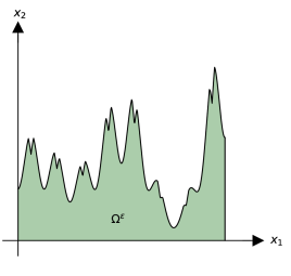
(a)

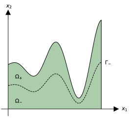
(b)

Figure 3. A locally periodic domain $\Omega^{\varepsilon}$ (a) that satisfies (H2) but not (H1), $\varepsilon=1/8$, and the corresponding homogeneous domain $\Omega$ (b), with $\Gamma_{-}$ marked as a dashed line separating the regions $\Omega_{+}$ and $\Omega_{-}$. The particular function $\eta$ is specified in (28).

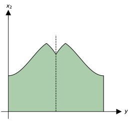
Figure 4. The region below the graph $x_{2}=\eta(1/2,y)$ for $\eta$ given by (28) that satisfies (H2) but not (H1), with symmetry line $y=1/2$ marked with a dashed line.

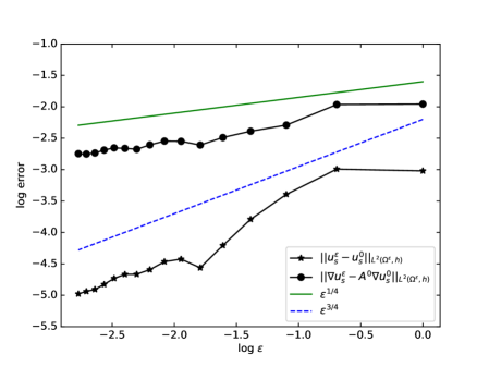
Figure 5. The numerically computed rates of convergence for the approximations $u^{0}$ to $u^{\varepsilon}$, and $A^{0}\nabla u^{0}$ to $\nabla u^{\varepsilon}$, in Theorem 7.1 for $f=1$ and $\Omega^{\varepsilon}$ given by (28) and illustrated for $\varepsilon=1/8$ in Figure 3.

$\varepsilon$	$\|u_{s}^{\varepsilon}-u^{0}_{s}\|_{L^{2}(\Omega^{\varepsilon},\,h)}$	$\|\nabla u_{s}^{\varepsilon}-A^{0}\nabla u^{0}_{s}\|_{L^{2}(\Omega^{\varepsilon},\,h)}$	dof
$0$	–	–	$78\cdot 10^{2}$
$1/1$	$\,\,\,\,0.0488$	$\,\,\,\,0.141$	$39\cdot 10^{3}$
$1/2$	$\,\,\,\,0.0502$	$\,\,\,\,0.140$	$46\cdot 10^{3}$
$1/3$	$\,\,\,\,0.0336$	$\,\,\,\,0.101$	$33\cdot 10^{3}$
$1/4$	$\,\,\,\,0.0226$	$0.0918$	$27\cdot 10^{3}$
$1/5$	$\,\,\,\,0.0149$	$0.0830$	$59\cdot 10^{3}$
$1/6$	$\,\,\,\,0.0104$	$0.0736$	$69\cdot 10^{3}$
$1/7$	$\,\,\,\,0.0120$	$0.0781$	$77\cdot 10^{3}$
$1/8$	$\,\,\,\,0.0115$	$0.0784$	$11\cdot 10^{4}$
$1/9$	$\,\,\,\,0.0101$	$0.0738$	$13\cdot 10^{4}$
$1/10$	$\,0.00941$	$0.0689$	$15\cdot 10^{4}$
$1/11$	$0.00940$	$0.0698$	$20\cdot 10^{4}$
$1/12$	$0.00882$	$0.0704$	$23\cdot 10^{4}$
$1/13$	$0.00801$	$0.0680$	$24\cdot 10^{4}$
$1/14$	$0.00740$	$0.0649$	$35\cdot 10^{4}$
$1/15$	$0.00716$	$0.0638$	$35\cdot 10^{4}$
$1/16$	$0.00688$	$0.0642$	$37\cdot 10^{4}$

Table 1. The numerically computed errors for the approximation in Theorem 6.1, rounded to three significant digits. The number of degrees of freedom, rounded to two significant digits, is abbreviated to dof. The row $\varepsilon=0$ is for the numerical solution $u^{0}_{s}$ to the homogenized problem.

10. A case of non-connected sections

In this section we consider a case where the sections $Y(x)$ are allowed to be disconnected, that is the hypotheses (H1) and (H2) are mildly relaxed. First we describe the weak unfolding limit of the zero extended solutions to problem (2), and then we describe the weak limit in terms of local domain densities using the ideas of Mel’nyk, splitting the oscillating part of the domain into branches (c.f. [27, 28, 43]).

Here, the full unfolded limit domain will be used, denoted by

$$\Omega_{U}=\{(x,y):x\in\Omega,\,y\in Y(x)\},$$

and the effective matrix is given by

$$A^{0} =\begin{pmatrix}\chi_{\Omega_{-}\times\mathbb{T}}&0\\ 0&1\end{pmatrix}.$$ (29)

The limit problem reads

$$-{\mathop{\mathrm{div}}}_{x}(A^{0}\nabla_{x}u) =f\quad\text{ in }\Omega_{U},$$

$$\nabla_{y}u =0\quad\text{ in }\Omega_{U},$$ (30)

$$A^{0}\nabla_{x}u\cdot\nu_{x} =0\quad\text{ on }\partial\Omega_{U}\setminus\Gamma\times\mathbb{T},$$

$$u =0\quad\text{ on }\Gamma\times\mathbb{T},$$

where $\nu_{x}$ denotes the projection of the outward unit normal to $\Omega_{U}$ onto $\mathbb{R}^{2}$. The limit problem (10) is well-posed in the Sobolev space

$$W(\Omega_{U},\Gamma\times\mathbb{T})$$

$$\quad=\{v\in L^{2}(\Omega_{U}):A^{0}\nabla_{x}v\in L^{2}(\Omega_{U}),\,\nabla_{y}v=0\text{ in }\Omega_{U},\,v=0\text{ on }\Gamma\times\mathbb{T}\},$$

equipped with the natural Hilbert space structure.

Theorem 10.1.

Let $u^{\varepsilon}\in H^{1}(\Omega^{\varepsilon},\Gamma)$ be the solutions to problem (2). Let $u^{0}\in W(\Omega_{U},\Gamma\times\mathbb{T})$ be the solution to (10). Then

$$\emph{(i)}\quad\widetilde{u^{\varepsilon}}\rightharpoonup\int_{Y(x)}u^{0}\,dy\quad\text{ weakly in }L^{2}(\Omega),$$

$$\emph{(ii)}\quad\widetilde{\nabla u^{\varepsilon}}\rightharpoonup\int_{Y(x)}A^{0}\nabla_{x}u^{0}\,dy\quad\text{ weakly in }L^{2}(\Omega),$$

as $\varepsilon$ tends to zero.

Proof.

The following a priori estimate holds

$$\|u^{\varepsilon}\|_{H^{1}(\Omega_{-})}+\|T^{\varepsilon}u^{\varepsilon}\|_{L^{2}(\Omega_{u})}+\|T^{\varepsilon}\nabla u^{\varepsilon}\|_{L^{2}(\Omega_{u})} \leq C.$$

There exist

$$u^{0}_{-} \in H^{1}(\Omega_{-},\Gamma),$$

$$u^{0}_{+} \in\big{\{}v\in L^{2}(\Omega_{u}):\frac{\partial v}{\partial x_{2}}\in L^{2}(\Omega_{u}),\,\nabla_{y}v=0\text{ in }\Omega_{u}\big{\}},$$

$$p \in L^{2}(\Omega_{u}),$$

such that, along a subsequence still denoted by $\varepsilon$,

$$u^{\varepsilon} \rightharpoonup u^{0}_{-}\,\,\qquad\qquad\text{ weakly in }H^{1}(\Omega_{-},\,\Gamma),$$

$$T^{\varepsilon}u^{\varepsilon} \rightharpoonup u_{+}^{0}\,\,\qquad\qquad\text{ weakly in }L^{2}(\Omega_{u}),$$

$$T^{\varepsilon}\nabla u^{\varepsilon} \rightharpoonup\big{(}p,\frac{\partial u_{+}^{0}}{\partial x_{2}}\big{)}\qquad\!\!\text{ weakly in }L^{2}(\Omega_{u}).$$

At this point $u_{+}^{0}$ and $p$ depend in general on the fast variable $y$.

The unfolded variational form of problem (7) is by Lemma 5.1,

$$\int_{\Omega_{-}}\nabla u^{\varepsilon}\cdot\nabla\psi\,dx+\int_{\Omega_{u}}T^{\varepsilon}\nabla u^{\varepsilon}\cdot T^{\varepsilon}\nabla\psi\,dxdy =\int_{\Omega_{U}}T^{\varepsilon}f\,T^{\varepsilon}\psi\,dxdy+o(1),$$ (31)

as $\varepsilon$ tends to zero, for any sufficiently smooth $\psi\in H^{1}(\Omega^{\varepsilon},\,\Gamma)$.

Step 1: $p=0$ a.e. in $\Omega_{u}$.

We will show that $p=0$ almost everywhere in $\Omega_{u}$. Let $\phi\in C^{\infty}_{0}(\Omega_{u})$ and consider the sequence of test functions $\varphi^{\varepsilon}(x)=\varepsilon\phi\big{(}x,\frac{x_{1}}{\varepsilon}\big{)}$. Then

$$T^{\varepsilon}\varphi^{\varepsilon} \to 0,$$

$$T^{\varepsilon}\nabla\varphi^{\varepsilon} \to\big{(}\frac{\partial\phi}{\partial y},0\big{)},$$

strongly in $L^{2}(\Omega_{u})$, as $\varepsilon$ tends to zero. By passing to the limit in (31) with test functions $\varphi^{\varepsilon}$ one obtains

$$\int_{\Omega_{u}}p\frac{\partial\phi}{\partial y}\,dxdy =0,\quad\phi\in C^{\infty}_{0}(\Omega_{u}),$$

as $\varepsilon$ tends to zero. That is, $\nabla_{y}p=0$ in $\Omega_{u}$.

Let $\phi\in C^{\infty}_{0}(\Omega_{u})$ be such that $\nabla_{y}\phi=0$. Then consider the sequence of test functions $\varphi^{\varepsilon}$ defined by

$$\varphi^{\varepsilon}(x) =(x_{1}-x_{k}^{\varepsilon})\phi\big{(}x,\frac{x_{1}}{\varepsilon}\big{)},\quad\text{ if }x_{1}\in[x_{k}^{\varepsilon},x_{k+1}^{\varepsilon}),$$

where $x^{\varepsilon}_{k}$ is a tagging such as in (20). Then

$$T^{\varepsilon}\varphi^{\varepsilon} \to 0,$$

$$T^{\varepsilon}\nabla\varphi^{\varepsilon} \to(\phi,0),$$

strongly in $L^{2}(\Omega_{u})$, as $\varepsilon$ tends to zero. By passing to the limit in (31) with test functions $\varphi^{\varepsilon}$ one obtains

$$\int_{\Omega_{u}}p\phi\,dxdy =0,\quad\phi\in C^{\infty}_{0}(\Omega_{u},\nabla_{y}),$$ (32)

as $\varepsilon$ tends to zero. By the density of $C^{\infty}_{0}(\Omega_{u},\nabla_{y})$ in the Sobolev space $\{v\in L^{2}(\Omega_{u}):\nabla_{y}v=0\text{ in }\Omega_{u}\}$, one concludes that (32) holds for $\phi=p$, that is

$$\int_{\Omega_{u}}p^{2}\,dxdy =0.$$

Step 2: Transmission condition.

To determine the transmission condition for $u^{0}_{-}$ and $u^{0}_{+}$ on the internal interface

$$\Gamma_{-}^{u} =\{(x,y):x\in\Gamma_{-},\,y\in Y(x)\},$$

we will trace $u^{\varepsilon}$ from either side.

Let $\phi\in C^{\infty}_{0}(\Omega_{U})$, and set $\phi^{\varepsilon}(x,\frac{x_{1}}{\varepsilon})$.

On the one hand, from below,

$$\int_{\Gamma_{\varepsilon}}u^{\varepsilon}\phi^{\varepsilon}\nu_{2}\,d\sigma =\int_{0}^{1}(\chi_{\Gamma_{\varepsilon}}u^{\varepsilon}\phi^{\varepsilon}\nu_{2})(x_{1},\eta_{-}(x_{1}))\,dx_{1}$$

$$=\int_{0}^{1}\int_{\mathbb{T}}T^{\varepsilon}(\chi_{\Gamma_{\varepsilon}}u^{\varepsilon}\phi\nu_{2})(x_{1},\eta_{-}(x_{1}))\,dy\,dx_{1}$$

$$\to\int_{0}^{1}\int_{\mathbb{T}}(\chi_{Y(x)}u^{0}_{-}\phi\nu_{2})(x_{1},\eta_{-}(x_{1}),y)\,dy\,dx_{1}$$

$$=\int_{\Gamma_{-}}\int_{Y(x)}u^{0}_{-}\phi\nu_{2}\,dy\,d\sigma,$$

as $\varepsilon$ tends to zero, because $T^{\varepsilon}\chi_{\Gamma_{\varepsilon}}(x_{1},\eta_{-}(x_{1}))$ converges to $\chi_{Y(x_{1},\eta_{-}(x_{1}))}(y)$ strongly in $L^{2}((0,1)\times\mathbb{T})$.

On the other hand, from above,

$$\int_{\Gamma_{\varepsilon}}u^{\varepsilon}\phi^{\varepsilon}\nu_{2}\,d\sigma =\int_{\Omega_{u}}T^{\varepsilon}\frac{\partial u^{\varepsilon}}{\partial x_{2}}T^{\varepsilon}\phi^{\varepsilon}\,dxdy+\int_{\Omega_{u}}T^{\varepsilon}u^{\varepsilon}T^{\varepsilon}\frac{\partial\phi^{\varepsilon}}{\partial x_{2}}\,dxdy+o(1)$$

$$\to\int_{\Omega_{u}}\frac{\partial u^{0}_{+}}{\partial x_{2}}\phi\,dxdy+\int_{\Omega_{u}}u^{0}_{+}\frac{\partial\phi}{\partial x_{2}}\,dxdy$$

$$=\int_{\Gamma_{-}}\int_{Y(x)}u^{0}_{+}\phi\nu_{2}\,dy\,d\sigma,$$

as $\varepsilon$ tends to zero.

Thus

$$\int_{\Gamma_{-}}\int_{Y(x)}(u^{0}_{+}-u^{0}_{-})\phi\nu_{2}\,dy\,d\sigma =0,\quad\phi\in C^{\infty}_{0}(\Omega_{U}).$$

It follows that

$$u^{0}_{-} =u^{0}_{+}\quad\text{ in }L^{2}(\Gamma_{-}^{u}),$$ (33)

for by the Lipschitz continuity of $\eta_{-}$,

$$\nu_{2}\geq\frac{1}{\sqrt{1+\max(\eta_{-}^{\prime})^{2}}}>0.$$

The transmission condition (33) means here that the trace of $u^{0}_{+}$ on each connected component of the sections $Y(x)$ for $x\in\Gamma_{-}$ is equal to the trace of $u^{0}_{-}$. That is, zero jump condition into each branch from below.

Step 3: Limit problem.

Let $\varphi\in C^{\infty}(\overline{\Omega_{U}})$ be such that $\nabla_{y}\varphi=0$, and $\varphi$ vanishes on $\Gamma\times\mathbb{T}$. Set $\psi^{\varepsilon}(x)=\varphi(x,\frac{x_{1}}{\varepsilon})$, which belongs to $H^{1}(\Omega^{\varepsilon},\Gamma)$. Using $\psi^{\varepsilon}$ as test functions in (31), one obtains

$$\int_{\Omega_{U}}A^{0}\nabla_{x}u\cdot\nabla_{x}\varphi\,dxdy =\int_{\Omega_{U}}f\varphi\,dxdy,$$ (34)

in the limit as $\varepsilon$ tends to zero, where $u=\chi_{\Omega_{u}}u_{+}^{0}+\chi_{\Omega_{-}\times\mathbb{T}}u_{-}^{0}\in W(\Omega_{U},\Gamma\times\mathbb{T})$ by Step 1. In the upper part $\Omega_{u}$ one uses $p=0$ by Step 2. By the density of the considered set of test functions in $W(\Omega_{U},\Gamma\times\mathbb{T})$, as $\Omega_{U}$ is Lipschitz, one has that $u=u^{0}$ is the unique solution to problem (10). One concludes that the weak convergences (i) and (ii) have been established for the full sequences. ∎

Remark that Lemma 8.1 holds without hypotheses (H1), (H2), by the same argument, and it takes the following form, which is the result that corresponds to Theorem 7.1 in this case.

Lemma 10.1.

Let $u^{\varepsilon}\in H^{1}(\Omega^{\varepsilon},\Gamma)$ be the solutions to (2), and let $u^{0}\in W(\Omega_{U},\Gamma\times\mathbb{T})$ be the solution to (10). Then

(i) $$\quad T^{\varepsilon}u^{\varepsilon}\to u^{0}\quad\text{ strongly in }L^{2}(\Omega_{U}),$$

(ii) $$\quad T^{\varepsilon}\nabla u^{\varepsilon}\to\big{(}\chi_{\Omega_{-}\times\mathbb{T}}\frac{\partial u^{0}}{\partial x_{1}},\frac{\partial u^{0}}{\partial x_{2}}\big{)}\quad\text{ strongly in }L^{2}(\Omega_{U}),$$

as $\varepsilon$ tends to zero.

We will conclude this section by translating the limit problem (10) into a system in the original coordinates $x\in\Omega$, ($\overline{\Omega}$ is the Hausdorff limit of $\overline{\Omega^{\varepsilon}}$), in a particular case of a finite number of ’bumps’ on the boundary.

Lemma 10.2.

Let $\omega$ be an open set in $\mathbb{R}^{N}$. Then there exists an open cover $K^{\prime}$ of $\omega$ such that for all $v\in L^{2}(\omega)$ with $\nabla_{x^{\prime}}v=0$ almost everywhere in $\omega$, $(x,x^{\prime})\in\omega$, one has that $v$ is constant in $x^{\prime}$ almost everywhere in each $V\in K^{\prime}$.

Proof.

A subset $V$ of $\omega$ is said to have the property $(P)$ if the intersection of $V$ and any $k$-plane parallel to the $x^{\prime}$-coordinate $k$-planes is connected, $x^{\prime}\in\mathbb{R}^{k}$. For $(x,x^{\prime})\in\omega$, let $V(x,x^{\prime})$ be a neighborhood of $(x,x^{\prime})$ in $\omega$ that is not contained in any distinct neighborhood of $(x,x^{\prime})$ in $\omega$ with the property (P). By the Zorn lemma, at least one such maximal element exists for the set inclusion partial order on the set of all neighborhoods of $(x,x^{\prime})$ with the property (P), because $\omega$ is open and if $F$ is a totally ordered subset, $\cup_{V\in F}V$ is an upper bound for $F$. Then $K^{\prime}=\{V(x,x^{\prime}):(x,x^{\prime})\in\omega\}$ is an open cover of $\omega$.

Let $v\in L^{2}(\omega)$ be such that $\nabla_{x^{\prime}}v=0$ almost everywhere in $\omega$. Then $v$ has a representative $\tilde{v}$ that is absolutely continuous on almost all line segments parallel to the $x^{\prime}$-coordinate axes and whose classical partial derivatives parallel to the $x^{\prime}$-coordinate axes belong to $L^{2}(\omega)$. It follows from Fubini’s theorem that $\tilde{v}$ assumes constant value on each connected component of each $k$-plane parallel to the $x^{\prime}$-coordinate $k$-planes when intersected with $\omega$. Therefore $v$ is constant in $x^{\prime}$ almost everywhere on each $V\in K^{\prime}$. ∎

Now we restrict to domains such that there is a finite open cover of $\Omega_{U}$ as in Lemma 10.2 with $\omega=\Omega_{U}$ and $x^{\prime}=y$, effectively discarding domains with a countably infinite number of ’bumps’ on the boundary. For instance, excluding $\eta(x,y)=x_{1}^{2}\sin(\frac{y}{x_{1}})$, and $\eta(x,y)={\mathop{\mathrm{dist}}}(y,K)$, where $K$ is a Cantor set.

We say that $K$ is a partition of an open set $\omega$ in $\mathbb{R}^{N}$ if $K$ consists of disjoint nonempty open subsets of $\omega$ such that $\overline{\omega}=\cup_{V\in K}\overline{V}$. Under the assumption that there is a finite open cover $K^{\prime}$ of $\Omega_{U}$ as in Lemma 10.2, we can construct a finite partition $K$ of $\Omega_{U}$ as follows. Given $K^{\prime}=\{V_{1},\ldots,V_{k}\}$, let $K=\{V_{1},V_{2}\setminus\overline{V_{1}},\ldots,V_{k}\setminus\cup_{j=1}^{k-1}\overline{V_{j}}\}$.

Let $K$ be a finite partition of $\Omega_{U}$ with the same property as the open cover in Lemma 10.2. Denote the measure of the connected components of $Y(x)$ by

$$h_{V} =|Y(x)\cap\{y:(x,y)\in V\}|,$$

for $V\in K$, that is the density of $\Omega^{\varepsilon}$ in $\Omega$. Denote the common boundaries of the subdomains $U,V\in K$ of the partition by

$$\Gamma_{U,V} =\partial U\cap\partial V.$$

Let the effective matrix be given by

$$A^{0} =\begin{pmatrix}\chi_{\Omega_{-}}&0\\ 0&1\end{pmatrix}.$$

Let

$$W_{K}=\big{\{}\,\{v_{V}\}_{V\in K}:\,\, v_{V}\in L^{2}(\pi_{\mathbb{R}^{2}}V,h_{V}),$$

$$A^{0}\nabla v_{V}\in L^{2}(\pi_{\mathbb{R}^{2}}V,h_{V}),$$

$$[v]=0\text{ on }\pi_{\mathbb{R}^{2}}\Gamma_{U,V},$$

$$v_{V}=0\text{ on }\Gamma\cap\pi_{\mathbb{R}^{2}}\overline{V},$$

$$U,V\in K\,\big{\}},$$

where $\pi_{\mathbb{R}^{2}}$ denotes the projection onto $\mathbb{R}^{2}$, equipped with the natural Hilbert space structure.

The limit problem

$$-{\mathop{\mathrm{div}}}(h_{V}A^{0}\nabla u_{V}) =h_{V}f\quad\text{ in }\pi_{\mathbb{R}^{2}}V,$$

$$u_{V} =0\qquad\,\,\text{ on }\Gamma\cap\pi_{\mathbb{R}^{2}}\overline{V},$$

$$h_{V}A^{0}\nabla u_{V}\cdot\nu =0\qquad\,\,\text{ on }(\partial\Omega\setminus\Gamma)\cap\pi_{\mathbb{R}^{2}}\overline{V},$$ (35)

$$[u] =0\qquad\,\,\text{ on }\pi_{\mathbb{R}^{2}}\Gamma_{U,V},$$

$$[hA^{0}\nabla u\cdot\nu] =0\qquad\,\,\text{ on }\pi_{\mathbb{R}^{2}}\Gamma_{U,V},$$

is then well-posed in $W_{K}$.

Corollary 10.1.

Let $u^{\varepsilon}\in H^{1}(\Omega^{\varepsilon},\Gamma)$ be the solutions to (2), and let $u^{0}\in W(\Omega_{U},\Gamma\times\mathbb{T})$ be the solution to (10). Let $K$ be a finite partition of $\Omega_{U}$ with the same property as the open cover in Lemma 10.2 with $\omega=\Omega_{U}$ and $x^{\prime}=y$. Then

(i) $$\quad\widetilde{u^{\varepsilon}}\rightharpoonup\sum_{V\in K}h_{V}\chi_{\pi_{\mathbb{R}^{2}}V}u^{0}\big{|}_{V}\quad\text{ weakly in }L^{2}(\Omega),$$

(ii) $$\quad\widetilde{\nabla u^{\varepsilon}}\rightharpoonup\sum_{V\in K}h_{V}\chi_{\pi_{\mathbb{R}^{2}}V}A^{0}\nabla u^{0}\big{|}_{V}\quad\text{ weakly in }L^{2}(\Omega),$$

as $\varepsilon$ tends to zero. Moreover, $u^{0}=u_{V}^{0}$ in $V\in K$, where $\{u_{V}^{0}\}_{V\in K}$ in $W_{K}$ is the solution to (10).

Proof.

It follows from the weak unfolding convergence $T^{\varepsilon}u^{\varepsilon}\rightharpoonup u^{0}$ in $L^{2}(\Omega_{U})$, that

$$\widetilde{u^{\varepsilon}} \rightharpoonup\int_{Y(x)}u^{0}\,dy=\int_{Y(x)}\sum_{V\in K}\chi_{V}u^{0}\,dy=\sum_{V\in K}h_{V}\chi_{\pi_{\mathbb{R}^{2}}V}u^{0}\big{|}_{V},$$

as $\varepsilon$ tends to zero. The same computation gives the convergence of the flows. By writing $u^{0}=\sum_{V\in K}\chi_{V}u^{0}$, one verifies that the limit problem (10) is equivalent to the limit problem (10) with $u_{V}^{0}=\chi_{V}u^{0}$ on $V$, for any suitable partition $K$. ∎

References

- [1] S. Aiyappan, A. K. Nandakumaran, and R. Prakash. Generalization of unfolding operator for highly oscillating smooth boundary domains and homogenization. Calc. Var. Partial Differential Equations, 57(3):Art. 86, 30, 2018.
- [2] S. Aiyappan, A. K. Nandakumaran, and R. Prakash. Semi-linear optimal control problem on a smooth oscillating domain. Commun. Contemp. Math., 22(4):1950029, 26, 2020.
- [3] E. Akimova, S. Nazarov, and G. Chechkin. Asymptotics of the solution of the problem of deformation of an arbitrary locally periodic thin plate. Transactions of the Moscow Mathematical Society, 65:1–29, 2004.
- [4] G. Allaire. Homogenization and two-scale convergence. SIAM Journal on Mathematical Analysis, 23(6):1482–1518, 1992.
- [5] Y. Amirat, O. Bodart, U. De Maio, and A. Gaudiello. Asymptotic approximation of the solution of the laplace equation in a domain with highly oscillating boundary. SIAM journal on mathematical analysis, 35(6):1598–1616, 2004.
- [6] J. M. Arrieta and M. C. Pereira. Homogenization in a thin domain with an oscillatory boundary. Journal de Mathématiques Pures et Appliquées, 96(1):29–57, 2011.
- [7] J. M. Arrieta and M. Villanueva-Pesqueira. Unfolding operator method for thin domains with a locally periodic highly oscillatory boundary. SIAM J. Math. Anal., 48(3):1634–1671, 2016.
- [8] J. M. Arrieta and M. Villanueva-Pesqueira. Thin domains with non-smooth periodic oscillatory boundaries. J. Math. Anal. Appl., 446(1):130–164, 2017.
- [9] I. Babuska. Solutions of interface problems by homogenization. SIAM J. Math. Anal., Part 1, 7(5):603-634; Part 2, 7(5):635-645; Part 3 8(6):923-937,1976.
- [10] N. S. Bakhvalov. Averaged characteristics of bodies with periodic structure. In Doklady Akademii Nauk, volume 218(5), pages 1046–1048. Russian Academy of Sciences, 1974.
- [11] N. S. Bakhvalov. Averaging of nonlinear partial differential equations with rapidly oscillating coefficients. In Doklady Akademii Nauk, volume 225(2), pages 249–252. Russian Academy of Sciences, 1975.
- [12] N. S. Bakhvalov. Averaging of partial differential equations with rapidly oscillating coefficients. In Doklady Akademii Nauk, volume 221(3), pages 516–519. Russian Academy of Sciences, 1975.
- [13] N. S. Bakhvalov and G. Panasenko. Homogenisation of processes in periodic media. Nauka, Moscow, 1984.
- [14] O. A. Bakhvalov. On convergence of solutions of elliptic and parabolic equations when coefficients weakly converge. In Uspekhi mat. nauk, volume 30(4), pages 257–258, 1975.
- [15] J. M. Ball. Some open problems in elasticity. In Geometry, mechanics, and dynamics, pages 3–59. Springer, 2002.
- [16] V. L. Berdichevsky. Spacial homogenization of periodic structures. In Dokl. Akad Nauk SSSR, volume 222(3), pages 565–567. Russian Academy of Sciences, 1975.
- [17] D. Blanchard, A. Gaudiello, and G. Griso. Junction of a periodic family of elastic rods with a 3d plate. part I. Journal de mathématiques pures et appliquées, 88(1):1–33, 2007.
- [18] D. Blanchard, A. Gaudiello, and G. Griso. Junction of a periodic family of elastic rods with a thin plate. part II. Journal de mathématiques pures et appliquées, 88(2):149–190, 2007.
- [19] D. Borisov and P. Freitas. Asymptotics of dirichlet eigenvalues and eigenfunctions of the laplacian on thin domains in rd. Journal of Functional Analysis, 258(3):893–912, 2010.
- [20] R. Brizzi and J.-P. Chalot. Homogénéisation de frontiére. Thése, Université de Nice, 1978.
- [21] R. Brizzi and J.-P. Chalot. Boundary homogenization and Neumann boundary value problem. Ricerche di Matematica, 46(2):341–388, 1997.
- [22] G. A. Chechkin, A. Friedman, and A. L. Piatnitski. The boundary-value problem in domains with very rapidly oscillating boundary. Journal of Mathematical Analysis and Applications, 231(1):213–234, 1999.
- [23] D. Cioranescu, A. Damlamian, and G. Griso. Periodic unfolding and homogenization. Comptes Rendus Mathematique, 335(1):99–104, 2002.
- [24] D. Cioranescu, A. Damlamian, and G. Griso. The periodic unfolding method in homogenization. SIAM Journal on Mathematical Analysis, 40(4):1585–1620, 2008.
- [25] D. Cioranescu, A. Damlamian, and G. Griso. The Periodic Unfolding Method: Theory and Applications to Partial Differential Problems, volume 3. Springer, 2018.
- [26] A. Damlamian and K. Pettersson. Homogenization of oscillating boundaries. Discrete Contin. Dyn. Syst., 23(1-2):197–210, 2009.
- [27] U. De Maio, T. Durante, and T. A. Mel’Nyk. Asymptotic approximation for the solution to the robin problem in a thick multi-level junction. Mathematical Models and Methods in Applied Sciences, 15(12):1897–1921, 2005.
- [28] T. Durante and T. A. Mel’nyk. Homogenization of quasilinear optimal control problems involving a thick multilevel junction of type 3: 2: 1. ESAIM: Control, Optimisation and Calculus of Variations, 18(02):583–610, 2012.
- [29] A. C. Esposito, P. Donato, A. Gaudiello, and C. Picard. Homogenization of the p-laplacian in a domain with oscillating boundary. Comm. Appl. Nonlinear Anal, 4(4):1–23, 1997.
- [30] A. Gaudiello. Asymptotic behaviour of non-homogeneous Neumann problems in domains with oscillating boundary. Ricerche di Matematica, 43(2):239–292, 1994.
- [31] A. Gaudiello, O. Guibé, and F. Murat. Homogenization of the brush problem with a source term in . Arch. Ration. Mech. Anal., 225(1):1–64, 2017.
- [32] A. Gaudiello and T. A. Mel’nyk. Homogenization of a nonlinear monotone problem with nonlinear Signorini boundary conditions in a domain with highly rough boundary. J. Differential Equations, 265(10):5419–5454, 2018.
- [33] A. Gaudiello and T. A. Mel’nyk. Homogenization of a nonlinear monotone problem with a big nonlinear signorini boundary interaction in a domain with highly rough boundary. Nonlinearity, 32(12):5150, 2019.
- [34] F. Hecht. New development in freefem++. Journal of numerical mathematics, 20(3-4):251–266, 2012.
- [35] V. V. Jikov, S. M. Kozlov, and O. A. Oleinik. Homogenization of differential operators and integral functionals. Springer-Verlag, Berlin, 1994.
- [36] A. Kufner. Weighted sobolev spaces, volume 31. John Wiley & Sons Incorporated, 1985.
- [37] A. Kufner and A.-M. Sändig. Some applications of weighted Sobolev spaces, volume 100. Springer, 1987.
- [38] R. Lipton and M. Avellaneda. Darcy’s law for slow viscous flow past a stationary array of bubbles. Proceedings of the Royal Society of Edinburgh Section A: Mathematics, 114(1-2):71–79, 1990.
- [39] R. Mahadevan, A. K. Nandakumaran, and R. Prakash. Homogenization of an elliptic equation in a domain with oscillating boundary with non-homogeneous non-linear boundary conditions. Applied Mathematics & Optimization, pages 1–34, 2018.
- [40] V. A. Marchenko and E. Y. Khruslov. Boundary-value problems with fine-grained boundary. Matematicheskii Sbornik, 107(3):458–472, 1964.
- [41] T. A. Mel’nyk. Homogenization of the poisson equation in a thick periodic junction. Zeitschrift für Analysis und ihre Anwendungen, 18(4):953–975, 1999.
- [42] T. A. Mel’nyk. Homogenization of a boundary-value problem with a nonlinear boundary condition in a thick junction of type 3: 2: 1. Math. Methods Appl. Sci., 31(9):1005–1027, 2008.
- [43] T. A. Mel’nyk. Asymptotic approximation for the solution to a semi-linear parabolic problem in a thick junction with the branched structure. Journal of Mathematical Analysis and Applications, 424(2):1237–1260, 2015.
- [44] T. A. Mel’nyk and S. A. Nazarov. Asymptotics of the neumann spectral problem solution in a domain of ’thick comb’ type. J. Math. Sci, 85(6):2326–2346, 1997.
- [45] T. A. Mel’nyk and A. V. Popov. Asymptotic analysis of boundary-value problems in thin perforated domains with rapidly varying thickness. Nonlinear oscillations, 13(1):57–84, 2010.
- [46] A. K. Nandakumaran, R. Prakash, and B. C. Sardar. Homogenization of an optimal control via unfolding method. SIAM Journal on Control and Optimization, 53(5):3245–3269, 2015.
- [47] S. A. Nazarov. Asymptotic theory of thin plates and rods. vol. 1. dimension reduction and integral estimates. Nauchnaya Kniga, 2001.
- [48] G. Nguetseng. A general convergence result for a functional related to the theory of homogenization. SIAM Journal on Mathematical Analysis, 20(3):608–623, 1989.
- [49] O. A. Oleinik, A. S. Shamaev, and G. A. Yosifian. Mathematical problems in elasticity and homogenization. North-Holland, Amsterdam, 1992.
- [50] G. Papanicolau, A. Bensoussan, and J.-L. Lions. Asymptotic analysis for periodic structures, volume 5. Elsevier, 1978.
- [51] I. Pettersson. Two-scale convergence in thin domains with locally periodic rapidly oscillating boundary. Differential Equations & Applications, 9(3):393–412, 2017.
- [52] E. Sánchez-Palencia. Non-homogeneous media and vibration theory. Lecture notes in physics, 127, 1980.
- [53] E. Spagnolo and S. De Giorgi. Sulla convergenza degli integrali dellenergia per operatori ellittici del secondo ordine. Boll. Unione Mat. Ital. 8, pages 391–411, 1973.
- [54] L. Tartar. Problemes dhomogeneisation dans les equations aux derivees partielles. Cours Peccot, College de France, 1977.
- [55] V. V. Zhikov. On two-scale convergence. Journal of Mathematical Sciences, 120(3):1328–1352, 2004.