Symmetries of complex analytic vector fields with an essential singularity on the Riemann sphere

Abstract.

We consider the family

${\mathscr{E}}(s,r,d)=\Big{\{}X(z)=\frac{Q(z)}{P(z)}\ {\text{\myfont e}}^{E(z)}\frac{\partial}{\partial z}\Big{\}},$

with $Q,P,E$ polynomials, $\deg{Q}=s$, $\deg{P}=r$ and $\deg{E}=d$, of singular complex analytic vector fields $X$ on the Riemann sphere ${\widehat{\mathbb{C}}}$. For $d\geq 1$, $X\in{\mathscr{E}}(s,r,d)$ has $s$ zeros and $r$ poles on the complex plane and an essential singularity at infinity. Using the pullback action of the affine group $Aut({\mathbb{C}})$ and the divisors for $X$, we calculate the isotropy groups $Aut({\mathbb{C}})_{X}$ and the discrete symmetries for $X\in{\mathscr{E}}(s,r,d)$. Each subfamily ${\mathscr{E}}(s,r,d)_{id}$, of those $X$ with trivial isotropy group in $Aut({\mathbb{C}})$, is endowed with a holomorphic trivial principal $Aut({\mathbb{C}})$–bundle structure. Necessary and sufficient conditions in order to ensure the equality ${\mathscr{E}}(s,r,d)={\mathscr{E}}(s,r,d)_{id}$ and those $X\in{\mathscr{E}}(s,r,d)$ with non–trivial isotropy are realized. Explicit global normal forms for $X\in{\mathscr{E}}(s,r,d)$ are presented. A natural dictionary between vector fields, 1–forms, quadratic differentials and functions is extended to include the presence of non–trivial discrete symmetries $\Gamma<Aut({\mathbb{C}})$.

1. Introduction

Meromorphic vector fields on compact Riemann surfaces are well understood, at least on some aspects: see [27], [28], [8], [18], [31]. Essential singularities represent the next level of complexity.

We study the holomorphic families consisting of singular complex analytic vector fields on the Riemann sphere ${\widehat{\mathbb{C}}}$ with a singular set composed of $s\geq 0$ zeros and $r\geq 0$ poles on ${\mathbb{C}}$, and an isolated essential singularity at $\infty\in{\widehat{\mathbb{C}}}$ of 1–order $d\geq 1$ namely

$${\mathscr{E}}(s,r,d)=\left\{X(z)=\frac{Q(z)}{P(z)}\ {\text{\myfont e}}^{E(z)}\frac{\partial}{\partial z}\ \Big{|}\ \begin{array}[]{l}Q,\ P,\ E\in{\mathbb{C}}[z],\\ \deg{Q}=s,\ \deg{P}=r,\ \deg{E}=d\end{array}\right\}.$$

The associated families of functions

$$\left\{\Psi_{X}(z)=\int^{z}\frac{P(\zeta)}{Q(\zeta)}\ {\text{\myfont e}}^{-E(\zeta)}d\zeta\ \Big{|}\ X\in{\mathscr{E}}(s,r,d)\right\}$$

and their Riemann surfaces $\{{\mathcal{R}}_{X}\}$ are part of the transcendental functions described in R. Nevanlinna’s seminal work; see [30] and [29] particularly ch. XI. Recently, M. Taniguchi studied these families $\{\Psi_{X}\}$ from the viewpoint of deformation of functions, see [32] and [33]. Motivated by complex dynamics, K. Biswas and R. Pérez–Marco, [6], [7], enrich the study of $\{\Psi_{X}\}$ and $\{{\mathcal{R}}_{X}\}$. In [4] the authors explored the family of vector fields ${\mathscr{E}}(0,0,d)$, obtaining an analytic classification as well as presenting analytic normal forms for $d\leq 3$.

The search for a natural/adequate notion of normal form for vector fields in ${\mathscr{E}}(s,r,d)$ leads to novel paths. A characteristic of the study of vector fields on the Riemann sphere, or on the affine plane, is that their group of automorphisms is a finite dimensional complex analytic Lie group: rich enough and yet treatable. For $d\geq 1$ the essential singularity of $X\in{\mathscr{E}}(s,r,d)$ provides a marked point at $\infty\in{\widehat{\mathbb{C}}}$. We consider the canonical action

$\mathcal{A}:Aut({\mathbb{C}})\times{\mathscr{E}}(s,r,d)\longrightarrow{\mathscr{E}}(s,r,d),\ \ \ (T,X)\longmapsto T^{*}X$,

of the affine transformation group $Aut({\mathbb{C}})$ corresponding to those $T\in Aut({\widehat{\mathbb{C}}})=PSL(2,{\mathbb{C}})$ that fix $\infty$.

Our pourpose is the study of the quotient spaces ${\mathscr{E}}(s,r,d)/Aut({\mathbb{C}})$.

Clearly it is a valuable and accurate tool for understanding the dynamics of the vector fields $X\in{\mathscr{E}}(s,r,d)$ and their associated families of functions $\{\Psi_{X}\,|\,X\in{\mathscr{E}}(s,r,d)\}$.

The action $\mathcal{A}$ determines the following natural classification problems:

1. Characterize under which conditions $X_{1}$ and $X_{2}$ in ${\mathscr{E}}(s,r,d)$ are complex analytically equivalent, i.e. whether there exist $T\in Aut({\mathbb{C}})$ such that

   $X_{2}\xrightarrow{\ T^{*}}X_{1}$.

2. Considering the singular flat metric $({\widehat{\mathbb{C}}},g_{X})$ associated to $X$, characterize under which conditions the metrics associated to $X_{1}$ and $X_{2}$ in ${\mathscr{E}}(s,r,d)$ are isometrically equivalent; i.e. whether there exist $(T,{\text{\myfont e}}^{i\theta})\in Aut({\mathbb{C}})\times\mathbb{S}^{1}$ such that

   $({\widehat{\mathbb{C}}},g_{X_{2}})\xrightarrow{\ T^{*}}({\widehat{\mathbb{C}}},g_{{\text{\myfont e}}^{i\theta}X_{1}})$,

   is an isometry, where ${\text{\myfont e}}^{i\theta}:X\mapsto{\text{\myfont e}}^{i\theta}X$ acts by rotations. For the description of the metrics see [28], [27], [4] and the singular complex analytic dictionary Proposition 4.1.

The relation between (AC) and (MC), see Lemma 2.4 for further detail, determines the following diagram

where $\pi_{1}$, $\pi_{2}$ are the natural projections to equivalence classes.

As a first step to enlighten both classifications, we study the $Aut({\mathbb{C}})$–fibre bundle structure on ${\mathscr{E}}(s,r,d)$. Let

${\mathscr{E}}(s,r,d)_{id}\subseteq{\mathscr{E}}(s,r,d)$

denote those $X$ with trivial isotropy group $Aut({\mathbb{C}})_{X}\subset Aut({\mathbb{C}})$.

Main Theorem (Analytical and metric classification of ${\mathscr{E}}(s,r,d)$).

1. The families ${\mathscr{E}}(s,r,d)$ and ${\mathscr{E}}(s,r,d)_{id}$ coincide if and only if
   $\bullet\ \gcd(d,s-r-1)=1$, or
   $\bullet\ {\tt k}\not|s$ and ${\tt k}\not|r$, for all non–trivial common divisors ${\tt k}$ of $d$ and $(s-r-1)$.

2. For $s+r+d\geq 2$ and $d\geq 1$, the holomorphic (resp. real analytic) principal bundles

   are trivial. Moreover

   $\bullet\ {\mathscr{E}}(s,r,d)_{id}/Aut({\mathbb{C}})$ has complex dimension $s+r+d-1$,

   $\bullet\ {\mathscr{E}}(s,r,d)_{id}/(Aut({\mathbb{C}})\times\mathbb{S}^{1})$ has real dimension $2(s+r+d)-3$ and

   both quotients are compact when ${\mathscr{E}}(s,r,d)={\mathscr{E}}(s,r,d)_{id}$.

A natural tool for the study of $X$ is the divisor

$$\underbrace{[q_{1},\ldots,q_{s}]}_{{\mathcal{Z}}},\underbrace{[p_{1},\ldots,p_{r}]}_{{\mathcal{P}}},\underbrace{[e_{1},\ldots,e_{d}]}_{{\mathcal{E}}},$$

consisting of the roots of $Q(z)$, $P(z)$ and $E(z)$, see Definition 2.1. Some remarkable and novel features of ${\mathscr{E}}(s,r,d)$ are that

$\bullet$ $\left({\mathcal{Z}}\cup\,{\mathcal{P}}\right)\cap\,{\mathcal{E}}$ need not be empty, and

$\bullet$ ${\mathcal{E}}$ is not part of the singular set of the phase portrait of ${\mathfrak{Re}\left(X\right)}$.

In order to show that ${\mathscr{E}}(s,r,d)_{id}$ is a holomorphic trivial principal $Aut({\mathbb{C}})$–bundle, in Lemma 2.12, we exhibit explicit global sections

$\sigma:{\mathscr{E}}(s,r,d)_{id}/Aut({\mathbb{C}})\longrightarrow{\mathscr{E}}(s,r,d)_{id}$.

We further localize the singular locus of the quotient ${\mathscr{E}}(s,r,d)/Aut({\mathbb{C}})$, leading to a natural question:

“How can we construct complex analytic vector fields $X\in{\mathscr{E}}(s,r,d)$ such that $\Gamma$ concides with the symmetries $Aut({\mathbb{C}})_{X}$ or is a proper subgroup of it?”

Theorem ($\Gamma$–symmetry).

Let $\Gamma$ be a non–trivial subgroup of $Aut({\mathbb{C}})$. A vector field $X\in{\mathscr{E}}(s,r,d)$ is $\Gamma$–symmetric if and only if $\Gamma$ is a discrete rotation group and

1. $\gcd(d,s-r-1)\neq 1$,

2. all three subsets of the divisor $[q_{1},\ldots,q_{s}]$, $[p_{1},\ldots,p_{r}]$, $[e_{1},\ldots,e_{d}]$ of $X$ are $\Gamma$–invariant.

This result can be found restated as Theorem 2.15 in the text, where an additional equivalent characterization is given. It is clear that condition (2) is necessary, however it comes as a (pleasant) surprise that condition (1) provides sufficiency; compare with the case of $\Gamma$–symmetric rational functions [15] § 5 and $\Gamma$–symmetric rational vector fields [3].

The explicit global sections found in Lemma 2.12 provide global normal forms for vector fields $X\in{\mathscr{E}}(s,r,d)_{id}$, see Definition 3.1 and Corollary 3.2. The normal forms are global in the sense that the explicit expressions for $\sigma([X])$ are valid:

$\bullet$ for the whole family ${\mathscr{E}}(s,r,d)_{id}/Aut({\mathbb{C}})$, and

$\bullet$ on the whole Riemann sphere ${\widehat{\mathbb{C}}}$, when considering the phase portraits of ${\mathfrak{Re}\left(X\right)}$.

Furthermore an application of Theorem 2.15 allows us to realize those $X\in{\mathscr{E}}(s,r,d)$ with non–trivial isotropy, thus providing normal forms for all $X\in{\mathscr{E}}(s,r,d)$.

The above considerations lead to the following question.

“What is the relationship/link between vector fields and functions, specifically between the families ${\mathscr{E}}(s,r,d)$ and $\{\Psi_{X}\,|\,X\in{\mathscr{E}}(s,r,d)\}$?”

To answer this, consider an arbitrary Riemann surface $M$ (not necessarily compact). In accordance with [23], [28], [27] and [4], we present a Dictionary explaining the naturality and the richness of the theory: a statement in one context can be restated in any other.

Theorem (The dictionary under $\Gamma$–symmetry).

Let $\Gamma$ be a subgroup of $Aut(M)$ having quotient $proj:M\longrightarrow M/\Gamma$ to a Riemann surface.

On $M$ there is a canonical one to one correspondence between:

1. $\Gamma$–symmetric singular complex analytic vector fields $X$.

2. $\Gamma$–symmetric singular complex analytic differential forms $\omega_{X}$, satisfying $\omega_{X}(X)\equiv 1$.

3. $\Gamma$–symmetric singular complex analytic orientable quadratic differentials $\omega_{X}\otimes\omega_{X}$.

4. $\Gamma$–symmetric singular flat metrics $(M,g_{X})$ with suitable singularities.

5. $\Gamma$–symmetric global singular complex analytic (possibly multivalued) distinguished parameters $\Psi_{X}$.

6. Pairs $\big{(}{\mathcal{R}}_{X},\pi^{*}_{X,2}(\frac{\partial}{\partial t})\big{)}$ consisting of branched Riemann surfaces ${\mathcal{R}}_{X}$, associated to the $\Gamma$–symmetric maps $\Psi_{X}$.

A more complete statement is provided as Theorem 4.2 and the calculation of the singularites of $Y=proj_{*}X$, for $X\in{\mathscr{E}}(s,r,d)$ is performed in Proposition 4.3 and Table 1.

The groups of symmetries $\Gamma$ of Riemann surfaces and their $\Gamma$–symmetric holomorphic tensors have been the subject of study in different works from their own perspective. F. Klein was a pioneer [24], for more recent work see [1], [17] ch. V, [9] for the general theory of automorphisms $Aut(M)$ and spaces of differentials, [15] §5 for invariant rational functions on ${\widehat{\mathbb{C}}}$; and references therein.

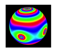
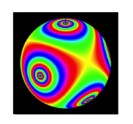
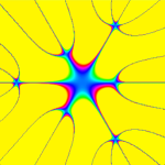
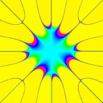
In our case, examples of $\Gamma$–symmetric vector fields of the following kinds: rational, vector fields $X\in{\mathscr{E}}(s,r,d)$, and vector fields on the torus $\mathbb{T}$ are presented. See Figures 4, 1, and 5, respectively.

In Proposition 4.3 and Remark 4.4, the geometrical meaning of the subgroups $\Gamma<Aut({\mathbb{C}})$ that leave invariant $X\in{\mathscr{E}}(s,r,d)$ is studied by considering the natural projection $proj:{\widehat{\mathbb{C}}}\longrightarrow{\widehat{\mathbb{C}}}/\Gamma$ and the associated vector fields $proj_{*}X$ on ${\widehat{\mathbb{C}}}/\Gamma$.

The authors wish to thank Adolfo Guillot for useful comments.

2. $Aut({\mathbb{C}})$–fibre bundle structure on ${\mathscr{E}}(s,r,d)$

We work in the singular complex analytic category. Recalling definition 2.1 of [4], for our present purposes; a singular analytic vector field on ${\widehat{\mathbb{C}}}_{z}$ is a holomorphic vector field $X$ on ${\widehat{\mathbb{C}}}_{z}\backslash Sing(X)$, with singular set $Sing(X)$ consisting of: zeros denoted by ${\mathcal{Z}}$; poles denoted by ${\mathcal{P}}$; isolated essential singularity at $\infty\in{\widehat{\mathbb{C}}}$.

Because of Picard’s theorem, even the local description of essential singularities of functions leads to a global study, see for instance [4] pp. 129. Due to the diversity and wildness of essential singularities, a first step in understanding them is to restrict ourselves to the tame family ${\mathscr{E}}(s,r,d)$.

This section is devoted to the proof of the Main Theorem:

In §2.1 we provide explicit coordinates for ${\mathscr{E}}(s,r,d)$ that facilitate the work to be done. In §2.2 we present the action of $Aut({\mathbb{C}})$ on ${\mathscr{E}}(s,r,d)$ and prove that ${\mathscr{E}}(s,r,d)_{id}$ is a trivial principal $Aut({\mathbb{C}})$–bundle. Finally in §2.3 the arithmetic condition “${\tt k}\not|q$ and ${\tt k}\not|r$, for all non–trivial common divisors ${\tt k}$ of $d$ and $(s-r-1)$ implies that ${\mathscr{E}}(s,r,d)={\mathscr{E}}(s,r,d)_{id}$” is addressed.

2.1. Coordinates for ${\mathscr{E}}(s,r,d)$

Viète’s map provides a parametrization of the space of monic polynomials of degree $s\geq 1$ by the roots $\{q_{i}\}_{i=1}^{s}$, up to the action of the symmetric group of order $s$, $Sym(s)$. By parametrization we understand an atlas with appropriate charts; for instance in the case of the parametrization by roots, this is valid for neighborhoods that avoid multiple roots. It will be useful to allow non–monic polynomials in the description of $X\in{\mathscr{E}}(s,r,d)$, explicitly

$$Q(z)=\lambda\,(z-q_{1})\cdots(z-q_{s}) :=\lambda\,(z^{s}+a_{1}z^{s-1}+\cdots+a_{s}),$$

$$P(z)=(z-p_{1})\cdots(z-p_{r}) :=z^{r}+b_{1}z^{r-1}+\cdots+b_{r},$$

$$E(z)=c_{0}\,(z-e_{1})\cdots(z-e_{d}) :=c_{0}\,\big{(}z^{d}+(c_{1}/c_{0})z^{d-1}+\cdots+(c_{d}/c_{0})\big{)}.$$

Definition 2.1.

The divisor of $X\in{\mathscr{E}}(s,r,d)$ is

$$\underbrace{[q_{1},\ldots,q_{s}]}_{{\mathcal{Z}}},\underbrace{[p_{1},\ldots,p_{r}]}_{{\mathcal{P}}},\underbrace{[e_{1},\ldots,e_{d}]}_{{\mathcal{E}}},$$

the unordered configuration of the roots of $Q(z)$, $P(z)$ and $E(z)$.

Obviously we assume ${\mathcal{Z}}\cap{\mathcal{P}}=\varnothing$, however, $\left({\mathcal{Z}}\cup\,{\mathcal{P}}\right)\cap\,{\mathcal{E}}$, need not be empty. Different versions of the moduli space of $n$ points on the Riemann sphere under the action of $SL(2,{\mathbb{C}})$ are currently considered in the literature by using Mumford’s geometric invariant theory GIT, see for instance [13], [21] and references therein. In our case we consider $s+r+d$ unordered points with three “flavors”.

The naturality of the divisors should come as no surprise: in fact for $X\in{\mathscr{E}}(s,r,d)$ there is an identification between the zero dimensional object (the divisor) and the one dimensional object (the singular analytic vector field), see [34] for other examples of the same phenomena.

Proposition 2.2.

The complex manifold ${\mathscr{E}}(s,r,d)$ can be parametrized by:

1. The $s+r+d+2$ coefficients
   

   $\{(\lambda,c_{0},a_{1},\ldots,a_{s},b_{1}\ldots,b_{r},c_{1},\ldots,c_{d})\}\subset({\mathbb{C}}^{*})^{2}\times{\mathbb{C}}_{coef}^{s+r+d}$

   of the polynomials $Q(z)$, $P(z)$ and $E(z)$.

2. The divisor of $X$ and the coefficients $\lambda$, $c_{0}$.

Proof.

Viète’s map provides the first part of the diagram

Remark 2.3.

The parameters $\lambda$, $c_{0}$ and $c_{d}$ are interrelated.

In fact, when writing $X\in{\mathscr{E}}(s,r,d)$ in terms of the roots, both $\lambda$ and $c_{0}$ are needed: $c_{d}$ does not appear explicitly in the description, but the roots $[e_{1},\ldots,e_{d}]$ depend on both $c_{0}$ and $c_{d}$.

On the other hand, when writing $X\in{\mathscr{E}}(s,r,d)$ in terms of the coefficients, either $\lambda$ or $c_{d}$ is redundant, but $c_{0}$ is indispensable.

This redundancy/interrelationship has virtues as will be seen in §2.2.

To be precise, equation (3) with $\lambda=1$, provides complex analytic charts in a fundamental domain for the action of $Sym(s)\times Sym(r)\times Sym(d)$ on ${\mathbb{C}}^{*}\times{\mathbb{C}}_{roots}^{s}\times{\mathbb{C}}_{roots}^{r}\times{\mathbb{C}}_{roots}^{d}$. ∎

2.2. The action of $Aut({\mathbb{C}})$ on ${\mathscr{E}}(s,r,d)$

The group $Aut({\mathbb{C}})$ of complex automorphisms determines the complex analytic equivalence (AC) and the isometric equivalence (MC) for ${\mathscr{E}}(s,r,d)$ as in the Introduction.

Lemma 2.4.

If two vector fields $X_{1},\ X_{2}\in{\mathscr{E}}(s,r,d)$ are analytically equivalent on ${\mathbb{C}}$, then the associated singular flat metrics $g_{X_{1}}$ and $g_{X_{2}}$ are orientation preserving isometrically equivalent.

Conversely, if $g_{X_{1}}$ and $g_{X_{2}}$ are orientation preserving isometrically equivalent, then necessarily ${\text{\myfont e}}^{i\theta}X_{1}=T^{*}X_{2}$, for $(T,{\text{\myfont e}}^{i\theta})\in Aut({\mathbb{C}})\times\mathbb{S}^{1}$.

Proof.

Use the ideas for the equivalence between vector fields $X$ and singular flat metrics with a unitary geodesic foliation as in [4] pp. 137. ∎

Compare the dimension of $Aut({\mathbb{C}})$ to the case of a the group of smooth automorphisms of the sphere, $\text{\it Diff\,}^{\infty}(\mathbb{S}^{2})$, which is infinite dimensional; or to the case of a compact Riemann surface $M_{g}$ of genus $g\geq 2$ that has finite automorphism group, see [17] ch. V. The case $g=1$ does admit a large automorphism group for $M_{g}$, however, in this work we only consider the Riemann sphere.

Denote the stabilizer or isotropy group of $X\in{\mathscr{E}}(s,r,d)$ by

$$Aut({\mathbb{C}})_{X}=\{T\in Aut({\mathbb{C}})\ |\ T^{*}X=X\}.$$

We shall say that $\Gamma<Aut({\mathbb{C}})$ leaves invariant $X\in{\mathscr{E}}(s,r,d)$ if $\Gamma$ is a subgroup of $Aut({\mathbb{C}})_{X}$. Of course this is equivalent to saying that $X$ is $\Gamma$–symmetric.

Further, let

$${\mathscr{E}}(s,r,d)_{id}=\big{\{}X\in{\mathscr{E}}(s,r,d)\ |\ Aut({\mathbb{C}})_{X}=\{id\}\big{\}},$$

be the family consisting of those $X$ with trivial isotropy. It is immediate that ${\mathscr{E}}(s,r,d)_{id}$ is open and dense in ${\mathscr{E}}(s,r,d)$. Finding necessary and sufficient conditions in order to ensure the equality is a central question.

Recalling Proposition 2.2, a virtue of the root parametrization (3) and the parameter $\lambda$, is as follows. The action of $Aut({\mathbb{C}})=\{T:w\mapsto{\tt a}w+{\tt b}=z\}$ by pullback is

$$\begin{array}[]{ccl}\mathcal{A}:Aut({\mathbb{C}})\times\ {\mathscr{E}}(s,r,d)&\longrightarrow&{\mathscr{E}}(s,r,d)\\ \big{(}{\tt a}w+{\tt b},(\lambda,c_{0},[q_{1},\ldots,q_{s}],[p_{1},\ldots,p_{r}],[e_{1},\ldots,e_{d}])\big{)}&\longmapsto&\end{array}\\ \Big{(}{\lambda}{\tt a}^{s-(r+1)},{c_{0}}{\tt a}^{d},[T^{-1}(q_{1}),\ldots,T^{-1}(q_{s})],\\ [T^{-1}(p_{1}),\ldots,T^{-1}(p_{r})],[T^{-1}(e_{1}),\ldots,T^{-1}(e_{d})]\Big{)}.$$

Explicitly,

(4) $$T^{*}\left(\lambda\,\frac{(z-q_{1})\cdots(z-q_{s})}{(z-p_{1})\cdots(z-p_{r})}\exp\big{(}c_{0}(z-e_{1})\cdots(z-e_{d})\big{)}\,\frac{\partial}{\partial z}\right)\\ =\lambda\,\frac{{\tt a}^{s}}{{\tt a}^{r+1}}\frac{(w-T^{-1}(q_{1}))\cdots(w-T^{-1}(q_{s}))}{(w-T^{-1}(p_{1}))\cdots(w-T^{-1}(p_{r}))}\\ \exp\big{(}c_{0}{\tt a}^{d}(w-T^{-1}(e_{1}))\cdots(w-T^{-1}(e_{d}))\big{)}\,\frac{\partial}{\partial w}.$$

With this expression for the action we will be able to prove the following.

Lemma 2.5.

Let $X\in{\mathscr{E}}(s,r,d)$, and consider the set

(5) $$\mathscr{D}=\left\{{\tt k}\in{\mathbb{N}}\ |\ {\tt k}\text{ is a common divisor of }d\text{ and }(s-r-1)\right\}.$$

A non–trivial subgroup $\Gamma<Aut({\mathbb{C}})$ leaves invariant $X$ if and only if

1. $\Gamma$ is a discrete rotation group, i.e.

   $$\Gamma=\left\{T(w)={\text{\myfont e}}^{i2\pi j/{\tt k}}w+{\tt b}\ |\ j=1,\ldots,{\tt k}\right\}\cong{\mathbb{Z}}_{\tt k},$$

   for some ${\tt k}\in\mathscr{D}\backslash\{1\}$. The center of rotation of $\Gamma$ is

   $C\doteq{\tt b}/(1-{\text{\myfont e}}^{i2\pi/{\tt k}})\in{\mathbb{C}}$.

2. All three subsets ${\mathcal{Z}}$, ${\mathcal{P}}$ and ${\mathcal{E}}$, of the divisor of $X$, are $\Gamma$–invariant, in particular each subset is evenly distributed on concentric circles about $C$.

Of course $Aut({\mathbb{C}})_{X}$ is the biggest subgroup $\Gamma$ that leaves invariant $X$, so we immediately have.

Corollary 2.6.

The isotropy group of $X\in{\mathscr{E}}(s,r,d)$ is non–trivial if and only if the following conditions occur

1. (Arithmetic condition) $\mathscr{D}\backslash\{1\}\neq\varnothing$.

2. (Geometric condition) All three subsets ${\mathcal{Z}}$, ${\mathcal{P}}$ and ${\mathcal{E}}$, of the divisor of $X$, are $Aut({\mathbb{C}})_{X}$–invariant. ∎

Remark 2.7.

Recall Definition 2.1, the geometric condition (2) implies that $C\in{\mathbb{C}}$ coincides with the

barycenters Z of ${\mathcal{Z}}$, P of ${\mathcal{P}}$ and E of ${\mathcal{E}}$.

This is a necessary but not sufficient condition in order to have non–trivial isotropy group.

In order to gain some intuition, consider the following simple examples.

Example 2.8.

Consider

$X(z)=-\frac{{\text{\myfont e}}^{z^{3}}}{3z^{2}}\frac{\partial}{\partial z}\in{\mathscr{E}}(0,2,3),$

its divisor is

${\mathcal{Z}}=\varnothing,\ {\mathcal{P}}=[0,0],\ {\mathcal{E}}=[0,0,0]$

which is clearly invariant by ${\mathbb{Z}}_{3}$. Moreover the common divisors of $d=3$ and $s-r-1=0-2-1=-3$ are $\mathscr{D}=\{1,3\}$. Hence, by Corollary 2.6 it follows that the isotropy group of $X$ is ${\mathbb{Z}}_{3}$, see Figure 1 (A).

Example 2.9.

Consider

$X(z)=\frac{{\text{\myfont e}}^{z^{3}}}{3z^{3}-1}\frac{\partial}{\partial z}\in{\mathscr{E}}(0,3,3),$

its divisor is

${\mathcal{Z}}=\varnothing,\ {\mathcal{P}}=[1/3,{\text{\myfont e}}^{i2\pi/3}/3,{\text{\myfont e}}^{-i2\pi/3}/3],\ {\mathcal{E}}=[0,0,0]$

which is clearly invariant by ${\mathbb{Z}}_{3}$. However the common divisors of $d=3$ and $s-r-1=0-3-1=-4$ are $\mathscr{D}=\{1\}$. So, even though $X$ satisfies the geometric condition of Corollary 2.6, it does not satisfy the arithmetic condition, which implies that its isotropy group is the identity. See Figure 1 (B).

(A)                                                             (B)

Figure 1. Phase portrait of Examples 2.8 and 2.9. Borders of the strip flows correspond to streamlines of ${\mathfrak{Re}\left(X\right)}$. (A) The vector field $X(z)=-\frac{{\text{\myfont e}}^{z^{3}}}{3z^{2}}\frac{\partial}{\partial z}\in{\mathscr{E}}(0,2,3)$ with isotropy group isomorphic to ${\mathbb{Z}}_{3}$. (B) The vector field $X(z)=\frac{{\text{\myfont e}}^{z^{3}}}{3z^{3}-1}\frac{\partial}{\partial z}\in{\mathscr{E}}(0,3,3)$ with isotropy group the identity. On the top we observe the projective view and on the bottom the affine view.

Remark 2.10.

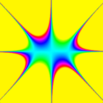
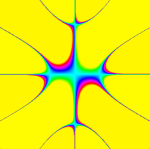
All the figures of vector fields were obtained using the visualization techniques presented in [5]. In particular, the streamlines of ${\mathfrak{Re}\left(X\right)}$ are represented as the borders of the strip flows (represented as bands of the same color) or, in particular cases that need to be emphasised, as individual trajectories. See §6.2 of the same reference for further explanation of the numerical behaviour at zeros, poles and essential singularities.

Proof of Lemma 2.5.

Let $X\in{\mathscr{E}}(s,r,d)$ be a singular complex analytic vector field. It follows immediately, from (4), that $T^{*}X=X$ for some non–trivial $T\in Aut({\mathbb{C}})$ if and only if

1. ${\tt a}^{d}={\tt a}^{s-r-1}=1$, and

2. all three sets ${\mathcal{Z}}$, ${\mathcal{P}}$ and ${\mathcal{E}}$ are $T$–symmetric.

Note that condition (a) is equivalent to ${\tt a}={\text{\myfont e}}^{i2\pi/{\tt k}}$, with ${\tt k}\in\mathscr{D}\backslash\{1\}$, $\mathscr{D}$ as in (5). So $T(w)={\text{\myfont e}}^{i2\pi j/{\tt k}}w+{\tt b}$ for $j=1,\ldots,{\tt k}$ and ${\tt b}\in{\mathbb{C}}$ as above.

Since all of $s,r,d<\infty$, condition (b) implies that $T$ can not be a parabolic transformation; i.e. $T$ has two distinct fixed points in ${\widehat{\mathbb{C}}}$. One of them is $\infty$, so if ${\tt b}\neq 0$ then ${\tt k}\neq 1$, which in turn implies that $T$ is a non–trivial rotation with center $C$. ∎

In particular, if ${\tt k}=\gcd(d,s-r-1)=1$ then $Aut({\mathbb{C}})_{X}=\{id\}$.

As is usual the triviality of the isotropy group of $X\in{\mathscr{E}}(s,r,d)$ has geometric implications on the quotient spaces.

Remark 2.11.

From the description (4) of the action $\mathcal{A}$, of $Aut({\mathbb{C}})$ on ${\mathscr{E}}(s,r,d)_{id}$ in terms of the divisor of $X$, it is clear that for $s+r+d\geq 2$, $\mathcal{A}$ is a proper map.

It is well known, see for instance [16] pp. 53, that the quotient ${\mathscr{E}}(s,r,d)_{id}/Aut({\mathbb{C}})$ is a manifold of dimension $dim({\mathscr{E}}(s,r,d)_{id})-dim(Aut({\mathbb{C}}))$. Naturally ${\mathscr{E}}(s,r,d)_{id}$ is open and dense in ${\mathscr{E}}(s,r,d)$, thus $dim({\mathscr{E}}(s,r,d)_{id})=dim({\mathscr{E}}(s,r,d))$. The analogous fact holds for the action of $Aut({\mathbb{C}})\times\mathbb{S}^{1}$.

From this it follows that both

$$\pi_{1}:{\mathscr{E}}(s,r,d)_{id}\longrightarrow\frac{{\mathscr{E}}(s,r,d)_{id}}{Aut({\mathbb{C}})}\text{ \ \ and \ \ }(\pi_{2}\circ\pi_{1}):{\mathscr{E}}(s,r,d)_{id}\longrightarrow\frac{{\mathscr{E}}(s,r,d)_{id}}{Aut({\mathbb{C}})\times\mathbb{S}^{1}},$$

in (2), are holomorphic and real–analytic principal $Aut({\mathbb{C}})$ and $(Aut({\mathbb{C}})\times\mathbb{S}^{1})$–bundles, respectively.

Lemma 2.12.

Let $s+r+d\geq 2$ and $d\geq 1$, then ${\mathscr{E}}(s,r,d)_{id}$ is a holomorphic trivial principal $Aut({\mathbb{C}})$–bundle.

When $d=0$ the isotropy group $Aut({\mathbb{C}})_{X}$ for $X\in{\mathscr{E}}(s,r,0)$ does not generically fix $\infty\in{\widehat{\mathbb{C}}}$, see §4.3 for further details.

Proof.

On ${\mathscr{E}}(s,r,d)_{id}$, every fiber is a copy of $Aut({\mathbb{C}})$. We shall explicitly exhibit three choices of global sections. We start by recalling that $X\in{\mathscr{E}}(s,r,d)$ can be expressed as

$$X(z)=\lambda\ \frac{z^{s}+a_{1}z^{s-1}+a_{2}z^{s-2}+\ldots+a_{s}}{z^{r}+b_{1}z^{r-1}+b_{2}z^{r-2}+\ldots+b_{r}}\exp\big{(}c_{0}z^{d}+c_{1}z^{d-1}+c_{2}z^{d-2}+\ldots+c_{d-1}z\big{)}\ \frac{\partial}{\partial z},$$

since the coefficient $c_{d}$ can be incorporated in $\lambda$.

Next we consider a “gauge transformation prospect”

$$\begin{array}[]{ccl}\mathcal{G}:\frac{{\mathscr{E}}(s,r,d)_{id}}{Aut({\mathbb{C}})}&\longrightarrow&Aut({\mathbb{C}})\\ {[X]}&\longmapsto&G(w)={\tt a}w+{\tt b},\end{array}$$

with suitable ${\tt a}$ and ${\tt b}$ that will depend on the specific representative $X$ of the class $[X]$. We shall now procede to choose appropiate ${\tt a}$ and ${\tt b}$.

$\bullet$ The choice ${\tt a}=\big{(}\frac{1}{c_{0}}\big{)}^{1/d}$, forces the polynomial that appears in the exponential of the expression for $(G^{*}X)(w)$ to be monic.

$\bullet$ Recalling that the barycenters of ${\mathcal{Z}}$, ${\mathcal{P}}$ and ${\mathcal{E}}$ are ${\tt Z}=-a_{1}/s$, ${\tt P}=-b_{1}/r$ and ${\tt E}=-c_{1}/(dc_{0})$ respectively, we shall choose ${\tt b}$ such that one of the polynomials appearing in the expression for $(G^{*}X)(w)$ is centered.

This provides us with the following three explicit global sections:

1. $d\geq 2$: In this case, given $[X]\in\frac{{\mathscr{E}}(s,r,d)_{id}}{Aut({\mathbb{C}})}$, choose ${\tt b}=-\frac{c_{1}}{dc_{0}}={\tt E}$ (so $G^{-1}({\tt E})=0$); we then obtain the global section

   (6) $$\begin{array}[]{ccl}\sigma:\frac{{\mathscr{E}}(s,r,d)_{id}}{Aut({\mathbb{C}})}&\longrightarrow&{\mathscr{E}}(s,r,d)_{id}\\ {[X]}&\longmapsto&(G^{*}X)(w)=\widetilde{\lambda}\ \frac{w^{s}+\widetilde{a}_{1}w^{s-1}+\widetilde{a}_{2}w^{s-2}+\ldots+\widetilde{a}_{s}}{w^{r}+\widetilde{b}_{1}w^{r-1}+\widetilde{b}_{2}w^{r-2}+\ldots+\widetilde{b}_{r}}\hfill\\ &&\hskip 72.0pt\exp\big{(}w^{d}+\widetilde{c}_{2}w^{d-2}+\ldots+\widetilde{c}_{d-1}w\big{)}\ \frac{\partial}{\partial w}.\end{array}$$

   That is, all three polynomials are monic and the one appearing in the exponential of the expression for $(G^{*}X)(w)$ is centered.

   A special case is when ${\mathcal{Z}}={\mathcal{P}}=\varnothing$ and $d\geq 2$,

   $(G^{*}X)(w)=\widetilde{\lambda}\exp(w^{d}+\widetilde{c}_{2}w^{d-2}+\ldots+\widetilde{c}_{d-1}w)\frac{\partial}{\partial w}$.

   Compare with §8.6 of [4].

2. $s\geq 1$: In this case, given $[X]\in\frac{{\mathscr{E}}(s,r,d)_{id}}{Aut({\mathbb{C}})}$, choose ${\tt b}=-\frac{a_{1}}{s}={\tt Z}$ (so $G^{-1}({\tt Z})=0$); we then obtain the global section

   (7) $$\begin{array}[]{ccl}\sigma:\frac{{\mathscr{E}}(s,r,d)_{id}}{Aut({\mathbb{C}})}&\longrightarrow&{\mathscr{E}}(s,r,d)_{id}\\ {[X]}&\longmapsto&(G^{*}X)(w)=\widetilde{\lambda}\ \frac{w^{s}+\widetilde{a}_{2}w^{s-2}+\ldots+\widetilde{a}_{s}}{w^{r}+\widetilde{b}_{1}w^{r-1}+\ldots+\widetilde{b}_{r}}\hfill\\ &&\hskip 63.0pt\exp\big{(}w^{d}+\widetilde{c}_{1}w^{d-1}+\ldots+\widetilde{c}_{d-1}w\big{)}\ \frac{\partial}{\partial w}.\end{array}$$

   That is, all three polynomials are monic and the one corresponding to the zeros of $(G^{*}X)(w)$ is centered.

3. $r\geq 1$: In this case, given $[X]\in\frac{{\mathscr{E}}(s,r,d)_{id}}{Aut({\mathbb{C}})}$, choose ${\tt b}=-\frac{b_{1}}{s}={\tt P}$ (so $G^{-1}({\tt P})=0$); we then obtain the global section

   (8) $$\begin{array}[]{ccl}\sigma:\frac{{\mathscr{E}}(s,r,d)_{id}}{Aut({\mathbb{C}})}&\longrightarrow&{\mathscr{E}}(s,r,d)_{id}\\ {[X]}&\longmapsto&(G^{*}X)(w)=\widetilde{\lambda}\ \frac{w^{s}+\widetilde{a}_{1}w^{s-1}+\ldots+\widetilde{a}_{s}}{w^{r}+\widetilde{b}_{2}w^{r-2}+\ldots+\widetilde{b}_{r}}\hfill\\ &&\hskip 63.0pt\exp\big{(}w^{d}+\widetilde{c}_{1}w^{d-1}+\ldots+\widetilde{c}_{d-1}w\big{)}\ \frac{\partial}{\partial w}.\end{array}$$

   That is, all three polynomials are monic and the one corresponding to the poles of $(G^{*}X)(w)$ is centered.

Finally, note that any $(s,r,d)$ such that ${\mathscr{E}}(s,r,d)_{id}$ is an $Aut({\mathbb{C}})$–bundle falls in one of the above cases. ∎

Remark 2.13.

Recalling that $\mathbb{S}^{1}$ acts by ${\text{\myfont e}}^{i\theta}:X\longmapsto{\text{\myfont e}}^{i\theta}X$ and preserves the singular flat metric $g_{X}$; the normal forms given by (6), (7) and (8) can be extended to consider the action of $Aut({\mathbb{C}})\times\mathbb{S}^{1}$ by requiring that $\widetilde{\lambda}\in{\mathbb{R}}^{+}$. This then produces the desired vector field $X$ and $({\widehat{\mathbb{C}}},g_{X})$ in normal form.

In order to finish the proof of the Main Theorem, we still need to show the arithmetic condition “${\tt k}\not|q$ and ${\tt k}\not|r$, for all non–trivial common divisors ${\tt k}$ of $d$ and $(s-r-1)$ implies that ${\mathscr{E}}(s,r,d)={\mathscr{E}}(s,r,d)_{id}$”.

2.3. Obstructions for the existence of non–trivial symmetries

The purpose of this section is to characterize those vector fields $X\in{\mathscr{E}}(s,r,d)$ that have non–trivial isotropy group $Aut({\mathbb{C}})_{X}\cong{\mathbb{Z}}_{\tt k}$, for ${\tt k}\in\mathscr{D}\backslash\{1\}$, recall (5).

From Corollary 2.6 we see that there are two obstructions for the existence of $X\in{\mathscr{E}}(s,r,d)$ with $Aut({\mathbb{C}})_{X}\neq\{id\}$.

With this in mind we shall start by considering the partition of ${\mathcal{Z}}$, ${\mathcal{P}}$ and ${\mathcal{E}}$ into orbits under the action of $Aut({\mathbb{C}})_{X}$.

Remark 2.14 (Orbit structure).

Recalling that $C$ is the fixed point of the discrete rotation group $\Gamma$, it is evident that:

The configurations ${\mathcal{Z}}$, ${\mathcal{P}}$ and ${\mathcal{E}}$ are $Aut({\mathbb{C}})_{X}$–symmetric if and only if each configuration ${\mathcal{Z}}$, ${\mathcal{P}}$ and ${\mathcal{E}}$ is evenly distributed on circles (of any given radius $R\geq 0$) centered about the fixed point $C$, generically on more than one circle.

Moreover, as will be shown, $C\in{\mathcal{Z}}\cup{\mathcal{P}}$.

From (4), it is clear that the set of poles and zeros of $X$ do not intersect, that is ${\mathcal{Z}}\cap{\mathcal{P}}=\varnothing$; however ${\mathcal{E}}$ is unrelated to ${\mathcal{Z}}$ and ${\mathcal{P}}$, in the sense that ${\mathcal{E}}\cap{\mathcal{Z}}$ and ${\mathcal{E}}\cap{\mathcal{P}}$ may be non–empty.

Assuming $\gcd(d,s-r-1)\neq 1$ let $X\in{\mathscr{E}}(s,r,d)\backslash{\mathscr{E}}(s,r,d)_{id}$.

The search for an alternative for Lemma 2.5 is expressed as (A), (B) and (C) below.

1. Choose ${\tt k}\in\mathscr{D}\backslash\{1\}$ and let it remain fixed.

2. For the $d$ roots ${\mathcal{E}}$ of the polynomial $E(z)$, recall the orbit structure of Remark 2.14 and proceed as follows:

   1. Consider the partitions of $d$ as a sum of positive integers, say

      $$Part(d)=\left\{\{d_{\iota,\kappa}\}_{\iota=1}^{\ell_{\kappa}}\Big{|}\ d=\sum\limits_{\iota=1}^{\ell_{\kappa}}d_{\iota,\kappa},\kappa=1,\ldots,p(d)\right\},$$

      where $p(d)$ is the partition function of $d$ (the number of possible integer partitions of $d$).

   2. Let $\{d_{\iota,\kappa}\}_{\iota=1}^{\ell_{\kappa}}$ be a partition such that $d_{j,\kappa}={\tt k}\nu_{j}$, for some $\nu_{j}\in{\mathbb{N}}$, say

      $$d=d_{1,\kappa}+d_{2,\kappa}+\ldots+\underbrace{d_{j,\kappa}}_{\ \,={\tt k}\nu_{j}}+\ldots+d_{\ell_{\kappa},\kappa},$$

      choose this partition and place ${\tt k}$ equally spaced roots on a circle $L_{j}$ centered about $C$ of a chosen radius $R_{j}>0$, all with the same multiplicity $\nu_{j}$.

   3. If there are still some $d_{\iota,\kappa}={\tt k}\nu_{\iota}$, for $\nu_{\iota}\in{\mathbb{N}}$ in the same partition, place ${\tt k}$ equally spaced roots on a circle $L_{i}$ centered about $C$ (possibly the same circle as before but the roots are to be placed on different positions), once again each root with multiplicity $\nu_{\iota}$. Repeat (B)iii) if possible or proceed to (B)iv) below.

   4. Finally, place the rest of the roots at $C$; hence $C$ will be a root of $E(z)$ of multiplicity equal to $d$ minus the number of roots (counted with multiplicity) already placed on circles of positive radius.

3. For the placement of the poles and zeros of $X$, we proceed as in (B) replacing “$d$” and “roots of $E(z)$” with “$r$” and “roots of $P(z)$”, and “$s$” and “roots of $Q(z)$”, respectively.
   However since ${\tt k}|(s-r-1)$, then ${\tt k}|s$ and ${\tt k}|r$ can not occur simultaneously; leaving the following cases.

   1. ${\tt k}\not|s$ and ${\tt k}\not|r$.

   2. ${\tt k}|s$ and ${\tt k}\not|r$.

   3. ${\tt k}\not|s$ and ${\tt k}|r$.

   Case (C)a) can not occur: if ${\tt k}\not|s$ then we must place a zero of $X$ at the fixed point $C$ of the rotation (by considering the partitions of $s$ as a sum of positive integers as in (B), it follows from the orbit structure, i.e. Remark 2.14, that at least one zero of $X$ must be placed at $C$). Similarly if ${\tt k}\not|r$ then we must place a pole of $X$ at the fixed point $C$ of the rotation; but ${\mathcal{Z}}\cap{\mathcal{P}}=\varnothing$.

   Case (C)b) requires a pole of $X$ at the fixed point $C$ and case (C)c) requires a zero of $X$ at the fixed point $C$. Thus either (C)b) or (C)c) occurs, but not both.

The arithmetic conditions stated as cases (b) and (c) above can be interpreted geometrically as $C$ has to be either a pole or a zero of $X$, respectively. However, since $X$ have non–trivial isotropy group, then there are local restrictions on the allowed multiplicity $\nu$ of $C$.

Consider the phase portrait in a neighborhood of the center of rotation $C\in{\mathbb{C}}$. This together with the fact that the non–trivial isotropy groups are the discrete rotation groups ${\mathbb{Z}}_{\tt k}$ with ${\tt k}\in\mathscr{D}\backslash\{1\}$, implies that:

1. When $C$ is a pole of $X$ of multiplicity $\nu$, the phase portrait of $X$ in a neighborhood of $C$ consists of $2(\nu+1)$ hyperbolic sectors. Since hyperbolic sectors come in pairs, ${\tt k}|(\nu+1)$ is required.

2. On the other hand, when $C$ is a zero of $X$ of multiplicity $\nu$, the phase portrait of $X$ in a neighborhood of $C$ consists of $2(\nu-1)$ elliptic sectors. Since elliptic sectors come in pairs, ${\tt k}|(\nu-1)$ is required.

With this in mind we can now restate Lemma 2.5.

Theorem 2.15.

Let $X\in{\mathscr{E}}(s,r,d)$. The discrete rotation group

$\Gamma=\left\{T(w)={\text{\myfont e}}^{i2\pi j/{\tt k}}w+{\tt b},j=1,\ldots,{\tt k}\right\}$ $\cong{\mathbb{Z}}_{\tt k}$, ${\tt k}\geq 2$, ${\tt b}\in{\mathbb{C}}$

leaves invariant $X$ if and only if

1. ${\tt k}$ is a common divisor of $d$ and $(s-r-1)$,

2. either

   1. (${\tt k}|s$ and ${\tt k}\not|r$): $C$ is a pole of $X$ of multiplicity $\nu\geq 1$ with ${\tt k}|(\nu+1)$; furthermore the rest of the poles and all the zeros are evenly distributed on circles centered about $C$, thus $r={\tt k}k_{r}+\nu$ with ${\tt k}\not|\nu$ and $s={\tt k}k_{s}$,

      or

   2. (${\tt k}\not|s$ and ${\tt k}|r$): $C$ is a zero of $X$ of multiplicity $\nu\geq 1$ with ${\tt k}|(\nu-1)$; furthermore the rest of the zeros and all the poles are evenly distributed on circles centered about $C$, thus $s={\tt k}k_{s}+\nu$ with ${\tt k}\not|\nu$ and $r={\tt k}k_{r}$,

3. ${\mathcal{E}}$ is evenly distributed on circles centered about $C$, thus $d={\tt k}k_{d}$.

Otherwise $Aut({\mathbb{C}})_{X}=\{id\}$.

Proof.

Condition (1) is a restatement of (1) of Lemma 2.5. The discussion previous to the statement of Theorem 2.15 together with (4) are enough to show that conditions (2) and (3) are equivalent to (2) of Lemma 2.5. ∎

Remark 2.16.

1. Theorem 2.15 provides a way of realizing those $X\in{\mathscr{E}}(s,r,d)$ that are $\Gamma$–symmetric for $\Gamma\cong{\mathbb{Z}}_{\tt k}$, ${\tt k}\in\mathscr{D}\backslash\{1\}$. See §3.1 for the explicit construction.

2. Note that the divisibility conditions on the multiplicity $\nu$ of the pole or zero at the fixed point $C$ are automatically satisfied.

That is, if (1), (3) and (${\tt k}|s$ and ${\tt k}\not|r$) are satisfied, then $r={\tt k}k_{r}+\nu$ for some $\nu\geq 1$ with ${\tt k}\not|\nu$ and ${\tt k}|(\nu+1)$.

Similarly, if (1), (3) and (${\tt k}\not|s$ and ${\tt k}|r$) are satisfied, then $s={\tt k}k_{s}+\nu$ for some $\nu\geq 1$ with ${\tt k}\not|\nu$ and ${\tt k}|(\nu-1)$.

Both statements follow from (4).

As an immediate consequence of Theorem 2.15 we have:

Corollary 2.17.

$Aut({\mathbb{C}})_{X}=\{id\}$ if and only if
$\bullet\ \gcd(d,s-r-1)=1$, or
$\bullet\ {\tt k}\not|s$ and ${\tt k}\not|r$, for all non–trivial common divisors ${\tt k}$ of $d$ and $(s-r-1)$. ∎

Which in turn finishes the proof of the Main Theorem.

Note that as stated in (1) of the Main Theorem, even if $\gcd(d,s-r-1)\neq 1$ it is possible that ${\mathscr{E}}(s,r,d)={\mathscr{E}}(s,r,d)_{id}$, as the next example shows.

Example 2.18 ($\gcd(d,s-r-1)\neq 1$ does not guarantee the existence of $X$ with non–trivial symmetry).

Let $s=11$, $r=7$ and $d=6$, then $\gcd(d,s-r-1)=\gcd(6,3)=3\neq 1$. However $3\not|11$ and $3\not|7$. Thus by Corollary 2.17, ${\mathscr{E}}(11,7,6)={\mathscr{E}}(11,7,6)_{id}$.

On the other hand for ${\mathscr{E}}(s,r,d)={\mathscr{E}}(s,r,d)_{id}$ we must check that the condition “${\tt k}\not|s$ and ${\tt k}\not|r$”, is satisfied for all non–trivial common divisors ${\tt k}$ of $d$ and $(s-r-1)$.

Example 2.19 (Not all common divisors of $d$ and $s-r-1$ give rise to symmetry).

Let $s=35$, $r=4$ and $d=30$, then $\gcd(d,s-r-1)=\gcd(30,30)=30\neq 1$. Moreover $\mathscr{D}=\{1,2,3,5,6,10,15,30\}$ and we see that

$$2|35 \text{ and }2\not|4 3\not|35 \text{ and }3\not|4 5\not|35 \text{ and }5|4$$

$$6\not|35 \text{ and }6\not|4 10\not|35 \text{ and }10\not|4 15\not|35 \text{ and }15\not|4$$

$$30\not|35 \text{ and }30\not|4.$$

It follows, from Theorem 2.15, that only ${\mathbb{Z}}_{\it k}$ with ${\it k}=2,5$ can be non–trivial symmetry groups for $X\in{\mathscr{E}}(35,4,30)$. In fact

$$X_{2}(z)=\frac{z^{35}}{z^{4}-1}{\text{\myfont e}}^{z^{30}}\frac{\partial}{\partial z},\quad X_{5}(z)=\frac{(z^{5}-1)^{7}}{z^{4}}{\text{\myfont e}}^{z^{30}}\frac{\partial}{\partial z}\in{\mathscr{E}}(35,4,30)$$

are ${\mathbb{Z}}_{2}$–invariant and ${\mathbb{Z}}_{5}$–invariant, respectively. So ${\mathscr{E}}(35,4,30)\neq{\mathscr{E}}(35,4,30)_{id}$.

We point out some relevant particular cases.

Remark 2.20.

1. The special case ${\mathscr{E}}(0,0,d)={\mathscr{E}}(0,0,d)_{id}$ since $s=r=0$ so $\gcd(d,-1)=1$. See also theorem 8.16 in [4].

2. For each $d\geq 2$ there are $X\in{\mathscr{E}}(0,d-1,d)$ such that $Aut({\mathbb{C}})_{X}={\mathbb{Z}}_{d}$. Thus in fact all the cyclic groups appear as isotropy groups of $X\in{\mathscr{E}}(0,r,d)$ for appropriate pairs $(r,d)$.

3. For each sufficiently large pair $(r,d)$ with $\gcd(d,r+1)\neq 1$, there are an infinite number of non conformally equivalent configurations of the roots ${\mathcal{E}}$ of $E(z)$ and ${\mathcal{P}}$ of $P(z)$ which are invariant by the non–trivial $T\in Aut({\mathbb{C}})_{X}\neq\{id\}$. This follows from Remark 2.14 and the fact that the quotient of the radii of an annulus is a conformal invariant; thus there are an infinite number of possible configurations of the roots ${\mathcal{E}}$ and ${\mathcal{P}}$.

This last special case can be re–stated as:

Corollary 2.21.

For each sufficiently large pair $(r,d)$ with ${\tt k}=\gcd(d,r+1)\neq 1$, there are an infinite number of non conformally equivalent $X\in{\mathscr{E}}(0,r,d)$ with isotropy group $Aut({\mathbb{C}})_{X}\cong{\mathbb{Z}}_{\tt k}$.

3. Normal forms for ${\mathscr{E}}(s,r,d)$

We start with a formal definition.

Definition 3.1.

A normal form of $X\in{\mathscr{E}}(s,r,d)$ is a representative of its class under the pullback action $\mathcal{A}$ of $Aut({\mathbb{C}})$.

The explicitness of the global sections, Lemma 2.12, immediately provides us with.

Corollary 3.2 (Normal forms for ${\mathscr{E}}(s,r,d)_{id}$).

For $s+r+d\geq 2$ and $d\geq 1$, global normal forms for $X\in{\mathscr{E}}(s,r,d)_{id}$ are given by $(G^{*}X)(w)$ as in (6), (7) and (8). ∎

Remark 3.3.

The term global refers to the fact that the expressions for $(G^{*}X)(w)$ given by (6), (7) and (8) are valid for every $X\in{\mathscr{E}}(s,r,d)_{id}$ and also throughout ${\widehat{\mathbb{C}}}$.

Furthermore, an application of Theorem 2.15 enables us to also find the normal forms for $X\in{\mathscr{E}}(s,r,d)$ with non–trivial isotropy.

3.1. Realizing $X\in{\mathscr{E}}(s,r,d)$ with non–trivial isotropy group

We proceed as follows:

1) $d$ and $(s-r-1)$ must have non–trivial divisors ${\tt k}\in\mathscr{D}\backslash\{1\}$.

Given $\Gamma\cong{\mathbb{Z}}_{\tt k}$ a discrete rotation group, $X\in{\mathscr{E}}(s,r,d)$ is $\Gamma$–symmetric if and only if the following two conditions occur:

2) The configuration of poles ${\mathcal{P}}$ and zeros ${\mathcal{Z}}$ of $X$ are $\Gamma$–symmetric and either

1. $X$ has a pole as a fixed point of $\Gamma$, of multiplicity $\nu$ with ${\tt k}|(\nu+1)$, or

2. $X$ has a zero as a fixed point of $\Gamma$, of multiplicity $\nu$ with ${\tt k}|(\nu-1)$.

3) The configuration ${\mathcal{E}}$ of roots of $E(z)$ are $\Gamma$–symmetric.

3.1.1. Zeros and poles with arbitrary multiplicity

With the above in mind we immediately obtain.

Theorem 3.4 (Realizing vector fields with non–trivial symmetry).

Consider ${\mathscr{E}}(s,r,d)$ with $\mathscr{D}\backslash\{1\}\neq\varnothing$. The discrete rotation group

$\Gamma=\left\{T(w)={\text{\myfont e}}^{i2\pi j/{\tt k}}w+{\tt b},j=1,\ldots,{\tt k}\right\}$ $\cong{\mathbb{Z}}_{\tt k}$, ${\tt k}\in\mathscr{D}\backslash\{1\}$, ${\tt b}\in{\mathbb{C}}$,

with center of rotation

$C\doteq{\tt b}/(1-{\text{\myfont e}}^{i2\pi/{\tt k}})\in{\mathbb{C}}$,

leaves invariant those $X\in{\mathscr{E}}(s,r,d)$ that satisfy the following conditions.

1. (${\tt k}|s$ and ${\tt k}\not|r$): in this case $C$ is a pole, furthermore

   $$X(z)=\lambda\,\frac{\prod\limits_{j=1}^{k_{s}}\prod\limits_{\ell=1}^{\tt k}\Big{[}z-C-(r_{j}{\text{\myfont e}}^{i\theta_{j}})^{\ell/{\tt k}}\Big{]}}{(z-C)^{\nu}\prod\limits_{j=1}^{k_{r}}\prod\limits_{\ell=1}^{\tt k}\Big{[}z-C-(R_{j}{\text{\myfont e}}^{i\alpha_{j}})^{\ell/{\tt k}}\Big{]}}\exp\left\{(z-C)^{\mu}\prod\limits_{j=1}^{k_{d}}\prod\limits_{\ell=1}^{\tt k}\Big{[}z-C-(\rho_{j}{\text{\myfont e}}^{i\beta_{j}})^{\ell/{\tt k}}\Big{]}\right\}\frac{\partial}{\partial z},$$

   for choices of ${\tt k},k_{s},k_{r},k_{d}$ such that $s={\tt k}k_{s}$, $r={\tt k}k_{r}+\nu$, $d={\tt k}k_{d}+\mu$, $\{r_{j}\},\{R_{j}\},\{\rho_{j}\}\subset{\mathbb{R}}^{+}$, $\{\theta_{j}\},\{\alpha_{j}\},\{\beta_{j}\}\subset{\mathbb{R}}$, $\mu\in{\mathbb{N}}\cup\{0\}$ and $\nu\in{\mathbb{N}}$ such that ${\tt k}|(\nu+1)$.

2. (${\tt k}\not|s$ and ${\tt k}|r$): in this case $C$ is a zero, furthermore

   $$X(z)=\lambda\,\frac{(z-C)^{\nu}\prod\limits_{j=1}^{k_{s}}\prod\limits_{\ell=1}^{\tt k}\Big{[}z-C-(r_{j}{\text{\myfont e}}^{i\theta_{j}})^{\ell/{\tt k}}\Big{]}}{\prod\limits_{j=1}^{k_{r}}\prod\limits_{\ell=1}^{\tt k}\Big{[}z-C-(R_{j}{\text{\myfont e}}^{i\alpha_{j}})^{\ell/{\tt k}}\Big{]}}\exp\left\{(z-C)^{\mu}\prod\limits_{j=1}^{k_{d}}\prod\limits_{\ell=1}^{\tt k}\Big{[}z-C-(\rho_{j}{\text{\myfont e}}^{i\beta_{j}})^{\ell/s}\Big{]}\right\}\frac{\partial}{\partial z},$$

   for choices of ${\tt k},k_{s},k_{r},k_{d}$ such that $s={\tt k}k_{s}+\nu$, $r={\tt k}k_{r}$, $d={\tt k}k_{d}+\mu$, $\{r_{j}\},\{R_{j}\},\{\rho_{j}\}\subset{\mathbb{R}}^{+}$, $\{\theta_{j}\},\{\alpha_{j}\},\{\beta_{j}\}\subset{\mathbb{R}}$, $\mu\in{\mathbb{N}}\cup\{0\}$ and $\nu\in{\mathbb{N}}$ such that ${\tt k}|(\nu-1)$. ∎

Remark 3.5.

Note that the expressions in Theorem 3.4 are in fact normal forms for $X\in{\mathscr{E}}(s,r,d)\backslash{\mathscr{E}}(s,r,d)_{id}$.

3.1.2. Simple zeros and simple poles in ${\mathbb{C}}$

The case of $X$ having simple poles and simple zeros has further structure. Let

${\mathscr{E}}(s,r,d)^{S}:=\{X\in{\mathscr{E}}(s,r,d)\ |\ \text{all the poles and zeros of }X\text{ in }{\mathbb{C}}\text{ are simple}\}$.

From the orbit structure (Remark 2.14), Theorem 2.15 and the fact that only simple poles and zeros are allowed, it follows that $s={\tt k}k_{s}+1$ or $r={\tt k}k_{r}+1$, with $k_{s},k_{r}\in{\mathbb{N}}\cup\{0\}$.

Let us first consider the case $r={\tt k}k_{r}+1$ with $k_{r}\geq 0$. Then if we want $X\in{\mathscr{E}}(s,r,d)^{S}$ to have non–trivial isotropy group, we must require that $s={\tt k}k_{s}$, with $k_{s}\geq 0$. On the other hand ${\tt k}|(s-r-1)=((k_{s}-k_{r}){\tt k}-2)$ hence ${\tt k}=2$ and $d=2k_{d}$ for $k_{d}\geq 1$. We have then proved.

Proposition 3.6.

Let $X\in{\mathscr{E}}(s,r,d)^{S}$ have non–trivial isotropy group fixing a pole of $X$. Then $r=2k_{r}+1$ for $k_{r}\in{\mathbb{N}}\cup\{0\}$, $Aut({\mathbb{C}})_{X}\cong{\mathbb{Z}}_{2}$ and the vector fields $X$ are of the form

$$X(z)=\lambda\,\frac{\prod\limits_{j=1}^{k_{s}}\Big{[}(z-C)^{2}-q_{j}^{2}\Big{]}}{(z-C)\prod\limits_{j=1}^{k_{r}}\Big{[}(z-C)^{2}-p_{j}^{2}\Big{]}}\exp\left\{(z-C)^{2\mu}\prod\limits_{j=1}^{k^{\prime}_{d}}\Big{[}(z-C)^{2}-e_{j}^{2}\Big{]}\right\}\frac{\partial}{\partial z},$$

where $k_{r}=\frac{r-1}{2}\geq 0$, $k_{s}=\frac{s}{2}\geq 0$, $\mu\geq 0$, $k^{\prime}_{d}=\frac{d-2\mu}{2}\geq 0$, all the $\{p_{j}\}\subset{\mathbb{C}}\backslash\{0\}$ and $\{q_{j}\}\subset{\mathbb{C}}\backslash\{0\}$ are distinct, and the $\{e_{j}\}\subset{\mathbb{C}}$ need not be distinct. ∎

Example 3.7.

Let

$$X(z)=\frac{{\text{\myfont e}}^{z^{2}}}{z(z^{2}+1)}\frac{\partial}{\partial z}\in{\mathscr{E}}(0,3,2)^{S}.$$

Its isotropy group is $Aut({\mathbb{C}})_{X}={\mathbb{Z}}_{2}$, see Figure 3 (c).

However the case $s={\tt k}k_{s}+1$ with $k_{s}\geq 0$ is different. In this case, upon a similar examination we have.

Proposition 3.8.

For each ${\tt k}\geq 2$, let $s={\tt k}k_{s}+1\geq 1$, $r={\tt k}k_{r}\geq 0$ and $d={\tt k}k_{d}\geq 1$ for $k_{s},k_{r},k_{d}\in{\mathbb{N}}\cup\{0\}$. Then there is an $X\in{\mathscr{E}}(s,r,d)^{S}$ with non–trivial isotropy group $Aut({\mathbb{C}})_{X}\cong{\mathbb{Z}}_{s}$ fixing a zero of $X$.

These vector fields $X$ are of the form

$$X(z)=\lambda\,\frac{(z-C)\prod\limits_{j=1}^{k_{s}}\prod\limits_{\ell=1}^{\tt k}\Big{[}z-C-(r_{j}{\text{\myfont e}}^{i\theta_{j}})^{\ell/{\tt k}}\Big{]}}{\prod\limits_{j=1}^{k_{r}}\prod\limits_{\ell=1}^{\tt k}\Big{[}z-C-(R_{j}{\text{\myfont e}}^{i\alpha_{j}})^{\ell/{\tt k}}\Big{]}}\exp\left\{(z-C)^{\mu}\prod\limits_{j=1}^{k_{d}}\prod\limits_{\ell=1}^{\tt k}\Big{[}z-C-(\rho_{j}{\text{\myfont e}}^{i\beta_{j}})^{\ell/{\tt k}}\Big{]}\right\}\frac{\partial}{\partial z},$$

for choices of $\{r_{j}\},\{R_{j}\},\{\rho_{j}\}\subset{\mathbb{R}}^{+}$, $\{\theta_{j}\},\{\alpha_{j}\},\{\beta_{j}\}\subset{\mathbb{R}}$ and $\mu\in{\mathbb{N}}\cup\{0\}$ such that $\{(r_{j}{\text{\myfont e}}^{i\theta_{j}})^{\ell/{\tt k}}\}$ and $\{(R_{j}{\text{\myfont e}}^{i\alpha_{j}})^{\ell/{\tt k}}\}$ are distinct, but the $\{(\rho_{j}{\text{\myfont e}}^{i\beta_{j}})^{\ell/{\tt k}}\}$ need not necessarily be distinct. ∎

Remark 3.9 (Simple poles and zeros).

Proposition 3.6 and Proposition 3.8 can be summarized as:

1. If there is a (simple) pole of $X$ at the fixed point $C\in{\mathbb{C}}$, then the number of (simple) zeros of $X$ is even, the number of (simple) poles of $X$ is odd and the number of roots (counted with multiplicity) of the polynomial in the exponential, is even.

2. If there is a (simple) zero of $X$ at the fixed point $C\in{\mathbb{C}}$, there is no restriction other than those given by the orbit structure (Remark 2.14).

4. Singular complex analytic dictionary and $\Gamma$–symmetry

4.1. The dictionary

Previously, the authors presented a dictionary/correspondence in the complex analytic framework, which is stated below as Proposition 4.1, in particular it applies to $X$ (and $\Psi_{X}$) in the family ${\mathscr{E}}(s,r,d)$. A complete proof can be found in [4] §2.2 with further discussion in [5].

Proposition 4.1 (Singular complex analytic dictionary).

On any (non necessarily compact) Riemann surface $M$ there is a canonical one to one correspondence between:

1. Singular complex analytic vector fields $X$.

2. Singular complex analytic differential forms $\omega_{X}$, satisfying $\omega_{X}(X)\equiv 1$.

3. Singular complex analytic orientable quadratic differentials $\omega_{X}\otimes\omega_{X}$.

4. Singular flat metrics $(M,g_{X})$ with suitable singularities, trivial holonomy and provided with a real geodesic vector field ${\mathfrak{Re}\left(X\right)}$, arising from $\omega_{X}\otimes\omega_{X}$ satisfying $g_{X}({\mathfrak{Re}\left(X\right)},{\mathfrak{Re}\left(X\right)})\equiv 1$ and $g_{X}({\mathfrak{Re}\left(X\right)},{\mathfrak{Im}\left(X\right)})\equiv 0$.

5. Global singular complex analytic (possibly multivalued) distinguished parameters
   

   $\Psi_{X}(z)=\int^{z}\omega_{X}:M\longrightarrow{\widehat{\mathbb{C}}}_{t}.$

6. Pairs $\big{(}{\mathcal{R}}_{X},\pi^{*}_{X,2}(\frac{\partial}{\partial t})\big{)}$ consisting of branched Riemann surfaces ${\mathcal{R}}_{X}$, associated to the maps $\Psi_{X}$, and the vector fields $\pi^{*}_{X,2}(\frac{\partial}{\partial t})$ under the projection $\pi_{X,2}:{\mathcal{R}}_{X}\longrightarrow{\widehat{\mathbb{C}}}_{t}$. ∎

To better understand the dictionary, note that: The singular set of $X$, $Sing(X)$, is composed of zeros, poles, essential singularities and accumulation points of the above. The adjectives “singular complex analytic” should be clear for each of the objects in Proposition 4.1. The singular flat metric $g_{X}$ with singular set $Sing(X)$ is the flat Riemannian metric on $M\backslash Sing(X)$ defined as the pullback under

$\Psi_{X}:(M,g_{X})\rightarrow({\mathbb{C}}_{t},|dt|)$,

where $|dt|$ is the usual flat Riemannina metric on ${\mathbb{C}}_{t}$, see [28], [27] and [4]. The topology of the phase portrait of ${\mathfrak{Re}\left(X\right)}$ and the geometry of $g_{X}$ are subjects of current interest, some pioneering sources can be found in [4] at §1, pp. 133, §5 pp. 159 and table 2. See [5] for visualizational aspects. Applications of geometric structures associated to flat metrics $({\widehat{\mathbb{C}}},g_{X})$ can be found in [19].

The graph of $\Psi_{X}$

$${\mathcal{R}}_{X}=\{(z,t)\ |\ t=\Psi_{X}(z)\}\subset M\times{\widehat{\mathbb{C}}}_{t}$$

is a Riemann surface provided with the vector field induced by $\big{(}{\widehat{\mathbb{C}}},\frac{\partial}{\partial t}\big{)}$ via the projection of $\pi_{X,2}$, say $\big{(}{\mathcal{R}}_{X},\pi_{X,2}^{*}(\frac{\partial}{\partial t})\big{)}$.

Moreover the singular flat metric from this pair coincides with $g_{X}=\Psi_{X}^{*}|dt|$ since $\pi_{X,1}$ is an isometry (the isometry is to be understood on the complement of the corresponding singular set in ${\mathcal{R}}_{X}$). We summarize all this in the diagram

In the presence of non–trivial symmetries we have.

Theorem 4.2 (The dictionary under $\Gamma$–symmetry).

Let $\Gamma$ be a subgroup of the complex automorphisms $Aut(M)$ having quotient $proj:M\longrightarrow M/\Gamma$ to a Riemann surface.

1. On $M$ there is a canonical one to one correspondence between:

   1. $\Gamma$–symmetric singular complex analytic vector fields $X$.

   2. $\Gamma$–symmetric singular complex analytic differential forms $\omega_{X}$, satisfying $\omega_{X}(X)\equiv 1$.

   3. $\Gamma$–symmetric singular complex analytic orientable quadratic differentials $\omega_{X}\otimes\omega_{X}$.

   4. $\Gamma$–symmetric singular flat metrics $(M,g_{X})$ with suitable singularities.

   5. $\Gamma$–symmetric global singular complex analytic (possibly multivalued) distinguished parameters $\Psi_{X}$.

   6. Pairs $\big{(}{\mathcal{R}}_{X},\pi^{*}_{X,2}(\frac{\partial}{\partial t})\big{)}$ consisting of branched Riemann surfaces ${\mathcal{R}}_{X}$, associated to the $\Gamma$–symmetric maps $\Psi_{X}$.

2. Moreover, any $X$ (resp. $\Psi_{X}$) on $M$ which is invariant by a non–trivial $\Gamma<Aut(M)$ can be recognized as a lifting of a suitable vector field $Y$ (resp. function $\Psi_{Y}$) on $M/\Gamma$, as in the following diagram

Proof.

By hypothesis $proj:M\longrightarrow M/\Gamma$ determines a connected Riemann surface as a target, thus Diagram (9) holds true both for $M$ and $M/\Gamma$.

We want to show that $proj_{*}X\doteq Y$ is a well defined vector field on $M/\Gamma$.

From a local point of view, let $({\mathbb{C}},0)$ denote local charts of $M$ where $0$ corresponds to a fixed point for some $g:M\longrightarrow M$, $g\neq id$ in $\Gamma$. Without loss of generality, we assume that $proj^{-1}(proj({\mathbb{C}},0))$ is connected in $M$.

Note that $X$ is necessarily singular at $({\mathbb{C}},0)$. The trouble is that the local behaviour of $X$ is unknown. The computation of $Y$ from the germ $\big{(}({\mathbb{C}},0),X\big{)}$ is by using geometrical arguments. The fundamental domain of

$proj:({\mathbb{C}},0)\longmapsto({\mathbb{C}},0)/\Gamma$

is an angular sector $\{0\leq arg(z)\leq 2\pi/\kappa\}\subset({\mathbb{C}},0)$, $\kappa\geq 2$. Using the singular flat metric $g_{X}$ and the frame of geodesic vector fields ${\mathfrak{Re}\left(X\right)},{\mathfrak{Im}\left(X\right)}$ on the angular sectors (recall Theorem 4.1 (4)), the value of $X$ at the borders of an angular sector coincide, hence the germ $Y$ on $proj\big{(}({\mathbb{C}},0),Y\big{)}$ is well defined.

For poles, zeros and the simplest exponential isolated singularities at $({\mathbb{C}},0)$ explicit computations are provided in Table 1, which in itself is of independent interest.

The global existence of $Y$ on $M/\Gamma$ follows by an analytic continuation argument.

Diagram (10) for vector fields follows immediately, where $proj_{*}$ and $\widetilde{proj}_{*}$ are the maps induced by $proj$ on $M$ and ${\mathcal{R}}_{X}$ respectively.

Finally, the use of the dictionary extends Diagram (10) to singular complex analytic 1–forms $\omega_{X}$ and functions $\Psi_{X}$; where $g\in\Gamma$ acts on functions as $\Psi_{X}\mapsto\Psi_{X}\circ g$. Assertions (2) and (5) are done. ∎

As a matter of record, in Table 1 the linear vector field $\lambda z\frac{\partial}{\partial z}$ has complete isotropy group ${\mathbb{C}}^{*}$; however only discrete groups are considered for Theorem 4.2. However, Table 1 makes sense globally, in the last row we use $({\widehat{\mathbb{C}}},\infty)$ as germ domain.

Table 1. Computation of $Y=proj_{*}X$ given a germ $\big{(}({\mathbb{C}},0),X\big{)}$.

On $({\mathbb{C}},0)$			on $({\widehat{\mathbb{C}}},0)/\Gamma$
normal	order	isotropy	vector	differential	quadratic
form for	$\nu\in{\mathbb{Z}}$ &	group	field	1–form	differential
a germ $X$	residue	$\Gamma$	$Y$	$\omega_{Y}$	$\omega_{Y}\otimes\omega_{Y}$
	${\tt r}\in{\mathbb{C}}$
$\frac{1}{z^{\nu}}\frac{\partial}{\partial z}$	$-\nu\leq-1$	${\mathbb{Z}}_{\tt k},$	$\frac{1}{w^{(\nu+1)/{\tt k}-1}}\frac{\partial}{\partial w}$	$w^{(\nu+1)/{\tt k}-1}dw$	$w^{2(\nu+1)/{\tt k}-2}dw^{2}$
		${\tt k}|(\nu+1)$
$\lambda z\frac{\partial}{\partial z}$	$\nu=1$	${\mathbb{C}}^{*}\triangleright{\mathbb{Z}}_{\tt k}$	$\frac{\lambda w}{\tt k}\frac{\partial}{\partial w}$	$\frac{\tt k}{\lambda w}dw$	$\frac{{\tt k}^{2}}{\lambda^{2}w^{2}}dw^{2}$
	${\tt r}=\/\lambda$
$z^{2}\frac{\partial}{\partial z}$	$\nu=2$	$id$	$w^{2}\frac{\partial}{\partial w}$	$\frac{1}{w^{2}}dw$	$\frac{1}{w^{4}}dw^{2}$
$z^{\nu}\frac{\partial}{\partial z}$	$\nu\geq 3$	${\mathbb{Z}}_{\tt k},$	$w^{(\nu-1)/{\tt k}+1}\frac{\partial}{\partial w}$	$\frac{1}{w^{(\nu-1)/{\tt k}+1}}dw$	$\frac{1}{w^{2(\nu-1)/{\tt k}+2}}dw^{2}$
	${\tt r}=0$	${\tt k}|(\nu-1)$
$\frac{z^{\nu}}{1+\lambda z^{\nu-1}}\frac{\partial}{\partial z}$	$\nu\geq 3$	$id$	$\frac{w^{\nu}}{1+\lambda w^{\nu-1}}\frac{\partial}{\partial w}$	$\frac{1+\lambda w^{\nu-1}}{w^{\nu}}dw$	$\frac{(1+\lambda w^{\nu-1})^{2}}{w^{2\nu}}dw^{2}$
	${\tt r}=\lambda\neq 0$
${\text{\myfont e}}^{z^{d}}\frac{\partial}{\partial z}$	$\nu\geq 3$	${\mathbb{Z}}_{\tt k},$	${\text{\myfont e}}^{w^{d/{\tt k}}}\frac{\partial}{\partial w}$	${\text{\myfont e}}^{-w^{d/{\tt k}}}dw$	${\text{\myfont e}}^{-w^{2d/{\tt k}}}dw^{2}$
	${\tt r}=0$	${\tt k}|d$

4.2. Description of $Y=proj_{*}X$, for $X\in{\mathscr{E}}(s,r,d)$

Recall that for $X\in{\mathscr{E}}(s,r,d)$; the rotation $\langle T_{\tt k}:z\mapsto{\text{\myfont e}}^{2\pi i/{\tt k}}z+{\tt b}\rangle$ is the generator of the isotropy group $Aut({\mathbb{C}})_{X}$, $C$ is the center of rotation of $T$ and $proj:{\widehat{\mathbb{C}}}_{z}\longrightarrow{\widehat{\mathbb{C}}}_{z}/{\mathbb{Z}}_{\tt k}={\widehat{\mathbb{C}}}_{w}$.

Proposition 4.3.

Let $X\in{\mathscr{E}}(s,r,d)$ having $Aut({\mathbb{C}})_{X}\cong{\mathbb{Z}}_{\tt k}$, ${\tt k}\geq 2$, as isotropy group. The quotient vector field  $Y=proj_{*}X$  has the following characteristics.

1. $Y\in{\mathscr{E}}(s^{\prime},r^{\prime},d^{\prime})$ has $s^{\prime}$ zeros, $r^{\prime}$ poles and an essential singularity of 1–order $d^{\prime}$ at $\infty$, where

   $\bullet\ d^{\prime}=d/{\tt k}$,

   $\bullet\ s^{\prime}=s/{\tt k}$, $r^{\prime}=\frac{r+1}{\tt k}-1$ when $C$ is a pole of $X$,

   $\bullet\ r^{\prime}=r/{\tt k}$, $s^{\prime}=\frac{s-1}{\tt k}+1$ when $C$ is a zero of $X$.

2. The isotropy of $Y$ in $Aut({\mathbb{C}})$ is trivial.

3. The phase portrait of $X$ is the pullback via $\{z\mapsto{\text{\myfont e}}^{2\pi i/{\tt k}}z+{\tt b}\}$ of the phase portrait of $Y$.

Proof.

Since $\Psi_{X}(z)=\int^{z}\omega_{X}$, the diagram (10) commutes and assertions (2) and (3) follow.

Now, we compute the nature of the singularities of $Y$.

If $d>1$, then $\infty$ is an isolated essential singularity of $X$ having $2d$ entire sectors (§5.3.1 pp. 151, figure 3 pp. 153 [4]). By theorem (A) pp. 130, Corollary 10.1 pp. 216 in [4], it follows that since $proj$ is ${\tt k}$ to 1 around $\infty$ and since ${\tt k}|d$ then the phase portrait of ${proj}_{*}(X)$ has $2d^{\prime}=d/{\tt k}$ entire sectors at $\infty\in{\widehat{\mathbb{C}}}_{z}$.

For the number $s^{\prime}$ of zeros and $r^{\prime}$ of poles of ${proj}_{*}(X)$, recalling Theorem 3.4 we need to consider two cases: (${\tt k}|s$ and ${\tt k}\not|r$) and (${\tt k}\not|s$ and ${\tt k}|r$).

Case (${\tt k}|s$ and ${\tt k}\not|r$): $C$ is a pole of $X$. Note that

$$r ={\tt k}k_{r}+\nu\quad\text{ with }\quad k_{r},\nu\in{\mathbb{N}}\cup\{0\},\ \ {\tt k}\not|\nu,\ \ {\tt k}|(\nu+1)$$

$$s ={\tt k}k_{s}\quad\text{ with }\quad k_{s}\in{\mathbb{N}}\cup\{0\}.$$

In this case the fundamental region, induced by $T_{\tt k}$, has exactly $k_{r}+\nu$ poles of $X$ ($C$ being a pole of multiplicity $\nu$) and $k_{s}$ zeros of $X$. The phase portrait of $X$ has $2(\nu+1)$ hyperbolic sectors at $C$.

On the other hand, ${proj}_{*}(X)$ corresponds to a vector field $Y$ on ${\widehat{\mathbb{C}}}/Aut({\mathbb{C}})_{X}$ and a local condition at $proj(C)$ must be met: $Y$ should have a pole of order $\nu^{\prime}$ hence $Y$ is required to have $2(\nu^{\prime}+1)$ hyperbolic sectors at $proj(C)$ hence $\frac{2(\nu+1)}{\tt k}=2(\nu^{\prime}+1)$ so $\nu^{\prime}=\frac{\nu+1}{\tt k}-1$. In other words the local condition is equivalent to ${\tt k}|(\nu+1)$.

Thus ${proj}_{*}(X)\in{\mathscr{E}}(s^{\prime},r^{\prime},d^{\prime})$ for $s^{\prime}=s/{\tt k}$, $d^{\prime}=d/{\tt k}$ and $r^{\prime}=k_{r}+\nu^{\prime}$ where $\nu^{\prime}=\frac{\nu+1}{\tt k}-1$, so $r^{\prime}=\frac{r+1}{\tt k}-1$.

Case (${\tt k}\not|s$ and ${\tt k}|r$): $C$ is a zero of $X$. In this case

$$r ={\tt k}k_{r}\quad\text{ with }\quad k_{r}\in{\mathbb{N}}\cup\{0\},$$

$$s ={\tt k}k_{s}+\nu\quad\text{ with }\quad k_{s},\nu\in{\mathbb{N}}\cup\{0\},\ \ {\tt k}\not|\nu,\ \ {\tt k}|(\nu-1).$$

The corresponding argument then yields that ${proj}_{*}(X)\in{\mathscr{E}}(s^{\prime},r^{\prime},d^{\prime})$, for $r^{\prime}=r/{\tt k}$, $d^{\prime}=d/{\tt k}$ and $s^{\prime}=\frac{s-1}{\tt k}+1$. ∎

See for instance Examples 2.8, 3.7 and Figures 1 (a), 3 (c) respectively.

Remark 4.4.

The map ${proj}_{*}$ is well defined on

$\mathcal{U}_{\tt k}=\{X\in{\mathscr{E}}(s,r,d)\ |\ Aut({\mathbb{C}})_{X}\cong{\mathbb{Z}}_{\tt k}\}$.

Thus Proposition 4.3 provides a certain reducibility property

$$\mathcal{U}_{\tt k}\longrightarrow{\mathscr{E}}(s^{\prime},r^{\prime},d/{\tt k})_{id},\ \ \ X\longmapsto proj_{*}X=Y.$$

4.3. Rational vector fields

By relaxing the condition that $d\geq 1$, i.e. considering $d=0$, we then have the family

${\mathscr{E}}(s,r,0)=\Big{\{}X(z)=\frac{Q(z)}{P(z)}\frac{\partial}{\partial z}\ |\ Q,\ P\in{\mathbb{C}}[z],\ \deg Q=s,\ \deg P=r\Big{\}}$,

of rational vector fields on the sphere with $s$ zeros and $r$ poles on ${\mathbb{C}}$.

The main difference between the case $d=0$ and $d\geq 1$ is the dynamical behaviour of $\infty\in{\widehat{\mathbb{C}}}$. By Poincaré–Hopf theory, $X\in{\mathscr{E}}(s,r,0)$ has $\infty\in{\widehat{\mathbb{C}}}$ as

1. a regular point when $2-s+r=0$,

2. a zero of order $\mu$ when $\mu=2-s+r\geq 1$, and

3. a pole of order $-\nu$ when $\nu=2-s+r\leq-1$.

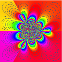
Obviously, as the following examples show, generically for $X\in{\mathscr{E}}(s,r,0)$ the isotropy group $Aut({\widehat{\mathbb{C}}})_{X}$ does not fix $\infty\in{\widehat{\mathbb{C}}}$ (and hence strays from the present work). For further examples and a classification of rational vector fields with finite isotropy on the Riemann sphere, see [3].

Example 4.5.

1. Consider

(11) $$X(z)=\lambda\ \frac{z(z^{n}-1)}{z^{n}+1}\frac{\partial}{\partial z}\in{\mathscr{E}}(n+1,n,0),\text{ for }n\geq 3.$$

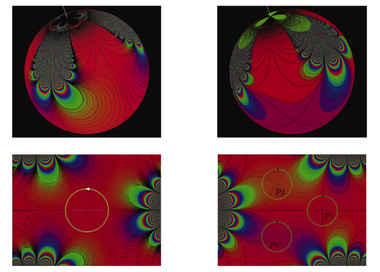
As shown in [3], the isotropy group is a dihedral group $Aut({\widehat{\mathbb{C}}})_{X}\cong\mathbb{D}_{n}$. In this case $\{z\mapsto-{1}/{z}\}\in Aut({\widehat{\mathbb{C}}})_{X}$, hence $\infty\in{\widehat{\mathbb{C}}}$ is not a fixed point of the isotropy group. See Figures 2 (A) and 2 (B).

(A)                              (B)                               (C)                              (D)

Figure 2. Phase portraits of Example 4.5. We have set $\lambda=-i$ so that the zeros of $X$ are centers. (A) and (C) represent the divisors of $X$: zeros appear as red pyramids, poles appear as blue crosses. In (B) and (D) the corresponding phase portraits are visualized. Borders of the strip flows correspond to streamlines of the field. (A) and (B) correspond to (11) with $n=5$ which has isometry group isomorphic to $\mathbb{D}_{5}$. (C) and (D) correspond to (12) which has isometry group isomorphic to $A_{4}$.

From the perspective of Theorem 4.2, ${\widehat{\mathbb{C}}}/\mathbb{D}_{n}={\widehat{\mathbb{C}}}$ and

$$proj:{\widehat{\mathbb{C}}}\longrightarrow{\widehat{\mathbb{C}}},\ \ \ \ \ \ proj_{*}X(w)=n\lambda\frac{w(w-1)}{w+1}\frac{\partial}{\partial w}\doteq Y(w).$$

Moreover, a quick calculation involving partial fractions shows that the distinguished parameter

$\Psi_{X}(z)=\frac{2}{n}\log\left(1-z^{n}\right)-\log(z)$

is multivalued and has $\mathbb{D}_{n}$–symmetry.

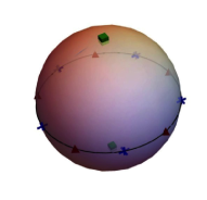
2. Consider

(12) $$X(z)=\lambda\ \frac{4z^{7}+7\sqrt{2}z^{4}-4z}{4z^{6}-20\sqrt{2}z^{3}-4}\frac{\partial}{\partial z}\in{\mathscr{E}}(7,6,0).$$

In this case, as shown in [3], the isotropy group $Aut({\widehat{\mathbb{C}}})_{X}\cong\mathbb{A}_{4}$, the isometry group of the tetrahedron. Note that $\infty\in{\widehat{\mathbb{C}}}$ is a vertex of the corresponding tetrahedron and since the vertices are in the same orbit of $Aut({\widehat{\mathbb{C}}})_{X}$, it follows that $\infty\in{\widehat{\mathbb{C}}}$ is not a fixed point of the isotropy group. See Figures 2 (C) and 2 (D).

Similarly, from the perspective of Theorem 4.2, ${\widehat{\mathbb{C}}}/A_{4}={\widehat{\mathbb{C}}}$ and

$$proj:{\widehat{\mathbb{C}}}\longrightarrow{\widehat{\mathbb{C}}}\ \ \ \ \ proj_{*}X(w)=4\lambda w\frac{\partial}{\partial w}\doteq Y(w).$$

Once again, the distinguished parameter

$\Psi_{X}(z)=-i\left(2\tanh^{-1}\left(\frac{4\sqrt{2}z^{3}}{9}+\frac{7}{9}\right)+\log(z)\right)$

is multivalued and has $A_{4}$–symmetry.

Remark 4.6.

The above behaviour of $\Psi_{X}$ is worth noting: $\Psi_{X}$ is a single valued function if and only if $\omega_{X}$ has zero residue on all its poles.

The cases $s=d=0$ and $r=d=0$ are of special interest.

4.3.1. The families ${\mathscr{E}}(0,r,0)$

A particularly interesting case is ${\mathscr{E}}(0,r,0)$; the condition that $\infty\in{\widehat{\mathbb{C}}}$ is a fixed point of $Aut({\widehat{\mathbb{C}}})_{X}$ is automatically satisfied. In this case, there is a zero of multiplicity $r+2$ at $\infty\in{\widehat{\mathbb{C}}}$, and multi–saddles in ${\mathbb{C}}$.

The family ${\mathscr{E}}(0,r,0)$ appears in W. Kaplan [22] and W. Boothby [10], [11]. On the other hand, M. Morse and J. Jenkins [26] studied whether a foliation on the plane with multi–saddles as singularities can be recognized as the level curves of an harmonic function, see also R. Bott [12], §8, see also [27]. So by using the dictionary, Proposition 4.1, we recognize

$X(z)=\frac{1}{P(z)}\frac{\partial}{\partial z}\ \longleftrightarrow\ \Psi(z)=\int^{z}P(\zeta)d\zeta$.

As an immediate corollary of the Main Theorem we have:

Corollary 4.7 (Analytical and metric classification of ${\mathscr{E}}(0,r,0)$).

1. The families ${\mathscr{E}}(0,r,0)$ and ${\mathscr{E}}(0,r,0)_{id}$ coincide if and only if $r+1$ is prime.

   For $r\geq 2$:

2. $\pi_{1}:{\mathscr{E}}(0,r,0)_{id}\longrightarrow{\mathscr{E}}(0,r,0)_{id}/{Aut({\mathbb{C}})}$ is a holomorphic trivial principal bundle,
   $\pi_{2}\circ\pi_{1}:{\mathscr{E}}(0,r,0)_{id}\longrightarrow{\mathscr{E}}(0,r,0)_{id}/(Aut({\mathbb{C}})\times\mathbb{S}^{1})$ is a real analytic trivial principal bundle.

3. If $X\in{\mathscr{E}}(0,r,0)\backslash{\mathscr{E}}(0,r,0)_{id}$ then there exists a rotation group $\Gamma\cong{\mathbb{Z}}_{\tt k}$ for ${\tt k}\in\mathscr{D}\backslash\{1\}$ and ${\tt k}\not|r$ that leaves invariant

   $$X(z)=\frac{\lambda}{(z-C)^{\nu}\prod\limits_{j=1}^{k_{r}}\prod\limits_{\ell=1}^{\tt k}\Big{[}z-C-(R_{j}{\text{\myfont e}}^{i\alpha_{j}})^{\ell/{\tt k}}\Big{]}}\frac{\partial}{\partial z},$$

   where $r={\tt k}k_{r}+\nu$, $\{R_{j}\}\subset{\mathbb{R}}^{+}$, $\{\alpha_{j}\}\subset{\mathbb{R}}$ and $\nu\in{\mathbb{N}}$.

∎

Furthermore the corresponding normal form is given by (8) with $s=d=0$,

$X(z)=\frac{1}{z^{r}+b_{2}z^{r-2}+\ldots+b_{r}}\frac{\partial}{\partial z}$.

Example 4.8.

1. Consider

$X_{1}(z)=\frac{1}{z(z^{2}-1)}\frac{\partial}{\partial z}\in{\mathscr{E}}(0,3,0)^{S},\quad X_{2}(z)=\frac{1}{z(z^{2}-1)(z^{2}+4)}\frac{\partial}{\partial z}\in{\mathscr{E}}(0,5,0)^{S}.$

Both have isotropy group isomorphic to ${\mathbb{Z}}_{2}$, in agreement with Proposition 3.6, see Figure 3 (A), (B).

2. Let

$X(z)=\frac{\lambda}{z^{3}(z^{4}-1)^{2}(z^{4}-16)}\frac{\partial}{\partial z}\in{\mathscr{E}}(0,15,0).$

Considering the partition $r=15=3+(4+4)+4$, and since $4|(15+1)$, then $Aut({\mathbb{C}})_{X}\cong{\mathbb{Z}}_{4}$ as can readily be seen by checking with (4), see Figure 3 (C).

3. Consider

$X(z)=\frac{\lambda}{z^{2}(z^{3}-1)(z^{3}+8)^{2}}\frac{\partial}{\partial z}\in{\mathscr{E}}(0,11,0).$

From the partition $r=11=2+(3+3)+3$, and since $3|(11+1)$, it follows that $Aut({\mathbb{C}})_{X}\cong{\mathbb{Z}}_{3}$ as can readily be seen by checking with (4), see Figure 3 (D).
Since $r=11=3+4+4$ and $4|(11+1)$, then $Aut({\mathbb{C}})_{X}\cong{\mathbb{Z}}_{4}$ is also possible:

$X(z)=\frac{\lambda}{z^{3}(z^{4}-1)(z^{4}+16)}\frac{\partial}{\partial z}\in{\mathscr{E}}(0,11,0)$

realizes it, see Figure 3 (E).

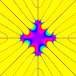
(A)                    (B)                     (C)                     (D)                     (E)

Figure 3. Phase portraits of ${\mathfrak{Re}\left(X\right)}$ in ${\mathscr{E}}(0,r,0)$ having non–trivial isotropy. Borders of the strip flows correspond to streamlines of the field. (A) shows $X\in{\mathscr{E}}(0,3,0)^{S}$, (B) shows $X\in{\mathscr{E}}(0,5,0)^{S}$. Both have isotropy group $Aut({\mathbb{C}})_{X}\cong{\mathbb{Z}}_{2}$, see Example 4.8.1. (C) corresponds to $X\in{\mathscr{E}}(0,15,0)$ with isotropy group isomorphic to ${\mathbb{Z}}_{4}$, see Example 4.8.2. (D) and (E) correspond to $X\in{\mathscr{E}}(0,11,0)$ with (D) having isotropy group isomorphic to ${\mathbb{Z}}_{3}$ and (E) having isotropy group isomorphic to ${\mathbb{Z}}_{4}$, see Example 4.8.3.

4.3.2. The families ${\mathscr{E}}(s,0,0)$

For the case ${\mathscr{E}}(s,0,0)$; the condition that $\infty\in{\widehat{\mathbb{C}}}$ is a fixed point of $Aut({\widehat{\mathbb{C}}})_{X}$ is automatically satisfied for $s\geq 3$: $X$ has a pole of order $2-s$ at $\infty\in{\widehat{\mathbb{C}}}$. Dynamically this corresponds to the case of singularities consisting of centers, sources, sinks and flowers on ${\mathbb{C}}$ and a multi–saddle at $\infty$.

The polynomial vector fields $X\in{\mathscr{E}}(s,0,0)$ have been studied by A. Douady et al. [14], B. Branner et al. [8], M.–E. Frías–Armenta et al. [18], C. Rousseau [31] amongst others.

Once again by the Main Theorem we have.

Corollary 4.9 (Analytical and metric classification of ${\mathscr{E}}(s,0,0)$).

1. The families ${\mathscr{E}}(s,0,0)$ and ${\mathscr{E}}(s,0,0)_{id}$ coincide if and only if $s-1$ is prime.

   For $s\geq 3$:

2. $\pi_{1}:{\mathscr{E}}(s,0,0)_{id}\longrightarrow{\mathscr{E}}(s,0,0)_{id}/{Aut({\mathbb{C}})}$ is a holomorphic trivial principal bundle,
   $\pi_{2}\circ\pi_{1}:{\mathscr{E}}(s,0,0)_{id}\longrightarrow{\mathscr{E}}(0,r,0)_{id}/(Aut({\mathbb{C}})\times\mathbb{S}^{1})$ is a real analytic trivial principal bundle.

3. If $X\in{\mathscr{E}}(s,0,0)\backslash{\mathscr{E}}(s,0,0)_{id}$ then there exists a rotation group $\Gamma\cong{\mathbb{Z}}_{\tt k}$ for ${\tt k}\in\mathscr{D}\backslash\{1\}$ and ${\tt k}\not|s$ that leaves invariant $X$. Furthermore

   $$X(z)=\lambda\ (z-C)^{\nu}\prod\limits_{j=1}^{k_{s}}\prod\limits_{\ell=1}^{\tt k}\Big{[}z-C-(r_{j}{\text{\myfont e}}^{i\theta_{j}})^{\ell/{\tt k}}\Big{]}$$

   where $s={\tt k}k_{s}+\nu$, $\{r_{j}\}\subset{\mathbb{R}}^{+}$, $\{\theta_{j}\}\subset{\mathbb{R}}$ and $\nu\in{\mathbb{N}}$ such that $k|(\nu-1)$. ∎

The corresponding normal form is given by (7) with $r=d=0$, $s\geq 3$, is

$X(z)=(z^{s}+a_{2}z^{s-2}+\ldots+a_{s})\frac{\partial}{\partial z}$.

Example 4.10.

As an example consider ${\mathscr{E}}(7,0,0)$, note that $\mathscr{D}=\{1,3,6\}$. The vector field

$X(z)=z^{4}(z^{3}-1)\frac{\partial}{\partial z}$

has $Aut({\mathbb{C}})_{X}\cong{\mathbb{Z}}_{3}$. In this case, there is a saddle at $\infty\in{\widehat{\mathbb{C}}}_{z}$ with 12 hyperbolic sectors (corresponding to a pole of $X$ of multiplicity $5=7-2$). See Figure 4 for the phase portrait in the vicinity of the origin.

Figure 4. Phase portrait of ${\mathfrak{Re}\left(X\right)}$ for $X(z)=z^{4}(z^{3}-1)\frac{\partial}{\partial z}$ in ${\mathscr{E}}(7,0,0)$, with isotropy group $Aut({\mathbb{C}})_{X}={\mathbb{Z}}_{3}$, see Example 4.10. Borders of the strip flows correspond to streamlines of the field.

The distinguished parameter $\Psi_{X}$ has ${\mathbb{Z}}_{3}$–symmetry and is once again multivalued

$$\Psi_{X}(z)=\frac{1}{3z^{3}}+\frac{1}{3}\log\left(1-z^{3}\right)-\log(z).$$

4.4. Doubly periodic vector fields

Let $w_{1},w_{2}\in{\mathbb{C}}$ determine the period lattice $\Lambda=\{mw_{1}+nw_{2}\ |\ m,n\in{\mathbb{Z}}\}$, and hence the torus $\mathbb{T}={\mathbb{C}}/\Lambda$. We may then consider the Weirstrass $\wp$–function

$$\wp(z)=\wp(z;w_{1},w_{2})=\frac{1}{z^{2}}+\sum_{n^{2}+m^{2}\neq 0}\left(\frac{1}{(z+mw_{1}+nw_{2})^{2}}-\frac{1}{(mw_{1}+nw_{2})^{2}}\right),$$

and its derivative $\wp^{\prime}(z)$. As is well known, letting $x=\wp(z)$, $y=\wp^{\prime}(z)$, $g_{2}$ and $g_{3}$ the Weirstrass invariants, the torus $\mathbb{T}={\mathbb{C}}/\Lambda$ can also be expressed as

(13) $$\mathbb{T}\backslash[0]=\{(x,y)\ |\ y^{2}=4x^{3}-g_{2}\,x-g_{3}\}\subset{\mathbb{C}}^{2},$$

where $[0]$ corresponds to the class of $z=0$ in $\Lambda$, see [2] pp. 272.

Diagram (9) with $M=\mathbb{T}$ and $X(z)=\frac{1}{\wp^{\prime}(z)}\frac{\partial}{\partial z}$ is

with ${\mathcal{R}}_{X}=\Big{\{}\big{(}z,\wp(z)\big{)}\Big{\}}\subset\mathbb{T}\times{\widehat{\mathbb{C}}}_{t}$. Since $\wp(z)$ has a second–order pole at $[0]$, it follows that $X(z)=\wp^{*}(\frac{\partial}{\partial t})$ has zeros of order three at $[0]$ and three simple poles at the classes of the midpoints of the period lattice. Moreover because of (13) the three poles are $\{(x,0)\ |\ 4x^{3}-g_{2}\,x-g_{3}=0\}\subset\mathbb{T}$, see Figure 5 for a particular case.

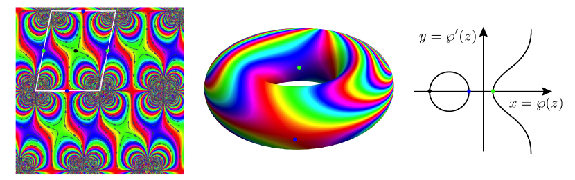
Fundamental domain of $\Lambda$ in ${\mathbb{C}}$                   $\mathbb{T}={\mathbb{C}}/\Lambda$                 $\{y^{2}=4x^{3}-g_{2}\,x-g_{3}\}\subset{\mathbb{C}}^{2}$

Figure 5. Representaton of $X(z)=\frac{1}{\wp^{\prime}(z)}\frac{\partial}{\partial z}$ as in Example 4.4 with $w_{1}=1$, $w_{2}=\frac{1}{4}+\frac{5}{4}i$. On the top figure we have sketched the fundamental domain of ${\mathbb{C}}/\Lambda$ together with the phase portrait of ${\mathfrak{Re}\left(X\right)}$. In the bottom left a representation of the torus $\mathbb{T}$ with the phase portrait of ${\mathfrak{Re}\left(X\right)}$. On the bottom right we have sketched the plane algebraic curve of (13). In all the models for $\mathbb{T}={\mathbb{C}}/\Lambda$ one can observe three simple poles and a zero of multiplicity three.

From the above we can now recognize two examples of symmetries $\Gamma$.

1. Recaling that $\Gamma={\mathbb{Z}}_{2}$ acts on the torus (as a plane algebraic curve), having as generator the hyperelliptic symmetry

$$\mathbb{T}\longrightarrow\mathbb{T},\quad(x,y)\longmapsto(x,-y).$$

It follows that in Diagram (10) $proj_{*}=\wp$ so

$\Big{(}\mathbb{T},X(z)=\frac{1}{\wp^{\prime}(z)}\frac{\partial}{\partial z}\Big{)}\xrightarrow{\ proj_{*}=\wp\ }\Big{(}{\widehat{\mathbb{C}}}=\mathbb{T}/\mathbb{Z}_{2},Y(t)=\frac{\partial}{\partial t}\Big{)}\xrightarrow{\ \Psi_{Y}=Id\ }\big{(}{\widehat{\mathbb{C}}}_{t},\frac{\partial}{\partial t}\big{)}.$

2. As a second example, let $M$ be a (branched) topological cover of $\mathbb{T}$ which inherits the conformal structure from $\mathbb{T}$, then the covering group $\Gamma$ is recognized as a subgroup of the automorphism group of the Riemann surface $M$. Letting $Y(z)=\frac{1}{\wp^{\prime}(z)}\frac{\partial}{\partial z}$ on $\mathbb{T}=M/\Gamma$, clearly $X=proj^{*}Y$. Then in Diagram (10) we can recognize

$(M,X)\xrightarrow{\ proj_{*}\ }\Big{(}\mathbb{T}=M/\Gamma,Y(z)=\frac{1}{\wp^{\prime}(z)}\frac{\partial}{\partial z}\Big{)}\xrightarrow{\ \ \ \Psi_{Y}=\wp\ \ \ }\big{(}{\widehat{\mathbb{C}}}_{t},\frac{\partial}{\partial t}\big{)},$

where ${\mathcal{R}}_{Y}=\Big{\{}\big{(}z,\wp(z)\big{)}\Big{\}}\subset\mathbb{T}\times{\widehat{\mathbb{C}}}_{t}$.

References

- [1] R. D. M. Accola, Strongly branched coverings of closed Riemann surfaces, Proc. Amer. Math. Soc. 26 (1970) 315–322. https://doi.org/10.1090/S0002-9939-1970-0262485-4
- [2] L. V. Ahlfors, Complex Analysis, Third Edition, McGraw–Hill, Inc., (1979).
- [3] A. Alvarez–Parrilla, M. E. Frías–Armenta and C. Yee–Romero, Classification of rational differential forms on the Riemann sphere, via their isotropy group, (2018). https://arxiv.org/abs/1811.04342
- [4] A. Alvarez–Parrilla, J. Muciño–Raymundo, Dynamics of singular complex analytic vector fields with essential singularities I, Conform. Geom. Dyn., 21 (2017), 126–224. http://dx.doi.org/10.1090/ecgd/306
- [5] A. Alvarez–Parrilla, J. Muciño–Raymundo, S. Solorza and C. Yee–Romero, On the geometry, flows and visualization of singular complex analytic vector fields on Riemann surfaces, Proceedings of the workshop in holomorphic dynamics, accepted, (2018). https://arxiv.org/abs/1811.04157
- [6] K. Biswas, R. Perez–Marco, Log-Riemann surfaces, Caratheodory convergence and Euler’s formula Contemporary Mathematics, Volume 639, (2015), 197–203. http://dx.doi.org/10.1090/conm/639/12826
- [7] K. Biswas, R. Perez–Marco, Uniformization of simply connected finite type Log-Riemann surfaces Contemporary Mathematics, Volume 639, (2015), 205–216. http://dx.doi.org/10.1090/conm/639/12827
- [8] B. Branner and K. Dias, Classification of complex polynomial vector fields in one complex variable, J. Difference Equ. Appl. 16 (2010), no. 5–6, 463–517. https://doi.org/10.1080/10236190903251746
- [9] S. A. Broughton, Superelliptic surfaces as –gonal surfaces, in; Riemann and Klein surfaces, automorphisms, symmetries and moduli spaces, Contemp. Math., 629, Amer. Math. Soc., Providence, RI, (2014) 15–28. http://dx.doi.org/10.1090/conm/629/12570
- [10] W. M. Boothby, The topology of regular curve families with multiple saddle points, Amer. J. Math., Vol. 73, No. 2 (Apr., 1951), 405–438. https://www.jstor.org/stable/2372185
- [11] W. M. Boothby, The topology of the level curves of harmonic functions with critical points, Amer. J. Math., Vol. 73, No. 3 (Jul., 1951), 512–538. https://www.jstor.org/stable/2372305
- [12] R. Bott, Marston Morse and his mathematical works, Bull. Amer. Math. Soc. (N.S.) Vol. 3, Num. 3 (1980), 907–950. https://doi.org/10.1090/S0273-0979-1980-14824-7
- [13] I. Dolgachev, Lectures on Invariant Theory, London Mathematical Society Lecture Note Series, 296. Cambridge University Press, Cambridge, (2003). xvi+220 pp. ISBN: 0-521-52548-9.
- [14] A. Douady, J. F. Estrada, P. Sentenac, Champs de vecteurs polynomiaux sur , Unpublished preprint (2005).
- [15] P. Doyle, C. McMullen, Solving the quintic by iteration, Acta Math. 163, 3–4, (1989), 151–180. https://doi.org/10.1007/BF02392735
- [16] J. J. Duistermaat, J. A. C. Kolk, Lie Groups, Springer-Verlag, (1999). https://doi.org/10.1007/978-3-642-56936-4
- [17] H. M. Farkas; I. Kra, Riemann Surfaces, Second edition, Graduate Texts in Mathematics, 71. Springer–Verlag, New York, (1992). https://doi.org/10.1007/978-1-4612-2034-3
- [18] M. E. Frías–Armenta, J. Muciño–Raymundo, Topological and analytic classification of vector fields with only isochronous centers, J. Eqs. Appl., Vol. 19, No. 10, (2013), 1694–1728. https://doi.org/10.1080/10236198.2013.772598
- [19] A. Guillot, Complex differential equations and geometric structures in curves, in: Hernández–Lamoneda L., et al. (eds) Geometrical Themes Inspired by the –body Problem. Lecture Notes in Mathematics, vol 2204. Springer. https://doi.org/10.1007/978-3-319-71428-8_1
- [20] K. Hockett, S. Ramamurti, Dynamics near the essential singularity of a class of entire vector fields, Transactions of the AMS, vol. 345, 2 (1994), 693–703. https://doi.org/10.1090/S0002-9947-1994-1270665-5
- [21] B. Howard, J. Millson, A. Snowden, R. Vakil, The equations for the moduli space of points on the line. Duke Math. J., 146 (2009), no. 2, 175–226.
- [22] W. Kaplan, Topology of level curves of harmonic functions, Trans. A. M. S. 63, 3 (1948), 514–522. https://doi.org/10.1090/S0002-9947-1948-0025159-3
- [23] S. Kerckhoff, H. Masur, J. Smillie, Ergodicity of billiard flows and quadratic differentials, Ann. of Math. 2, 124 (1986), no. 2, 293–311. https://doi.org/10.2307/1971280
- [24] F. Klein, Lectures on the Icosahedron, Dover, New York, (2003). https://books.google.com.mx/books?isbn=0486495280
- [25] J. C. Magaña–Cacéres, Classification of 1–forms on the Riemann sphere up to , Bull. Mexican Math. Soc., (2018). https://doi.org/10.1007/s40590-018-0217-7
- [26] M. Morse, J. Jenkins, The existence of pseudoconjugates on Riemann surfaces, Fund. Math. 39 (1952) (1953), 269–287. https://doi.org/10.4064/fm-39-1-269-287
- [27] J. Muciño–Raymundo, Complex structures adapted to smooth vector fields, Math. Ann., 322, (2002), 229–265. https://doi.org/10.1007/s002080100206
- [28] J. Muciño–Raymundo, C. Valero–Valdéz, Bifurcations of meromorphic vector fields on the Riemann sphere, Ergod. Th. & Dynam. Sys., 15, (1995), 1211–1222. https://doi.org/10.1017/S0143385700009883
- [29] R. Nevanlinna, Analytic Functions, Springer-Verlag, (1970).
- [30] R. Nevanlinna, Über Riemannsche Flächen mit endlich vielen Windungspunkten, Acta Math., 58(1), 295–373, (1932). https://doi.org/10.1007/BF02547780
- [31] C. Rousseau, The bifurcation diagram of cubic polynomial vector fields on , (2015). https://arxiv.org/pdf/1506.07120.pdf
- [32] M. Taniguchi, Explicit representations of structurally finite entire functions, Proc. Japan Acad. Ser. A Math. Sci., Vol. 77, (2001), 68–70. https://projecteuclid.org/euclid.pja/1148393085
- [33] M. Taniguchi, Synthetic deformation space of an entire function, in Value Distribution Theory and Complex Dynamics, Cont. Math., Vol. 303, (2002), 107–136. http://dx.doi.org/10.1090/conm/303/05238
- [34] A. Tyurin, The classical geometry of vector bundles, in Algebraic geometry (Ankara, 1995), 347–378. Lecture Notes in Pure and Appl. Math., 193, Dekker, New York, (1997).