Regular Expression Matching on billion-nodes Graphs

Abstract

In many applications, it is necessary to retrieve pairs of vertices with the path between them satisfying certain constraints, since regular expression is a powerful tool to describe patterns of a sequence. To meet such requirements, in this paper, we define regular expression (RE) query on graphs to use regular expression to represent the constraints between vertices. To process RE queries on large graphs such as social networks, we propose the RE query processing method with the index size sublinear to the graph size. Considering that large graphs may be randomly distributed in multiple machines, the parallel RE processing algorithms are presented without the assumption of graph distribution. To achieve high efficiency for complex RE query processing, we develop cost-based query optimization strategies with only a small size statistical information which is suitable for querying large graphs. Comprehensive experimental results show that this approach works scale well for large graphs.

1 Introduction

Graph data have been widely applied in many area such as knowledge management [20], social network [1], bioinformatics [5], and compilers [21].

In the area, an important application is to retrieve pairs of vertices with specific path between them. For instance, in knowledge management, the information of whether two persons with common characteristics come from the same lineage may be required to extract. It is hard to express by a subgraph or SPARQL query.

As a powerful tool of string pattern description, regular expression can also be used to describe the relationship of vertices in a graph. RE allows querying of arbitrary length paths by using regular expression patterns, it is useful for expressing complex navigation in a graph, in particular, union and transitive closure are crucial when one does not have a complete knowledge of the structure of the knowledge base. In our example, suppose a person $M$ and a person $N$ share a common characteristic. In other words, they share a common attribute values in the knowledge database. If we want to know whether $M$ and $N$ share to the same lineage. This query can be expressed by regular expression easily.

Even some existing work [6, 12, 9, 10, 18, 7, 19] start to study regular expression on graphs, their methods have two shortcomings.

One one hand, existing approaches only consider a share of operations in regular expressions. [6] only studied the regular expression matching on the graph without “or”($|$) and recursion closure. [12, 9, 10] considers only the regular expression matching on tree structure data. Thus, the range of application for these methods is limited.

On the other hand, the scalability is not considered sufficiently. Currently, a graph may scale to very large, even to billion-nodes. For example, FreeBase, the online query processing and services on frequently updating graphs with large size requires lightweight indices. However, [6] requires the structural index with size at least the number of edges of graph. Even though it works efficiently on graphs with small size, it is not suitable for large graphs. [18, 7, 19] do not consider the parallelization of regular expression matching, and they could hardly handle very large graphs that could not reside in a single machine.

To process flexible regular expression on billion-nodes graphs with only a lightweight index, in this paper, a search-based method is proposed. In this method, only an index that retrieves the vertices by their labels is used, which is in size linear to the number of nodes and easy to update. Without structural index, our method is traversal-based.

To avoid large intermediate results, in our system, a lightweight representation of intermediate results is designed. Based on such representation, we propose the basic operators for regular expression processing. For the scalability issues, besides implementation in a single computer, we propose parallel implementation of the operators in a cluster. To find an efficient execution order of the basic operators, a cost-based query optimization strategy for regular expression is proposed with a cost model which requires only small statistics information of graphs. The contributions of this paper are summarized as follows.

• The regular expression query processing on a large graph with full features is studied in this paper. To the best of our knowledge, this is the first paper that studies parallel processing of the full features of regular expression on large graph data.

• With the consideration of the requirement of large graph, we propose a traversal-based strategy for regular expression processing on a large graph. For the convenience of query optimization, we divide query processing into operators. For each operator, efficient implementation algorithms on both single computer and clusters are developed.

• For query optimization of regular expression queries on graph, a cost model is proposed. With the consideration of the feature of large graphs, an estimation strategy requiring only simple statistic information is proposed.

• A dynamic programming algorithm is designed to obtain efficient execution order of operators for regular expression processing based on the estimated cost.

• Extensive experimental results demonstrate that our approaches could accomplish regular expression matching on billion-nodes graphs within 2 seconds and are suitable for various graphs and queries.

Section 2 describes the query language. In Section 3, the framework of regular expression processing is proposed. The logical operator generation is described in Section 3.3. The implementation algorithms of the operators are presented in Section 4. The cost model and query optimization strategy are described in Section 5. Section LABEL:sec:extension discusses extension issues of the proposed approaches. Experiments and analysis are described in Section 6. Section 7 summaries related work and Section 8 concludes the whole paper.

2 Query Language

In many scenarios, the relationship between two vertices in a graph may be complex. In a knowledge base, the relationship between vertices could be naturally represented as the label sequence on the path between them. Thus, to retrieve vertex pairs satisfying requirements in a graph, the query language should describe the label sequence required to be between two vertices. However, with the increase of path length, the relationship between two vertices becomes too complex to be expressed with compact queries with simple semantics.

For instance, $N$ is the offspring of $M$. Obviously, they share the same lineage. In the specific case, we can hardly obtain the length of the path between $M$ and $N$. Thus, it is difficult to express this relationship.

Regular expression is a form of language for sequence in common use. Similar as the regular expression for strings, a regular expression can describe labels attached to the vertices in a path between two vertices in a labeled graph. Hence, a regular expression can be used to describe the requirement of the paths between two vertices in a graph. In the above example, each person has a property ‘status’, it has a label $p$ if he or she has a child and everyone has a label $c$. If $M$ and $N$ come from the same family, the path between $M$ and $N$ must satisfy a criteria: $p-c-p-c-p-c\ldots\ldots$, where we use ‘-’ to denote concatenation to avoid confusion. If we use regular expression to express this criteria, it can be expressed like this: $p(c-p)^{+}c$. Note that reachability queries cannot express such query properly since reachability queries neglect the label in the path.

Formally, the regular expression is defined as following. For the flexibility, the wildcard representing any label is added to the definition.

Suppose the tag set is $\Sigma$. The wildcard is denoted by “#”. The regular expression on $\Sigma$, denoted by $RE(\Sigma)$, is defined as follows.

• $\Sigma\cup\{\#\}\subseteq RE(\Sigma)$

• $\forall r_{1},r_{2}\in RE(\Sigma)$, $r_{1}r_{2}\in RE(\Sigma)$

• $\forall r_{1},r_{2}\in RE(\Sigma)$, $r_{1}|r_{2}\in RE(\Sigma)$

• $\forall r\in RE(\Sigma)$, $r^{+}\in RE(\Sigma)$

• No other expressions are in $RE(\Sigma)$

A data graph is defined as a graph $G$=($V_{G}$, $E_{G}$, $T_{V}$), where $V_{G}$ is the vertex set, $E_{G}$ is the edge set, and $T_{V}:V_{G}\rightarrow\Sigma\cup`\#^{\prime}$ assigns a label to each vertex in $V_{G}$.

If the string $s_{P}$ constructed by connecting the tags in the vertices of a path $P$ from the start node to the end node matches a regular expression $E$, it is said that $P$ matches $E$.

The result of a regular expression $E$ on a data graph $G$ is a set of pairs $R_{E,G}$={($(v_{1},v_{k}$)$|$ a path ($v_{1}$$\rightarrow$$v_{2}$$\rightarrow$$\cdots$$\rightarrow$$v_{k}$) exists in $G$ matches $E$}.

For example, consider the data graph shown in Figure 1. The results of the RE query $Q_{1}$=$a(be|(cd)^{+}f)g$ are {($a_{1}$, $g_{1}$), ($a_{1}$, $g_{2}$), ($a_{1}$, $g_{3}$)}. For $a_{1}$ and $g_{1}$, the path between them $a_{1}b_{1}e_{1}g_{1}$ match the path $abeg$ of the RE. The path $a_{1}c_{2}d_{2}c_{3}d_{3}f_{2}g_{3}$ match the path $a(cd)^{+}fg$ in the RE.

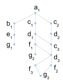
Figure 1: The Data Graph

3 The Framework of RE Query Processing

In this section, we present the framework of RE query processing. Since our goal is to process RE query on large graphs, only lightweight indices with size linear or sublinear to the graph size are permitted. As discussed in [16], with only lightweight index, only simple operators are supported for structural query processing, e.g. traversal and join. RE query processing is to combine such simple operators. Thus, we attempt to process a RE query $r$ by separating $r$ into segments properly, each of which is processed by traversal separately, and joining the results of these segments.

With the consideration of the complexity of RE query, it is difficult to perform the query splitting directly. Thus, we handle the query in two tiers. The first one converts a query to the logical plan, which is near to the form of the query. The second one is to generate the physical plan from the logical plan. Then we discuss these two tiers, respectively.

3.1 Logical Operators

Since a RE includes three basic operations, concentration, alternative operator $|$ and closure operation:⁺, it is natural to match regular expression by turning these basic operations to the matching in a graph. Thus, we define logical operators to support the matching according to the operations in RE.

In RE, the operations concentration and closure are used to describe the connection relationships between nodes in the graph. Concentration means the directly connection between two nodes in a path. Closure means the emergence of node sequences with same label sequence in a path consecutively and repeatedly. The logical operators for RE are defined according to these two operations. To support the operation of ${}^{\prime}|^{\prime}$, each variable in the operator is permitted to match multiple labels in the RE.

The input of the operators may be the nodes matching some labels in the RE or the intermediate results matching a sub expression. With the consideration of input source, corresponding operation in RE and search direction, we summarize 6 logical operators as shown in Table I, where each lowercase letter is a variable referring to a set of labels in RE. In this table, we use ‘-’ to represent ‘$\rightarrow$’ or ‘$\leftarrow$’, which identify the direction of the execution.

TABLE I: The Table of Logical Operators

Operator	Logical Operator	Semantics
concentration	$a-b$	directly concentration between an $a$ node and a $b$ node
	$a-E(b)$	concentration between a $a$ node and the $b$ node in the result of a RE $E$
	$E(b)-a$	concentration between the $b$ node in result of a RE and a $a$ node
	$E_{1}(a)-E_{2}(b)$	concentration of the results of $E_{1}$ and $E_{2}$ on the $a$ and $b$ nodes
Closure	$E(E_{1}(a)-E_{2}(b))^{+}$	the closure of a RE $E$ whose head is an $a$ node as the tail of $E_{1}$, tail is a $b$ node as the head of $E_{2}$, where $E_{1}$ and $E_{2}$ have been processed
	$a^{+}$	the closure of a single label $a$

Intuitively, the processing of an RE query can be converted to a series of logical operators. The logical operators in a regular expression may have multiple possible execution orders. How to generate an efficient execution order is the task of query optimization, wich will be discussed in Section 5.

Example 1 demonstrates the semantics of the logical operators and the framework of regular expression query processing.

Example 1

Consider the query $a(be|(cd)^{+}f)g$ that is processed in from left to right. The first operator is $a\rightarrow(b|c)(\{b,c\})$. The results of this operator are the set of path fragments, each of which matches $a-b$ or $a-c$. Here $b|c$ is a regular expression. $(\{b,c\})$ means that $a$ could be connected to a $b$ or $c$ node.

The following operator is $a(b|c)(\{b\})\rightarrow e$. It means that the $b$ node in a result of $a(b|c)$ connects to an $e$ node. In Figure 1, the results of the subquery $a(b|c)$ are {($a_{1}$, $b_{1}$),($a_{1}$, $c_{1}$),($a_{1}$, $c_{2}$)}. The partial results of $a(b|c)(\{b\})\rightarrow e$ are {($a_{1}$, $e_{1}$),($a_{1}$, $c_{1}$),($a_{1}$, $c_{2}$)}, corresponding to the regular expression $E_{1}=a(be|c)$.

The following operator is closure $(c\rightarrow d)^{+}(E_{1}(c),d)$. The intermediate results in this step are $\{(a_{1}$, $e_{1}$), ($a_{1}$, $d_{1}$), ($a_{1}$, $d_{2}$), ($a_{1}$, $d_{3})\}$ as the results of partial query $E_{2}=a(be|(cd)^{+})$. By processing the operator $E_{2}(d)\rightarrow f$, the intermediate results {($a_{1}$, $e_{1}$), ($a_{1}$, $f_{1}$), ($a_{1}$, $f_{2}$), ($a_{1}$, $f_{3})\}$ are obtained for the partial query $E_{3}=a(be|(cd)^{+}f)$. Then the last operator $E_{3}(\{e,f\})$ $\rightarrow g$ is processed to retrieve the results for the query.

3.2 Physical Operators

To efficiently execute logical operators on large graphs, in this section, we summarize 6 physical operators for them. Each of these operators could be implemented with lightweight index or in absence of index.

Note that when one label exists multiple times in a RE, during query processing, the two existences are treated as two labels and the intermediate results are maintained independently to avoid the confusion. For example,for the RE $cbc^{+}$, the first label $c$ and the last label $c$ in the closure may refer to different node set during query processing. Hence they should be distinguished.

Intuitively, the basic physical operators load nodes from the graph according the label and loading the neighbours with some specific labels. Two operators, Load and Neighbour, are defined for them, respectively.

We also propose two physical operators to link the intermediate results. One links the nodes matching some labels to intermediate results (SingleLink). The other joins of two groups of intermediate results (DoubleLink).

Corresponding to these two logical operators related closure, two special physical operators, ClosureLink and SelfLink, are required as the fixed point of finding the repeated path matching the closure.

According to above discussions, physical operators are summarized in Table II, where each variable may correspond to a set of labels, as is similar as logical operators. For example, for an RE $E$=$(a|bc|def))$, head($E$)={a, b, d}, tail($E$)={a, c, f}. To process the query $(h|r)(a|bc|def)$, supposing that $E$ is processed first, the following logical operator is {h,r}$\rightarrow E(\{a,b,d\})$ corresponding physical operator list is Load({h,r}); Neighbor({h,r}, {a, b, d}); SingleLink({h,r}, {a, b, d}, {a, c, f}).

For SingleLink, it is supposed that the links between $a$ node and $b$ node as well as the links between $b$ nodes and $c$ nodes have been built. For DoubleLink, it is supposed that the links between $a$ nodes and $b$ nodes, $b$ nodes and $c$ nodes , $c$ nodes and $d$ nodes have been built. For ClosureLink, it is supposed the links between $a$ nodes and $b$ nodes have been built.

TABLE II: Physical Operators

Operator	Meaning
Load($a$)	Load the nodes with label $a$
Neighbor($a$, $b$)	Obtain $b$ neighbors of each $a$ nodes and link each $a$ node with its $b$ neighbor
SingleLink($a$, $b$, $c$)	Link the $c$ neighbors of each node with label $b$ to all its $a$ neighbors.
DoubleLink($a$, $b$, $c$, $d$)	Link each pair of $a$ and $b$ nodes where each $a$ node, is a neighbor of a $b$ node $N_{b}$, each $d$ node is a neighbor of a $c$ node $N_{c}$ and $N_{b}$ links $N_{c}$ node
ClosureLink($a$, $b$)	Link each $a$ node $N_{a}$ with all its $b$ descendants with each such $N_{b}$ exits a path $N_{a}N_{b_{1}}N_{a_{1}}\cdots N_{b_{n}}N_{a_{n}}N_{b}$ between them, where $N_{a_{1}}$, $\cdots$, $N_{a_{n}}$ have label $a$; $N_{b_{1}}$, $\cdots$, $N_{b_{n}}$ have label $b$
SelfLink($a$, $a_{1}$, $a_{2}$)	generate a copy of the results of $a$ and link the nodes in two sets referring to the same nodes in the graph.

The relationships between logical operators and physical operators are shown in Table III. In Table III, for closure, the function Link depends on the form of $E_{1}$ and $E_{2}$. If both $E_{1}$ and $E_{2}$ are single labels, this link operator is unnecessary; if only one of $E_{1}$ and $E_{2}$ is a complex regular expression and the other is a single label, the operator is SingleLink; if both of $E_{1}$ and $E_{2}$ are a complex regular expressions, corresponding operator is DoubleLink.

TABLE III: The Relationships between Logical operators and Physical Operators

Logical Operator	Physical Operator List
$a\rightarrow b$	Load($a$); Neighbor($a$, $b$)
$a\leftarrow b$	Load($b$); Neighbor($b$, $a$)
$a\rightarrow E(b)$	Load($a$); Neighbor($a$, $b$); SingleLink($a$, $b$, tail($E$))
$a\leftarrow E(b)$	Neighbor($b$, $a$); SingleLink($a$, $b$, tail($E$))
$E(b)\rightarrow a$	Neighbor($b$, $a$);SingleLink(head($E$), $b$, $a$)
$E(b)\leftarrow a$	Load($a$); Neighbor($a$, $b$));SingleLink(head($E$), $b$, $a$)
$E_{1}(a)\rightarrow E_{2}(b)$	Neighbor($a$),($b$));DoubleLink(head($E_{1}$), $a$, $b$, tail($E_{2}$))
$E(E_{1}(a)-E_{2}(b))^{+}$	ClosureLink($E$);Link(head($E_{1}$), $a$, $b$, tail($E_{2}$))
$a^{+}$	Load($a$), SelfLink($a$, $a_{1}$, $a_{2}$);ClosureLink($a_{1}$,$a_{2}$)

We use an example to illustrate the intermediate results and the physical operator execution.

(a) Results of $L_{1}$

(b) Result of $P_{21}$

(c) Result of $P_{22}$

(d) Result of $P_{31}$

(e) Result of $P_{32}$

(f) Result of $P_{41}$

(g) Result of $P_{42}$

(h) Result of $P_{51}$

(i) Result of $P_{52}$

Figure 2: Intermediate Results

TABLE IV: The Logical Operators and Physical Operators for the Example

LID	Logical operator	PID	Physical Operator
$L_{1}$	$a\rightarrow(b|c)(\{b,c\})$	$P_{11}$	Load($a$)
		$P_{12}$	Neighbor($a$, {$b,c$})
$L_{2}$	$a(b|c)\{b\}\rightarrow e$	$P_{21}$	Neighbor($b$, $e$)
		$P_{22}$	SingleLink($a$, $b$, $e$)
$L_{3}$	$(c\rightarrow d)^{+}(E_{1}(c),d)$	$P_{31}$	ClosureLink($c$, $d$)
		$P_{32}$	SingleLink($a$, $c$, $d$))
$L_{4}$	$E_{2}(d)\rightarrow f$	$P_{41}$	Neighbor($d$,$f$))
		$P_{42}$	SingleLink($a$, $d$, $f$)
$L_{5}$	$E_{3}(\{e,f\})\rightarrow g$	$P_{51}$	Neighbor($\{e,f\}$, $g$)
		$P_{51}$	SingleLink($a$, $\{e,f\}$, $g$)

Example 2

In this example, we show the execution of physical operators for the query and logical operator execution order in Example 1. The corresponding relationships between logical operators and physical operators are shown in Table IV, where the column LID is the id of logical operators and PID is the id of physical operators; the meanings of $E_{1}$, $E_{2}$ and $E_{3}$ are the same as those in Example 1.

The intermediate results for the operators are shown in Figure 2. For the second logical operator $a(b|c)(\{b\})\rightarrow e$, at first, the $e$ neighbor of $b$ nodes are obtained and then SingleLink operator is performed to connect $a$ node with $e$ nodes. For the logical operator $(c\rightarrow d)^{+}(E_{1}(c),d)$, the first physical operator is ClosureLink($c$, $d$), the $c$ nodes as the input include $c_{1}$ and $c_{2}$, but $c_{3}$ is not the input of this operator. The results of the physical operator are ($c_{1}$,$d_{1}$), ($c_{1}$,$d_{2}$), ($c_{1}$,$d_{3}$), ($c_{2}$,$d_{1}$), ($c_{2}$,$d_{2}$) and ($c_{2}$,$d_{3}$). Then $a_{1}$ is connected with $d_{1}$, $d_{2}$ and $d_{3}$.

The efficient implementation algorithms of these physical operators will be discussed in the next section.

3.3 Logical Operator Generation

We explain the conversion from a regular expression to logical operators. Such generation is implemented using postfix expression.

Any infix regular expression can be easily rewritten into a postfix expression. For example, given infix expression $ab-((b-c)|((d|e)-f))-(g|h)$, its postfix expression is $abc-de|f-|-gh|-$. Given a postfix expression, we can generate its logical operators using a tri-column stack in the schema of (operand, prefix, postfix). The operand is the operator, while prefix/postfix column stores the prefix/postfix character set of current stack frame. The algorithm yields a logical operator when meeting concatenation operator “-”, concatenating the postfix of the first operand and the prefix of the second operand. It merges prefixes and postfixes when meeting “or” operator “$|$”, merging the prefixes/postfixes of two operands.

The logical operator generation algorithm consists of three steps:

• Scan the postfix expression from left to right;

• If current character is an operand, then push it to the stack;

• If current character is an operator, pop two operands, doing calculation and push the result back.

4 Implementation Algorithms of Physical Operators

In this section, we will discuss the implementation algorithms of physical operators in Section 3.2. For the convenience of discussions, we introduce centralized algorithms and distributed algorithms in Section 4.1 and Section 4.2, respectively.

4.1 Centralized Algorithms

This section proposes the implementation algorithms for physical operators in centralized environment. Note that the algorithms are implemented with a lightweight index or in absence of index. The description of the algorithms in this section could be easily implemented on a database with join operators.

To simplify the algorithm descriptions, the symbols and functions used in the algorithm descriptions are shown in Table VI.

TABLE V: Symbols in Physical Operator Implementation Algorithms

Symbol	Meaning
$n$	the number of vertices in the graph
$m$	the number of edges in the graph
S($a$)	label set corresponding to the variable $a$ in the operator
link($n_{1}$, $n_{2}$, $r_{1}$, $r_{2}$)	add $n_{1}$ as the $r_{1}$ neighbor of $n_{2}$ and $n_{2}$ as the $r_{2}$ neighbor of $n_{1}$
Filter($l$, $S$)	remove the nodes in $R_{l}$ without any link to the node corresponding to any symbol in $S$
label($k$)	The label of the node $k$

Since the implementation of SelfLink is straightforward, we focus on other operators.

Load The implementation of the physical operator Load is simply load the nodes with label in S($a$) from the graph. With the index that retrieve the nodes according to the label, this operator is performed in time linear to the node number. Such index is called label index, as an inverted list that retrieves the id sets according to the given label, and the size is O($n$).

Neighbor The operator of Neighbor is implemented by load each neighbor with the label in S($b$) for each node in $R_{l}$ ($l\in S(a)$) and link them. At last, the nodes with label in $R_{l}$ without any neighbor with node in S($b$) are filtered. For the efficiency issue, the implementation of this operator requires accessing the neighbors of corresponding nodes and merge their ids with the id set in corresponding entry in the label index or corresponding intermediate node sets to avoid accessing the labels of nodes.

The implementation of the operator Neighbor is shown in Algorithm 1.

Algorithm 1 Neighbor($a$, $b$)

  for each $r_{1}$ in S($a$) do

     for each $n_{1}$ in $R_{r_{1}}$ do

        for each $r_{2}$ in S($b$) do

           load all neighbors of $n_{1}$ with label $r_{1}$ to $N_{n_{1},r_{1}}$

           for each node $n_{2}$ in $N_{n_{1},r_{1}}$ do

              link($n_{1}$, $n_{2}$, $r_{1}$, $r_{2}$)

           $R_{r_{1}}$=$R_{r_{1}}\bigcup N_{n_{1},r_{1}}$

  for each $r_{2}$ in S($b$) do

     filter($r_{2}$, S($a$))

SingleLink and DoubleLink As described in Table II, the goal of SingleLink and DoubleLink is to link nodes in the head and tail in a path. In order to reduce redundancy computation. We apply BFS strategy. As shown in Algorithm 2, at first the nodes in $R_{r_{2}}$ ($r_{2}\in S(b)$) linked by nodes in $R_{r_{1}}$ ($r_{1}\in S(a)$) are collected in $M$. (Line 3-Line 5) Then for each node $n^{\prime}$ in $M$, the nodes with nodes in $R_{r_{3}}$ ($r_{3}\in S(c)$) linked by $n^{\prime}$ (Line 6-Line 9). At last, the nodes in each $R_{r_{1}}$ and each $R_{r_{3}}$ are filtered based on their links (Line 10 and Line 12). As shown in Algorithm 3, the implementation of DoubleLink is similar as SingleLink but with an additional step of collection neighbors in $R_{r_{3}}$ ($r_{3}\in S(c)$) for each node in $M$ (Line 7-Line 9).

Algorithm 2 SingleLink($a$, $b$, $c$)

1:  for each $r_{1}$ in S($a$) do

2:     for each $n_{1}$ in $R_{r_{1}}$ do

3:        $M$=$\varnothing$

4:        for each $r_{2}$ in S($b$) do

5:           $M$=$M\cup N_{n_{1},r_{1}}$

6:        for each $n^{\prime}$ in $M$ do

7:           for each $r_{3}$ in S($c$) do

8:              for each $n_{2}$ in $N_{n^{\prime},r_{3}}$ do

9:                 link($n_{1}$, $n_{2}$, $r_{1}$, $r_{3}$)

10:     Filter($r_{1}$, S($c$))

11:  for each $r$ in S($c$) do

12:     Filter($r$, S($a$))

For example, to perform the operator SingleLink($a$, {$e$,$f$}, $g$) on the result in Figure 2(h), at first, $e$ and $f$ nodes connected to $a$ node are obtained. The set of $e$ and $f$ nodes connected to $a_{1}$ is $S_{1}$={$e_{1}$, $f_{1}$, $f_{2}$, $f_{3}$}. As the result, the $g$ nodes as the neighbors in the nodes in $S_{1}$ are obtained. Then, the set {$g_{1}$,$g_{2}$,$g_{3}$} is obtained and $a_{1}$ is linked with $g_{1}$,$g_{2}$ and $g_{3}$.

Algorithm 3 DoubleLink($a$, $b$, $c$, $d$)

1:  for each $r_{1}$ in S($a$) do

2:     for each $n_{1}$ in $R_{r_{1}}$ do

3:        $M$=$\O$

4:        for each $r_{2}$ in S($b$) do

5:           $M$=$M\cup N_{n_{1},r_{2}}$

6:        $H$=$\O$

7:        for each $n^{\prime}$ in $M$ do

8:           for each $r_{3}$ in S($c$) do

9:              $H$=$H\cup N_{n^{\prime},r_{3}}$

10:        for each $n^{\prime\prime}$ in $H$ do

11:           for each $r_{3}$ in S($d$) do

12:              for each $n_{2}$ in $N_{n^{\prime},r_{3}}$ do

13:                 link($n_{1}$, $n_{2}$, $r_{1}$, $r_{3}$)

14:     Filter($r_{1}$, S($d$))

15:  for each $r$ in S($d$) do

16:     Filter($r$, S($a$))

ClosureLink The pseudo code of the implementation algorithm of ClosureLink is shown in Algorithm 4. The idea is to obtain the nodes to connect with $ClosureSearch$. During the search, to avoid repeated search, we use a hash table $H$ to maintain $a$ with all descendants searched. For each vertex $n$ matching $a$, a descendant set $M_{n}$ is generated for all corresponding $b$ vertices by $ClosureSearch$.

To avoid redundant search, $ClosureSearch$ is implemented in the combination of DFS and BFS. For each vertex $n$ with label $a$, BFS is applied to collect all its $b$ neighbors in $H_{b}$ and add all the neighbors to the $a$ ancestors of $n$ in $S$ (Line 16-Line 19). Then, for each node $n^{\prime}$ in $H_{b}$, DFS is applied to obtain all its $a$ ancestors and $b$ ancestors. $ClosureSearch$ is invoked for each unvisited $a$ neighbor $n^{\prime\prime}$ of $n^{\prime}$ (Line 25). If $n^{\prime\prime}$ has been visited, the corresponding $b$ nodes are copied to the ancestors (Line 27-Line 32).

For example, to perform the ClosureLink($c$,$d$) on the $c$ node set {$c_{1}$,$c_{2}$}, $c_{1}$ is to be processed at first and pushed to the stack $S$. $d_{1}$ is added to $H_{b}$ and $M_{c_{1}}$. Then, the traversal starts from $d_{1}$, and $c_{3}$ is obtained. $c_{3}$ is pushed to $S$. The traversal starting from $c_{3}$ obtains $d_{2}$ and $d_{3}$. $d_{2}$ and $d_{3}$ are added to $M_{c_{1}}$ and $M_{c_{3}}$. When the search from $c_{1}$ is accomplished, $c_{1}$ is linked to all vertices in $M_{c_{1}}$. After that, since $c_{3}$ has been visited, $c_{3}$ is linked to all vertices in $M_{c_{3}}$.

Note that descendants may have duplications. It is caused by repeated segments in the graph matching the clause in the RE. Such duplications could be avoided by adding links to sets instead of copying sets (in Line 29 and Line 32). From the experiments, such cases seldom occur.

Algorithm 4 ClosureLink($a$, $b$)

1:  $H$=$\O$

2:  for each $l$ in L($a$) do

3:     for each $n$ in $R_{l}$ do

4:        if $n$ is not in $H$ then

5:           $M_{n}$ = $\O$

6:           $S$ = $\O$

7:           ClosureSearch($n$, $l$, $a$, $b$, $M_{n}$, $H$, $S$)

8:        add $n$ to $H$

9:        for each $k$ in $M_{n}$ do

10:           link($n$, $k$, $r$, label($k$))

11:  ClosureSearch($n$, $l$, $a$, $b$, $M$, $H_{a}$, $S$)

12:  Push($S$, $n$)

13:  $H_{b}$=$\varnothing$

14:  for each $l$ in S($b$) do

15:     for each $j$ in $N_{n,l}$ do

16:        for each $k$ in $S$ do

17:           if $j\in R_{l}$ then

18:              add $j$ to $M_{k}$

19:              add $j$ to $H_{b}$

20:     for each $n^{\prime}$ in $H_{b}$ do

21:        for each $l^{\prime}$ in S($a$) do

22:           $TH$=LoadNeighbor($n^{\prime}$, $l^{\prime}$)

23:           for each $n^{\prime\prime}$ in $TH$ do

24:              if $n^{\prime\prime}\notin H_{a}$ and $n^{\prime\prime}\notin S$ then

25:                 ClosureSearch($n^{\prime\prime}$, $l^{\prime}$, $a$, $b$, $M_{n^{\prime\prime}}$, $H_{a}$, $S$)

26:                 add $n^{\prime\prime}$ to $H_{a}$

27:              else if $n^{\prime\prime}\in H_{a}$ then

28:                 for each $r$ in $S$ do

29:                    $M_{r}$=$M_{r}\cup M_{n^{\prime\prime}}$

30:              else

31:                 for $r$=top($S$) to prior($n^{\prime\prime}$) do

32:                    $M_{r}$=$M_{r}\cup M_{n^{\prime\prime}}$

33:  POP($S$)

Note that during the operator processing, the original graph is not modified. When a vertex $n$ in the graph is obtained, a stub node for $n$ is constructed in the intermediate result. During traversal, the adding of a link between $n$ and other node $m$ is implemented by adding such link between corresponding stub nodes.

Complexity Analysis For a graph with $n$ vertices and $m$ edges, obviously, in the worst case, the time complexity of operator Load and SelfLink is O($n$) since at most each vertex is accessed only once. In the worst case, for each vertex $v$, the operator Neighbor will access at most $n$ vertices. Then the time complexity of $Neighbor$ is O($n^{2}$).

With BFS search strategy, for each step, each dummy vertex is processed only once and for each vertex the vertices with special labels linked to it will be visited. Therefore, the time complexities of SingleLink and DoubleLink are both O($n^{2}$).

With the hash table in the ClosureLink, each vertex in the graph is visited at most once and for each visited vertex, only the vertices with special labels linked to it are to be accessed, the number of which is at most $n$. Therefore, the time complexity of ClosureLink in the worst case is O($n$). Since each logical operator corresponds a constant number of physical operators and for each RE, the number of logical operators equals to the number of concentration and closure operators $k$, the time complexity in the worst case of RE query processing is O($kn^{2}$).

4.2 Distributed Algorithms

To handle very large graphs, it naturally adopts a distributed platform. In order to process regular expression query on large distributed graphs efficiently, our solution provides efficient physical operator implementation algorithms on the distributed platform to minimize the communication cost. From the aspect of graph management, the possible communication cost is caused by traversing from the vertex in one machine to those in another machine. Thus, we should select the distributed graph management platform supporting efficient traversal.

Motivated by this, we adopt infrastructure of Microsoft Graph Engine , an open-source distributed in-memory graph processing engine which supports traversal efficiently. It is underpinned by a strongly-typed in-memory key-value store and a general-purpose distributed computation engine. The following two core capabilities of Graph Engine make it an ideal platform for handling distributed large graphs with complex data schema: 1) It excels at managing a massive amount of distributed in-memory objects and providing efficient random data access over the distributed data. Fast random access is the key to many graph algorithms. 2) It excels at handling big graph data with complex schema. For example, Graph Engine is serving a Microsoft knowledge graph (about 23 TB) which has thousands of entities types and billions of nodes and edges.

Thus, such platform is suitable for efficient distributed implementation of Neighbor, SingleLink, DoubleLink and ClosureLink.

In distributed environment, for the convenience of processing, each node is stored locally, and only the ids of nodes are transmitted during query processing.

With the consideration of network issues, the Load and SelfLink are only performed locally. However, for other operators, the network communications may be involved.

Clearly, a pretty graph partition among the machines in a cluster could accelerate the processing. However, the graph partition is costly in computation especially for very large graphs. Additionally, in real-world scenarios, the workload on a graph distributed in a cluster may contain various operations instead of only regular expression query processing. Thus, it is difficult to choose a proper partition criteria. To make our approach suitable for real applications, we suppose that the graph is partitioned among machines randomly without any sophisticated graph partition strategy.

Basic Operations From the implementation strategy, the basic operations related to two nodes are fetching a neighbor from a node and connecting two nodes. Therefore, the queries are processed in distributed environment by two network primitives according to the two operations for the nodes distributed in different machines in the network.

• GetNeighbor($n$, $t_{r}$, $t_{n}$) obtains the neighbors with tag $t_{r}$ for the nodes $n$ with tag $t_{n}$.

• AddLink($u$, $v$, $a$, $b$) connects $u$ and $v$ with $u$ as $v$’s a neighbor and $v$ as $u$’s b neighbor.

In order to save the communication cost and network bandwidth, the distributed implementation has two strategies. One is to load node ids instead of all information of nodes. The other is to load and revise link in batch style. The batch-style operators are BatchGetNeighbor and BatchAddLink, respectively. The input of BatchGetNeighbor is a table in schema ($id$, $r_{1}$, $r_{2}$), with the same semantics as that of GetNeighbor. The returned results are in schema ($pid$,$plabel$,$cid$,$clabel$), where $pid$ is the id of the input tuple, $plabel$ is its label, $cid$ is the id of the obtained neighbor, and $clabel$ is the label of the neighbor. The input of BatchAddLink is in schema ($pid$,$plabel$,$cid$,$clabel$), where $pid$ is the id of the input tuple, $plabel$ is its label, $cid$ is the id of the neighbor, and $clabel$ is the label of this neighbor to link.

In the intermediate results, for each node, the links to neighbors are the ids of the node. In each machine, to access the real node efficiently, a hash table is maintained to map the id to the real node. And in the whole system, the id of computer for each node $n$ is encoded in the id of $n$.

SingleLink, GetNeighbour and DoubleLink, The implementation of SingleLink operator share the same flow as Algorithm 2. The difference is that the functions of BatchGetNeighbor and BatchAddLink are invoked for execution in batch. The pseudo code of the implementations of SingleLink operators is shown in Algorithm 5. Such algorithm is executed in all machines in the system. The batch execution steps are in Line 11 and Line 15, respectively. During the invocation of these two functions, these tasks related to the same computer are sent to it in batch.

Algorithm 5 DistributedSingleLink($a$, $b$, $c$)

  for each $r_{1}$ in S($a$) do

     for each $n_{1}$ in $R_{r_{1}}$) do

        $M$=$\varnothing$

        for each $r_{2}$ in S($b$) do

           for each $n_{2}$ in $N_{n_{1},r_{2}}$ do

              add ($n_{1}$, $r_{1}$, $n_{2}$, $r_{2}$) to $T_{1}$

  for each $t$ in $R_{1}$ do

     add ($t[pid]$, $t[plabel]$) to $M_{t[cid],t[clabel]}$

     for each $r$ in S($c$) do

        add($t[cid]$, $t[clabel]$, $r$ to $T_{2}$)

  $R_{2}$=BachGetNeighbor($T_{2}$)

  for each $t$ in $R_{2}$ do

     for each $r$ in $M_{t[pid],t[plabel]}$ do

        add ($r[id]$, $r[label]$, $t[cid]$, $t[clabel]$) to $T_{3}$

  BatchAddLink($T_{3}$)

  for each $r_{1}$ in S($a$) do

     Filter($r_{1}$, S($c$))

  for each $r_{2}$ in S($c$) do

     Filter($r_{2}$, S($a$))

We use an example to illustrate the distributed implementation of SingleLink. The distributed implementation of DoubleLink and Neighbor are similar.

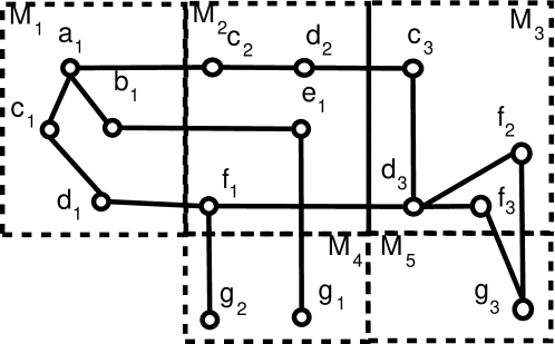
Figure 3: The distributed Graph

Example 3

Consider the process of $Q_{1}$ in the graph in Figure 1. It is supposed that there five computers $M_{1}$ $\cdots$ $M_{5}$ in the cluster. The partition of nodes in the cluster is shown in Figure 3. For the execution physical operator SingleLink($a$, {$e$,$f$}, $g$) on the intermediate results shown in Figure 2, at first, starting from $a_{1}$, the network primitives of GetNeighbor($a_{1}$, {$e_{1}$,$f_{1}$}, $g$) and GetNeighbor($a_{1}$, {$f_{2}$,$f_{3}$}, $g$) are generated. Then, they are sent to $M_{2}$ and $M_{3}$, respectively. After $M_{2}$ and $M_{3}$ executed the primitives. The ids of $g_{1}$, $g_{2}$ and $g_{3}$ are returned to $M_{1}$. $a_{1}$ is linked with $g_{1}$, $g_{2}$ and $g_{3}$. With these ids, the locations of $g_{1}$, $g_{2}$ and $g_{3}$ are known. With these locations, the primitives of link, AddLink($a_{1}$, {$g_{1}$, $g_{2}$}, $a$, $g$) and AddLink($a_{1}$, $g_{3}$, $a$, $g$), are generated and sent to $M_{4}$ and $M_{5}$, respectively. With these primitives, in $M_{4}$, $g_{1}$ and $g_{2}$ are linked with $a_{1}$, and in $M_{5}$, $g_{3}$ is linked with $a_{1}$.

ClosureLink DFS in Algorithm 4 may access a remote machine multiple times for each round of iteration. However, since multiple remote accessing involve large communication cost, the implementation of ClosureLink on a distributed graph tries to avoid DFS. Instead, as shown in Line 17 and Line 27 in Algorithm 6, $a$ and $b$ nodes are obtained in batch. Then, Line 31 adds corresponding links in the intermediate results in batch.

Algorithm 6 DistributedClosureLink($a$, $b$)

1:  $H$=$\varnothing$

2:  for each $l$ in S($a$) do

3:     for each $n$ in $R_{l}$ do

4:        for each $l^{\prime}$ in S($b$) do

5:           if ($n$, $l$, $l^{\prime}$) is not in $H$ then

6:              add ($n$, $l$, $l^{\prime}$) to $H$

7:              for each $n^{\prime}$ in $N_{n,l^{\prime}}$ do

8:                 add ($n$, $l$, $n^{\prime}$, $l^{\prime}$) to $R_{1}$

9:  while $R_{1}\neq\varnothing$ do

10:     $N$=$\varnothing$

11:     for each $t$ in $R_{1}$ do

12:        add ($t[plabel]$, $t[pid]$) to $M_{1}[(t[clabel],t[cid])]$

13:        ($t[clabel]$, $t[cid]$) to $N$

14:     for each $t$ in $N$ do

15:        for each $l$ in S($a$) do

16:           add ($t[cid]$, $t[clabel]$, Label($l$)) to $T_{2}$

17:     $R_{2}$ = BatchGetNeighbor($T_{2}$)

18:     $N$=$\varnothing$

19:     for each $t$ in $R_{2}$ do

20:        add $M_{1}(t[plabel],t[pid]$) to $M_{2}[(t[clabel],t[cid])]$

21:        ($t[clabel]$, $t[cid]$) to $N$

22:     for each $t$ in $N$ do

23:        for each $l^{\prime}$ in L($b$) do

24:           if ($n$, $l$, $l^{\prime}$) is not in $H$ then

25:              add ($n$, $l$, $l^{\prime}$) to $H$

26:              add ($n$, $l$, $l^{\prime}$) to $T_{1}$

27:     $R_{1}$=BatchGetNeighbor($T_{1}$)

28:     for each $t$ in $R_{1}$ do

29:        for each $r$ in $M_{2}[(t[plabel],t[pid])]$ do

30:           add ($r[id]$, $r[label]$, $t[cid]$, $t[clabel]$) to $T_{3}$

31:     BatchAddLink($T_{3}$)

32:  for each $r_{1}$ in S($a$) do

33:     Filter($r_{1}$, S($b$))

34:  for each $r_{2}$ in S($b$) do

35:     Filter($r_{2}$, S($a$))

Example 4 is used to show that processing of the distributed implementation of ClosureLink.

Example 4

To process ClosureLink($c$, $d$) on the graph in Figure 1 with graph partition in Figure 3. At first, the search starts from $c_{1}$ and $c_{2}$ in $M_{1}$ and $M_{2}$, respectively. As the result, $d_{1}$ and $d_{2}$ are obtained. The primitives GetNeighbor($d_{1}$, $c$, $d$) and GetNeighbor($d_{2}$, $c$, $d$) then request $c$ nodes from $M_{3}$. They are processed in $M_{3}$ in batch. From the information stored in $c_{3}$, the ids of $d_{1}$, $d_{2}$ and $d_{3}$ are sent to $M_{1}$ and $M_{2}$, respectively.

In $M_{1}$, $c_{1}$ is linked with $d_{2}$ and $d_{3}$, and the primitives AddLink($c_{1}$,$d_{2}$, $c$, $d$) and AddLink($c_{1}$, $d_{3}$, $c$, $d$) are generated and sent to $M_{2}$ and $M_{3}$, respectively. In $M_{2}$, $c_{2}$ is linked with $d_{1}$ and $d_{2}$, and the primitive AddLink($c_{2}$,$d_{1}$, $c$, $d$) and AddLink($c_{2}$, $d_{3}$, $c$, $d$) is generated. They are sent to $M_{1}$ and $M_{2}$, respectively.

Then, in $M_{1}$, $d_{1}$ is connected with $c_{3}$; in $M_{2}$, $d_{2}$ is linked with $c_{1}$; in $M_{3}$, $c_{1}$ and $c_{2}$ are linked with $d_{3}$. From the aspect of $M_{1}$, the search then starts from $d_{2}$ with $c_{1}d_{1}c_{3}d_{2}$ as the traversal path. $c_{2}$ is obtained. Since $c_{2}$ has no other $d$ neighbor. The traversal in $M_{1}$ halts. Similar process is performed in $M_{2}$.

5 Query Optimization

As discussed in Section 3, each RE query may have different processing orders and directions of the operators. The execution order may affect the efficiency of query processing. For example, even for the simple query $abc$, it is supposed that each of 1G nodes with tag $a$ is linked with one different $b$ node and only one of the $b$ nodes is connected with a $c$ node. If the query is executed in the direction from $a$ to $c$, more than 2G nodes are accessed during search, while only two nodes are accessed if the query is executed from $c$ to $a$.

Motivated by this, in this section, we develop the query optimization strategy for RE queries. As the base of query optimization, we propose the cost estimation methods for operators and the size of intermediate results in Section 5.1.

5.1 Estimation

In this section, we propose a cost-based query estimation method for query optimization. Since for a large graph, it is impossible to maintain a global sketch with size super linear to the graph size. Therefore, in our system, only following statistic information is kept, which is independent to the graph size.

1. The number of the nodes with label $l$, denoted by $Num(l)$

2. The average neighbor number of the nodes with label $l$, denoted by $Neighbor(l)$.

3. The probability of a node with label $l_{1}$ has at least one neighbor with label $l_{2}$ respectively, denoted by $Pro(l_{1},l_{2})$.

4. The average number of the neighbor with label $l_{2}$ of a node with label $l_{1}$ if it has at least one neighbor with $l_{2}$, denoted by $T_{Neighbor}(l_{1},l_{2})$

Such information is computed by traversing the graph once. In a large graph, the size of $Num(l)$ and $Neighbor(l)$ for all labels is linear to the size of the label number $L$. However, the size of of $Pro$ and $T_{N}eighbor$ is $L^{2}$. In order to deal with the graph with a large number of labels, we use two thresholds $\epsilon_{P}$ and $\epsilon_{T}$. For two labels $l_{1}$ and $l_{2}$, if $Pro(l_{1},l_{2})<\epsilon_{T}$, a small value $\delta_{p}$ is used instead of the real value of $Pro(l_{1},l_{2})$. Similarly, if $T_{N}eighbor(l_{1},l_{2})<\epsilon_{T}$, the real value of $T_{Neighbor(l_{1},l_{2})}$ is replaced by a small value $\delta_{T}$ during optimization. Thus, the small size of statistic information is ensured.

Based on above statistics information, we introduce the estimation approach. As discussed in Section 4, one label may exist multiple times in a RE corresponding to different set of intermediate results. During query processing, the size of intermediate results will change. In order to distinguish multiple occurrences of the same label in the optimization, we assign a uniform id for the occurrences of each label and use L($x$) to denote the corresponding label of the label with id $x$. We use $I_{x}$ to denote the set of intermediate results corresponding to $x$. In the remaining part of this section, without explicitly explanation, the variables in the operators and formulas refer to a set of ids instead of labels.

For the convenience of discussions, we discuss the estimation of operators without ’$|$’ as the basic version. Then we discuss the extension to the operators with ’$|$’

5.1.1 The Estimation of Operators without ’$|$’

For the brief of discussion, in the beginning, we focus on the estimation for operators without ‘$|$’. The subqueries with ‘$|$’ will be discussed later. It means that each variable refers to single id.

TABLE VI: Symbols in Estimation

Symbol	Meaning
$Link^{\prime}(a,b)$	the average number nodes in $I_{b}$ linked by each node in $I_{a}$ after the operator computation
$Link(a,b)$	the average number nodes in $I_{b}$ linked by each node in $I_{a}$ before the operator computation
$size^{\prime}(a)$	the size of $I_{a}$ before the operator computation
$size(a)$	the size of $I_{a}$ after the operator computation

Basic Information The cost estimation is based on the sizes of intermediate results and the number of links between the nodes in two intermediate result sets. Thus, we discuss the estimation of such parameters at first. The symbols used in such estimation are described in Table VI. Then we discuss the size and link number estimation in the following paragraphs. The results are summarized in Table VII, where the column Link is the number of links between of two sets of intermediate results, and column Size is the numbers of the intermediate results.

Result Size of SingleLink and DoubleLink The estimated size of Load and SelfLink is intuitively the number of corresponding nodes. We use SingleLink as an example to explain the idea of the estimation SingleLink and DoubleLink. For the operator SingleLink, Link($a$,$b$)Pro($b$,$c$) is the average number of links between $I_{a}$ and the nodes in $I_{b}$ with at least one $c$ node. With Link($b$,$c$) as the average number of links between $I_{b}$ and $I_{c}$, for each node in $I_{b}$, the estimated link number between $I_{a}$ and $I_{b}$ is multiplied by Link($b$,$c$) to compute the average number of links between each node in $I_{a}$ and the nodes in $I_{c}$ through some nodes in $I_{b}$. Since each node $n$ in $I_{a}$ is connected with a node in $I_{b}$, the probability of $n$ links with at least a node in $I_{c}$ through the node in $I_{b}$ is the probability that a node in $I_{b}$ links to at least a node in $I_{c}$. The estimation of the size of $I_{c}$ after the operator execution is similar.

Result Size of ClosureLink In the formula of estimated links in ClosureLink($a$, $b$), $t$ means the average number of link between each $b$ node $n_{b}$ in $I_{b}$ and the node in $I_{b}$ through the path $n_{b}-n_{a}-n_{b}^{\prime}$, where $n_{a}\in I_{a}$ and $n_{b}^{\prime}\in I_{b}$. In $t$, Pro($b$, $a$)$T_{Neighbor}(b,a)$ is the average number of the neighbors with label L($a$) of each node of $I_{b}$ and Pro($b$, $a$)$T_{Neighbor}(b,a)$ is the average number of nodes with label L($a$) of each node of $I_{b}$. Pro($a$, $b$)$link^{\prime}(a,b)$ is the average number of nodes with label L($b$) linked by each node with label L($a$) in the intermediate result. Hence, $t$ represents the average number of nodes in $I_{b}$ of each node in $I_{a}$ with a path $a-b$ between them. Since the computation of ClosureLink requires the traversal of the paths in label form $a-b-a-\cdots-a-b$ with the all possible lengths, the average number of links in the results is estimated as link’($a$, $b$)+ link’($a$, $b$)$t$+ $\cdots$ +link’($a$, $b$)$t^{k}$ + $\cdots$. When $t\leq 1$, since the maximal number of links between each node in $I_{a}$ and the nodes in $I_{b}$ is $size^{\prime}(b)$, the estimation of average node number in $b$ lined with each node in $I_{a}$ is $size^{\prime}(b)$. Since before ClosureLink operation, each node in $I_{a}$ has been linked with at least one node in $I_{b}$, and each node in $I_{b}$ has been linked with at least one node in $I_{a}$, the size of $I_{a}$ and $I_{b}$ are not changed after the operation.

TABLE VII: The Intermediate Result Size of Operators

Operator	Link	Size
Load($a$)	-	size($a$)=Num($a$)
Neighbor($a$, $b$)	$size^{\prime}(a)$Pro($a$,$b$)Neighbor(L($b$))	size($a$)=$size^{\prime}(a)$Pro($a$,$b$); size($b$)=Num($b$)Pro($b$,$a$)
SingleLink($a$, $b$, $c$)	Link($a$,$b$)Pro($b$,$c$)Link($b$,$c$)	size($a$)=$size^{\prime}(a)$Pro($b$,$c$); size($c$)=$size^{\prime}(c)$)Pro($b$,$a$)
DoubleLink($a$, $b$, $c$, $d$)	Link($a$,$b$)Pro($b$,$c$))Link($b$,$c$)Pro($c$,$d$)Link($c$,$d$)	size($a$)=$size^{\prime}(a)$Pro($b$,$c$)Pro($c$,$d$); size($d$)=$size^{\prime}(d)$Pro($c$,$b$)Pro($b$,$a$)
ClosureLink($a$, $b$)	Link($a$,$b$)$\frac{1}{1-t}$($t<1$); $size^{\prime}(b)$ ($t>1$); $t$=Pro($b$, $a$)$(T_{Neighbor}(b,a)-1)$Pro($a$, $b$)$(Link^{\prime}(a,b)-1)$	size($a$)=$size^{\prime}(a)$; size($b$)=$size^{\prime}(b)$
SelfLink($a$)	Num($a$)	size($a$)=Num($a$)

With this information, the cost estimation formulas of physical operators are shown in Table VIII.

Cost of SingleLink and DoubleLink Since the operators Load and SelfLink access each node in the candidate only once, their costs are the same as the number of candidates. The operator SingleLink has two phases, the first phase collects the nodes in $I_{b}$ for the nodes in $I_{a}$ with cost as $size^{\prime}(a)$Link($a$,$b$), and the second phase collects the nodes in $I_{c}$ linked with nodes in $I_{a}$ with cost $size^{\prime}(a)$Link($a$,$b$)Link($b$, $c$). The estimation for DoubleLink is similar.

Cost of ClosureLink As shown in Algorithm 4, the operator ClosureLink has multiple phases, each phase has two steps. The first is to obtain the nodes in $I_{b}$ that is connected with the nodes in $I_{a}$ which require to access the neighbors of each node in $I_{b}$. From the aspect of starting from a single node in $I_{a}$, in the first step, the cost is Link’($a$,$b$). In the first step of the next phase, the number of the starting nodes in $I_{a}$ is size’($b$)pro($b$,$a$)$\frac{size^{\prime}(a)}{Num(a)}$, since the number of all nodes with label L($b$) in the second step of the last phase is size’($b$). The cost of the first step in the second phase is size’($b$)pro($b$,$a$)$\frac{size^{\prime}(a)}{Num(a)}$Link’($a$,$b$). With the assumption that the share of intermediate results in $I_{b}$ is linear with the that in $I_{a}$, the number for nodes in $I_{b}$ in this step is

$$\scriptsize size^{\prime}(b)pro(b,a)\frac{size^{\prime}(a)}{Num(a)}\frac{size^{\prime}(b)}{size^{\prime}(a)}=size^{\prime}(b)pro(b,a)\frac{size^{\prime}(b)}{Num(a)}$$

Therefore, the number of nodes in $I_{a}$ as the input of the first step of the third phase is

$$size^{\prime}(b)Pro(b,a)\frac{size^{\prime}(b)}{Num(a)}Pro(b,a)\frac{size^{\prime}(a)}{Num(a)}$$

Therefore the cost of the first step of the $k$th phase ($k>1$) is size’($b$)$r^{k-1}\frac{size^{\prime}(b)}{size^{\prime}(a)}$Link’($a$,$b$), where $r$=Pro($b$,$a$)$\frac{size^{\prime}(a)}{Num(a)}$. With the consideration that all $b$ nodes are accessed only once, the cost of the second step of all the phases is I($b$)$T_{Neighbor}(b,a)$. For the case that $r$ is larger than 1, the cost is estimated as the maximum cost of search all possible nodes with labels L($a$) and L($b$).

TABLE VIII: The Cost of Operators

Operator	Cost
Load($a$)	Num(L($a$))
Neighbor($a$, $b$)	$size^{\prime}(a)$Neighbor(L($a$))
SingleLink($a$, $b$, $c$)	$size^{\prime}(a)$Link($a$,$b$)(1+Link($b$,$c$))
DoubleLink($a$, $b$, $c$, $d$)	$size^{\prime}(a)$Link($a$,$b$)(1+Link($b$,$c$)(1+Link($c$,$d$)))
ClosureLink($a$, $b$)	size’(a)Link’($a$,$b$)+$\frac{(size^{\prime}(b))^{2}}{size^{\prime}(a)}$$\frac{1}{1-r}$Link’($a$,$b$) + $I$($b$)$T_{Neighbor}(b,a)$ ($r<1$)
	Num($a$)$T_{Neighbor}(a)$+Num($b$)$T_{Neighbor}(b)$ ($r>1$)
SelfLink($a$)	size($a$)

5.1.2 The Estimation of Operators with ‘$|$’

Above estimation focuses on the operators without ‘$|$’ in the input. Then we discuss the estimation for the cases with ‘$|$’, where each variable in the operator may refer to multiple labels.

For the operators of Load and SelfLink, the cost and size is the sum the cost and result size of all labels.

Since the operators of Neighbor, SingleLink and DoubleLink with variables referring to multiple labels can be considered as the execution of a series of operators with the same type and variables referring to single label, their costs and link numbers can be estimated as the sum of the cost and the number of links of all possible combination of the Cartesian production of the candidate sets, respectively.

For example, the results of the operator SingleLink($a_{1}|\cdots|a_{m}$, $b_{1}|\cdots|b_{n}$, $c_{1}|\cdots|c_{k}$) is considered as a set of operators with each one SingleLink($a_{i}$, $b_{j}$, $c_{l}$) where $i\in[1,m]$, $i\in[j,n]$ and $l\in[1,k]$. Therefore, its cost is estimated as follows.

$$\sum_{i=1}^{m}{\sum_{j=1}^{n}{Link(a_{i},b_{j})\sum_{l=1}^{k}{Link(b_{j},c_{l})}}}$$

Its number of links is estimated as

$$Link(a_{i},c_{l}=\sum_{j=1}^{n}{Link(a_{i},b_{j})Pro(b_{j},c_{l})Link(b_{j},c_{l})\frac{size^{\prime}(c_{l})}{N_{L(c_{l})}}}$$

For $a_{i}$,

$$size(a_{i})=max\{size^{\prime}(a_{i}),size^{\prime}(a_{i})\sum_{j=1}^{n}{\sum{l=1}^{k}{Pro(b_{j},c_{l})}}\}$$

For ClosureLink, since the estimation involves multiple nodes, we use a matrix to represent the estimation. For example, for the operator ClosureLink($a|b$,$c|d$), the patterns of a possible matched path in length 4 may be $acac$, $acad$, $acbd$, etc. The estimation of the cost of traversing such path require the consideration of all possible cases. To enumerate all the cases for the formula of ClosureLink cost computation, we use matrices to represent the links, probabilities and the number of neighbors between labels and use the computation on the matrix to compute the costs and the links. The matrices used in the estimation are listed as follows. $A$ is an $m\times m$ matrix, in which $A_{ii}$=$size^{\prime}(a_{i})$, $A_{ij}$=0 ($i\neq j$); $B$ is an $n\times n$ matrix, in which $B_{ii}$=$size^{\prime}(b_{i})$, $B_{ij}$=0 ($i\neq j$); $P$ is an $n\times m$ matrix with each entry $P_{ij}$=$Pro(b_{i},a_{j})\frac{size^{\prime}(a_{j})}{I_{a_{j}}}$; $R$ is an $m\times n$ matrix with each entry $R_{ij}$=$\frac{size^{\prime}(b_{j})}{size^{\prime}(a_{i})}$; $L$ is an $m\times n$ matrix with each entry $L_{ij}$=Link’($a_{i}$,$b_{j}$).

Then based on the discussion in the cost estimation for ClosureLink with variables referring to single labels, the cost of the first step in the first phase is estimated as $F$=$AL$, where each entry $F_{ij}$ represents the cost for the searching from the nodes in $I_{a_{i}}$ to the nodes in $I_{b_{j}}$. For the first step in the second phase, each entry $r_{ij}$ in $BP$ represents the number of nodes in $I_{a_{j}}$ linked by a node from $I_{b_{i}}$. Thus, the cost of the first step in the second phase is estimated as a $n\times n$ matrix $BPL$ with each entry $r_{ij}$ in it representing the cost of linking of the nodes in $I_{b_{j}}$ from all nodes from $\bigcup_{1\leq k\leq m}{I_{a_{k}}}$ linked by the nodes from $I_{b_{j}}$. Similarly, the input size in the third phase is estimated as $BPTP$ and the cost is estimated as the matrix $BPTPL$. In summary, the cost for ClosureLink($a_{1}|a_{2}|\cdots|a_{m}$,$b_{1}|b_{2}|\cdots|b_{n}$) is estimated as follows.

$$\sum_{1\leq i\leq m,1\leq j\leq n}{F_{ij}}+\sum_{1\leq i\leq n,1\leq j\leq n}{E_{ij}}$$

where $F$=$AL$ and $E$=$BPL$+$BPRPL$+$\cdots$. Note that the number of items in the computation formula of $R$ is smaller than the diameter of the graph. To accelerate the processing, we give a constant $r$, only the sum of the first $r$ items is used.

The link number of ClosureLink is estimated by phases. The link number generated in the first phases is $L$, each entry $L_{ij}$ of which represents the number of original link between $I_{a_{i}}$ and $I_{b_{j}}$. Following the link number estimation formula for ClosureLink in Table VII, the links generated in the second phase is estimated as the matrix $LT_{1}T_{2}$ with each entry $r_{ij}$ as the number of additional links from $I_{a_{i}}$ to $I_{b_{j}}$ in this phase, where $T_{1}$ is an $n\times m$ matrix with each entry $T_{1ij}$= Pro($b_{i}$, $a_{j}$)$(T_{Neighbor}(b_{i},a_{j})-1)$ and $T_{2}$ is an $m\times n$ matrix with each entry $T_{2ij}$=Pro($a_{i}$, $b_{j}$)$(Link^{\prime}(a_{i},b_{j})-1)$. Note that each entry in $T_{1}T_{2}$ is the sum of the items in form of Pro($b_{i}$, $a_{j}$)$(T_{Neighbor}(b_{i},a_{j})-1)$Pro($a_{j}$, $b_{k}$)$(Link^{\prime}(a_{j},b_{k})-1)$, which is consistent with the formula of $t$ in Table VII.

Therefore, the number of links between each pair are computed as following formula with each $N_{ij}$ is the number of links between each node in $I_{a_{i}}$ and each node in $I_{b_{j}}$ in the results of ClosureLink($a_{1}|\cdots|a_{m}$, $b_{1}|b_{2}|\cdots|b_{n}$).

$$N=L+LT_{1}T_{2}+LT_{1}T_{2}T_{1}T_{2}+\cdots$$

Similar as the cost estimation of ClosureLink, to accelerate the processing, we set a constant $r$, and only the sum of the first $r$ items is used.

5.2 Query Optimization Algorithm

To obtain the optimal query plan for a query, we develop the query optimization algorithm for regular expression query based on the cost model introduced in the last section. Since each logical plan operator corresponding to a fixed series of physical operators. We focus on logical operators in this section.

A straightforward method for query optimization is to enumerate all possible query plan and choose the cheapest one. For example, the search space for query $abcd$ is shown in Figure 4, where each state corresponds to an operator and each ‘-’ may be $\rightarrow$ or $\leftarrow$. For each state, the execution order and direction should be considered. For example, for the state $a-bcd(b)$, the execution order of $b-c$ and $c-d$ is to be determined and the direction of the operator $a-bcd(b)$ is also to be determined.

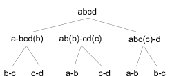
Figure 4: Example of Search Space

Obviously, when the regular expression gets complex, if such brute-force method is applied, the query optimization is costly. It is observed that the search space of possible query plans has overlapping space for subqueries. In the above example, state $a-bcd(b)$ and state $abc(c)-d$ share the same search space $b-c$. Then the direction of $b-c$ will be determined twice. Based on this observation, we propose a dynamic programming algorithm for query optimization for regular expression. To simplify the discussion, we will discuss the processing of the regular expression with only simple clause with at most one concentration operation in a closure without recursion closure.

At first, the operations in a regular expression $E$ is modeled as an operation graph $G_{E}$ based on their adjacent relationship. Each operation corresponds to a vertex in the operation graph. If two operations are adjacent, an edge is added to their corresponding vertices in the operation graph.

Each clause $C$ in $E$ corresponds to a subgraph $G_{C}$ in the $G_{E}$. Each possible query plan in $E$ corresponds to a spanning tree in $G_{E}$. Similarly, each possible query plan for a clause $C$ corresponds to a spanning tree in $G_{C}$. Note the that this problem cannot be solved trivially as minimal spanning tree because the cost of the query plan corresponding to a spanning tree is not the sum of the cost of each edge. The recursion function of the dynamic programming is as follows where $Cost_{G_{c}-u}$ represents the sum of cost of the optimal plans for the clauses corresponding to $Cost_{G_{c}-u}$ and $Cost(u|G_{c})$ is the optimal cost of operator corresponding to $u$ after the optimal query plan for $G_{c}$ has been executed. $Cost(u|G_{c})$ can be computed from two possible direction of $u$ after the processing of $G_{c}$.

$$Cost_{G_{C}}=min_{u\in V_{G_{c}}}\{Cost_{G_{c}-u}+Cost(u|G_{c})\}$$

Based the recursion function, the pseudo-code of query optimization is shown in Algorithm 7. During processing, a hash table with the key as the bitmap for the vertices in the subgraph is maintained to map the subset of vertices of $G_{E}$ to their corresponding optimal cost. A hash table $R$ maps each subset of vertices $V$ of $G_{E}$ to the chosen operator as the last operator for processing the induced graph $G_{E}[V]$, which consists of $V$ and all edges with endpoints contained in $T$.

Algorithm 7 Optimization($E$)

  construct $G_{E}$ for $E$

  $\mathbb{S}=\varnothing$

  for each node $v\in V_{G_{E}}$ do

     compute the cost $cost_{v}$ of $v$

     $H[v]$=$cost_{v}$

     add $v$ to $\mathbb{S}$

  for i=2 to $|V_{G_{E}}|$ do

     $\mathbb{S}^{\prime}$=$\mathbb{S}$

     $\mathbb{S}$=$\varnothing$

     for each $V$ in $\mathbb{S}^{\prime}$ do

        for each $v$ in $V$ do

           for each ($v$, $u$) in $V_{G_{E}}$ do

              if $u\notin V$ then

                 add $V\bigcup\{v\}$ to $\mathbb{S}$

     for each $V$ in $\mathbb{S}$ do

        $H[V]$=$\infty$

        for each $v$ in $V$ do

           $temp$=$H[V-\{v\}]$+$Cost(v|G_{E}[V])$

           if $temp<H[V]$ then

              $H[V]$ = $temp$

              $R[V]$ = $O_{v}$

  $V=V_{G_{E}}$

  for $i$=1 to $|V_{G_{E}}|$ do

     add $R[V]$ to the first of $L$

     $V=V-\{R[V]\}$

  return $L$

We use an example to illustrate the process of the algorithm.

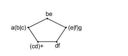
Figure 5: The Operation Graph

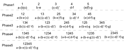
Figure 6: The Search Space of Dynamic Programming

Example 5

During the optimization for query $a(be|(cd)^{+}f)g$, the basic operator include (1) $a(b|c)$; (2)$be$; (3)$(cd)^{+}$; (4)$df$; (5)$(e|f)g$. The operation graph is shown in Figure 5. In this figure, each node represents an operator, and each edge represents the concatenation relationship between its vertices. The states and phases of the dynamic programming is shown in Figure 6, where each state corresponds to a set of nodes in the operation graph and a subquery. For each state, the node set is represented as a list of numbers in the above and the corresponding subquery is the string below the numbers. To distinguish the concentration of two adjacent symbols and adjacent symbols without relationship, we use ‘-’ to represent concentration.

The states of higher-level phases are generated with related lower-level phases. The plan corresponding to the state for subquery $a-(b-e|(c-d)^{+}f)$ is chosen from four possible plans ({$E_{1}$=$a(b|(cd)^{+}f)$}, $E_{1}(b)-e$) ({$E_{2}$=$be|(cd)^{+}f$}, $a-E_{2}(b,c)$) ({$E_{3}$=$a(be|c)$,$E_{4}$=$df$}, $(E_{3}(c)-E_{4}(d))^{+}$) ({$E_{5}$=$a(be|(cd)^{+})$}, $E_{5}(d)-f$). In each binary, the first entry is the subqueries to be executed first the plan corresponding to which have been computed and the second entry is the last operator whose execution direction is determined in this step.

In the worst case, the time complexity of Algorithm 7 is O($|V|2^{|V|}$), which requires to enumerate all possible combination of vertices. Such case happens when the $G_{E}$ is a clique. Fortunately, such case will exist only when $E=a(b_{1}|b_{2}|\cdots|b_{n})$. When there is not ‘$|$’ in the regular expression, $R_{E}$ degenerates to a line and the time complexity is O($|V|^{2}$).

To accelerate the query optimization, the clause $a_{1}|a_{2}\cdots|a_{n}$, where each $a_{i}$ is a label, is considered as single label during the processing.

The difficulty in the optimization of recursive closure is that for large graph. Only local statistic information is maintained and insufficient for recursive closure, which may match paths with various lengths. Note that according to our cost model, if a clause is in a closure, except the first and the last operator in the clause, the operators will not affected by the operators outside the clause. Based on the independent assumption in the estimation strategy, for the operator ClosureLink($a$, $b$), its cost is proportional with $size^{\prime}(a)$ which is the only operator affected by other operators. Additionally, only a share of candidates corresponding to the head and tail of the clause in closure will be affected by the previous operators. For example, for the query $a(bcd)^{+}$, if the subquery $ab$ is executed before the closure, the execution number of the operation matching the path $bcd$ will be not only determined by the number of $b$ in the results matching $ab$ but also affected by the number of $b$ neighbors of $d$ nodes.

Therefore, for the optimization of closure in a query, we generate the query plan for the clause in the closure before the optimization for the whole query. Such plan is used as an operator without the modification during the optimization for the whole query. When a query has multiple levels of recursion closure, such closures are process from inner to outer recursion.

For example, for the query $a(b(cdf)^{+}e)^{+}g$, the query plan for $cdf$ is generated at first. Then the query plan for $b(cdf)^{+}e$ is generated with the plan for $cdf$ as an operator. Similarity, during the optimization of the whole query, $b(cdf)^{+}e$ is considered as an operator.

6 Experiments

To verify the efficiency of the proposed approaches, we conduct extensive experiments. In this section, we propose the experimental results and analysis.

6.1 Experimental Setting

We conduct the experiments on a cluster consisting of 32 servers. Each server has 72GB DDR3 RAM and two 2.67 GHz Intel Xeon X5660 CPU. Each CPU has 6 cores and 12 threads. The network adapters is Broadcom BCN5709C NetXtreme GigE. Each server’s operating system is Windows Server 2008 R2 Enterprise with service pack 1. Our code was written with C# and compiled by .NET Framework 4.5. All the experiments are run on Microsoft GraphEngine .

We use both real and synthetic data to test our system. We design three kinds of queries for each graph to test the performance of algorithms with various kinds of queries. The first type of the queries (Hand) is generated by randomly handwriting some complicated regular expression as the query pattern with specific semantics. To test the performance for the queries with at least one result, the second type of the queries (BFS) is generated by BFS traversal from a randomly chosen node, and the first $N$ nodes are kept as the query patent. To test the performance for queries with complex structure and various regular expression features, the last type of the queries (Random) is generated by randomly adding labels and wildcards in the regular expression.

Each label in the regular expression is chosen from the label set of the graph. For each kind of queries, we generate five kinds of regular expressions with lengths 5, 10, 15, 20, 25 respectively, and generate five different regular expression as query pattern for each length. For each query, we execute 10 times and record its average execution time.

6.2 Experimental Results

6.2.1 Experimental Results on Real Data

For real data, We use freebase data set. It is a large collaborative knowledge base consisting of data composed mainly by its community members. This graph obeys the power law [3]. It contains 83,409,054 nodes and 293,351,870 edges. We use the type of each subject as an element of our label collection. This graph has totally 16,524 labels. The loading time of freebase is 34,464ms.

The Impact on Query Length To test the impact of query length, we vary the length from 5 to 25 and the results are shown in Figure 7(a). From the results, the query time increases with the increase of the length of the regular expression approximately. The instable cases are caused by the variety in the structure of randomly generated queries.

In the case of the same length of the regular expression, different regular expression query has different execution time. The reasons are as follows. On the one hand, longer regular expression causes more logical operators, and more physical operators will be generated. As the result, more intermediate result sets will be loaded in the memory, and more join operations are performed.

On the other hand, each regular expression is different from other regular expressions with the same length, the labels and the wildcards are not the same in each regular expressions. Therefore, in the case of the same length of the regular expression, the execution time are not the same. Another observation is that the process time of Random is less than Hand and BFS in the case of same length of the regular expression. The reasons are in two aspects. On the one hand, the degree of the real graph obeys in power low, the graph is a sparse graph, and most of the nodes have little degrees. On the other hand, the intermediate result set of the logical operators composed of random labels may not exist.

The Effectiveness of Query Optimization To verify the contribution of our query optimization strategy, we generate three regular expressions, each of which has complex structure, as the test queries and 10 query plans randomly for each query and compare the processing time with the optimized query plan. The experimental results are shown in Table IX. From the experimental results, the optimized query plan outperforms the average running time significantly and is near to or smaller than the minimal running time of randomly generated query plans. Additionally, the effectiveness of query optimization is significant when when the processing time of queries is long. This shows that our query optimization strategy could effectively avoid the worst case and is suitable for the queries whose processing time is relative long.

TABLE IX: The Results for Query Optimization

Query	Op	Max	Min	Avg
$md^{+}(e|h)(kf)^{+}(b|l)(oj)^{+}(c|i)(ga)^{+}n$	1593	9016	730	3720
$fg(cj)^{+}(b|i)(he)^{+}da$	120	183	100	133
$v(b|l)(oj)^{+}(p|s)(yu)^{+}(t|z)x^{+}(ga)^{+}w$	2036	8146	2168	5234

6.2.2 Experimental Result on Synthetic Data

To verity the performance of our matching algorithms deeply, our approach is further evaluated on a set of synthetic graphs generated using RMAT [4] with node count, average degree and label number as the parameter. The default node count and average degree are 1024M and 64, respectively. The labels of the graph are from a set of persons with 5,163 labels. The whole label set is used by default.

Scalability To test the scalability, we vary the node number from 32M to 1024M. The loading time is shown in Table X. From the results, we observe that even when the graph size scales to 1B, it can be loaded in our system within a few thousands of milliseconds.

TABLE X: Load Time for Synthetic Data

Node Number(M)	32	64	128	256	512	1024
Load Time(ms)	3067	3824	3660	5105	5775	8199

The scalable experimental results are shown in Figure 7(b). From the results, the running time increase sublinearly with the number of nodes, as show that our matching algorithms scales well as graph grows large.

The Impact of Query Length To test the impact of query length, we verify the query length from 5 to 20. Experimental results are shown in Figure 7(c). From the experimental results, the longer regular expression is, the more response time is. It is due to more operators caused by longer regular expression.

The Impact of Graph Density To test the impact of graph density, we vary the average degree from 4 to 64. The results are shown in Figure 7(d). From the results, the response time increases linearly with the average degree. This is caused by the increases in the size of intermediate results to handle. That is, with the increase of the average degree, the interconnections within the nodes increase and as the result, the number of intermediate results increases.

The Impact of Label Number To test the impact of label number, we choose 100%, 50%, 25%, 12.50%, 6.23% labels from the whole label set to generate label sets with 5163, 2581, 1290, 645, 322 labels. The experimental results are shown in Figure 7(e). From the results, the running time decreases significantly from the label number. The reason is that when label number increases, the number of nodes with the same label gets small and the number of nodes to be handled by the query decreases correspondingly.

Speedup To test the speedup of our system, we vary the machine number from 1 to 32 and the experimental results are shown in Figure 7(f). From the results, when the machine number increase from 1 to 8, the running time decreases significantly. While when the machine number gets larger, the running time increases slightly. This is because when the machine number is small, the time of cluster maintenance is relative small. Thus the acceleration effect of increasing machine number is significant. As a comparison, when the machine number gets large, the load of cluster maintenance is heavy and in such case, the running time gets slow. This shows that our systems could achieve high performance with more number of machines.

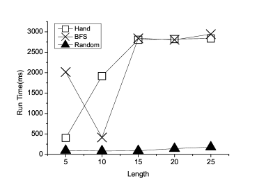
(a) The Impact of Query Length (Real Data)

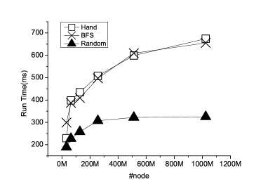
(b) The Impact of Node Number (Synthetic Data)

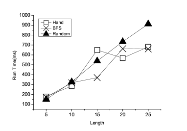
(c) The Impact of Query Length (Synthetic Data)

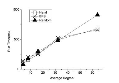
(d) The Impact of Graph Density (Synthetic Data)

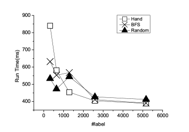
(e) The Impact of Label Number (Synthetic Data)

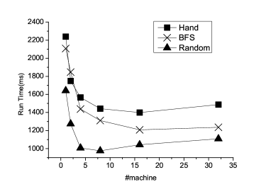
(f) Speedup (Synthetic Data)

Figure 7: Experimental Results

7 Related Work

Since regular expression is a powerful form for query requirement description on sequences, structural queries with regular expression on data with complex structures,such as XML data and graphs, have been studied.

Some work focus on the expressive power of query language. [2] surveys various syntax and semantics regular expression queries on graphs. nSPARQL [13] embed regular expression into SPARQL. Different from these work, our concern is the efficiency and scalability. [DBLP:conf/semweb/KostylevR0V15] studied the difficulty of the evaluation, containment and subsumption with SparQL with embedded regular expressions.

Due to the importance, the regular expression path query (RPQ for brief) processing on large graphs have be studied. Some algorithms have been proposed to process RPQ efficiently. [6] uses regular expression to describe the relationship between the vertices in the graph pattern. It allows path queries with regular expressions formed with edge-labels. An index with size O($|V|^{2}$) is used for query processing, which is not suitable for large graphs. Additionally, the regular expression in [6] considers neither recursion of expressions nor ‘$|$’. [11] processes RPQ queries by traversal and uses rare labels to optimize the RPQ query processing. [8] studies the processing of RPQ based reachability queries, which contain Kleene closure. It processes queries by translating the query graph into relational operators including scans, projections and joins. The label-based index for reachability queries is also proposed to accelerate query processing. This approach in only suitable the RPQs with closure on single label instead of a clause. [17] processes RPQ by translating RPQs into recursion SQL queries. Waveguide [18] builds a cost-based optimizer for SPARQL queries with regular expression. It generate a query plan as the combination of finite automatas for a RPQ. The RPQ is processed by graph traversal guided by the query plan. [15] the approximate matching and relaxation of conjunctive regular path queries by introducing two new operators for flexible query processing.

All these algorithms aim to process RPQ on single machine without parallel paradigm. The scalability is limited. Additionally, the expressive power of the languages used by some approaches is limited. Different from these work, our system adopts parallel mechanism to process queries in full regular expression syntax on billion-nodes graphs.

Horton+ [14] adopts a parallel platform to process RPQ on graphs. It also decomposes the query into segments and joins their results.

8 Conclusion

In this paper, we study the problem of regular expression (RE) matching on large graphs, which is to retrieve pairs of vertices in the graph with the labels in the path between them satisfying the constraint of the RE in the query. We propose the methods to process the RE query on large graphs with the index sublinear to the graph size. To obtain the efficient query plan for regular expression query processing, we design the query optimization strategy based on the cost model in absence of the global structural statistical information for the graph. To process the RE queries on web-scale graphs, we also develop the parallel processing algorithm independency to the distribution of data with two simple network primitives. Experimental results demonstrate that our system can scale to billion-node graphs.

As the future work, we plan to study two problems. One is the efficient processing methods with the regular expression with wildcard, especially with the wildcard in the closure. The other is to study the efficient matching algorithm for graph patterns with regular expressions embedded in them.

References

- [1] Facebook: One social graph to rule them all? CBS News. July 11, 2010.
- [2] R. Angles, M. Arenas, P. Barceló, A. Hogan, J. L. Reutter, and D. Vrgoc. Foundations of modern query languages for graph databases. ACM Comput. Surv., 50(5):68:1–68:40, 2017.
- [3] D. Chakrabarti and C. Faloutsos. Graph Mining: Laws, Tools, and Case Studies. Synthesis Lectures on Data Mining and Knowledge Discovery. Morgan & Claypool Publishers, 2012.
- [4] D. Chakrabarti, Y. Zhan, and C. Faloutsos. R-MAT: A recursive model for graph mining. In SDM, pages 442–446, 2004.
- [5] P. E. C. Compeau, P. A. Pevzner, and G. Tesler. How to apply de bruijn graphs to genome assembly. Nature Biotechnology, 29.
- [6] W. Fan, J. Li, S. Ma, N. Tang, and Y. Wu. Adding regular expressions to graph reachability and pattern queries. In ICDE, pages 39–50, 2011.
- [7] G. H. L. Fletcher, J. Peters, and A. Poulovassilis. Efficient regular path query evaluation using path indexes. In EDBT, 2016.
- [8] A. Gubichev, S. J. Bedathur, and S. Seufert. Sparqling kleene: fast property paths in RDF-3X. In First International Workshop on Graph Data Management Experiences and Systems, GRADES 2013, co-loated with SIGMOD/PODS 2013, New York, NY, USA, June 24, 2013, page 14, 2013.
- [9] H. Hosoya and B. C. Pierce. Regular expression pattern matching for xml. In POPL, pages 67–80, 2001.
- [10] H. Hosoya and B. C. Pierce. Xduce: A statically typed xml processing language. ACM Trans. Internet Techn., 3(2):117–148, 2003.
- [11] A. Koschmieder and U. Leser. Regular path queries on large graphs. In Scientific and Statistical Database Management - 24th International Conference, SSDBM 2012, Chania, Crete, Greece, June 25-27, 2012. Proceedings, pages 177–194, 2012.
- [12] Q. Li and B. Moon. Indexing and querying xml data for regular path expressions. In VLDB, pages 361–370, 2001.
- [13] J. Pérez, M. Arenas, and C. Gutierrez. nsparql: A navigational language for RDF. J. Web Sem., 8(4):255–270, 2010.
- [14] M. Sarwat, S. Elnikety, Y. He, and M. F. Mokbel. Horton+: A distributed system for processing declarative reachability queries over partitioned graphs. PVLDB, 6(14):1918–1929, 2013.
- [15] P. Selmer, A. Poulovassilis, and P. T. Wood. Implementing flexible operators for regular path queries. In Proceedings of the Workshops of the EDBT/ICDT 2015 Joint Conference (EDBT/ICDT), Brussels, Belgium, March 27th, 2015., pages 149–156, 2015.
- [16] Z. Sun, H. Wang, H. Wang, B. Shao, and J. Li. Efficient subgraph matching on billion node graphs. PVLDB, 5(9):788–799, 2012.
- [17] N. Yakovets, P. Godfrey, and J. Gryz. Evaluation of SPARQL property paths via recursive SQL. In Proceedings of the 7th Alberto Mendelzon International Workshop on Foundations of Data Management, Puebla/Cholula, Mexico, May 21-23, 2013., 2013.
- [18] N. Yakovets, P. Godfrey, and J. Gryz. WAVEGUIDE: evaluating SPARQL property path queries. In EDBT, 2015.
- [19] N. Yakovets, P. Godfrey, and J. Gryz. Query planning for evaluating SPARQL property paths. In SIGMOD, 2016.
- [20] K. Zeng, J. Yang, H. Wang, B. Shao, and Z. Wang. A distributed graph engine for web scale RDF data. PVLDB, 6(4):265–276, 2013.
- [21] Q. Zhang, W. Zheng, and M. R. Lyu. Flow-augmented call graph: A new foundation for taming API complexity. In FASE, pages 386–400, 2011.