The evolution and dependence of the local mass-metallicity relation

Abstract

We present a sample of 86,111 star-forming galaxies (SFGs) selected from the catalogue of the MPA-JHU emission-line measurements for SDSS DR7 to investigate the evolution of mass-metallicity (MZ) relation. We find that: under the $\rm log(L_{H\alpha})>41.0$ threshold, the $0.04<z\leqslant 0.06$ SFGs with $9.2<$ log($M_{\star}/M_{\sun})<9.5$ have always higher metallicities ($\sim 0.1$ dex) than the $0.10<z<0.12$ SFGs by using the closely-matched control sample method; under the $\rm log(L_{[\rm O~{}\sc{III}]})>39.7$ threshold, the $0.04<z\leqslant 0.06$ SFGs with $9.2<$ log($M_{\star}/M_{\sun})<9.5$ do not exhibit the evolution of the MZ relation, in contrast to the $0.10<z<0.12$ SFGs. We find that the metallicity tends to be lower in galaxies with a higher concentration, higher Sérsic index, or higher SFR. In addition, we can see that the stellar mass and metallicity usually present higher in galaxies with a higher $D_{n}4000$ or higher log(N/O) ratio. Moreover, we present the two galaxy populations with log($M_{\star}/M_{\sun}$) below $10.0$ or greater than $10.5$ in the MZ relation, showing clearly an anticorrelation and a positive correlation between specific star formation rate and 12+log(O/H).

1 INTRODUCTION

The connection between stellar mass ($M_{\star}$) and gas-phase oxygen abundance (metallicity, Z) is one of the most fundamental relations established in the galaxy formation and evolution. The mass-metallicity (MZ) relation was first shown by Lequeux et al. (1979), and later observations confirmed it with a larger sample from the Sloan Digital Sky Survey (SDSS; Tremonti et al. 2004). Beyond the local universe, the MZ relation has been observed to extend out to $z\sim 3.5$, and the metallicity decreases with increasing redshift at a given stellar mass (Erb et al. 2006; Maiolino et al. 2008; Troncoso et al. 2014; Sanders et al. 2015). With regard to the origin of the MZ relation, physical explanations generally invoke an equilibrium between metal-enriched gas outflows and pristine gas inflows (Mannucci et al. 2010; Lara-López et al. 2010; Brown et al. 2018), therefore the change from the balance may be a tracer of understanding these mechanisms.

Some studies demonstrated the star formation rate (SFR) dependence of MZ relations (Ellison et al. 2008; Mannucci et al. 2010; Lara-López et al. 2010; Andrews & Martini 2013). The dependence of the MZ relation on SFR originated from the work of Ellison et al. (2008), and Mannucci et al. (2010) and Lara-López et al. (2010) found almost simultaneously a tight relationship among SFR, stellar mass, and metallicity for z$\sim 0.1$ star-forming galaxies (SFGs), and concluded that the $\rm M-\rm Z-SFR$ relation is invariant at $z<2.5$ and $z<3.5$, respectively. In addition, several studies reported that SFGs at $z\sim 1-3$ do not show any evidence for the redshift evolution of $\rm M-SFR-Z$ relation (Christensen et al. 2012; Wuyts et al. 2012, 2016; Belli et al. 2013; Henry et al. 2013; Stott et al. 2013; Maier et al. 2014; Yabe et al. 2015; Hunt et al. 2016; Sanders et al. 2018).

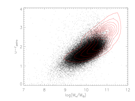
Figure 1: The stellar mass and u-r colour diagram. Our SFG sample occupys the blue sequence (black dots), and the red contours represent the distribution of the whole SDSS DR7 sample.

Moreover, Salim et al. (2014) studied the relation between metallicity and specific star formation rate (sSFR=SFR/$M_{\star}$) in distinct mass bins by analyzing the SDSS data, and found a significant correlation yet fairly weaker than that shown by Mannucci et al. (2010). Collecting 1381 field galaxies at $0.5\leqslant z\leqslant 0.7$ from deep spectroscopic survey, Guo et al. (2016) found that the dependence of MZ relations on SFR is weaker than that presented in local galaxies.

Utilising the CALIFA data to study the MZ relation, Sánchez et al. (2013) did not find a correlation between the MZ relation and SFR. Recently, Barrera-Ballesteros et al. (2017) presented the integrated MZ relation with more than 1700 MaNGA SFGs, and found no dependence of the MZ relation on SFR. Besides, many other literatures presented that galaxies at $z\sim 1-3$ do not trace the predictions of the $z\sim 0$ FMR, indicating an evolving $\rm M-SFR-Z$ relation (Cullen et al. 2014; Yabe et al. 2014; Zahid et al. 2014; Wuyts et al. 2014; Sanders et al. 2015, 2018; Salim et al. 2015; Kashino et al. 2017).

Since many studies mentioned above focus on the SFR dependence of MZ relations, we restrain the stellar mass and SFR to explore the redshift evolution of the MZ relaition. In addition, we revisit the evolution of the MZ relation and investigate the MZ relation with the Sérsic index, concentration index, and $D_{n}4000$. The paper is organized as follow. In Section 2, we show the SFG sample and various data. We explore the evolution of the MZ relation, and investigate the dependence and scatter of the MZ relation with the Sérsic index, concentration index, SFR, sSFR, log(N/O), and $D_{n}4000$ in Section 3. In Section 4, the results and conclusions are summarized. We adopt $H_{0}=70~{}\rm km~{}s^{-1}~{}Mpc^{-1}$, $\Omega_{M}=0.3$, and $\Omega_{\Lambda}=0.7$.

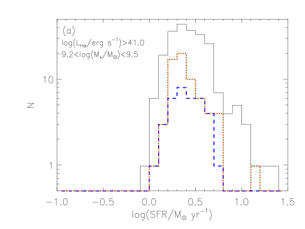
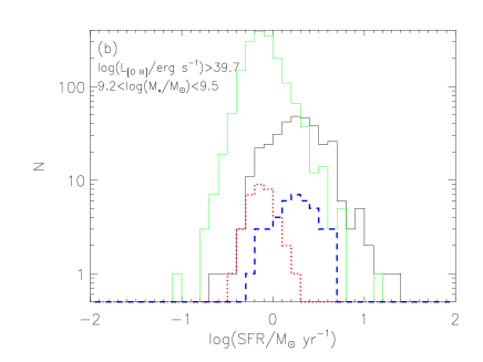
Figure 2: Comparison of the SFR distributions of different sample SFGs with $9.2<$log$(M_{\star}/M_{\sun})<9.5$. Panel(a) for log(L${}_{\rm H\alpha})>41.0$. Panel(b) for log(L${}_{\rm[OIII]})>39.7$. The green and black lines are the SFR distributions of SFGs at $0.04<z\leqslant 0.06$ and $0.10<z<0.12$, respectively. The red dotted (blue dashed) lines show the SFR distributions of control samples, which have the same SFR distribution as the SFGs at $0.04<z\leqslant 0.06$ ($0.10<z<0.12$), and come randomly from the SFGs at $0.10<z<0.12$ ($0.04<z\leqslant 0.06$), respectively.

Table 1: Summary of the evolution of the MZ relations for different sample SFGs.

	low/high z	CSs	log(SFR)		$p_{\rm null}(\%)$	log($M_{\star}$)		$p_{\rm null}(\%)$	$12+\rm log(O/H)$		$p_{\rm null}(\%)$
			$M_{\sun}/yr^{-1}$			$M_{\sun}$
(1)	(2)	(3)	(4)	(5)	(6)	(7)	(8)	(9)	(10)	(11)	(12)
$\rm log(L_{H\alpha})>41.0$	66	66	$0.36\pm 0.19$	$0.37\pm 0.19$	54	$9.40\pm 0.09$	$9.41\pm 0.08$	83	$8.71\pm 0.11$	$8.57\pm 0.12$	$4.6\times 10^{-5}$
	225	35	$0.42\pm 0.32$	$0.37\pm 0.17$	53	$9.42\pm 0.08$	$9.40\pm 0.09$	85	$8.60\pm 0.13$	$8.71\pm 0.09$	0.0296
$\rm log(L_{[\rm O~{}\sc{III}]})>39.7$	1714	35	$-0.11\pm 0.21$	$-0.15\pm 0.15$	74	$9.35\pm 0.09$	$9.39\pm 0.09$	22	$8.76\pm 0.10$	$8.78\pm 0.11$	51
	338	41	$0.27\pm 0.36$	$0.22\pm 0.24$	65	$9.40\pm 0.08$	$9.41\pm 0.09$	68	$8.66\pm 0.14$	$8.78\pm 0.11$	0.00142

Note: Cols.(1): The different samples. Cols.(2) and (3) are the number of the samples of $0.04<z\leqslant 0.06$ (the lower redshift) or $0.10<z<0.12$ (the higher redshift) and their corresponding control samples(CSs). Cols.(4), (7), and (10): the median value of log(SFR), log($M_{\star}$), and 12+log(O/H), respectively, which comes from the lower (higher) redshift sample. Cols.(5), (8), and (11): the median value of log(SFR), log($M_{\star}$), and 12+log(O/H), respectively, which comes from their corresponding control samples (CSs). Cols.(6), (9), and (12): the probabilities for the null hypothesis that the two distributions are drawn randomly from the same population.

2 THE DATA

The sample in this study is selected from the catalogue of the SDSS Data Release 7 (DR7; Abazajian et al. 2009). We utilise measurements of emission line fluxes, SFRs, and stellar masses, which are publicly available from the catalogue of Max Planck Institute for Astrophysics$-$John Hopkins University (MPA-JHU) SDSS DR7 release. To avoid the bias of the MZ relation from the aperture effect (Kewley, Jansen & Geller 2005) and the selection effect of the metallicity evolution (Zahid et al. 2013; Wu et al. 2016), these galaxies are required to have the lower and upper redshift limits of 0.04 and 0.12. Also, the covering fractions are $>20\%$ of all galaxy fluxes, which are calculated from the r band fiber and Petrosian magnitudes. According to the BPT diagram (Baldwin et al. 1981; Kauffmann et al. 2003a; Kewley et al. 2006), we obtain the SFGs from the above sample by using the equation (log([O III]$/\rm H\beta)<0.61/[log([\rm N~{}\sc{II}]/\rm H\alpha)-0.05]+1.3$) of Kauffmann et al. (2003a), forming an initial sample of 136,964 galaxies.

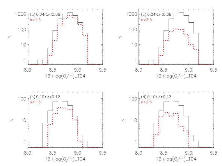
Figure 3: Comparison of the metallicity distributions of different Sérsic index SFG samples with $9.2<$log$(M_{\star}/M_{\sun})<9.5$. The black line of Fig. 3(a) (Fig. 3(b)) is the metallicity distribution of $0.04<z\leqslant 0.06$ ($0.10<z<0.12$) SFGs with $9.2<$log$(M_{\star}/M_{\sun})<9.5$. Fig. 3(a) (Fig. 3(b)) has the same black line as Fig. 3(c) (Fig. 3(d)). The red dotted line of Fig. 3(a) (Fig. 3(c)) is the metallicity distribution of $0.4<z\leqslant 0.06$ SFGs with $n<1.5$ ($n>2.5$) and $9.2<$log$(M_{\star}/M_{\sun})<9.5$. The red dotted line of Fig. 3(b) (Fig. 3(d)) is the metallicity distribution of $0.10<z<0.12$ SFGs with $n<1.5$ ($n>2.5$) and $9.2<$log$(M_{\star}/M_{\sun})<9.5$.

We use the emission line fluxes of [O II] $\lambda\lambda 3727,3729$, H$\beta$, [O III] $\lambda\lambda 4959,5007$, H$\alpha$, and [N II]  $\lambda 6584$ to analyze the MZ relation. The signal-to-noise ratio (S/N) cut of [O III] $\lambda 5007$ may bias the MZ relation, due to that this emission line often appears in high metallicity galaxies (Foster et al. 2012). Therefore, we choose the SFGs with S/N $>3$ for H$\beta$, H$\alpha$, [O II] $\lambda\lambda 3727,3729$, and [N II]  $\lambda 6584$. Since an SFR FLAG keyword shows the status of the SFR measurements, the keyword of $0$ is required. To break the degeneracy between the upper and lower branch $R_{23}$ solutions, we choose the SFGs with log([N II] $\lambda 6584$/[O II]$\lambda 3727$)$>-1.2$ in our sample (Kewley & Ellison 2008). In fact, we find that the N2O2 ratio excludes only one SFG from the above sample, so it does not introduce a selection bias to our final sample. Finally, we obtain the final sample of 86,111 SFGs.

Regarding SFRs and $M_{\star}$, we use a Chabrier (2003) initial mass function (IMF) to correct them assumed a Kroupa (2001) IMF by dividing it by 1.06. To study the MZ relation, we use the Petrosian half-light radii $R_{50}$ and $R_{90}$, which are the radius enclosing $50\%$ and $90\%$ of the Petrosian flux, respectively (Shen et al. 2003), and are from the New York University Value-Added Galaxy Catalogue (NYU-VAGC; Blanton et al. 2005). With regard to the Petrosian flux, please see Section 2.1 of Shen et al. (2003). Provided the radii $R_{50}$ and $R_{90}$, the concentration index of a galaxy is defined as $c=R_{90}$/$R_{50}$, which is related to galaxy morphological types. Also, we introduce a $D_{n}4000$ index to study the MZ relation. The index is defined as a flux ratio in two spectral windows, which is close to the 4000Å break (Balogh et al. 1999): 3850-3950Å and 4000-4100Å (Zahid & Geller 2017). The index increases with the stellar population age (Kauffmann et al. 2003a; Zahid et al. 2015). In addition, we adopt $n$ to represent the Sérsic index, obtained from the NYU group (Zahid & Geller 2017). The Sérsic index ($n$) ranges are from $0$ to $5.9$. For quiescent galaxies, Zahid & Geller (2017) showed that galaxies with higher $D_{n}4000$ often have larger Sérsic indexes at a given stellar mass. Due to the two indexes(c and n) estimated from the NYU-VAGC, we cross-match it with the MPA-JHU SDSS DR7 catalogue within $2^{\prime\prime}$, and obtain 81,125 SFGs. In this paper, we will utilise a sample of 86,111 SFGs if the two indexes are not involved in our studies.

In Figure 1, we present the diagram of stellar mass and u-r colour (from Petrosian magnitudes). The red contours of Figure 1 are the distribution of 862,079 galaxy sample, which comes from the cross-match of the NYU-VAGC and MPA-JHU SDSS DR7 catalogues. Our sample of 86,111 SFGs is shown with the black dots in Figure 1. From Figure 1, we find that all SFGs of our sample are almost the late-type galaxy. For the morphologies of Sérsic indexes, we use $n>2.5$ and $n<1.5$ to represent the spheroid-dominated and disk-dominated galaxies, respectively (Maier 2009). The concentration indexes $c\geqslant 2.86$ and $c<2.86$ are used to separate early-type and late-type galaxies (Nakamura et al. 2003; Shen et al. 2003). In addtion, we show that these galaxies with $n>2.5$ or $c>2.86$ have lower matallicities compared to the late-type galaxies in Figures 3(c) and 3(d) or Figures 4(c) and 4(d). This is not consistent with that early-type galaxies generally have higher stellar metallicity than the late-type galaxies with larger difference in lower masses (Peng et al. 2015). In fact, these galaxies are likely to be compact SFGs which usually show lower gas metallcity than the normal SFGs (Hoopes et al. 2007). In this paper, the two indexes (c and n) only represent the galaxy structure properties.

In this paper, we use the $R_{23}$ method to estimate oxygen abundances of SFGs (Pilyugin et al. 2006, 2010; Wu & Zhang 2013), and adopt the calibration of T04. In addition to the T04 method, we use the five methods of metallicity estimators, for instance, Dopita 2016 (D16), Pettini & Pagel 2004 (PP04-O3N2 and PP04-N2), Zaritsky, Kennicutt & Huchra 1994 (Z94), and Sanders et al. 2018 (Sander18).

3 Results

In this section, we first explore the evolution of the MZ relation using a control sample method under the emission line luminosity limits for log(H$\alpha$) and log($[\rm O~{}\sc{III}]$) and using comparison of metallicity differences under the different galaxy morphologies. Then we investigate the dependence of MZ relations of $0.04<z\leqslant 0.06$ and $0.10<z<0.12$ SFGs on the Sérsic index, concentration index, SFR, sSFR, log(N/O), and $D_{n}4000$. Finally, we study the scatter of MZ relations with different metallicity estimators, Sérsic index, and concentration index.

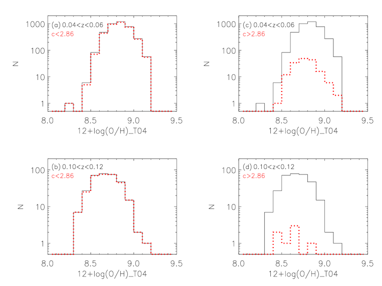
Figure 4: Comparison of the metallicity distributions of different concentration index SFG samples with $9.2<$log$(M_{\star}/M_{\sun})<9.5$. The black line of Fig. 4(a) (Fig. 4(b)) is the metallicity distribution of $0.04<z\leqslant 0.06$ ($0.10<z<0.12$) SFGs with $9.2<$log$(M_{\star}/M_{\sun})<9.5$. Fig. 4(a) (Fig. 4(b)) has the same black line as Fig. 4(c) (Fig. 4(d)). The red dotted line of Fig. 4(a) (Fig. 4(c)) is the metallicity distribution of $0.4<z\leqslant 0.06$ SFGs with $c<2.86$ ($c\geqslant 2.86$) and $9.2<$log$(M_{\star}/M_{\sun})<9.5$. The red dotted line of Fig. 4(b) (Fig. 4(d)) is the metallicity distribution of $0.10<z<0.12$ SFGs with $c<2.86$ ($c\geqslant 2.86$) and $9.2<$log$(M_{\star}/M_{\sun})<9.5$.

3.1 The evolution of the MZ relation

In the SDSS sample, Juneau et al. (2014) found an evolution of log($L_{\rm H\alpha}$) and $\rm log(L_{[\rm O~{}\sc{III}]}$). They got the observed limits of log($L_{\rm H\alpha}$) and $\rm log(L_{[\rm O~{}\sc{III}]}$), and presented an artificial evolution of the MZ relation. In the $0.04<z<0.12$ SDSS sample, Wu et al. (2016) also investigated and confirmed the redshift evolution of log($L_{\rm H\alpha}$), and $\rm log(L_{[\rm O~{}\sc{III}]}$). Wu et al. (2016) used the MZ relation of the $0.10<z<0.12$ subsample to correct the artificial evolution of MZ relations, and obtained the minimum luminosity limits of $\rm log(L_{H\alpha})>41.0$ and $\rm log(L_{[\rm O~{}\sc{III}]})>39.7$. In this article, we use a new method, the closely-matched control sample (Zhang, Kong & Cheng 2008), to check the evolution of the MZ relation. The control sample is constructed from the corresponding sample, which is matched in $M_{\star}$ and SFR. For instance, regarding the $0.04<z\leqslant 0.06$ SFG sample and its corresponding sample ($0.10<z<0.12$ SFGs), the control sample has the same SFR distribution as the SFGs at $0.04<z\leqslant 0.06$, and is randomly from the $0.10<z<0.12$ SFGs. In Wu et al. (2016), the metallicity difference of $\sim 0.15$ dex in the MZ relations happened at log($M_{\star}/M_{\sun})\sim 9.3$, so we choose $9.2<$ log$(M_{\star}/M_{\sun})<9.5$ as the stellar mass range matched. With regard to SFR matched, we employ the low (high) redshift range SFG sample and its corresponding control sample having the same SFR distribution. For comparision, all samples have the same stellar mass range matched of $9.2<$ log$(M_{\star}/M_{\sun})<9.5$.

In Figure 2(a), comparison of all samples at the two redshift ranges are based on the luminosity limit of $\rm log(L_{H\alpha})>41.0$. The green and black lines represent the distributions of SFRs of SFGs at $0.04<z\leqslant 0.06$ and $0.10<z<0.12$, respectively. The red dotted line shows the distribution of SFRs of the control sample, which has the same SFR distribution as the $0.04<z\leqslant 0.06$ SFGs, and comes randomely from the SFGs at $0.10<z<0.12$. The blue dashed line represents the distribution of SFRs of the control sample, which has the same SFR distribution as the $0.10<z<0.12$ SFG sample, and comes randomly from the SFGs at $0.04<z\leqslant 0.06$.

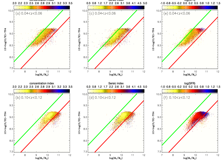
Figure 5: Comparison of the MZ relations of $0.04<z\leqslant 0.06$ and $0.10<z<0.12$ SFGs using the colour bars of the concentration index and Sérsic index, and SFR. The green and red lines are the diagnostic lines (is shown for reference) for comparing the MZ relations at different redshift ranges. The metallicity is estimated by the T04 method.

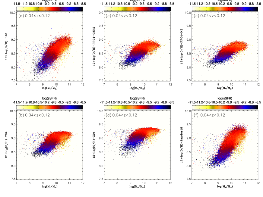
Figure 6: Comparison of the MZ relations of $0.04<z<0.12$ SFGs with the colour bars of sSFR for different metallicity estimators.

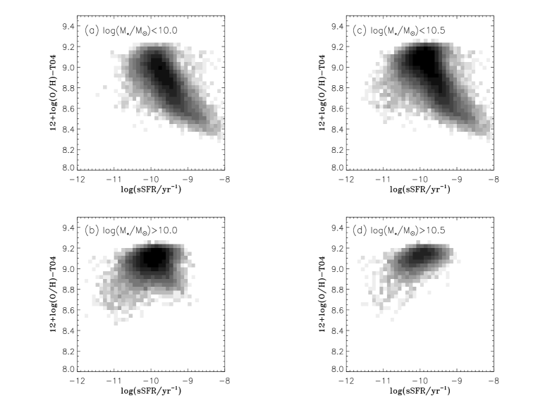
Figure 7: Comparison of the correlations between sSFR and metallicity of $0.04<z<0.12$ SFGs with different stellar mass ranges.

In Figure 2(b), we compare the SFR distributions of all samples for the two redshift ranges under the luminosity limit of $\rm log(L_{[\rm O~{}\sc{III}]})>39.7$. Following Figure 2(a), the green and black lines represent the SFR distributions of the SFGs at $0.04<z\leqslant 0.06$ and $0.10<z<0.12$, respectively. The red dotted line shows the SFR distribution of the control sample, which has the same SFR distribution as the $0.04<z\leqslant 0.06$ SFGs, and comes randomly from the SFGs at $0.10<z<0.12$. The blue dashed line represents the SFR distribution of the control sample, which has the same SFR distribution as the $0.10<z<0.12$ SFGs, and comes randomly from the SFGs at $0.04<z\leqslant 0.06$.

In Table 1, we show the summary of the evolution of MZ relations for the different samples. Under the luminosity threshold of $\rm log(L_{H\alpha})>41.0$ (also see Figure 2(a)), the median value of log(SFR), log($M_{\star}$), and 12+log(O/H) is $0.36\pm 0.19$, $9.40\pm 0.09$, and $8.71\pm 0.11$, respectively, in the $0.04<z\leqslant 0.06$ SFGs with $9.2<$ log$(M_{\star}/M_{\sun})<9.5$. The median value of log(SFR), log($M_{\star}$), and 12+log(O/H) is $0.37\pm 0.19$, $9.41\pm 0.08$, and $8.57\pm 0.12$, respectively, in their corresponding control sample with $9.2<$ log$(M_{\star}/M_{\sun})<9.5$. The median value of 12+log(O/H) in the $0.04<z\leqslant 0.06$ SFG sample is higher than the control sample by $\sim 0.1$ dex. The Kolmogorov-Smirnov (K-S) test of the SFR and log($M_{\star}$) distributions gives rather high probabilities of $54\%$ and $83\%$, showing the SFR and log($M_{\star}$) distributions between the two redshift ranges are drawn from the same population. The K-S test of the metallicity distribution yields a very low probability of $0.0046\%$, or equally a rejection at $99.9954\%$ confidence level, for the null hypotheses that the two distributions are drawn from the same population. These imply that the MZ relation evolution is found in the $0.04<z\leqslant 0.06$ SFG sample and its corresponding control sample with $9.2<$log$(M_{\star}/M_{\sun})<9.5$. In the $0.10<z\leqslant 0.12$ SFGs with $9.2<$log($M_{\star}/M_{\sun})<9.5$, the median value of log(SFR), log($M_{\star}$), and 12+log(O/H) is $0.42\pm 0.32$, $9.42\pm 0.08$, and $8.60\pm 0.13$, respectively. The median value of log(SFR), log($M_{\star}$), and 12+log(O/H) is $0.37\pm 0.17$, $9.40\pm 0.09$, and $8.71\pm 0.09$, respectively, in their corresponding control sample. Their probabilities for the two redshift range samples are $53\%$, $85\%$, and $0.0296\%$, respectively. These indicate that the two samples with the same distribution in SFR and mass show significant redshift evolution of MZ relation.

Under the luminosity threshold of $\rm log(L_{[\rm O~{}\sc{III}]})>39.7$ (also see Figure 2(b)), we follow the method of Figure 2(a). The median value of log(SFR), log($M_{\star}$), and 12+log(O/H) is $-0.11\pm 0.21$, $9.35\pm 0.09$, and $8.76\pm 0.10$, respectively, in the $0.04<z\leqslant 0.06$ SFGs with the same stellar mass range. The median value of log(SFR), log($M_{\star}$), and 12+log(O/H) is $-0.15\pm 0.15$, $9.39\pm 0.09$, and $8.78\pm 0.11$, respectively, in their corresponding control sample. The median value of 12+log(O/H) in the two samples has no difference ($\sim 0.0$ dex). The K-S test of the SFR, log($M_{\star}$), and metallicity distributions yields rather high probabilities of $74\%$, $22\%$, and $51\%$, showing that their distributions between the two samples are randomly drawn from the same parent population, and these indicate that the $0.04<z\leqslant 0.06$ sample and its corresponding control sample do not demonstrate the redshift evolution of the MZ relation. The $0.10<z<0.12$ SFGs with the same stellar mass range show that the median value of log(SFR), log($M_{\star}$), and 12+log(O/H) is $0.27\pm 0.36$, $9.40\pm 0.08$, $8.66\pm 0.14$, respectively. The median value of log(SFR), log($M_{\star}$), and 12+log(O/H) is $0.22\pm 0.24$, $9.41\pm 0.09$, and $8.78\pm 0.11$, respectively, in their corresponding control sample. The probabilities for the two redshift range samples are $65\%$, $68\%$, and $0.00142\%$. The K-S test shows the redshift evolution of the MZ relation.

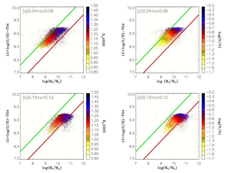
Figure 8: Comparison of the MZ relations of $0.04<z\leqslant 0.06$ and $0.10<z<0.12$ SFGs using the colour bars of $D_{n}4000$ and log(N/O), respectively. The green and red lines are the same diagnostic line as in Fig. 5.

From the above results, we find that the two different samples having higher SFRs (e.g. median(log(SFR))$>0.0$) based on the $0.04<z\leqslant 0.06$ and $0.10<z<0.12$ SFGs often have $\sim 0.1$ dex difference in metallicity, and that the two samples having lower SFRs (e.g. median(log(SFR))$<0.0$) based on the two redshift range SFGs usually have no significant difference in metallicity. In fact, these may originate from the different SFG samples selected different thresholds of emission line luminosities. In Figure 2(b), the control sample (red dotted lines) of the $0.04<z\leqslant 0.06$ SFGs with $9.2<$log$(M_{\star}/M_{\sun})<9.5$ almost comes from the $0.10<z<0.12$ SFGs with the same stellar mass range and the smallest SFRs. We can see that this sample comes mainly from the SFGs with $\rm 12+log(O/H)>8.7$ in Figure 4(b) of Wu et al. (2016, see the SFGs at $0.10<z<0.12$ (the red contour) and the luminosity threshold of $\rm log(L_{[\rm O~{}\sc{III}]})>39.7$ (the black line)). Although our sample is not just the same as the sample of Wu et al. (2016), both samples utilise the same luminosity threshold of $\rm log(L_{[\rm O~{}\sc{III}]})>39.7$. Due to the speciality of the sample, almost no evolution of the MZ relation is found in the SFGs with lower SFRs. Therefore, we speculate that the evolution of the MZ relation is clearly observed in the higher SFR SFGs.

In addition, we study the metallicity difference between the two redshift range samples with different galaxy morphologies. In Figures 3(a) and 3(b), we show the metallicity distributions of different SFGs with $9.2<$log$(M_{\star}/M_{\sun})<9.5$. The black line of Figure 3(a) (Figure 3(b)) is the metallicity distribution of $0.04<z\leqslant 0.06$ ($0.10<z<0.12$) SFGs with $9.2<$log$(M_{\star}/M_{\sun})<9.5$. The red dotted line of Figure 3(a) (Figure 3(b)) is the metallicity distribution of $0.04<z\leqslant 0.06$ ($0.10<z<0.12$) SFGs with $n<1.5$ and $9.2<$log($M_{\star}/M_{\sun})<9.5$. From Figures 3(a) and (b), we can see a significant difference of the metalicity distributions, showing that the lower redshift SFGs have higher metallicities than the higher redshift SFGs, and that the median metallicity is $8.85\pm 0.11$ and $8.72\pm 0.13$, respectively.

In Figures 3(c) and 3(d), the black lines are the metallicity distributions of $0.04<z\leqslant 0.06$ and $0.10<z<0.12$ SFGs with $9.2<$log$(M_{\star}/M_{\sun})<9.5$, respectively. Also, Figure 3(a) (Figure 3(b)) has the same black line as Figure 3(c) (Figure 3(d)). The red dotted line of Figure 3(c) (Figure 3(d)) is the metallicity distribution of $0.04<z\leqslant 0.06$ ($0.10<z<0.12$) SFGs with $n>2.5$ and $9.2<$log$(M_{\star}/M_{\sun})<9.5$. From Figures 3(c) and 3(d), a clear difference of the metalicity distributions is presented, showing that the lower redshift SFGs have higher metallicities than the higher redshift SFGs, and that the median metallicity is $8.78\pm 0.12$ and $8.60\pm 0.14$, respectively. This indicates that the evolution of the MZ relation always holds in elliptical or spiral galaxies.

In Figures 4(a) and 4(b), the black lines are the metallicity distributions of $0.04<z\leqslant 0.06$ and $0.10<z<0.12$ SFGs with $9.2<$log$(M_{\star}/M_{\sun})<9.5$, respectively. The red dotted line of Figure 4(a) (Figure 4(b)) shows the metallicity distribution of $0.04<z\leqslant 0.06$ ($0.10<z<0.12$) SFGs with $c<2.86$ and $9.2<$log$(M_{\star}/M_{\sun})<9.5$. From Figures 4(a) and 4(b), we can see a significant difference between the metalicity distributions, showing that the lower redshift SFGs have higher metallicities than the higher redshift SFGs, and that the median metallicity is $8.83\pm 0.12$ and $8.67\pm 0.14$, respectively.

In Figures 4(c) and 4(d), the black lines are the metallicity distributions of $0.04<z\leqslant 0.06$ and $0.10<z<0.12$ SFGs with $9.2<$log$(M_{\star}/M_{\sun})<9.5$, respectively. Moreover, Figure 4(a) (Figure 4(b)) has the same black line as Figure 4(c) (Figure 4(d)). The red dotted line of Figure 4(c) (Figure 4(d)) presents the metallicity distribution of $0.04<z\leqslant 0.06$ ($0.10<z<0.12$) SFGs with $c\geqslant 2.86$ and $\rm 9.2<log(\rm M_{\star}/M_{\sun})<9.5$. A significant difference between the metallicity distributions is shown in Figures 4(c) and 4(d), presenting that the lower redshift SFGs have higher metallicities than the higher redshift SFGs, and that the median metallicity is $8.77\pm 0.13$ and $8.60\pm 0.14$, respectively. These show that the MZ relation evolution should not depend on the elliptical or spiral galaxies.

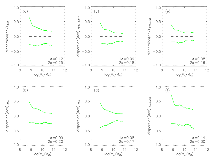
Figure 9: The scatter of the MZ relations of $0.04<z<0.12$ SFGs for the different metallicity calibrators. The green solid curves are the $95\%$ contours of metallicity dispersion in all MZ relations.

3.2 The dependence of the MZ relation

In this section, we first utilise the concentration index to investigate the morphology dependence of the MZ relation. Then, we study the morphological classifications of the MZ relation using the Sérsic index to separate galaxies into elliptical and spiral galaxies. Moreover, we explore the SFR and sSFR dependence of the MZ relation. Finally, we further investigate the dependence on the stellar population age of the MZ relation using the $D_{n}4000$ index and log(N/O).

In Figures 5(a) and 5(b), we show the MZ relations of $0.04<z\leqslant 0.06$ and $0.10<z<0.12$ SFGs with colour bars of concentration index, respectively. The colour bars show the c values per bin (0.1 dex in log($M_{\star}/M_{\sun}$) and 0.05 dex in metallicity) in the MZ relation. The green and red lines are the diagnostic lines for comparing MZ relations between the higher and lower redshift SFGs. Compared to the MZ relation of Figure 5(b), the scatter at a lower galaxy stellar mass is exhibited in Figure 5(a), showing the trend of decreasing scatter with increasing stellar mass (Tremonti et al. 2004; Zahid et al. 2012). The origin of the scatter may originate from accretion and/or mergers (Bothwell et al. 2013; Forbes et al. 2014), and Kacprazk et al. (2016) suggested that an accretion is likely to have a great influence on a galaxy’s mass.

Compared to the $0.10<z<0.12$ SFGs, the $0.04<z\leqslant 0.06$ SFGs have higher metallicities at a fixed stellar mass. At a fixed stellar mass, there is a tendency that the concentration index decreases as the metallicity increases, while at a fixed metallicity, the concentration index increases as the galaxy stellar mass increases. The index is often used to categorize galaxies into early-type and late-type with the different recommended values (Shimasaku et al. 2001; Nakamura et al. 2003; Shen et al. 2003). Hooper et al. (2007) and Ellison et al. (2008) respectively reported the dependence of the MZ relation on galaxy size, which is related to the morphology structure. Therefore the MZ relation should depend on the galaxy structure properties.

In Figures 5(c) and 5(d), the MZ relations of $0.04<z\leqslant 0.06$ and $0.10<z<0.12$ SFGs are shown using colour bars of Sérsic index, respectively. The green and red lines are the same diagnostic lines as in Figures 5(a) and 5(b). At a fixed stellar mass, there is a trend that the Sérsic index decreases with increasing metallicity, while at a fixed metallicity, the index increases with increasing stellar mass, and the change of different structural types is from disk-dominated galaxeies ($n<1.5$) to bulge-dominated galaxies ($n>2.5$, Maier et al. 2009). From Figures 5(a) and 5(b), we can see a significant trend that the concentration index almost does not change when the stellar mass and metallicity simultaneously increase. The same trend for Sérsic index also exists in Figures 5(c) and 5(d), and it also appears at the log$(M_{\star}/M_{\sun})<10.0$ in Figures 5(e) and 5(f) (with regard to the MZ relation of log$(M_{\star}/M_{\sun})>10.0$ SFGs, we will discuss it in next paragraph.), suggesting that the trend of Figures 5(e) and 5(f) is a result of some dependence of the MZ relation on SFR. In Figure 5, when a concentration index or Sersic index of the MZ relation increases, its SFR also increases. This indicates that galaxy structure properties are closely related to SFRs. In addition, we can see another significant tendency that the SFRs increase with increasing $M_{\star}$ and Z simultaneously at the log$(M_{\star}/M_{\sun})>10.0$ in Figures 5(e) and 5(f), in other word, high stellar mass galaxies with higher SFRs often have higher metallicities. This result is similar to one of Sánchez et al (2017), who studied the MZ relation with 734 CALIFA galaxies.

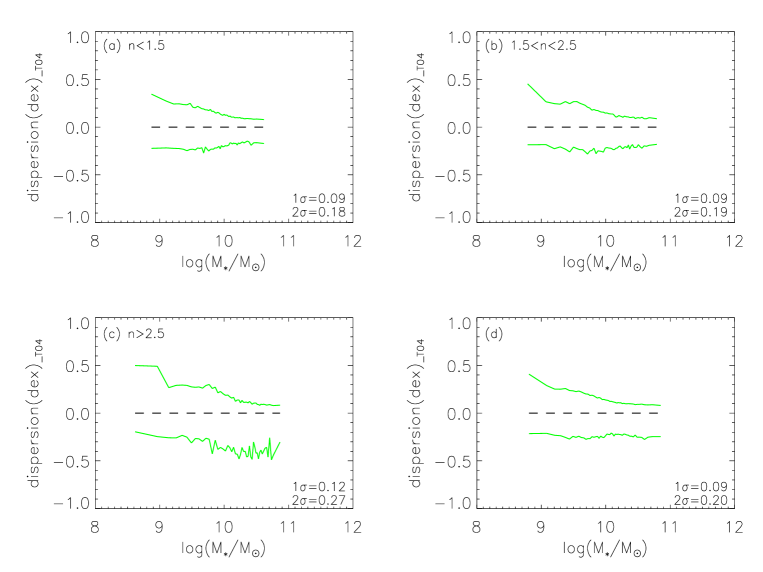
Figure 10: Comparison of the scatter of MZ relations of $0.04<z<0.12$ SFGs for the different Sérsic indexes. The symbols are the same as in Fig. 9.

In Figures 5(e) and 5(f), the log$(M_{\star}/M_{\sun})<10.0$ and log$(M_{\star}/M_{\sun})>10.0$ SFGs present a different relation between SFR and Z at a fixed stellar mass; the former population shows that the metallicity increases with decreasing SFR, whereas the latter population presents that the metallicity increases with increasing SFR. We suggest that the two group SFGs may come from differen galaxy populations, and that they are likely to possess different stellar population ages.

In Figures 5(e) and 5(f), the two galaxy populations seem to be observed in log$(M_{\star}/M_{\sun})\sim 10.0$, so we show the MZ relations using the six metallicity estimators (see the first paragraph of Section 3.3) and colour bars of sSFR in Figures 6(a) – 6(f), presenting a continuous change in sSFR in log$(M_{\star}/M_{\sun})>10.0$ SFGs. The sample shown in Figure 6 includes all SFGs with $0.04<z<0.12$. Whether do the two galaxy populations of Figure 5 exist in Figure 6, so we use the sample of 81,125 SFGs to present the MZ relation in each plot. Figure 6 displays an anticorrelation, as a whole, that galaxies with higher sSFRs have lower metallicities at a fixed stellar mass. Actually, we seem to see the two galaxy populations; one presents an anticorrelation between Z and sSFR in the lower mass galaxies, and another one exhibits a weak positive correlation between Z and sSFR in the higher mass galaxies, showing a large scatter, and this is consistent with Lara-López et al. (2013). But Salim et al. (2014) suggested that the metallicity calibrator may lead to the positive correlation between metallicity and sSFR, and that the latter galaxy population is not exist. Actually, we show the second galaxy population (see the galaxies at log(sSFR)$\lesssim-10.2$) in Figures 6(a)–6(f), showing independence on the metallicity estimator. Due to the larger stellar masses and smaller sSFRs from these figures, we suggest that these galaxies may have older stellar populations (see Figures 8(a) and 8(b)).

To show clearly the two galaxy populations, Figure 7 displays the graphs of Z versus sSFR in SFGs with different stellar mass ranges. In Figures 7(a) and 7(b), we demonstrate the relations between sSFR and 12+log(O/H) in SFGs with log$(M_{\star}/M_{\sun})<10.0$ and log$(M_{\star}/M_{\sun})>10.0$, respectively. From Figure 7(a), an anticorrelation is significant (Spearman’s coefficient, r=-0.62). In Figure 7(b), since the SFG sample with log$(M_{\star}/M_{\sun})>10.0$ are mixed with some SFGs having an anticorrelation between sSFR and 12+log(O/H), their correlation is not clear, showing their Spearman coefficient r=0.14. Figures 7(c) and 7(d) display the relations between sSFR and 12+log(O/H) in SFGs with log$(M_{\star}/M_{\sun})<10.5$ and log$(M_{\star}/M_{\sun})>10.5$, respectively. Compared to Figure 7(a), $10.0<$log$(M_{\star}/M_{\sun})<10.5$ SFGs are mixed into the SFG sample with log$(M_{\star}/M_{\sun})<10.5$ in Figure 7(c), and their correlation has weakened, showing their Spearman coefficient r=-0.47. Compared to Figure 7(b), the correlation significantly increases in Figure 7(d), showing their Spearman coefficient r=0.44. The two correlations are supported by some recent findings (Yates, Kauffmannn, & Guo 2012; Andrew & Martini 2013; Yates & Kauffmann 2014). Regarding the positive correlation at high mass galaxies, it should be investigated by more observational studies.

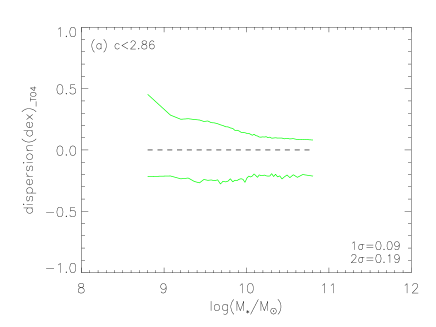
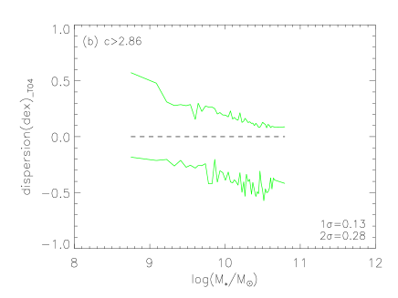
Figure 11: Comparison of the scatter of MZ relations of $0.04<z<0.12$ SFGs for the different concentration indexes. The symbols are the same as in Fig. 9.

It is well known that a $D_{n}4000$ index is a good proxy for the mean stellar ages of stellar population below $\sim 2$ Gyr. In Figures 8(a) and 8(b), we show the MZ relations of $0.04<z\leqslant 0.06$ and $0.10<z<0.12$ SFGs using the colour bars of $D_{n}4000$ index, respectively. The green and red lines are the same diagnostic lines as in Figure 5. As can be seen from Figures 8(a) and 8(b), galaxies with higher $D_{n}4000$ usually have larger Sérsic indexes at a given stellar mass (Zahid & Geller 2017).

From Figure 8(a), we can see a trend that the $D_{n}4000$ index increases when the stellar mass and metallicity increase, and this is a significant difference compared to the MZ relations with the colour bars of concentration index and Sérsic index in Figure 5, indicating that the MZ relation may be related to the stellar age of SFGs. Using a sample of Lyman-break analogure, Lian et al. (2015) found that the MZ relation is strongly correlated with $\rm D_{n}4000$, showing that galaxies having higher $D_{n}4000$ present higher metallicities at a given stellar mass. Using the similar method of Kauffmann et al. (2003b), Wu & Zhang (2013) presented a nice relation between log($M_{\star}$) and log(N/O), and suggested that the ratio may be used as a standard candle (Wu & Zhang 2013). In Figures 8(c) and 8(d), we find a clear tendency that the log(N/O) increases with increasing $M_{\star}$ and Z, implying that the MZ relation should closely link the stellar age. Actually, the tendency should be understandable. Since this $D_{n}4000$ index can provide a diagnostic of the past star formation histories of galaxies (Kauffmann et al. 2003a), we obtain the age imformation of different processes during galaxy evolution. With galaxy evolution, a huge amounts of existed or inflow gas is transformed into stars, which results in increasing galaxy stellar mass. At the same time, the evolution of massive stars and intermediate-mass stars in galaxies contributes increasing of 12+log(O/H) and log(N/O) ratio (Wu et al. 2013). As can be seen, this relationship between the stellar mass and metallcity almost accompanies the change of $D_{n}4000$ and log(N/O) ratio during the whole galaxy evolution. We confirm that the MZ relation may link closely the stellar age in SFGs (Gallazzi et al. 2005; Lian et al. 2015).

Combining with Figures 5(a), 5(b), 5(c), and 5(d), we find that the correlations between $M_{\star}$ and Z are observed at a certain range of the concentration indexes or Sérsic indexes. From Figure 5, we can see the metallicity tends to be lower in galaxies with a higher concentration index, higher Sérsic index, or higher SFR. In Figures 5(e) and 5(f), we seem to see the two galaxy populations at log$(M_{\star}/M_{\sun})\sim 10.0$, and we find that the two populations are observed by using the colour bars of sSFR in Figures 6(a) – 6(f). In addtion, Figure 7 displays the two galaxy populations, presenting clearly the two correlations between sSFR and Z, and the latter galaxy population does not depend on the metallicity estimator. We can see that the stellar mass and metallicity usually present higher in galaxies with a higher $D_{n}4000$ or higher log(N/O) ratio from Figure 8.

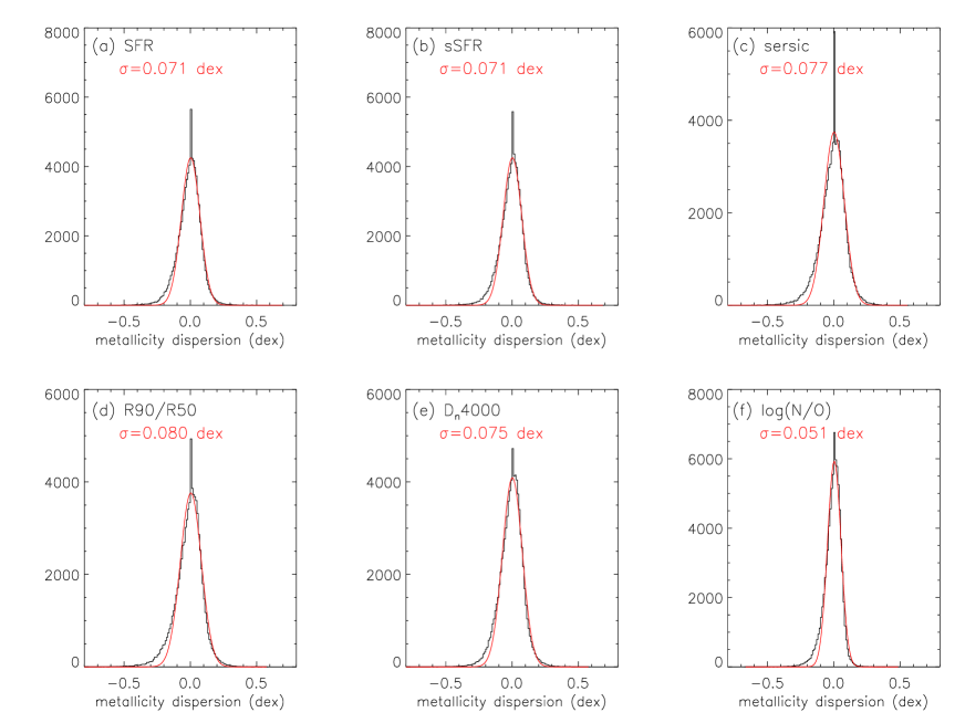
Figure 12: Comparison of metallicity dispersion in MZ-X relation, X is the third parameter (SFR, sSFR, sersic index, concentration index, $D_{n}4000$, and log(N/O), respectively.). The histogram displays the difference from the median calculated in bins of 0.05 dex in $M_{\star}$ and X. The red curve is a Gaussian with $\sigma$.

3.3 The scatter of the MZ relation

In Figure 9, we show the scatter of the MZ relation of more than $80,000$ galaxies using the six metallicity-calibrated methods, such as the metallicity diagnostics of Z94, PP04-O3N2, PP04-N2, T04, Z94, and Sander18. Firstly, the sample is classifyed into 50 almost equal galaxy bins in stellar mass, then we obtain the median value of the metallicities (get two subbins based on the median metallicity) and stellar masses, and calculate respectively the $95\%$ contours of metallicity dispersion (deviation from the median metallicity) of both subbins in each bin. The contours are shown by the green solid lines in Figure 9.

It is observed that the scatter increases with decreasing galaxy stellar mass in Figure 9 (Zahid et al. 2012). Whether the trend is real? Zahid et al. (2012) checked it using the five diagnostic calibrators of metallicities in their Figure 5, and we also examine it using another five methods of metallicity estimators in Figure 9. We find that the trend does not depend on the metallicity calibrator. Moreover, we find that the smallest scatter ($2\sigma$) is 0.16 dex in log[([N II] $\rm\lambda 6584)]/H\alpha]$ (N2) of PP04, and the largest one ($2\sigma$) is 0.30 dex in log[([N II]$\lambda 6584)$]/([O II] $\lambda 3726,3729)]$ (N2O2) of Sanders et al. (2018).

In Figures 9(a), 9(c), and 9(e), the scatter is almost symmetric for galaxies with $\sim 9.5<$ log$(M_{\star}/M_{\sun})<10.5$, while it is clearly asymmetric in Figures 9(b), 9(d), and 9(f). In Figure 4 of Zahid et al. (2012), the scatter shown is symmetric at $8.5<$log$(M_{\star}/M_{\sun})<9.5$ galaxies, and we find that the scatter symmetry may occur at the different stellar masses, determined by the different metallicity calibrator. At log$(M_{\star}/M_{\sun})>10.5$, almost all the scatter in Figures 9 begin to be asymmetric. Compared to the lower dispersion below the median values, the upper dispersion above the median values decreases significantly with the galaxy stellar mass in Figures 9(a), and 9(f), and the dispersion seems to do not decrease in Figures 9(b) and 9(d). In addition, Figures 9(a) and 9(f) show larger upper dispersion at log$(M_{\star}/M_{\sun})\sim 11.0$, showing no saturation in metallicity in the Dopita (2016) and Sanders et al. (2018) diagnostic calibrators.

In Figure 10, we display the scatter of MZ relations of SFGs with the different Sérsic indexes. Figures 10(a) and 10(b) show the scatter of MZ relations of SFGs with $n<1.5$ and $1.5<n<2.5$, respectively. Their sample sizes are 41,059 and 28,310, presenting $2\sigma=0.18$ dex and $2\sigma=0.19$ dex, respectively. Figures 10(c) and 10(d) present the scatter of MZ relations of SFGs with $n>2.5$ and the total sample, respectively. Their sample sizes are 11,564 and 80,933 (192 galaxies at $n=0$), presenting $2\sigma$ scatter of $0.27$ dex and $0.20$ dex, respectively. From Figure 10, we find that the scatter of the MZ relation colsely links the galaxy morphology, showing that elliptical galaxies have larger scatter than spiral galaxies. Certainly, the large scatter in the sample with $n>2.5$ in which the observational uncertainties in the metallicity measurement may be much higher than other two samples.

In Figure 11, the scatter of MZ relations of SFGs with the different concentration indexes is shown. Figures 11(a) and 11(b) display the scatter of MZ relations of SFGs with $c<2.86$ and $c\geqslant 2.86$, respectively. Their sample sizes are 76,286 and 4,773 (66 galaxies at c=0), presenting $2\sigma=0.19$ dex and $2\sigma=0.28$ dex, respectively. Figure 11 confirms the result of Figure 10, and the scatter of the MZ relation is closely related the galaxy morphology. In addition, we show that the scatter is composed of the superposition of several scatter of MZ relations for different type galaxies of the sample.

In addition, we utilise the scatter to compare the dependence of metallicity on galaxy properties other than mass. Figure 9(b) displays that the scatter in MZ relation is $\sigma=0.09$ dex. In Figure 12, we show metallicity dispersion in MZ - X relation, and X is the third parameter. The dispersion is calculated in bins of 0.05 dex in $M_{\star}$ and X. The dispersion reduces to $\sim 0.07$ dex when adopting this SFR paremeter in the MZ relation (see Figure 12(a)). In Figure 12(b), 12(c), 12(d), 12(e), and 12(f), the scatter decreases to $\sim 0.07$ dex, $\sim 0.08$ dex, $\sim 0.08$ dex, $\sim 0.07$ dex, and $\sim 0.05$ dex, respectively, when sSFR, Sersic index, concentration index, $D_{n}4000$, and log(N/O) are used as the third parameter. We can see a decease in scatter when adopting the third parameter in MZ relations. Compared to the scatter of $\sigma\sim 0.05$ in Mannuccci et al. (2010), the dispersion in MZ-SFR relation is $\sigma\sim 0.07$, and this difference may be related to the different SFG sample. In addtion, we find that the dispersion in MZ-log(N/O) relation is $\sigma\sim 0.05$, showing the smallest dispersion among these galaxy properties, and this may originate from that the log(N/O) ratio is used to calculate the SFG metallicity.

4 Summary

Utilising the observational data of 86,111 SFGs obtained from the catalogue of the SDSS DR7 MPA-JHU emission-line measurements, we investigate the MZ relation evolution. Also, using the concentration index, Sérsic index, selected both from the NYU-VAGC data, log(N/O), SFR, sSFR, and $D_{n}4000$, we explore the dependence and scatter of the MZ relations of $0.04<z\leqslant 0.06$ and $0.10<z<0.12$ SFGs. Our main results are summarized as followings:

1. Under the $\rm log(L_{H\alpha})>41.0$ threshold, the $0.04<z\leqslant 0.06$ ($0.10<z<0.12$) SFGs with $9.2<\rm log(M_{\star}/M_{\sun})<9.5$ have higher (lower) $\sim 0.1$ dex in metallicity than their corresponding control sample, and the K-S test shows that the two samples (both median(log(SFR))$>0.0$) present the MZ relation evolution.

2. Under the $\rm log(L_{[\rm O~{}\sc{III}]})>39.7$ threshold, the $0.04<z\leqslant 0.06$ SFGs with $9.2<\rm log(M_{\star}/M_{\sun})<9.5$ have almost no difference in metallicity compared to their corresponding control sample, and the K-S test ($p_{null}=51\%$, see Table 1) shows that the MZ relation evolution is not found in the two samples (both median(log(SFR))$<0.0$). However, the $0.10<z<0.12$ SFGs with $9.2<\rm log(M_{\star}/M_{\sun})<9.5$ have the same result as the $\rm log(L_{H\alpha})>41.0$ threshold mentioned above ($p_{null}=1.42\times 10^{-3}\%$, see Table 1), compared to their corresponding control sample (both median(log(SFR))$>0.0$). These show that the evolution of the MZ relation is clearly observed in the higher SFR SFGs (e.g. median(log(SFR))$>0.0$)), and that almost no evolution of the MZ relation is found in the SFGs at lower SFRs (e.g. median(log(SFR))$<0.0$). We suggest that these originate from the speciality of the sample.

3. Under the same stellar mass and Sérsic index (concentration index), we show that the $0.04<z\leqslant 0.06$ SFGs have always higher $\sim 0.1-0.2$ dex in metallicity than the $0.10<z<0.12$ SFGs. This shows that the MZ relation evolution exists and does not depend on the elliptical or spiral galaxies.

4. Utilising the concentration index and Sérsic index, SFR, we find that the metallicity tends to be lower in galaxies with a higher concentration, higher Sérsic index, or higher SFR. In addition, we can see that the stellar mass and metallicity usually present higher in galaxies with a higher $D_{n}4000$ or higher log(N/O) ratio.

5. With regard to a possibility of the two galaxy populations in the MZ relation at log$(M_{\star}/M_{\sun})\sim 10.0$, we find that they may exist by using color bars of sSFR in Figures 6(a) – 6(f). In addition, we present clearly an anticorrelation and a positive correlation between sSFR and 12+log(O/H) at log$(M_{\star}/M_{\sun})\sim 10.0$ and 10.5, respectively. From the dependence on the $D_{n}4000$ index and log(N/O) in the MZ relation, we confirm that the MZ relation may link closely the stellar age in SFGs.

6. The scatter of the MZ relation increases with decreasing stellar mass, and we show that the trend does not depend on the metallicity calibrator. Also, we find that the scatter symmetry may occur at different stellar masses, determined by the different metallicity calibrator. Moreover, almost all the scatter of the MZ relations begin to be asymmetric at log$(M_{\star}/M_{\sun})>10.5$.

7. We find that the scatter of the MZ relation colsely links the galaxy morphology, presenting that the elliptical galaxies often have larger scatter than the spiral galaxies. This may be originated from the large scatter in the SFG sample with $n>2.5$ or $c>2.86$. In addition, we show that the scatter is composed of the superposition of several scatter of the MZ relation for different type galaxies.

8. We show that metallicity dispersion in MZ - X relation, and X is SFR, sSFR, Sérsic index, concentration index, $D_{n}4000$, and log(N/O), respectively. We confirm that the MZ relation depends on the six galaxy properties.

References

- Abazajian (2009) Abazajian, K. N., Adelman-McCarthy, J. K., Agüeros, M. A. et al. 2009, ApJS, 182, 543
- Andrews (2013) Andrews, B. H., & Martini, P. 2013, ApJ, 765, 140
- Baldwin (1981) Baldwin, J. A., Phillips, M. M., & Terlevich, R. 1981, PASP, 93, 5
- Balogh et al (1999) Balogh, M. L., Morris, S. L., Yee, H. K. C., Carlberg, R. G., & Ellingson, E. 1999, ApJ, 527, 54
- Barrera-Ballesteros (2017) Barrera-Ballesteros, J. K., Sánchez, S. F., Heckman, T., et al. 2017, ApJ, 844, 80
- Belli (2013) Belli, S., Jones, T., Ellis, R. S., & Richard, J. 2013, ApJ, 772, 141
- Blanton (2005) Blanton, M. R. et al., 2005, AJ, 129, 2562
- Bothwell (2013) Bothwell, M. S., Maiolino, R., Kennicutt, R., et al. 2013, MNRAS, 433, 1425
- Brown et al. 2017 (2017) Brown, T., Cortese, L., Catinella, B., & Kilborn, V. 2018, MNRAS, 473, 1868
- Chabrier 2003 (2003) Chabrier, G. 2003, PASP, 115, 763
- Christensen 2012 (2012) Christensen, L., Richard, J., Hjorth, J., et al. 2012, MNRAS, 427, 1953
- Cullen et al. 2014 (2014) Cullen, C., Cirasuolo, M., McLure, R. J., Dunlop, J. S., & Bowler, R. A. A. 2014, MNRAS, 440, 2300
- Dopita 2016 (2016) Dopita, M, A. 2016, APSS, 361, 61
- Ellison et al. 2008 (2008) Ellison, S. L., Patton, D. R., Simard, L., & McConnachie, A. W. 2008, ApJL, 672, 107
- Erb et al. 2006 (2006) Erb, D. K., Shapley, A. E., Pettini, M., et al. 2006, ApJ, 644, 813
- Forbes et al. 2014 (2014) Forbes, J. C., Krumholz, M. R., Burkert, A., & Dekel, A. 2014, MNRAS, 443, 168
- Gallazzi et al. 2005 (2005) Gallazzi, A., Stéphane, C., Brinchmann, J., et al. 2005, MNRAS, 362, 41
- Guo et al. 2016 (2016) Guo,Y.C., et al. 2016, ApJ, 822, 103
- Henry et al. 2013 (2013) Henry, A., Scarlata, C., Domínguez, A., Malkan, M., Martin, C. L., et al. 2013, ApJL, 776, 27
- Hoopes 2007 (2007) Hoopes, C. G., Heckman, T. M., Salim, S., et al. 2007, ApJS, 173, 441
- Hunt 2016 (2016) Hunt, L., Dayal, P., Magrini, L., & Ferrara, A. 2016, MNRAS, 463, 2002
- Juneau 2014 (2014) Juneau S. et al., 2014, ApJ, 788, 88
- Kacprzak et al. 2016 (2016) Kacprzak, G. G., van de Voort, F., Glazebrook, K., et al. 2016, ApJL, 826, L11
- Kashino et al. 2017 (2017) Kashino, D., Silverman, J. D., Sanders, D., et al. 2017, ApJ, 835, 88
- Kauffmann et al. 2003 (2003) Kauffmann, G., Heckman, T. M., Tremonti, C., et al. 2003a, MNRAS, 346, 1055
- Kauffmann et al. 2003 (2003) Kauffmann, G., Heckman, T. M., White, S. D. M., et al. 2003b, MNRAS, 341, 54
- Kewley & Dopita 2002 (2002) Kewley, L. J., & Dopita, M. A. 2002, ApJS, 142, 35
- Kewley & Ellison 2008 (2008) Kewley, L. J., & Ellison, S. L. 2008, ApJ, 681, 1183
- Kewley et al. 2006 (2006) Kewley, L. J., Grovers, B., Kauffmann, G., & Heckman, T. 2006, MNRAS, 372, 961
- Kewley et al. 2005 (2005) Kewley, L. J., Jansen, R. A., & Geller, M. J. 2005, PASP, 117, 227
- Kroupa 2001 (2001) Kroupa, P. 2001, MNRAS, 322, 231
- Lara-López et al. 2010 (2010) Lara-López, M. A., Bongiovanni, A., et al. 2010, A&A, 519, 31
- Lara-López et al. 2013 (2013) Lara-López, M. A., Hopkins, A. M., López-Sánchez, A. R., et al. 2013, MNRAS, 434, 451
- Lequeux et al. 1979 (1979) Lequeux, J., Peimbert,M., Rayo, J. F., Serrano, A., & Torres-Peimbert, S. 1979, A&A, 80, 155
- Lian et al. 2015 (2015) Lian, J. H., Li, J. R., Yan, W., & Kong, X. 2015, MNRAS, 446, 1449
- Maier et al. 2009 (2009) Maier, C., Lilly, S. J., Zamorani, G., et al. 2009, ApJ, 694, 1099
- Maier et al. 2014 (2014) Maier, C., Lilly, S. J., Ziegler, B. L., et al. 2014, ApJ, 792, 3
- Maiolino et al. 2008 (2008) Maiolino, R., Nagao, T., Grazian, A., et al. 2008, A&A, 488, 463
- Mannucci et al. 2010 (2010) Mannucci, F., Cresci, G., Maiolino, R., Marconi, A., & Gnerucci, A. 2010, MNRAS, 408, 2115
- Nakamura et al. 2003 (2003) Nakamura, O., Fukugita, M., Yasuda, N., et al. 2003, AJ, 125, 1682
- Peng et al. 2015 (2015) Peng, Y., Maiolino, R., & Cochrane, R. 2015, Nature, 521, 192
- Pettini & Pagel. 2004 (2004) Pettini, M., & Pagel,B. E. J. 2004, MNRAS, 348, 59
- Pilyugin et al. 2006 (2006) Pilyugin, L. S., Thuan, T. X., & Vílchez, J. M. 2006, MNRAS, 367, 1139
- Pilyugin et al. 2010 (2010) Pilyugin, L. S., Vílchez, J. M., Cedrés, B., & Thuan, T. X. 2010, MNRAS, 403, 896
- Salim et al. 2015 (2015) Salim, S., Lee, J. C., Davé, R., & Dickinson, M. 2015, ApJ, 808, 25
- Salim et al. 2014 (2014) Salim, S., Lee, J. C., Ly, C., et al. 2014, ApJ, 797, 126
- Sánchez et al. 2013 (2013) Sánchez, S. F., Rosales-Ortega, F. F., Jungwiert, B., et al. 2013, A&A, 554, 58
- Sánchez et al. 2017 (2017) Sánchez, S. F., Barrera-Ballesteros, J. K., Sánchez-Menguiano, L., et al. 2017, MNRAS, 469, 2121
- Sanders et al. 2015 (2015) Sanders, R. L., Shapley, A. E., Kriek, M., et al. 2015, ApJ, 799, 138
- Sanders et al. 2018 (2018) Sanders, R. L., Shapley, A. E; Mariska, K., et al. 2018, ApJ, 858, 99
- Shen et al. 2003 (2003) Shen, S., Mo, H. J., White, S. D. M., et al. 2003, /mnras, 343, 978
- Shimasaku et al. 2001 (2001) Shimasaku, K., Fukugita, M., Doi, M., et al. 2001, AJ, 122, 1238
- Stott et al. 2013 (2013) Stott, J. P., Sobral, D., Bower, R., et al. 2013, MNRAS, 436, 1130
- Tremonti et al. 2004 (2004) Tremonti, C. A., Heckman, T. M., Kauffmann, G., et al. 2004, ApJ, 613, 898
- Troncoso et al. 2014 (2014) Troncoso, P., Maiolino, R., Sommariva, V. et al. 2014, A&A, 563, 58
- Wu et al. 2013 (2013) Wu, Y.-Z., & Zhang, S.-N. 2013, MNRAS, 436, 934
- Wu et al. 2016 (2016) Wu, Y.-Z., Zhang, S.-N., Zhao, Y.-H., & Zhang, W. 2016, MNRAS, 457, 2929
- Wuyts et al. 2014 (2014) Wuyts, E., Kurk, J., Forster Schreiber, N. M., et al. 2014, ApJ, 789, 40
- Wuyts et al. 2012 (2012) Wuyts, E., Rigby, J. R., Sharon, K., & Gladders, M. D. 2012, ApJ, 755, 73
- Wuyts et al. 2016 (2016) Wuyts, E., Wisnioski, E., Fossati, M., et al. 2016, ApJ, 827, 74
- Yabe et al. 2015 (2015) Yabe, K., Ohta, K., Akiyama, M., et al. 2015, PASJ, 67, 102
- Yabe et al. 2014 (2014) Yabe, K., Ohta, K., Iwamuro, F., et al. 2014, MNRAS, 437, 3647
- Yates et al. 2012 (2012) Yates, R. M., Kauffmann, G., & Guo, Q. 2012, MNRAS, 422, 215
- Yates et al. 2014 (2014) Yates, R. M., & Kauffmann, G. 2014, MNRAS, 439, 3834
- Zahid et al. 2012 (2012) Zahid, H. J., Bresolin, F., Kewley ,L. J., Coil, A. L., & Davé, R. 2012, ApJ, 750, 120
- Zahid et al. 2015 (2015) Zahid, H. J., Damjanov, I., Geller, M. J., & Chilingarian, I. 2015, ApJ, 806, 122
- Zahid & Geller 2017 (2017) Zahid, H. J & Geller, M. J. 2017, ApJ, 841, 32
- Zahid et al. 2013 (2013) Zahid, H. J., Geller, M. J., Kewley, L. J., et al. 2013, ApJL, 771, 19
- Zahid et al. 2014 (2014) Zahid, H. J., Kashino, D., Silverman, J. D., et al. 2014, ApJ, 792, 75
- Zaritsky et al. 1994 (1994) Zaritsky, D., Kennicutt, R. C., & Huchra, J. P. 1994, ApJ, 420, 87
- Zhang et al. 2008 (2008) Zhang, W., Kong, X., & Cheng, F. Z. 2008, CHJAA, 8, 211