A discrete least squares collocation method for two-dimensional nonlinear time-dependent partial differential equations

Abstract

In this paper, we develop regularized discrete least squares collocation and finite volume methods for solving two-dimensional nonlinear time-dependent partial differential equations on irregular domains. The solution is approximated using tensor product cubic spline basis functions defined on a background rectangular (interpolation) mesh, which leads to high spatial accuracy and straightforward implementation, and establishes a solid base for extending the computational framework to three-dimensional problems. A semi-implicit time-stepping method is employed to transform the nonlinear partial differential equation into a linear boundary value problem. A key finding of our study is that the newly proposed mesh-free finite volume method based on circular control volumes reduces to the collocation method as the radius limits to zero. Both methods produce a large constrained least-squares problem that must be solved at each time step in the advancement of the solution. We have found that regularization yields a relatively well-conditioned system that can be solved accurately using QR factorization. An extensive numerical investigation is performed to illustrate the effectiveness of the present methods, including the application of the new method to a coupled system of time-fractional partial differential equations having different fractional indices in different (irregularly shaped) regions of the solution domain.

1 Introduction

Meshfree and meshless methods have been applied widely to solve partial differential equations (PDEs) on irregular domains due to their flexibility in dealing with a wide variety of geometries, see, for example, [1, 2, 3]. In this work, we take an alternative approach to deal with irregular domains and develop efficient regularized discrete least squares (LS) collocation and finite volume methods (FVMs) for solving nonlinear time-dependent partial differential equations in irregular two-dimensional domains.

Our work is motivated by the need to resolve multiscale transport processes in heterogeneous porous media using upscaling methods. As an example, the Extended Distributed Microstructure Model proposed in [4] approximates the macroscopic flux as the average of the microscopic fluxes computed over micro-cells having geometrical features representative of the actual porous micro-structure. Such an approach avoids the need for any effective parameters in the formulation and accounts more accurately for a non-equilibrium field evolution within the micro-cells. It is therefore important to have fast and flexible computational methods for computing over complex, irregularly shaped domains (micro-cells) that are often established directly from images of the porous microstructure. Recent work highlights that memory effects and non-Fickian behaviour are important physical mechanisms evident for lignocellulosic materials such as wood [5]. The contribution of our work is to investigate new time-fractional models for use in our microscale formulation that can address these issues for regions of differing fractional properties within the micro-cell.

LS Galerkin and collocation methods have been widely applied to solve PDEs due to their computational advantages and simplifications, see for example [6, 7, 8, 9, 10, 11, 12]. In the mesh-based (LS) Galerkin method for solving FDEs on irregular domains, the domain is approximately divided into subdomains, on which basis functions are defined. The division of the irregular domain may cause errors that affect the accuracy of the method. If moving boundary conditions are considered in this method, the irregular domain must be redivided and the mass and stiffness matrices recomputed. These are costly operations.

The LS collocation (LSC) method with a completely orthogonal computational mesh has been used to solve PDEs on irregular domains. Its advantages include simple implementation and high accuracy; see [6, 8, 13, 14, 15, 16] for further details. However, these methods may yield an ill-conditioned LS system, which may cause computational difficulties in real applications. In this work, this disadvantage is overcome by using a generalized regularization technique [17, 18], which stabilizes the solution procedure while preserving high accuracy.

The idea of developing the LSC method for solving time-dependent PDEs has not been fully explored in previous work (see, for example, [8]). The main contribution of our work is to combine this idea with the linearized time-stepping method to develop regularized (penalized) LS methods for solving nonlinear time-dependent PDEs on irregular domains, yielding linear systems that can be solved efficiently.

We first develop the regularized LSC method and least squares finite volume method (LSFVM) for solving a two-dimensional linear boundary-value problem on an irregular domain $\Omega$ (see (1)). The key idea of the present LS method is to approximate the solution by the tensor product of cubic spline basis functions defined on a rectangular mesh, for a division of a suitable rectangular domain $\Omega_{\Box}\supset\Omega$, leading to high spatial accuracy, straightforward implementation, and easy extension to a three-dimensional framework. The use of regularization makes the penalized LS system relatively well-conditioned with the smallest singular value of order $O(\sqrt{\delta})$, where $\delta>0$ is the regularization parameter that balances accuracy and well-conditioning of the LS system. We use QR decomposition to solve the LS problem accurately and stably. Numerical simulations show that a regularization parameter $\delta=0.01$ yields satisfactory numerical solutions.

We then extend our LSC/LSFVM to solve a nonlinear time-dependent PDE. Our approach is to apply a semi-implicit time-stepping method (see [20]) to transform the nonlinear time-dependent PDE into a linear boundary value problem, which is solved by the penalized LSC method or LSFVM developed for the model problem. One advantage of the present LS method is that it requires solution of linear LS systems. We present numerical simulations to verify the effectiveness of the present LS method, including a fractional model with two fractional indices that models diffusion in a composite medium.

A finite element method based on weighted extended B-splines on a regular grid as basis functions was proposed to solve Dirichlet problems on irregular domains in [21], yielding a well-conditioned linear system. Recently, a least squares radial basis function partition-of-unity method has been developed in [11], which can deal with irregular domains easily. The newly developed meshfree LSFVM in [19] is another alternative to deal with irregular domains and achieves high accuracy in solving multi-phase porous media models. A key finding of the work presented here is that as the radius of the circular finite volumes approaches zero, the LSC method is recovered.

This paper is organized as follows. Section 2 presents the penalized LSC method and LSFVM for a two-dimensional linear model problem. We also investigate the conditioning of the LS system and seek techniques for solving it efficiently. In Section 3, we show how to extend the LS method for the linear model problem to nonlinear time-dependent PDEs. Two numerical examples are given in Section 4 to show the effectiveness of the LSC method for solving nonlinear generalized PDEs and a coupled system of time-fractional PDEs. We make some closing remarks in Section 5.

2 Discrete least squares for a model problem

We develop the regularized LSC method and LSFVM for the following model problem

$$u(x,y)-\nu\Delta u(x,y)=f(x,y),{\quad}(x,y)\in\Omega,$$ (1)

subject to the following generalized boundary condition

$$\mathcal{B}(u)=u_{b}\quad\text{on}\quad\partial\Omega,$$ (2)

where $\Delta$ is the Laplacian in two-dimensional space; $\nu$ is a positive scalar parameter; $\mathcal{B}$ represents Dirichlet, Neumann, or mixed boundary conditions; and $\Omega$ is an irregular domain with a piecewise smooth boundary; Figure 1 shows several irregular domains that will be used for the numerical computations performed in this work to verify our discretisation methods.

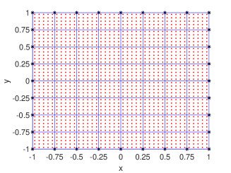
(a)

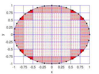
(b)

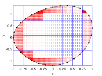
(c)

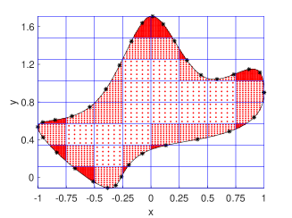
(d)

Figure 1: The division of the different domains (the area surrounded by the black curve for (b), (c), and (d)) with the corresponding boundary points (stars $*$) and collocation points (red dots $\bullet$).

2.1 Notation

A background (interpolation) mesh and a corresponding set of basis functions are needed for the LS method. For any finite domain $\Omega$, we can find a suitable rectangular domain $\Omega_{\Box}$ such that $\Omega\subset\Omega_{\Box}=(a,b)\times(c,d)$; see Figure 1. The default values of $a,b,c,$ and $d$ are given by $a=\inf\{x|(x,y)\in\Omega\}$, $b=\sup\{x|(x,y)\in\Omega\}$, $c=\inf\{y|(x,y)\in\Omega\}$, and $d=\sup\{y|(x,y)\in\Omega\}$, respectively.

Let $\delta_{x}=\{x_{i}\}$ (or $\delta_{y}=\{y_{j}\}$) be a division of $I^{x}$ (or $I^{y}$), satisfying $a=x_{0}<x_{1}<\cdots<x_{N_{x}}=b$ (or $c=y_{0}<y_{1}<\cdots<y_{N_{y}}=d$). Denote $I_{i,j}={I}^{x}_{i}\times{I}^{y}_{j}$, where $I^{x}_{i}=(x_{i-1},x_{i})$ and $I^{y}_{j}=(y_{j-1},y_{j})$. Then the domain ${\Omega}_{\Box}$ is divided into non-overlapping rectangular subdomains that satisfy ${\bar{\Omega}_{\Box}}=\cup_{i,j}\bar{I}_{i,j}$.

The $C^{1}$ continuous basis function space defined on the mesh $\delta_{x}\times\delta_{y}$ is given by

$$\mathcal{M}_{\Omega}(\delta_{x}\times\delta_{y})=\left\{v\,:\,v\in C^{1}(\bar{\Omega}),\;v|_{\bar{I}_{i,j}}\in P_{3}(\bar{I}^{x}_{i})\otimes P_{3}(\bar{I}^{y}_{j}),\;I_{i,j}\cap\Omega\neq\emptyset\right\},$$ (3)

where $P_{k}(\bar{I})$ denotes the polynomial space defined on the interval $\bar{I}$ with degree no greater than $k$. In this work, we apply the tensor product cubic spline basis functions defined on the mesh grids $\delta_{x}\times\delta_{y}$ to approximate the solution of the differential equation. Therefore, any function $v\in\mathcal{M}_{\Omega}(\delta_{x}\times\delta_{y})$ can be expressed by $v|_{\bar{I}_{i,j}}=\sum_{m=1}^{4}\sum_{n=1}^{4}c^{(i,j)}_{m,n}\phi^{(i)}_{m}(x)\psi^{(j)}_{n}(y)$, where the cubic spline basis functions $\phi^{(i)}_{m}(x)$ in the $x$ direction are given by (see [22]):

$$\phi^{(i)}_{1}(x) =2\hat{x}^{3}-3\hat{x}^{2}+1,{\qquad}\phi^{(i)}_{2}(x)=(x_{i}-x_{i-1})(\hat{x}^{3}-2\hat{x}^{2}+\hat{x}),$$ (4)

$$\phi^{(i)}_{3}(x) =-2\hat{x}^{3}+3\hat{x}^{2},{\qquad\quad}\phi^{(i)}_{4}(x)=(x_{i}-x_{i-1})(\hat{x}^{3}-\hat{x}^{2}),$$

$$\hat{x} =(x-x_{i-1})/(x_{i}-x_{i-1}).$$

The basis functions $\psi^{(j)}_{n}(y)(1\leq n\leq 4)$ in the $y$ direction are defined similarly.

Before presenting the LS method, we introduce further notation. Let

$$\{\Phi_{1}(x,y),\Phi_{2}(x,y),\dotsc,\Phi_{M}(x,y)\}$$

be a basis for $\mathcal{M}_{\Omega}(\delta_{x}\times\delta_{y})$. Denote

$$\Phi(x,y) =(\Phi_{1}(x,y),\Phi_{2}(x,y),\dotsc,\Phi_{M}(x,y))^{T},$$ (5)

$$\Delta\Phi(x,y) =(\Delta\Phi_{1}(x,y),\Delta\Phi_{2}(x,y),\dotsc,\Delta\Phi_{M}(x,y))^{T},$$ (6)

with $\Phi^{T}(x,y)=(\Phi(x,y))^{T}$ and $\Delta\Phi^{T}(x,y)=(\Delta\Phi(x,y))^{T}$. For any $\mathbf{c},\mathbf{c}^{n}\in\mathbb{R}^{M}$, denote $\mathbf{c}=(c_{1},c_{2},\dotsc,c_{M})^{T}$ and $\mathbf{c}^{n}=(c_{1}^{n},c_{2}^{n},\dotsc,c_{M}^{n})^{T}$. Then any $U_{h}\in\mathcal{M}_{\Omega}(\delta_{x}\times\delta_{y})$ can be expressed by

$$U_{h}(x,y)=\Phi^{T}(x,y)\mathbf{c}=(\Phi^{T}\mathbf{c})(x,y),{\quad}\mathbf{c}\in\mathbb{R}^{M}.$$ (7)

The set $\mathcal{S}^{(p,q)}_{\Omega}$ of collocation points in the domain $\Omega$ is defined by the following four steps.

• Step 1) Let $p$ and $q$ be two positive integers. Define $\widehat{\mathcal{S}}_{p,q}$ as

  $$\widehat{\mathcal{S}}_{p,q}=\left\{(\hat{x}_{k},\hat{y}_{\ell})\,:\,1\leq k\leq p,\;1\leq\ell\leq q\right\},$$

  where $(\hat{x}_{k},\hat{y}_{\ell})=(\frac{2k-1}{2p},\frac{2\ell-1}{2q})$. Obviously, $\widehat{\mathcal{S}}_{p,q}$ is a set of points uniformly distributed in the reference domain $(0,1)\times(0,1)$.

• Step 2) For any $1\leq i\leq N_{x}$ and $1\leq j\leq N_{j}$, define the mapping $\mathcal{P}_{i,j}$ as follows:

  $$\mathcal{P}_{i,j}(\widehat{\mathcal{S}}_{p,q})=\{(\widetilde{x}_{k},\widetilde{y}_{\ell})\,:\,\widetilde{x}_{k}={h_{i}^{x}\hat{x}_{k}}+x_{i-1},\;\widetilde{y_{\ell}}={h_{j}^{y}\hat{y}_{\ell}}+y_{j-1},\;(\hat{x}_{k},\hat{y}_{\ell})\in\widehat{\mathcal{S}}_{p,q}\},$$ (8)

  where $h_{i}^{x}=x_{i}-x_{i-1}$ and $h_{j}^{y}=y_{j}-y_{j-1}$.

• Step 3) Define ${\mathcal{S}}^{(i,j)}_{p,q}$ as follows:

  $${\mathcal{S}}^{(i,j)}_{p,q}=\left\{\begin{aligned} &\mathcal{P}_{i,j}(\widehat{\mathcal{S}}_{5,5}),&&{\quad}I_{i,j}\subset\Omega,\\ &\mathcal{P}_{i,j}(\widehat{\mathcal{S}}_{p,q}),&&{\quad}\text{two or three vertices of the rectangle }I_{i,j}\text{ are in }\Omega,\\ &\mathcal{P}_{i,j}(\widehat{\mathcal{S}}_{2p,2q}),&&{\quad}\text{only one vertex of the rectangle }I_{i,j}\text{ is in }\Omega,\\ &\emptyset,&&{\quad}\text{otherwise}.\end{aligned}\right.$$ (9)

  The set ${\mathcal{S}}^{(i,j)}_{10,10}$ is applied if we do not specify $p$ and $q$.

• Step 4) The set $\mathcal{S}^{(p,q)}_{\Omega}$ of collocation points is given by

  $$\mathcal{S}^{(p,q)}_{\Omega}=\Big{(}\bigcup_{i,j}{\mathcal{S}}^{(i,j)}_{p,q}\Big{)}\bigcap\Omega.$$ (10)

The set $\mathcal{S}^{(p,q)}_{\Omega}$ has more collocation points in the cells $I_{i,j}$ near the boundary of $\Omega$, which makes the coefficient matrix from the LS method more well-conditioned than the matrix based on the uniform distribution of collocation point set $\mathcal{\overline{S}}^{(p,q)}_{\Omega}$ defined by

$$\mathcal{\overline{S}}^{(p,q)}_{\Omega}=\Big{(}\bigcup_{i,j}\mathcal{P}_{i,j}(\widehat{\mathcal{S}}_{p,q})\Big{)}\bigcap\Omega.$$ (11)

For simplicity, we denote $\xi^{(in)}_{i}=(x^{(in)}_{i},y^{(in)}_{i})\in\mathcal{S}^{(p,q)}_{\Omega}$, $1\leq i\leq N_{in}$ . The set of collocation points on $\partial\Omega$ is denoted by $\mathcal{S}^{(p,q)}_{\partial\Omega}$ with $\xi^{(b)}_{i}=(x^{(b)}_{i},y^{(b)}_{i})\in\mathcal{S}^{(p,q)}_{\partial\Omega}$, $1\leq i\leq N_{b}$. Figure 1 shows the distribution of collocation and boundary points in different domains. Figure 2 contrasts $\mathcal{\overline{S}}^{(p,q)}_{\Omega}$ and $\mathcal{S}^{(p,q)}_{\Omega}$ for $p=q=8$.

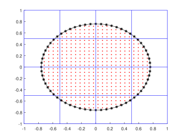
(a) Distribution of $\mathcal{\overline{S}}^{(8,8)}_{\Omega}$.

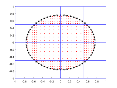
(b) Distribution of $\mathcal{S}^{(8,8)}_{\Omega}$.

Figure 2: Distribution of collocation points of $\mathcal{\overline{S}}^{(8,8)}_{\Omega}$ and $\mathcal{S}^{(8,8)}_{\Omega}$, where $\Omega=\{(x,y)|x^{2}+y^{2}\leq 0.76^{2}\}$, $\Omega_{\Box}=(-1,1)^{2}$, and $N_{x}=N_{y}=4$.

2.2 LSC method and LSFVM

We now present the penalized LSC method and LSFVM for solving the model problem (1), yielding a better-conditioned linear system that can be solved by many known methods.

2.2.1 LSC method

Replacing $u(x,y)$ in (1) with $U_{h}(x,y)=\Phi^{T}(x,y)\mathbf{d}$ defined by (7), and letting $(x,y)=\xi^{(in)}_{i}\in\mathcal{S}^{(p,q)}_{\Omega}$, we obtain

$$\left(\Phi^{T}(\xi^{(in)}_{i})-\nu\Delta\Phi^{T}(\xi^{(in)}_{i})\right)\mathbf{d}=f(\xi^{(in)}_{i}),{\quad}1\leq i\leq N_{in},$$ (12)

subject to boundary conditions

$$\mathcal{B}(U_{h}(\xi^{(b)}_{i}))=\mathcal{B}(\Phi^{T}(\xi^{(in)}_{i}))\mathbf{d}=u_{b}(\xi^{(b)}_{i}),{\quad}1\leq i\leq N_{b}.$$ (13)

Clearly, the system (12)-(13) is overdetermined. If we enforce boundary conditions exactly and other conditions in a LS sense, we obtain the following constrained LS problem

$$\mathbf{c} =\arg\min_{\mathbf{d}\in\mathbb{R}^{M}}\,\sum_{i=1}^{N_{in}}\left((\Phi^{T}(\xi^{(in)}_{i})-\nu\Delta\Phi^{T}(\xi^{(in)}_{i}))\mathbf{d}-f(\xi^{(in)}_{i})\right)^{2}$$ (14)

$$=\arg\min_{\mathbf{d}\in\mathbb{R}^{M}}\,\|(\mathbf{A}_{in}-\nu\mathbf{S}_{in})\mathbf{d}-\mathbf{f}_{in}\|^{2},$$

$$\mbox{subject to}{\quad}\mathbf{A}_{b}\mathbf{d}=\mathbf{u}_{b}=\left(u_{b}(\xi^{(b)}_{1}),u_{b}(\xi^{(b)}_{2}),\dotsc,u_{b}(\xi^{(b)}_{N_{b}})\right)^{T},$$

where $\mathbf{f}_{in}=(f(\xi^{(in)}_{1}),f(\xi^{(in)}_{2}),\dotsc,f(\xi^{(in)}_{N_{in}}))^{T}$, and the matrices $\mathbf{A}_{in},\mathbf{S}_{in}\in R^{N_{in}\times M}$ and $\mathbf{A}_{b}\in R^{N_{b}\times M}$ are given by

$$\mathbf{A}_{in}=\left[\begin{array}[]{cccc}\Phi^{T}(\xi^{(in)}_{1})\\ \Phi^{T}(\xi^{(in)}_{2})\\ \vdots\\ \Phi^{T}(\xi^{(in)}_{N_{in}})\\ \end{array}\right],{\quad}\mathbf{S}_{in}=\left[\begin{array}[]{cccc}\Delta\Phi^{T}(\xi^{(in)}_{1})\\ \Delta\Phi^{T}(\xi^{(in)}_{2})\\ \vdots\\ \Delta\Phi^{T}(\xi^{(in)}_{N_{in}})\\ \end{array}\right],{\quad}\mathbf{A}_{b}=\left[\begin{array}[]{cccc}\mathcal{B}(\Phi^{T}(\xi^{(b)}_{1}))\\ \mathcal{B}(\Phi^{T}(\xi^{(b)}_{2}))\\ \vdots\\ \mathcal{B}(\Phi^{T}(\xi^{(b)}_{N_{b}}))\\ \end{array}\right].$$ (15)

One way to enforce boundary conditions approximately is to include them directly in the overdetermined system using a weight $\lambda$ that can be varied according to how accurately we want the conditions to be satisfied (see [23]). This quadratic-penalty approach yields the following unconstrained LS formulation:

$$\mathbf{c}_{\lambda} =\arg\min_{\mathbf{d}\in\mathbb{R}^{M}}\left\{\|(\mathbf{A}_{in}-\nu\mathbf{S}_{in})\mathbf{d}-\mathbf{f}_{in}\|^{2}+\lambda^{2}\|\mathbf{A}_{b}\mathbf{d}-\mathbf{u}_{b}\|^{2}\right\}$$ (16)

$$=\arg\min_{\mathbf{d}\in\mathbb{R}^{M}}\left\|\left(\begin{array}[]{c}\mathbf{A}_{in}-\nu\mathbf{S}_{in}\\ \lambda\mathbf{A}_{b}\\ \end{array}\right)\mathbf{d}-\left(\begin{array}[]{c}\mathbf{f}_{in}\\ \lambda\mathbf{u}_{b}\\ \end{array}\right)\right\|^{2}.$$

Large values of $\lambda$ increase the importance of satisfying the boundary residuals relative to the interior residuals, that is, the boundary conditions will be more accurately satisfied as $\lambda$ becomes larger; see [8, 23].

There is computational difficulty in solving both (14) and (16) due to the ill-conditioning (even rank deficiency) of the matrices $\mathbf{A}_{in}-\nu\mathbf{S}_{in}$ and $\binom{\mathbf{A}_{in}-\nu\mathbf{S}_{in}}{\lambda\mathbf{A}_{b}}$. This is caused by a possibly very small support of some cells $I_{i,j}$ in $\Omega$, which means that $|I_{i,j}\cap\Omega|/|I_{i,j}|$ is too small to contain enough collocation points, where $|I_{i,j}|$ denotes the volume of the domain $I_{i,j}$; see [21]. We tackle such ill-conditioning by formulating the following penalized LS problem

$$\mathbf{c}_{\delta} =\arg\min_{\mathbf{d}\in\mathbb{R}^{M}}\left\{\|(\mathbf{A}_{in}-\nu\mathbf{S}_{in})\mathbf{d}-\mathbf{f}_{in}\|^{2}+\delta\|{\mathbf{M}}(\mathbf{d}-\mathbf{d_{*}})\|^{2}\right\},$$ (17)

$$\mbox{subject to}{\quad}\mathbf{A}_{b}\mathbf{d}=\mathbf{u}_{b},$$

where $\delta\geq 0$, $\mathbf{M}\in\mathbb{R}^{M\times M}$, and $\mathbf{d_{*}}$ is a reference solution (a prior estimate of $\mathbf{d}$), so that $\|{\mathbf{M}}(\mathbf{d}-\mathbf{d_{*}})\|$ is small. The penalty term $\delta\|{\mathbf{M}}(\mathbf{d}-\mathbf{d_{*}})\|^{2}$ balances well-conditioning and accuracy in the method (17) for solving (1). Formulation (17) can be viewed as a type of Tikhonov regularization [17, 24]. In this work, we use $\mathbf{M}=\mathbf{I}$ (the identity matrix), which appears to work well. Other possible choices for $\mathbf{M}$ are described in [19, 24].

The regularized analog of (16) is as follows

$$\mathbf{c}_{\lambda,\delta} =\arg\min_{\mathbf{d}\in\mathbb{R}^{M}}\left\{\|(\mathbf{A}_{in}-\nu\mathbf{S}_{in})\mathbf{d}-\mathbf{f}_{in}\|^{2}+\lambda^{2}\|\mathbf{A}_{b}\mathbf{d}-\mathbf{u}_{b}\|^{2}+\delta\|\mathbf{d}-\mathbf{d_{*}}\|^{2}\right\}$$ (18)

$$=\arg\min_{\mathbf{d}\in\mathbb{R}^{M}}\left\|\left(\begin{array}[]{c}\mathbf{A}_{in}-\nu\mathbf{S}_{in}\\ \lambda\mathbf{A}_{b}\\ \sqrt{\delta}\mathbf{I}\\ \end{array}\right)\mathbf{d}-\left(\begin{array}[]{c}\mathbf{f}_{in}\\ \lambda\mathbf{u}_{b}\\ \sqrt{\delta}\mathbf{d_{*}}\\ \end{array}\right)\right\|^{2}.$$

Approaches for solving (17) and (18) are discussed in Section 2.2.3. We will focus on applying (18) to the model problem (1), then extend it to solve nonlinear time-dependent PDEs in Section 3.

2.2.2 LSFVM

Let $V_{i}$ be a control volume centered at an interior point $\xi_{i}^{(in)}=(x^{(in)}_{i},y^{(in)}_{i})\in\mathcal{S}^{(p,q)}_{\Omega}$ with radius $\rho>0$. Suppose that $U_{h}\in\mathcal{M}_{\Omega}(\delta_{x}\times\delta_{y})$ is an approximate solution of $u(x,y)$ to (1). Gauss’s Divergence Theorem yields

$$\int_{V_{i}}U_{h}\,{\rm d}V_{i} =\nu\int_{\partial V_{i}}\nabla U_{h}\cdot\mathbf{\hat{n}}\,{\rm d}s_{i}+\int_{V_{i}}f(x,y)\,{\rm d}V_{i},$$ (19)

where $\mathbf{\hat{n}}$ is the unit normal on the boundary $\partial V_{i}$. Let $x=x_{i}^{(in)}+\rho\cos\theta$ and $y=y_{i}^{(in)}+\rho\sin\theta$, so that $\,{\rm d}s_{i}=\rho\,{\rm d}\theta$. By substituting from (7) for $U_{h}$ in $\int_{\partial V_{i}}\nabla U_{h}\cdot\mathbf{\hat{n}}\,{\rm d}s_{i}$, we rewrite (19) as follows:

$$\int_{V_{i}}U_{h}\,{\rm d}V_{i}=\nu\rho\int_{0}^{2\pi}J^{(i)}(\theta)\,{\rm d}\theta+\int_{V_{i}}f(x,y)\,{\rm d}V_{i},$$ (20)

where $J^{(i)}(\theta)=J^{(i)}_{x}(\theta)+J^{(i)}_{y}(\theta)$ and

$$J^{(i)}_{x}(\theta) =\partial_{x}U_{h}(x_{i}^{(in)}+\rho\cos\theta,y_{i}^{(in)}+\rho\sin\theta)\cos\theta,$$

$$J^{(i)}_{y}(\theta) =\partial_{y}U_{h}(x_{i}^{(in)}+\rho\cos\theta,y_{i}^{(in)}+\rho\sin\theta)\sin\theta.$$

By Taylor expansion at $\xi_{i}^{(in)}$, the integral $\int_{V_{i}}U_{h}\,{\rm d}V_{i}$ in (20) can be calculated exactly by

$$\int_{V_{i}}U_{h}\,{\rm d}V_{i}=\pi\rho^{2}U_{h}(\xi_{i}^{(in)})+\frac{\pi\rho^{4}}{8}{\Delta}U_{h}(\xi_{i}^{(in)}),$$ (21)

provided that $\rho$ is suitably small. Since $J^{(i)}(\theta)$ is a trigonometric polynomial of degree at most six, the second integral in (20) can also be evaluated exactly using the trapezoidal formula with at least six quadrature points, that is,

$$\int_{0}^{2\pi}J^{(i)}(\theta)\,{\rm d}\theta=\frac{2\pi}{K}\sum_{r=1}^{K}J^{(i)}(\theta_{r}),{\quad}\theta_{r}=\frac{2r\pi}{K},K\geq 6.$$ (22)

By combining (20), (21), and (22), we have

$$\left(1+\frac{\rho^{2}}{8}{\Delta}\right)U_{h}(\xi_{i}^{(in)})=\frac{2\nu}{K\rho}\sum_{r=1}^{K}J^{(i)}(\theta_{r})+f(\xi_{i}^{(in)})+O(\rho^{2}),\quad 1\leq i\leq N_{in},$$ (23)

where we used $\int_{V_{i}}f\,{\rm d}V_{i}=\pi\rho^{2}f(\xi_{i}^{(in)})+O(\rho^{4}).$ By omitting the $O(\rho^{2})$ term in this equation, we obtain

$$\mathbf{\widetilde{A}}_{in}\mathbf{c}=\nu\mathbf{\widetilde{S}}_{in}\mathbf{c}+\mathbf{f}_{in},$$ (24)

where $\mathbf{\widetilde{A}}_{in}=(\mathbf{A}_{in}+\frac{\rho^{2}}{8}\mathbf{S}_{in})$, and the matrix $\mathbf{\widetilde{S}}_{in}$ depends on $\rho$. If $\rho$ is suitably small, then $\mathbf{\widetilde{S}}_{in}$ can also be expressed by

$$\mathbf{\widetilde{S}}_{in}=\mathbf{S}_{in}+\frac{\rho^{2}}{4}\left[\begin{array}[]{cccc}\partial_{x}^{2}\partial_{y}^{2}\Phi^{T}(\xi^{(in)}_{1})\\ \partial_{x}^{2}\partial_{y}^{2}\Phi^{T}(\xi^{(in)}_{2})\\ \vdots\\ \partial_{x}^{2}\partial_{y}^{2}\Phi^{T}(\xi^{(in)}_{N_{in}})\\ \end{array}\right].$$

The regularized LSFVM for (1)-(2) is given by

$$\mathbf{c}_{\delta} =\arg\min_{\mathbf{d}\in\mathbb{R}^{M}}\left\{\|(\mathbf{\widetilde{A}}_{in}-\nu\mathbf{\widetilde{S}}_{in})\mathbf{d}-\mathbf{f}_{in}\|^{2}+\delta\|\mathbf{d}-\mathbf{d_{*}}\|^{2}\right\},$$ (25)

$$\mbox{subject to}{\quad}\mathbf{A}_{b}\mathbf{d}=\mathbf{u}_{b},$$

where $\mathbf{A}_{b}$, $\mathbf{f}_{in}$, and $\mathbf{u}_{b}$ are given in (16), and $\mathbf{\widetilde{A}}_{in}$ and $\mathbf{\widetilde{S}}_{in}$ are defined in (24).

By penalizing the constraint in (25) as in (18), we obtain

$$\mathbf{c}_{\lambda,\delta} =\arg\min_{\mathbf{d}\in\mathbb{R}^{M}}\left\|\left(\begin{array}[]{c}\mathbf{\widetilde{A}}_{in}-\nu\mathbf{\widetilde{S}}_{in}\\ \lambda\mathbf{A}_{b}\\ \sqrt{\delta}\mathbf{I}\end{array}\right)\mathbf{d}-\left(\begin{array}[]{c}\mathbf{f}_{in}\\ \lambda\mathbf{u}_{b}\\ \sqrt{\delta}\mathbf{d_{*}}\end{array}\right)\right\|.$$ (26)

2.2.3 Solving the LS problems

In this subsection, we discuss how to solve the LS formulations (17) and (18). The LSFVMs (25) and (26) can be solved similarly.

The condition number of the linear LS system may depend on both largest and smallest singular values of the coefficient matrix as well as the solution and the optimal residual of the LS system [40]. For example, the spectral norm absolute or relative condition number of the LS system (18) can be bounded by

$$\frac{\left(\|\mathbf{r}_{0}\|^{2}+\|\mathbf{d}_{0}\|^{2}(\sigma^{2}_{\min}+\delta)\right)^{1/2}}{\sigma^{2}_{\min}+\delta}$$ (27)

and

$$\left(\frac{\|\mathbf{r}_{0}\|^{2}}{\|\mathbf{d}_{0}\|^{2}\sqrt{\sigma^{2}_{\min}+\delta}}+1\right)\sqrt{\frac{\sigma^{2}_{\max}+\delta}{\sigma^{2}_{\min}+\delta}},$$ (28)

respectively (see [40, Theorem 5.1]). Here, $\sigma_{\max}$ and $\sigma_{\min}$ are the largest and smallest nonzero singular values of ${\mathbf{A}_{in}-\nu\mathbf{S}_{in}}\choose{\lambda\mathbf{A}_{b}}$, respectively; $\mathbf{d}_{0}$ is the solution of the LS system (18); and $\mathbf{r}_{0}$ is the optimal residual. We see from (27) and (28) that the smallest nonzero singular value of the coefficient matrix in (18), which is

$$\left(\begin{array}[]{c}\mathbf{A}_{in}-\nu\mathbf{S}_{in}\\ \lambda\mathbf{A}_{b}\\ \sqrt{\delta}\mathbf{I}\\ \end{array}\right),$$ (29)

plays an important role on the ill-conditioning of the LS system (18).

The regularization parameter $\delta$ helps to improve the condition number of system (18). Larger values of $\delta$ improve the conditioning of (18), but may lead to inaccurate numerical solutions. A choice of reference solution $\mathbf{d_{*}}$ that is not too far from the solution allows us to use a larger value of $\delta$ in (18) and still maintain accuracy. We could obtain $\mathbf{d_{*}}$ by using alternative methods to solve (14), or derive it by using our method on a coarser grid. We will show how different choices of $\delta$ and $\mathbf{d_{*}}$ affect the accuracy of the methods (17) and (18) in Section 2.4.

If a division $\delta_{x}\times\delta_{y}$ of $\Omega_{\Box}$ has a cell $I_{i,j}$ with very small support in $\Omega$, then the smallest singular value of (29) may be very small, leading to a very large condition number of (29). Consider the plots in Figure 3 with $\delta=0$. The coefficient matrix (29) based on the uniformly distributed collocation set $\mathcal{\overline{S}}^{(15,15)}_{\Omega}$ (see (11)) is singular (see Figure 3(a)), while the coefficient matrix based on the nonuniformly distributed collocation set $\mathcal{S}^{(15,15)}_{\Omega}$ (see (10)) is nonsingular with smallest singular value of magnitude of $O(10^{-7})$ (see Figure 3(b)). The use of regularization ($\delta>0$) increases the smallest singular value $\sqrt{\sigma^{2}_{\min}+\delta}$ of (29). The effects on small singular values of the matrix (29) are apparent from Figure 3.

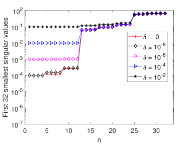
(a) Singular values based on $\mathcal{\overline{S}}^{(15,15)}_{\Omega}$.

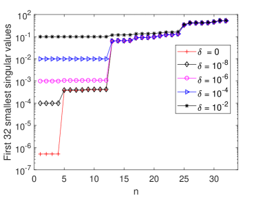
(b) Singular values based on $\mathcal{S}^{(15,15)}_{\Omega}$.

Figure 3: The first 32 singular values of the matrix (29) based on different densities of the collocation point sets $\mathcal{\overline{S}}^{(p,q)}_{\Omega}$ (see (10)) and $\mathcal{S}^{(p,q)}_{\Omega}$ (see (11)), where $\Omega=\{(x,y)|x^{2}+y^{2}\leq 0.76^{2}\}$, $\Omega_{\Box}=(-1,1)^{2}$, $N_{x}=N_{y}=4$, and $\lambda=10^{4}$.

There are a number of methods documented in the literature for solving the LS problem (17), even if (17) is ill-conditioned [24, 25]. The constrained formulation (17) can be solved by quadratic programming techniques or by writing the optimality conditions as a linear system with symmetric indefinite matrix, as follows:

$$\left[\begin{array}[]{ccc}{\mathbf{I}}&{-(\mathbf{A}_{in}-\nu\mathbf{S}_{in})}&{\mathbf{0}}\\ {-(\mathbf{A}_{in}-\nu\mathbf{S}_{in})^{T}}&{-\delta\mathbf{I}}&{(\mathbf{A}_{b})^{T}}\\ {\mathbf{0}}&{\mathbf{A}_{b}}&{\mathbf{0}}\end{array}\right]\left[\begin{array}[]{l}{\mathbf{r}}\\ {\mathbf{d}}\\ {\mathbf{\gamma}}\end{array}\right]=\left[\begin{array}[]{c}{-\mathbf{f}_{in}}\\ {-\delta\mathbf{d}^{*}}\\ \mathbf{u}_{b}\end{array}\right],$$ (30)

where $\gamma$ is a vector of Lagrange multipliers for the constraints in (17). In the numerical simulations below, we show that the constrained formulation (17) and penalized formulation (18) yield numerical solutions of similar accuracy. In the following, we discuss how to solve the unconstrained LS problem (18), which is extended to solve time-fractional PDEs in Section 3.

The solution of (18) can be obtained by forming and solving its normal equations, which are as follows:

$$((\mathbf{A}_{in}-\nu\mathbf{S}_{in})^{T}(\mathbf{A}_{in} -\nu\mathbf{S}_{in})+\lambda^{2}\mathbf{A}_{b}^{T}\mathbf{A}_{b}+\delta\mathbf{I})\mathbf{c}$$ (31)

$$=(\mathbf{A}_{in}-\nu\mathbf{S}_{in})^{T}\mathbf{f}_{in}+\lambda^{2}\mathbf{A}_{b}^{T}\mathbf{u}_{b}+\delta\mathbf{d_{*}}.$$

The condition number of the coefficient matrix in this system is approximately ${\sigma^{2}_{\max}}/{\delta}$. Iterative methods such as conjugate gradients can be used to solve (31), or it can be solved directly using a Cholesky factorization. Even when the linear system (31) is ill-conditioned, it is still possible to obtain accurate solutions with an appropriate choice of algorithms [26, 27, 24, 25]. However, our computational experiments show that those methods for solving (31) are slower than methods that apply a QR factorization directly to the matrix in (18); see Table 1. The QR-based approach can be implemented compactly by means of the backslash operator in Matlab.

2.3 Error analysis

Let $\mathbf{c}$, $\mathbf{c}_{\lambda}$, $\mathbf{c}_{\delta}$, and $\mathbf{c}_{\lambda,\delta}$ be the solutions of (14), (16), (17), and (18), respectively. Our goal in this section is to estimate the difference norm $\|\mathbf{c}-\mathbf{c}_{\lambda,\delta}\|$ between the regularized solution $\mathbf{c}_{\lambda,\delta}$ and the true solution $\mathbf{c}$.

Assume that the rank of the matrix $\mathbf{A}_{in}-\nu\mathbf{S}_{in}$ is $M$. Then the error bounds $\|\mathbf{c}-\mathbf{c}_{\lambda}\|$ and $\|\mathbf{c}_{\delta}-\mathbf{c}_{\lambda,\delta}\|$ can be derived directly from [23, equation (2.20)]. We have

$$\|\mathbf{c}-\mathbf{c}_{\lambda}\|\leq\frac{1}{2\lambda\beta_{\min}}\sqrt{\|\mathbf{r}_{\lambda}\|^{2}-\|\mathbf{r}\|^{2}},$$ (32)

where $\beta_{\min}$ is the smallest singular value of $\mathbf{A}_{b}$ and

$$\mathbf{r}=\left(\mathbf{A}_{in}-\nu\mathbf{S}_{in}\right)\mathbf{c}-\mathbf{f}_{in},{\qquad}\mathbf{r}_{\lambda}=\mathbf{A}_{\lambda}\mathbf{c}_{\lambda}-\mathbf{b}_{\lambda},$$

with $\mathbf{A}_{\lambda}=\left(\begin{array}[]{c}\mathbf{A}_{in}-\nu\mathbf{S}_{in}\\ \lambda\mathbf{A}_{b}\\ \end{array}\right)$ and $\mathbf{b}_{\lambda}=\left(\begin{array}[]{c}\mathbf{f}_{in}\\ \lambda\mathbf{u}_{b}\\ \end{array}\right)$. Numerical simulations show that $\mathbf{c}_{\lambda}$ is a good approximation of $\mathbf{c}$ for a sufficiently large value $\lambda>0$, that is, $\mathbf{c}_{\lambda}$ is bounded if $\mathbf{c}$ is bounded; see [23].

Next, we estimate $\mathbf{c}_{\lambda}-\mathbf{c}_{\lambda,\delta}$. We denote by $\hat{\sigma}_{i}$ the singular values of $\mathbf{A}_{\lambda}$, with $0<\hat{\sigma}_{\min}=\hat{\sigma}_{M}\leq\hat{\sigma}_{M-1}\leq\cdots\leq\hat{\sigma}_{1}$. Then there exist orthogonal matrices $\mathbf{U}$ and $\mathbf{V}$ such that $\mathbf{A}_{\lambda}=\mathbf{U}\Sigma\mathbf{V}^{T}$, where $\Sigma=\mathrm{diag}(\hat{\sigma}_{1},\hat{\sigma}_{2},\dotsc,\hat{\sigma}_{M})$, $\mathbf{U}=(\mathbf{u}_{1},\mathbf{u}_{2},\dotsc,\mathbf{u}_{M})$, $\mathbf{V}=(\mathbf{v}_{1},\mathbf{v}_{2},\dotsc,\mathbf{v}_{M})$, satisfying $\mathbf{U}^{T}\mathbf{U}=\mathbf{V}^{T}\mathbf{V}=\mathbf{I}$. The LS solutions of (16) and (18) can be expressed by

$$\mathbf{c}_{\lambda} =(\mathbf{A}_{\lambda}^{T}\mathbf{A}_{\lambda})^{-1}\mathbf{A}_{\lambda}^{T}\mathbf{b}_{\lambda},$$

$$\mathbf{c}_{\lambda,\delta} =(\mathbf{A}_{\lambda}^{T}\mathbf{A}_{\lambda}+\delta\mathbf{I})^{-1}\left(\mathbf{A}_{\lambda}^{T}\mathbf{b}_{\lambda}+\delta\mathbf{d}_{*}\right).$$

From the above two equations and $\mathbf{A}_{\lambda}=\mathbf{U}\Sigma\mathbf{V}^{T}$, we have

$$\|\mathbf{c}_{\lambda}-\mathbf{c}_{\lambda,\delta}\| =\|(\mathbf{A}_{\lambda}^{T}\mathbf{A}_{\lambda})^{-1}\mathbf{A}_{\lambda}^{T}\mathbf{b}_{\lambda}-(\mathbf{A}_{\lambda}^{T}\mathbf{A}_{\lambda}+\delta\mathbf{I})^{-1}\left(\mathbf{A}_{\lambda}^{T}\mathbf{b}_{\lambda}+\delta\mathbf{d}_{*}\right)\|$$ (33)

$$=\delta\|(\mathbf{A}_{\lambda}^{T}\mathbf{A}_{\lambda})^{-1}(\mathbf{A}_{\lambda}^{T}\mathbf{A}_{\lambda}+\delta\mathbf{I})^{-1}\mathbf{A}_{\lambda}^{T}\mathbf{b}_{\lambda}-(\mathbf{A}_{\lambda}^{T}\mathbf{A}_{\lambda}+\delta\mathbf{I})^{-1}\mathbf{d}_{*}\|$$

$$=\delta\|\Sigma^{-1}(\Sigma^{2}+\delta\mathbf{I})^{-1}\mathbf{U}^{T}\mathbf{b}_{\lambda}-(\Sigma^{2}+\delta\mathbf{I})^{-1}\mathbf{V}^{T}\mathbf{d}_{*}\|$$

$$\leq\delta\sum_{i=1}^{M}\left(\frac{|\mathbf{u}_{i}^{T}\mathbf{b}_{\lambda}|}{\hat{\sigma}_{i}(\hat{\sigma}_{i}^{2}+\delta)}+\frac{|\mathbf{v}_{i}^{T}\mathbf{d}_{*}|}{(\hat{\sigma}_{i}^{2}+\delta)}\right).$$

This bound shows that $\mathbf{c}_{\lambda,\delta}$ converges to $\mathbf{c}_{\lambda}$ as $\delta\to 0$, but it does not show the effectiveness of $\mathbf{d}_{*}$ in improving the accuracy of the numerical solutions. However, by writing $\mathbf{c}_{\lambda}$ as $\mathbf{c}_{\lambda}=(\mathbf{A}_{\lambda}^{T}\mathbf{A}_{\lambda}+\delta\mathbf{I})^{-1}\left(\mathbf{A}_{\lambda}^{T}\mathbf{b}+\delta\mathbf{c}_{\lambda}\right)$, we obtain

$$\|\mathbf{c}_{\lambda}-\mathbf{c}_{\lambda,\delta}\|=\delta\|(\mathbf{A}_{\lambda}^{T}\mathbf{A}_{\lambda}+\delta\mathbf{I})^{-1}\left(\mathbf{c}_{\lambda}-\mathbf{d}_{*}\right)\|\leq\frac{\delta}{\delta+\hat{\sigma}^{2}_{\min}}\|\mathbf{c}_{\lambda}-\mathbf{d}_{*}\|.$$ (34)

By combing (32) and (34), we obtain

$$\|\mathbf{c}-\mathbf{c}_{\lambda,\delta}\|\leq\frac{1}{2\lambda\beta_{\min}}\sqrt{\|\mathbf{r}_{\lambda}\|^{2}-\|\mathbf{r}\|^{2}}+\frac{\delta}{\delta+\hat{\sigma}^{2}_{\min}}\|\mathbf{c}_{\lambda}-\mathbf{d}_{*}\|.$$ (35)

This bound shows that a relatively large value of $\delta$ can be chosen to balance the accuracy and well conditioning of the LS system (18) when $\mathbf{d}_{*}$ is close to $\mathbf{c}_{\lambda}$. Even if the matrix $\mathbf{A}_{\lambda}$ is singular, highly accurate numerical solutions can still be obtained, as we show in Sections 2.4 and 4.

2.4 Examples

We present an example to show the effectiveness of methods based on the formulations (17), (18), (25), and (26) for solving a model problem on three irregular domains, including a nonconvex domain. We compare QR decomposition for solving the unconstrained LS formulation with solution of the KT system (30) that arises from the constrained LS formulation. Our results show that both methods achieve a similar level of accuracy, while the method based on QR factorization is slightly more efficient.

Example 2.1.

Solve (1) subject to suitable Dirichlet boundary conditions and a source term $f(x,y)$, such that the solution of (1) is

$$u(x,y)=\exp(x+y).$$

This problem is solved on the domains defined by the following three cases.

• Case I: the circular domain $\Omega=\{(x,y)|x^{2}+y^{2}<1\}$, see Figure 1(b).

• Case II: the irregular domain $\Omega$ defined as shown in Figure 1(c) with the boundary defined by the B-spline interpolation using the Matlab function spline$(\mathbf{x,y})$, where

  $$\mathbf{x}=\left[\begin{array}[]{cccccccccc}0&\pi/2&\pi&3\pi/2&2\pi\end{array}\right],$$

  $$\mathbf{y}=\left[\begin{array}[]{cccccccccc}0&1&0&-1&0&1&0\\ 1.7&0.9&1.8&0.5&-0.7&0.9&1.7\\ \end{array}\right].$$

• Case III : the irregular domain $\Omega$ defined as shown in Figure 1(d) with the boundary defined by the Matlab function spline$(\mathbf{x,y})$, where

  $$\mathbf{x}=\left[\begin{array}[]{cccccccccc}0&2\pi/7&4\pi/7&6\pi/7&8\pi/7&10\pi/7&12\pi/7&2\pi\end{array}\right],$$

  $$\mathbf{y}=\left[\begin{array}[]{cccccccccc}0&1&0.5&0&-0.5&-1&-0.4&0&1&0\\ 1.7&0.9&1.051&1.708&0.791&0.511&-0.107&0.296&0.9&1.7\\ \end{array}\right].$$

• Case IV : The irregular domain with oscillatory boundaries defined by the Matlab function interp1q$(\mathbf{x,y,x_{i}})$, where

  $$\mathbf{x}=\left[\begin{array}[]{cccccccccccccccc}1&&-1&&-1&&1&&1/2&&1&&0&&1\end{array}\right],$$

  $$\mathbf{y}=\left[\begin{array}[]{cccccccccccccccc}1&&1&&-1&&-1&&-1/2&&0&&\Lambda&&1\\ \end{array}\right];$$

  see Figure 4(a) for $\Lambda=1/2$ and Figure 4(b) for $\Lambda=3/4$.

  

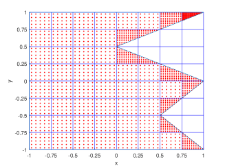
  (a) $\Lambda=1/2$.

  

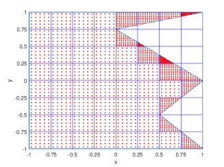
  (b) $\Lambda=3/4$.

  Figure 4: The irregular domain with oscillatory boundaries.

The $L^{2}$ error is measured by

$$\|e\|=\left(h_{x}h_{y}\sum_{i=0}^{200}\sum_{j=0}^{200}|e_{i,j}|^{2}\right)^{1/2},$$

where $e_{i,j}=u(\hat{x}_{i},\hat{y}_{j})-U_{h}(\hat{x}_{i},\hat{y}_{j})$ for $(\hat{x}_{i},\hat{y}_{j})\in\bar{\Omega}$ and $e_{i,j}=0$ for $(\hat{x}_{i},\hat{y}_{j})\notin\Omega$, $\hat{x}_{i}=a+i\hat{h}_{x}$, $\hat{y}_{j}=-c+j\hat{h}_{y}$, $\hat{h}_{x}=(b-a)/200$, and $\hat{h}_{y}=(d-c)/200$.

The default solver for the unconstrained LS problems (18) and (26) is the QR decomposition, implemented via the backslash operator “$\setminus$” in Matlab 2018a) with $\lambda=10^{5}$. We take $\nu=0.1$ and $N_{x}=N_{y}=N$ in the numerical simulations. The nonuniformly distributed collocation point set $\mathcal{S}^{(10,10)}_{\Omega}$ is used in the four methods (17), (25), (18), and (26), unless specified otherwise.

The choice of $\mathbf{d_{*}}$ in the formulations (17), (18), (25), and (26) is as follows. First, we let $\delta=\delta_{0}=10^{-6}$ and $\mathbf{d}_{*}=\mathbf{0}$ in (18) and solve it by QR factorization. The solution is denoted as $\mathbf{d}^{*}$. Then, we take $\mathbf{d_{*}}=\mathbf{d}^{*}\cdot(1+\epsilon\mathbf{\tilde{d}})$, where $\epsilon$ is a nonnegative number and $\mathbf{\tilde{d}}$ is a random vector generated by Matlab function rand. (Call rng$(1)$ before calling $\mathbf{\tilde{d}}=\texttt{rand}(M,1)$ to derive the same value of $\mathbf{\tilde{d}}$ each time the code is run.)

We show first how $\delta$ and $\epsilon$ affect the accuracy of the LSC method (18) for Case I. In Figure 5(a), we fix $\epsilon=0.01$ and see that the accuracy increases as $\delta$ decreases. Second-order accuracy is observed for smaller $\delta=2^{-4},2^{-8}$, and $2^{-12}$. In Figure 5(b), we fix $\delta=0.01$ and see that the error decreases as $\epsilon$ decreases. Second-order accuracy is observed for $\epsilon=10^{-2}$ and $10^{-3}$.

Figure 6 shows the relative $L^{2}$ errors obtained from the LSC formulation (18) for Case II. We can see that decreasing $\delta$ or $\epsilon$ improves the accuracy, and second-order is observed for smaller values of these parameters.

On the nonconvex domain of Case III, we still observe similar results as for Cases I and II; see Figure 7(b). In Figures 7(a1)-(a3), we also show the errors of the LSC method (18) based on uniformly distributed collocation points of different densities. The LSC method works less well when there are insufficient collocation points in the boundary cells; see Figure 7(a1). As the number of collocation points in the boundary cells increases, better results are obtained; see Figures 7(a2)-(a3). We conclude from these results that sufficient collocation points in the boundary cells are needed to achieve second-order accuracy, and that adding more collocation points to the inner cells of $\Omega$ does not necessarily improve the accuracy of the method. In the following, we will use the LSC method or LSFVM based on nonuniformly distributed collocation points to solve the considered differential equations.

For Case IV, we solve the problem on the domain with oscillatory boundaries. Figure 8 shows that decreasing $\epsilon$ increases accuracy, and second-order accuracy is observed for $\epsilon=10^{-4}$, which is similar to that exhibited in Figure 6 (b).

Table 1 shows the relative $L^{2}$ errors and the corresponding computational time of two approaches for Case III: QR decomposition applied to the penalized linear-least-squares formulation (18), and direct solution of the KKT conditions (30) for the constrained formulation (17). Both solvers achieve results of identical accuracy, but the method based on QR decomposition appears to be slightly more efficient, especially when the matrix is large.

Table 2 compares the LSC method (18) with the LSFVM (26). The two approaches attain similar levels of accuracy for $\rho=10^{-4}$, which is in line with the theoretical analysis in Section 2.2.2. The results in Table 2 also suggest that the LSFVM reduces to the LSC method when $\rho\to 0$.

The constrained formulation (17) (or (25)) yielded similar results as those from (18) (or (26)) for $\lambda=10^{5}$, these results are not shown here.

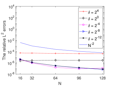
(a) $\epsilon=0.01$

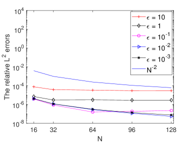
(b) $\delta=0.01$

Figure 5: The relative $L^{2}$ error $\|e\|/\|u\|$ of the LSC method (18), Example 2.1, Case I.

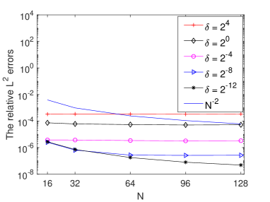
(a) $\epsilon=0.01$

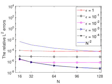
(b) $\delta=0.01$

Figure 6: The relative $L^{2}$ error $\|e\|/\|u\|$ of the LSC method (18), Example 2.1, Case II.

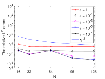
(a1) $p=q=10$.

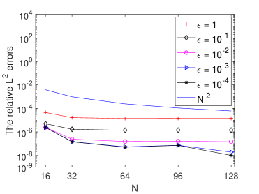
(a2) $p=q=16$.

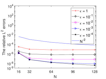
(a3) $p=q=24$.

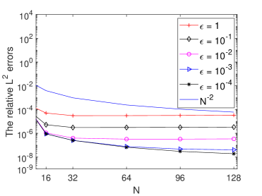
(b)

Figure 7: The relative $L^{2}$ errors $\|e\|/\|u\|$ of the LSC method (18), Example 2.1, Case III, $\delta=0.01$. (a1), (a2), and (a3) : the LS method based on the uniformly distributed collocation point set $\mathcal{\overline{S}}^{(p,q)}_{\Omega}$; (b) the LS method (18) based on non-uniformly distributed collocation point set $\mathcal{S}^{(10,10)}_{\Omega}$.

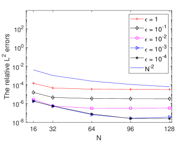
(a) $\Lambda=1/2$.

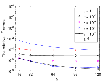
(b) $\Lambda=3/4$

Figure 8: The relative $L^{2}$ errors $\|e\|/\|u\|$ of the LSC method (18) based on non-uniformly distributed collocation point set $\mathcal{S}^{(10,10)}_{\Omega}$, Example 2.1, Case IV, $\delta=0.01$.

Table 1: The relative errors $\|e\|/\|u\|$ and computation times for a QR-based solver applied to the formulation (18) and direct solution of the KKT system (30) on Example 2.1, Case III, $\delta=\epsilon=10^{-4}$.

Method	$N=32$	Time (s)	$N=64$	Time (s)	$N=128$	Time (s)
QR, (18)	2.5601e-7	1.5560e-2	6.8002e-8	5.0821e-2	1.6083e-8	2.0375e-1
KKT, (30)	2.5601e-7	2.3683e-2	6.8002e-8	9.2296e-2	1.6083e-8	4.5509e-1

Table 2: Comparison of the relative $L^{2}$ difference $\|e\|/\|u\|$ between the LCM method (18) and the LSFVM (26), Example 2.1, Case II, $\delta=0.01$, and $N=64$.

		$\epsilon=1$	$\epsilon=10^{-2}$	$\epsilon=10^{-4}$
LSC	$-$	6.8916e-5	6.2460e-7	1.8022e-7
	$\rho=10^{-4}$	6.8916e-5	6.2462e-7	1.8011e-7
	$\rho=10^{-3}$	6.8879e-5	6.2656e-7	1.6937e-7
LSFVM	$\rho=10^{-2}$	6.1956e-5	1.3875e-6	9.0710e-7
	$\rho=2\times 10^{-2}$	7.3184e-5	4.5220e-6	4.1602e-6
	$\rho=10^{-1}$	1.5751e-4	1.0895e-4	1.0873e-4

One further example shows that the Neumann boundary conditions can be handled easily in the present framework.

Example 2.2.

Consider (1) subject to the following Neumann boundary conditions

$$\mathcal{B}(u)=(\mathbf{\hat{n}}\cdot\nabla u)(x,y)=u_{b}(x,y),\quad(x,y)\in\partial\Omega,$$ (36)

where $\mathbf{\hat{n}}=(\hat{n}_{x},\hat{n}_{y})^{T}$ denotes the unit normal to the outer boundary of $\Omega$.

In a similar fashion to (12), (13), we obtain the following overdetermined system:

$$\left\{\begin{aligned} &\left(\Phi^{T}\mathbf{d}-\nu\Delta\Phi^{T}\mathbf{d}\right)(\xi^{(in)}_{i})-f(\xi^{(in)}_{i})=0,{\quad}1\leq i\leq N_{in},\\ &\left(\Phi^{T}\mathbf{d}-\nu\Delta\Phi^{T}\mathbf{d}\right)(\xi^{(b)}_{i})-f(\xi^{(b)}_{i})-\widetilde{\lambda}\left(\mathcal{B}(\Phi^{T}\mathbf{d})-u_{b}\right)(\xi^{(b)}_{i})=0,{\quad}1\leq i\leq N_{b},\end{aligned}\right.$$ (37)

where the Neumann boundary conditions (the second equation in (37)) are imposed according to [28, equation (28)]. The parameter $\widetilde{\lambda}$ is a positive constant dependent on the mesh, which is chosen as $\widetilde{\lambda}=4\max\{(b-a)N_{x},(d-c)N_{y}\}$ in the numerical simulations in this work; see [28, Section 4.1.4].

The penalized LSC method for (1) subject to the Neumann boundary condition (36) is given by

$$\mathbf{c} =\arg\min_{\mathbf{d}\in\mathbb{R}^{M}}\left\|\left(\begin{array}[]{c}\mathbf{A}_{in}-\nu\mathbf{S}_{in}\\ \mathbf{A}_{b}-\nu\mathbf{S}_{b}-\widetilde{\lambda}\mathbf{B}\\ \sqrt{\delta}\mathbf{I}\\ \end{array}\right)\mathbf{d}-\left(\begin{array}[]{c}\mathbf{f}_{in}\\ \mathbf{f}_{b}-\widetilde{\lambda}\mathbf{u}_{b}\\ \sqrt{\delta}\mathbf{d_{*}}\\ \end{array}\right)\right\|^{2},$$ (38)

where $\mathbf{B}$ is related to $(\mathbf{\hat{n}}\cdot\nabla U_{h})(x,y)$ (We avoid an explicit specification here).

We apply (38) to solve (1) subject to the Neumann boundary condition (36) on the circular domain (see Figure 1(b) and Case I in Example 2.1) and the irregular domain (see Figure 1(c) and Case II in Example 2.1). Relative errors are shown in Figure 9. Note that second-order accuracy is still observed for small $\epsilon$.

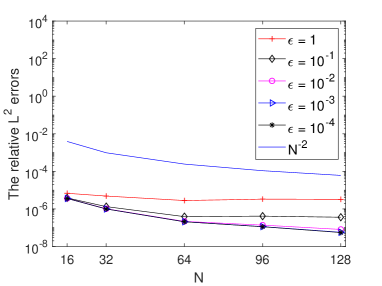
(a) The circular domain in Case I

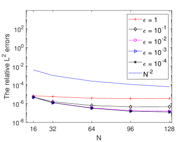
(b) The irregular domain in Case II

Figure 9: Relative errors of the LSC method (38) subject to the Neumann boundary conditions (36), compared to the the exact solution $u=\exp(x+y)$, Example 2.2, $\nu=0.1$, $\delta=0.0001$, $\widetilde{\lambda}=4\max\{(b-a)N,(d-c)N\}$.

3 Application to nonlinear time-dependent models

In this section, we extend the discrete LSC method and LSFVM to solve the following nonlinear time-fractional diffusion equation

$$\left\{\begin{aligned} &{}_{C}D^{\alpha}_{0,t}u(x,y,t)=\nu\Delta u(x,y,t)+f(u,x,y,t),{\quad}&&(x,y,t)\in\Omega\times(0,T],\\ &u(x,y,0)=\phi(x,y),{\quad}&&(x,y)\in\Omega,\\ &u(x,y,t)=u_{b}(x,y,t),{\quad}&&(x,y,t)\in\partial\Omega\times[0,T].\end{aligned}\right.$$ (39)

We apply a stable semi-implicit time-stepping method to discretize the time direction of (39) to derive a linear boundary value problem. The boundary value problem is solved by the LSC or LSFVM approaches developed in the previous section.

3.1 Semi-implicit time-stepping method

We recall a semi-implicit method proposed in [20] for the fractional initial value problem

$${}_{C}D^{\alpha}_{0,t}u(t)=\nu u(t)+f(u(t),t),{\quad}u(0)=u^{0},{\quad}t\in(0,T],$$ (40)

where $0<\alpha\leq 1$, $\nu<0$, $f(u,t)$ is a nonlinear function with respect to $u$, and the Caputo fractional operator ${}_{C}D^{\alpha}_{0,t}$ is defined by

$${}_{C}D^{\alpha}_{0,t}u(t)=\frac{1}{\Gamma(1-\alpha)}\int_{0}^{t}(t-s)^{-\alpha}u^{\prime}(s)\,{\rm d}s.$$ (41)

We assume that the solution $u(t)$ to (40) satisfies

$$u(t)-u(0)=\sum_{k=1}^{m}c_{k}t^{\gamma_{k}}+t^{\gamma_{m+1}}\tilde{u}(t),{\quad}0<\gamma_{k}<\gamma_{k+1},$$ (42)

where $\tilde{u}(t)$ is uniformly bounded for $t\in[0,T]$. This assumption holds in real applications; see for example, [29, 30, 31, 32, 33]. If $f(u(t),t)$ is smooth for $t\in[0,T]$, then $\gamma_{k}\in\{i+j\alpha,i=0,1,\dotsc;j=0,1,\dotsc\}$; see [29].

Combining (40) and (42), we obtain

$$f(u(t),t)-f(u(0),0)={}_{C}D^{\alpha}_{0,t}u(t)-\nu u(t)=\sum_{k=1}^{m_{f}}\hat{c}_{k}t^{\hat{\gamma}_{k}}+t^{\hat{\gamma}_{k+1}}v(t),$$ (43)

where $0<\hat{\gamma}_{k}<\hat{\gamma}_{k+1}$, $\hat{\gamma}_{k}\in\{\gamma_{k}\}\cup\{\gamma_{k}-\alpha\}$, and $v(t)$ is bounded for $t\in[0,T]$.

Denote by $t_{j}=j\tau\,(j\geq 0)$ the grid points, where $\tau=T/n_{T}$ is the stepsize and $n_{T}$ is a positive integer. Let $u^{n}=u(t_{n})$ and denote

$$D_{\tau}^{(\alpha,n,m,\gamma)}u=\frac{1}{\tau^{\alpha}}\sum_{j=0}^{n}\omega^{(\alpha)}_{n-j}(u^{j}-u^{0})+\frac{1}{\tau^{\alpha}}\sum_{j=1}^{m}w^{(\alpha)}_{n,j}(u^{j}-u^{0}),$$ (44)

where $m\geq 0$ is the number of correction terms and the quadrature weights $\omega^{(\alpha)}_{j}$ satisfy

$$\omega^{(\alpha)}(z)=(1-z)^{\alpha}\left(1+\frac{\alpha}{2}-\frac{\alpha}{2}z\right)=\sum_{n=0}^{\infty}\omega^{(\alpha)}_{n}z^{n}.$$ (45)

The starting weights $\{w^{(\alpha)}_{n,j}\}$ are chosen such that

$$\sum_{j=0}^{n}\omega^{(\alpha)}_{n-j}u^{j}+\sum_{j=1}^{m}w^{(\alpha)}_{n,j}u^{j}=\frac{\Gamma(\gamma_{k}+1)}{\Gamma(\gamma_{k}+1-\alpha)}n^{\gamma_{k}-\alpha}$$

for some $u(t)=t^{\gamma_{k}}\,(0<\gamma_{k}<\gamma_{k+1})$. (We refer readers to [34, 35, 36] for further information on calculation and properties of the starting weights.)

We also introduce the notation $E^{(n,m,\gamma)}_{2}$ defined by

$$E^{(n,m,\sigma)}_{2}(u)=u^{n}-2u^{n-1}+u^{n-2}-\sum_{j=1}^{m}w^{(u)}_{n,j}(u^{j}-u^{0}),$$ (46)

where $\{w^{(u)}_{n,j}\}$ are chosen such that $E^{(n,m,\gamma)}_{2}(u)=0$ for $u=t^{\gamma_{r}}$ $(0<\gamma_{r-1}<\gamma_{r})$.

By applying the second-order semi-implicit time-stepping method proposed in [20, equation (17)] to discretize (40), we obtain

$$D_{\tau}^{(\alpha,n,m,\gamma)}u=\nu u^{n}+f^{n}-E^{(n,m_{f},\hat{\gamma})}_{2}(f)-\kappa E^{(n,m_{u},\gamma)}_{2}(u)+R^{n},$$ (47)

where $f^{n}=f(u^{n},t_{n})$, $\kappa$ is a constant that balances the stability and accuracy of method (47), and $R^{n}$ is the time discretization error satisfying

$$R^{n}=O(\tau^{2}t_{n}^{\gamma_{m+1}-2-\alpha})+O(\tau^{2}t_{n}^{\hat{\gamma}_{m_{f}+1}-2})+O(\tau^{2}t_{n}^{\gamma_{m_{u}+1}-2}).$$ (48)

Remark 3.1.

Generally speaking, the solution of (40) has singularity at $t=0$ due to the singularity of the kernel in the fractional derivative operator (41), which may lead to low accuracy of some numerical methods [29]. In this work, we use the correction ${\tau^{-\alpha}}\sum_{j=1}^{m}w^{(\alpha)}_{n,j}(u^{j}-u^{0})$ to preserve high accuracy of the time-stepping method (44) for the approximation of ${}_{C}D^{\alpha}_{0,t}u(t)$. If $u(t)$ satisfies (43) and $\gamma_{1}<1$, then $E^{(n,0,\sigma)}_{2}(u)=u^{n}-2u^{n-1}+u^{n-2}=O(\tau^{2}t_{n}^{\gamma_{1}-2})=O(\tau^{\gamma_{1}})$ for a small $n$, which yields large discretization error of (47). We also use the correction terms to achieve $E^{(n,m_{u},\sigma)}_{2}(u)=O(\tau^{2})$ for all $n>0$ when $\gamma_{m_{u}+1}\geq 2$ (see (48)). See [34, 35, 36, 20] for more details.

3.2 The fully discrete scheme

We apply the time-stepping method (47) to discretize the time direction of (39) and obtain the following semi-discrete scheme: For all $n>\max\{m,m_{u},m_{f}\}$, find $U^{n}=U^{n}(x,y)$ such that

$$D_{\tau}^{(\alpha,n,m,\gamma)}U=\nu\Delta U^{n}+F^{n}-E^{(n,m_{f},\hat{\gamma})}_{2}(F)-\kappa E^{(n,m_{u},\gamma)}_{2}(U),$$ (49)

where $F^{n}=f(x,y,U^{n},t_{n})$, $\kappa$ is a nonnegative constant. (Nonnegative $\kappa$ helps to enhance the stability of (49).) The method (49) is unconditionally stable for $\tau>0$ if $\kappa>0.75\max|\partial_{u}f|$; see [20, Theorem 3] and its numerical verification. In real applications, $\kappa$ can be estimated. For example, we can apply the fully implicit method with coarse grid to solve (40) to get an approximation of $u$, and use this approximation to estimate $\max|\partial_{u}f|$.

Rewriting (49) as the following linear boundary value problem

$$\left\{\begin{aligned} &\left(\omega_{0}^{(\alpha)}+\kappa\tau^{\alpha}\right)U^{n}-\nu\tau^{\alpha}\Delta U^{n}=RHS^{n-1},&(x,y)\in\Omega,\\ &U^{n}(x,y)=u_{b}(x,y,t_{n}),&(x,y)\in\partial\Omega,\end{aligned}\right.$$ (50)

where

$$RHS^{n-1}= RHS^{n-1}(x,y)=\tau^{\alpha}D_{\tau}^{(\alpha,n,m,\gamma)}U-\omega_{0}^{(\alpha)}U^{n}$$ (51)

$$+F^{n}-E^{(n,m_{f},\hat{\gamma})}_{2}(F)+\kappa(U^{n}-E^{(n,m_{u},\gamma)}_{2}(U)).$$

Let $U_{h}^{n}=\Phi^{T}(x,y)\mathbf{c}^{n}\in\mathcal{M}_{\Omega}(\delta_{x}\times\delta_{y})$ be the approximate solution of (50). By inserting $U_{h}^{n}$ into the first equation of (50) and choosing $(x,y)=\xi_{i}^{(in)}\in\mathcal{S}^{(p,q)}_{\Omega}$, we obtain

$$\left(\omega_{0}^{(\alpha)}+\kappa\tau^{\alpha}\right)U_{h}^{n}(\xi_{i}^{(in)})-\nu\tau^{\alpha}\Delta U^{n}_{h}(\xi_{i}^{(in)})=RHS^{n-1}(\xi_{i}^{(in)}),\quad 1\leq i\leq N_{in},$$ (52)

subject to the constraints

$$U_{h}^{n}(\xi^{(b)}_{i})=\Phi^{T}(\xi^{(b)}_{i})\mathbf{c}^{n}=u_{b}(\xi^{(b)}_{i},t_{n}),{\quad}1\leq i\leq N_{b}.$$ (53)

As in (18), the discrete LS solution of (52)–(53) is approximated by

$$\mathbf{c}^{n} =\arg\min_{\mathbf{d}\in\mathbb{R}^{M}}\left\|\left(\begin{array}[]{c}(\omega_{0}^{(\alpha)}+\kappa\tau^{\alpha})\mathbf{A}_{in}-\nu\tau^{\alpha}\mathbf{S}_{in}\\ \lambda\mathbf{A}_{b}\\ \sqrt{\delta}\mathbf{I}\\ \end{array}\right)\mathbf{d}-\left(\begin{array}[]{c}\mathbf{RHS}^{n-1}_{in}\\ \lambda\mathbf{u}_{b}^{n}\\ \sqrt{\delta}\mathbf{d}^{n}_{*,r}\\ \end{array}\right)\right\|,$$ (54)

where $\mathbf{A}_{in}$, $\mathbf{A}_{b}$, and $\mathbf{S}_{in}$ are defined in (15), $\delta\geq 0$, $\mathbf{RHS}^{n-1}_{in}$ is a vector whose $i$th component is ${RHS}^{n-1}(\xi^{(in)}_{i})$; $\mathbf{d}^{n}_{*,r}$ is a reference solution, chosen such that $\|\mathbf{c}^{n}-\mathbf{d}^{n}_{*,r}\|$ is suitably small; and $\lambda$ is the positive weight parameter that controls fidelity to the boundary conditions. We choose the reference solution $\mathbf{d}^{n}_{*,r}$ to be

$$\mathbf{d}^{n}_{*,r}=\left\{\begin{aligned} &\mathbf{0},{\qquad\qquad}r=0,\\ &\mathbf{c}^{n-1},{\qquad\,\,\,}r=1.\end{aligned}\right.$$ (55)

The choice of $\mathbf{d}^{n}_{*,r}$ is inspired by the relation $\|\mathbf{c}^{n}-\mathbf{d}^{n}_{*,r}\|=O(\tau^{r})$ observed from the time-stepping methods for solving time-dependent problems, which is numerically verified in our computational results of the next section.

The LSFVM for (52) can be obtained similarly, where we replace the matrices $\mathbf{A}_{in}$ and $\mathbf{S}_{in}$ in (54) with $\mathbf{\widetilde{A}}_{in}$ and $\mathbf{\widetilde{S}}_{in}$, respectively, where $\mathbf{\widetilde{A}}_{in}$ and $\mathbf{\widetilde{S}}_{in}$ are defined in (24).

4 Numerical examples and applications

We present Examples 4.1 and 4.2, to display the efficiency of the LSC method (54). For each example, we consider two different cases based on a known solution with a source term and an unknown solution with zero source but oscillating initial conditions. Since LSFVM gives similar results to the LSC when $\rho$ is suitably small, we do not discuss the results of LSFVM further.

The following four different domains are considered for Example 4.1.

• the rectangular domain $\Omega=(-1,1)\times(-1,1)$, see Figure 1(a);

• the circular domain $\Omega=\{(x,y)|x^{2}+y^{2}<1\}$, see Figure 1(b);

• the irregular domain $\Omega$ defined by Figure 1(c), see Case II in Example 2.1;

• the irregular domain $\Omega$ defined by Figure 1(d), see Case III in Example 2.1.

We consider Example 4.2 on the irregular domain (iv).

Example 4.1.

Consider the following nonlinear equation

$${}_{C}D^{\alpha}_{0,t}u(x,y,t)=\Delta u(x,y,t)+u(1-u^{2})+g(x,y,t),{\quad}(x,y,t)\in\Omega\times(0,T],$$ (56)

subject to suitable initial and Dirichlet boundary conditions.

The following two cases are considered in this example.

• Case I: Choose initial and boundary conditions, and source term $g(x,y,t)$, such that the analytical solution of (56) is

  $$u(x,y,t)=E_{\alpha}(-t^{\alpha})\sin(x)\sin(y).$$ (57)

• Case II: Choose initial value $u(x,y,0)=\sin(\pi x)\sin(\pi y)$, source term $g=0$, and homogenous boundary conditions.

We always choose $m_{f}=m_{u}=m$ with correction indices $\gamma_{k}=k\alpha$ (see [20, 36] and (43) for choosing $\hat{\gamma}_{k}$), $\lambda=10^{5}$, and $N_{x}=N_{y}=N$ when (56) is solved by (54). If (56) is solved on the rectangular domain, then (54) is relatively well-conditioned, so we take $\delta=0$ in the computation. When $\alpha=1$, this model reverts to a standard diffusion equation.

We verify the accuracy of the LSC method (54) in Case I, where the analytical solution is given explicitly on four different domains. Tables 3 shows relative $L^{2}$ errors for this approach at $t=2$ on the rectangular domain. Second-order accuracy is observed once again.

Table 3: The $L^{2}$ error $\|e^{n}\|$ of the LSC method (54) at $t=2$ on the rectangular domain (i), Example 4.1, Case I, with $\kappa=2$, $\gamma_{k}=k\alpha$, $\tau=2^{-10}$.

$N$	$\alpha=0.1,m=3$	Order	$\alpha=0.5,m=3$	Order	$\alpha=0.8,m=1$	Order	${\alpha=1,m=1}$	Order
$8$	3.4971e-6		2.5365e-6		1.7604e-6		1.1468e-6
$16$	6.1913e-7	2.4979	4.5642e-7	2.4744	3.1358e-7	2.4890	1.8610e-7	2.6235
$32$	1.7198e-7	1.8480	1.2340e-7	1.8870	8.5040e-8	1.8826	4.5807e-8	2.0224
$48$	7.8119e-8	1.9463	5.4424e-8	2.0190	3.8185e-8	1.9747	1.6985e-8	2.4468
$64$	4.4314e-8	1.9707	2.9698e-8	2.1056	2.1401e-8	2.0126	6.6661e-9	3.2511

When the LSC method (54) is applied to solve (56) on irregular domains (ii)-(iv), the condition number of the coefficient matrix in (54) may be large, but regularization helps to improve the conditioning while still yielding accurate numerical solutions. Figure 10(a) shows the $L^{2}$ error of the LSC method (54) at $t=2$ on the circular domain (ii) for $r=0$. We observe second-order accuracy again for $\delta=10^{-6}$. Figure 10(b) shows these errors for $r=1$, where we observe more accurate numerical simulations even for larger values of $\delta$. (Second-order accuracy can be observed even for $\delta=10^{-2}$.) For $\delta=10^{-1}$ and $r=1$, the regularization error plays the dominant role, we observe that the error is saturated as $N$ increases up to $64$; see Figure 10(b). For $\delta=10^{-2}$ and $r=1$, the space discretization error plays the dominant role when $N\leq 32$. For $N\in(32,64]$, both the space discretization error and the regularization error play important roles; we observe in Figure 10(b) and Figure 11(b) that these errors fluctuate slightly with $N$. For the irregular domains (iii) and (iv), we observe similar results as those shown in Figure 10. Figure 11 shows the $L^{2}$ errors on the irregular domains (iii) and (iv) for $r=1$. From these figures, we can see that a relatively large $\delta$ with $r=1$ yields a well-conditioned system (54) and accurate numerical solutions, in agreement with the results in Example 2.1. In the remainder of this section, we will use $r=1$ with a relatively large value of $\delta$ in the computations.

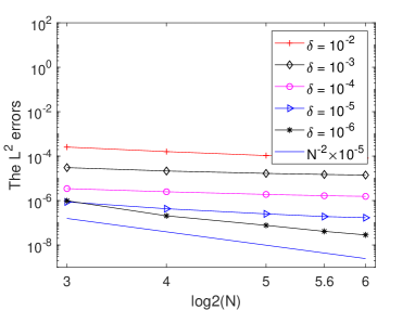
(a) $r=0$.

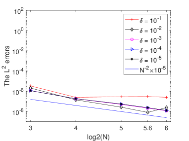
(b) $r=1$.

Figure 10: The $L^{2}$ errors at $t=2$ on the circular domain (ii), Example 4.1, Case I, $\kappa=2$, $\gamma_{k}=k\alpha$, $\alpha=0.5$, $\tau=2^{-10},m=3$.

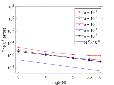
(a) Irregular domain (iii), $r=1$.

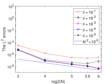
(b) Irregular domain (iv), $r=1$.

Figure 11: The $L^{2}$ errors at $t=2$ on the irregular domains (iii) and (iv), Example 4.1, Case I, $\kappa=2$, $\gamma_{k}=k\alpha$, $\alpha=0.5$, $\tau=2^{-10},m=3$.

For Case II, we obtain a proxy for the exact solution by using the LSC method (54) with $r=1$, $\delta=0.01$, and $N=64$. Figures 12(a) and (b) show the numerical solution on the rectangular domain (i) at different times $t=1$ and $t=4$. We observe that the solution decays as $t$ evolves. Comparing Figure 12(a) with Figure 12(b), we observe that the solution decays faster as $\alpha$ becomes larger. For the irregular domains defined by (ii), (iii), and (iv), we observe similar results as those shown in Figure 12 for the rectangular domain (i), see Figures 13-15.

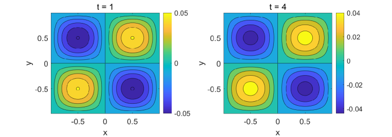
(a) $\alpha=0.2$.

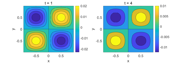
(b) $\alpha=0.8$.

Figure 12: Numerical solutions on the rectangular domain (i) for Example 4.1, Case II, $\gamma_{k}=k\alpha$, $\kappa=2,\tau=2^{-7},m=1$, $\mu=1$.

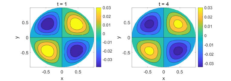
(a) $\alpha=0.2$.

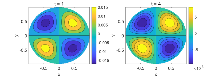
(b) $\alpha=0.8$.

Figure 13: Numerical solutions on the circular domain (ii) for Example 4.1, Case II, $\gamma_{k}=k\alpha$, $\kappa=2,\tau=2^{-7},m=1$, $\mu=1$.

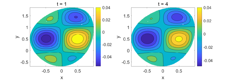
(a) $\alpha=0.2$.

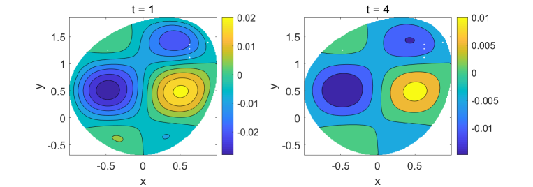
(a) $\alpha=0.8$.

Figure 14: Numerical solutions on the irregular domain (iii) for Example 4.1, Case II, $\gamma_{k}=k\alpha$, $\kappa=2,\tau=2^{-7},m=1$, $\mu=1$.

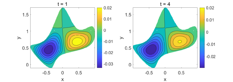
(a) $\alpha=0.2$.

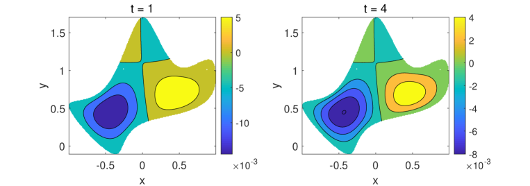
(a) $\alpha=0.8$.

Figure 15: Numerical solutions on the irregular domain (iv) for Example 4.1, Case II, $\gamma_{k}=k\alpha$, $\kappa=2,\tau=2^{-7},m=1$, $\mu=1$.

In the following example, we extend the LSC method (54) to a system of equations with different fractional indices.

Example 4.2.

Consider the following system of equations

$$\left\{\begin{aligned} &{}_{C}D^{\alpha}_{0,t}u(x,y,t)=\mu\Delta u(x,y,t)+f(x,y,t),{\quad}(x,y,t)\in\Omega_{1}\times(0,T],\\ &{}_{C}D^{\beta}_{0,t}v(x,y,t)=\nu\Delta v(x,y,t)+g(x,y,t),{\quad}(x,y,t)\in\Omega_{2}\times(0,T],\end{aligned}\right.$$ (58)

subject to suitable initial conditions and the following boundary conditions

$$\left\{\begin{aligned} &v(x,y,t)=v_{b}(x,y,t),{\qquad}&&(x,y)\in\Gamma_{2},\\ &u(x,y,t)=v(x,y,t),{\quad}\mathbf{n}\cdot\nabla u=\mathbf{n}\cdot\nabla v,{\qquad}&&(x,y)\in\Gamma_{1,2}=\partial\Omega_{1},\end{aligned}\right.$$ (59)

where, in Figure 16, $\Omega_{1}$ is the area inside the curve $\Gamma_{1,2}$ (the shaded area) and $\Omega_{2}$ is the area between the curves $\Gamma_{1,2}$ and $\Gamma_{2}$.

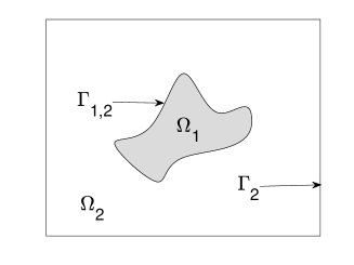
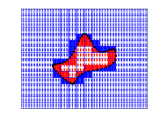
Figure 16: The domains $\Omega_{1}$ and $\Omega_{2}$ with the shared boundary $\Gamma_{1,2}$ (left) and their division and distribution of collocation points (right).

We first apply the time-stepping method (47) to each equation of (58) to obtain

$$\left\{\begin{aligned} &D_{\tau}^{(\alpha,n,m,\gamma)}u=\mu\Delta u^{n}+f^{n}+R_{1}^{n},\\ &D_{\tau}^{(\beta,n,\tilde{m},\tilde{\gamma})}v=\nu\Delta v^{n}+g^{n}+R_{2}^{n},\end{aligned}\right.$$ (60)

where $D_{\tau}^{(\alpha,n,m,\gamma)}$ is defined by (44), and $R_{1}^{n}$ and $R_{2}^{n}$ are truncation errors in time that depend on the regularity of $u$ and $v$, respectively. Omitting the truncation errors in (60), we derive the following semi-discrete method for (58):

$$\left\{\begin{aligned} &\omega_{0}^{(\alpha)}U^{n}-\mu\tau^{\alpha}\Delta U^{n}=RHS_{1}^{n-1}=\tau^{\alpha}D_{\tau}^{(\alpha,n,m,\gamma)}U-\omega_{0}^{(\alpha)}U^{n}+\tau^{\alpha}f^{n},\\ &\omega_{0}^{(\beta)}V^{n}-\nu\tau^{\beta}\Delta V^{n}=RHS_{2}^{n-1}=\tau^{\beta}D_{\tau}^{(\beta,n,\tilde{m},\tilde{\gamma})}V-\omega_{0}^{(\beta)}V^{n}+\tau^{\beta}g^{n},\end{aligned}\right.$$ (61)

subject to the boundary conditions

$$\left\{\begin{aligned} &V^{n}(x,y)=v_{b}(x,y,t_{n}),{\qquad}&&(x,y)\in\Gamma_{2},\\ &U^{n}(x,y)=V^{n}(x,y),{\quad}\mathbf{n}\cdot\nabla U^{n}=\mathbf{n}\cdot\nabla V^{n},{\qquad}&&(x,y)\in\Gamma_{1,2}=\partial\Omega_{1}.\end{aligned}\right.$$ (62)

The penalized LSC formulation of (61)–(62) is

$$\sum_{i=1}^{N^{u}_{in}}\left[J^{n}(\xi^{(in)}_{i},\mathbf{d})\right]^{2}+\sum_{i=1}^{N^{v}_{in}}\left[\hat{J}^{n}(\eta^{(in)}_{i},\mathbf{\hat{d}})\right]^{2}+\lambda^{2}\sum_{i=1}^{N^{v}_{b}}\left(R^{n}_{v}(\eta^{(b)}_{i},\mathbf{\hat{d}})\right)^{2}$$ (63)

$${\qquad}+\lambda^{2}\sum_{i=1}^{N_{c}}\left[\left(R^{n}_{u=v}(\varsigma_{i},\mathbf{d},\mathbf{\hat{d}})\right)^{2}+\left(R^{n}_{\mathbf{n}\cdot\nabla}(\varsigma_{i},\mathbf{d},\mathbf{\hat{d}})\right)^{2}\right]$$

$${\qquad}+\delta\left(\|\mathbf{d}-\mathbf{d}^{n-1}\|^{2}+\|\mathbf{\hat{d}}-\mathbf{\hat{d}}^{n-1}\|^{2}\right),$$

where $\delta\geq 0$ is the regularization parameter, $\lambda$ is the penalty parameter for the boundary conditions, $N_{in}^{u}$ and $N_{in}^{v}$ are the numbers of collocation points in $\Omega_{1}$ and $\Omega_{2}$, respectively, $N_{b}^{v}$ is the number of boundary points on $\Gamma_{2}$, $N_{c}$ is the number of boundary points on $\Gamma_{1,2}$, and

$$J^{n}(x,y,\mathbf{d}) =\omega_{0}^{(\alpha)}U^{n}_{h}(x,y)-\mu\tau^{\alpha}\Delta U^{n}_{h}(x,y)-RHS_{1}^{n-1}(x,y), (x,y)\in\Omega_{1},$$ (64)

$$\hat{J}^{n}(x,y,\mathbf{\hat{d}}) =\omega_{0}^{(\beta)}V^{n}_{h}(x,y)-\nu\tau^{\beta}\Delta V^{n}_{h}(x,y)-RHS_{2}^{n-1}(x,y), (x,y)\in\Omega_{2},$$

$$R^{n}_{v}(x,y,\mathbf{\hat{d}}) =V^{n}_{h}(x,y)-v_{b}(x,y,t_{n}), {(x,y)\in\Gamma_{2}},$$

$$R^{n}_{u=v}(x,y,\mathbf{d},\mathbf{\hat{d}}) =U^{n}_{h}(x,y)-V^{n}_{h}(x,y), (x,y)\in\Gamma_{1,2},$$

$$R^{n}_{\mathbf{n}\cdot\nabla}(x,y,\mathbf{d},\mathbf{\hat{d}}) =\mathbf{n}\cdot\nabla U_{h}^{n}-\mathbf{n}\cdot\nabla V_{h}^{n}, (x,y)\in\Gamma_{1,2},$$

with $U^{n}_{h}(x,y)=\Phi^{T}(x,y)\mathbf{d}^{n}\in\mathcal{M}_{\Omega_{1}}(\delta_{x}\times\delta_{y}),\mathbf{d}^{n}\in\mathbb{R}^{M_{u}}$ and $V^{n}_{h}(x,y)=\widehat{\Phi}^{T}(x,y)\mathbf{\hat{d}}^{n}\in\mathcal{M}_{\Omega_{2}}(\delta_{x}\times\delta_{y}),\mathbf{\hat{d}}^{n}\in\mathbb{R}^{M_{v}}$. The distribution of collocation points is shown as Figure 16 (right), which is defined similarly to $\mathcal{S}^{(p,q)}_{\Omega}$; see (10).

• Case I: Choose initial and boundary conditions, and source terms, to yield the following solution to (58)-(59):

  $$u(x,y,t) =E_{\alpha}(-t^{\alpha})\sin(3x)\sin(3y),{\quad}(x,y)\in\Omega_{1},$$

  $$v(x,y,t) =E_{\beta}(-t^{\beta})\sin(3x)\sin(3y),{\quad}(x,y)\in\Omega_{2},$$

  where $\alpha=\beta$.

• Case II: The initial conditions are taken as $u(x,y,0)=\sin(2\pi x)\sin(2\pi y)$, $(x,y)\in\bar{\Omega}_{1}$, $v(x,y,0)=\sin(2\pi x)\sin(2\pi y),(x,y)\in\bar{\Omega}_{2}$, $f=0$ for $(x,y)\in{\Omega}_{1}$, and $g=0$ for $(x,y)\in{\Omega}_{2}$.

In this example, we set $N_{x}=N_{y}=N$, $m=\tilde{m}=1$, $\gamma_{1}=\alpha$, $\tilde{\gamma}_{1}=\beta$, $\lambda=10^{5}$, and $\delta=0.01$ in the LSC method (63). The computational domain in Cases I and II satisfies $\bar{\Omega}_{1}\cup\bar{\Omega}_{2}=[-1.5,1.5]\times[-1,2]$, where $\Omega_{1}$ is defined by Figure 1(d); see also (iv) at the beginning of this section.

We show the $L^{2}$ errors of $u$ and $v$ for Case I at $t=2$ in Table 4. We can see that satisfactory numerical solutions are obtained, although the convergence rate in space is slightly less than two, due to ill conditioning in the least squares formulation.

Table 4: The $L^{2}$ error of the LSC method (63) at $t=2$, Example 4.2, Case I, $\alpha=\beta=0.5$, and $\tau=2^{-10}$.

$N$	$L^{2}$-error $(u)$	Order	$L^{2}$-error $(v)$	Order
$8$	7.7227e-4		6.9974e-4
$16$	7.3497e-5	3.3933	6.2523e-5	3.4844
$32$	2.9992e-5	1.2931	2.7286e-5	1.1962
$50$	1.3148e-5	2.0338	1.1755e-5	2.0768
$64$	8.4209e-6	1.5489	7.5325e-6	1.5471

For Case II, we do not have the the analytical solutions, so we exhibit only the numerical solutions in Figures 17 and 18. We set $\tau=2^{-7}$, $N=80$, choose oscillating initial conditions, and set the source terms to zero.

First, we fix the diffusion coefficients $\mu=\nu=1$ and see how the fractional orders $\alpha$ and $\beta$ affect the solution of (59). For $\alpha=\beta=0.2$, both the solutions $u$ (inside the black curve) and $v$ (outside the black curve) decay to two oscillating patterns as time $t$ increases; see Figure 17(a). With $\alpha=\beta$, both $u$ and $v$ decay faster to the corresponding oscillating patterns as $\alpha$ becomes larger; see Figure 17(b). When we choose a smaller $\alpha=0.2$ and a large $\beta=0.8$, we observe that $u$ decays slower than $v$; see Figure 17(c). For a larger $\alpha$ value of $0.8$ and a smaller $\beta$ value of $0.2$, we observe th faster decay of $u$ and slower decay of $v$; see Figure 17(d).

Second, we choose a larger coefficient $\mu=10$ and a smaller coefficient $\nu=1$ in the computation. For $\alpha=\beta=0.2$, we observe that $u$ decays faster than $v$ because of a larger $\mu$; see Figure 18. Closer observation reveals that increasing $\mu$ is somewhat equivalent to increasing $\alpha$, for fixed $\beta$ and $\nu$; see Figure 17(c) and Figure 18. Similar behavior is observed for $\alpha=\beta=0.8$, but $u$ (or $v$) decays faster than $u$ (or $v$) for the case $\alpha=\beta=0.2$, see Figure 18(b).

Last, we choose a smaller diffusion coefficient $\mu=1$ and a larger diffusion coefficient $\nu=10$. We observe faster decay for $v$ than for $u$ when $\alpha=\beta$ (see Figures 19(a) and (b)), due to the larger value of $\nu$. Larger values of $\alpha$ and $\beta$ (with $\alpha=\beta$) lead to faster decay of both $u$ and $v$. Compared with Figure 17(c), we observe that increasing $\nu$ is somewhat, but not precisely, equivalent to increasing the fractional order $\beta$, for fixed $\alpha$ and $\mu$.

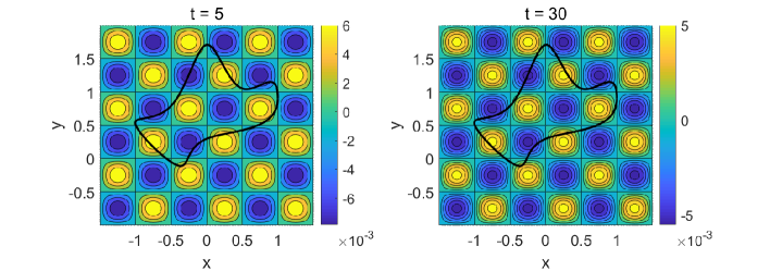
(a) $\alpha=\beta=0.2$.

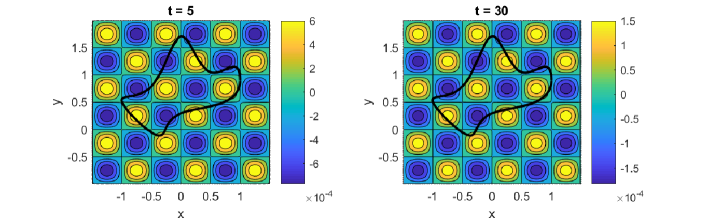
(b) $\alpha=\beta=0.8$.

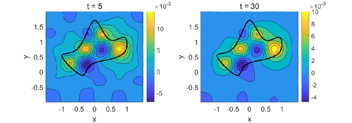
(c) $\alpha=0.2,\beta=0.8$.

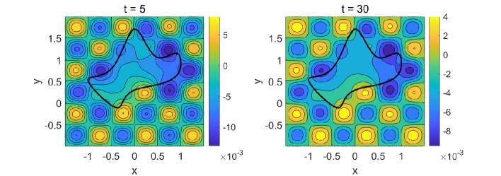
(d) $\alpha=0.8,\beta=0.2$.

Figure 17: Numerical solutions for Example 4.2, Case II, $\mu=\nu=1$.

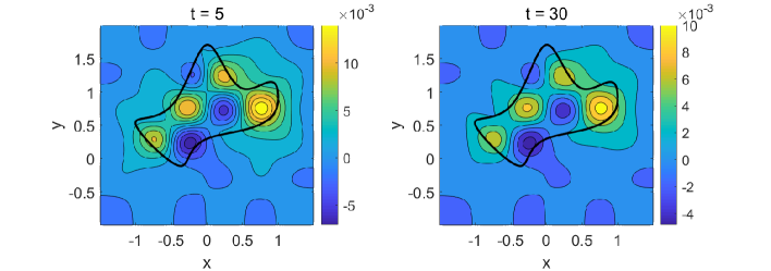
(a) $\alpha=\beta=0.2$.

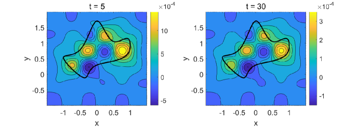
(b) $\alpha=\beta=0.8$.

Figure 18: Numerical solutions for Example 4.2, Case II, $\mu=1,\nu=10$.

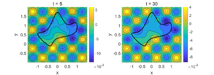
(a) $\alpha=\beta=0.2$.

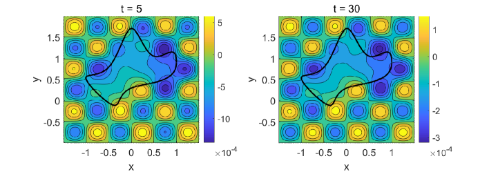
(b) $\alpha=\beta=0.8$.

Figure 19: Numerical solutions for Example 4.2, Case II, $\mu=10,\nu=1$.

5 Conclusion and discussion

We have proposed the regularized LSC method and LSFVM for solving nonlinear time-dependent PDE systems with reaction terms. In the LS method, no grid generalization is required, which makes for straightforward implementation of LS techniques. The present method can be directly extended to three-dimensional problems and can deal with moving boundary conditions at low cost, since the mass and stiffness matrices ($\mathbf{A}_{in}$ and $\mathbf{S}_{in}$ in (15), respectively) do not need to be recomputed entirely with a change of boundary. That is, we just need to add or delete some rows and columns of these matrices when the boundary changes. Extensions to three-dimensional problems and problems with moving boundary conditions will be studied in future work.

The use of the regularization reduces the condition number of the LS method, but it is still somewhat large, especially when solving the normal equation (see (31)) to obtain the numerical solutions. Fortunately, some methods have been proposed to solve ill-conditioned linear systems accurately; see [26, 27, 24, 25]. An alternative approach is solve the equivalent first-order system of (1), for which the conditioning is approximately the square root of the normal equations. This approach will be explored further in our future work, drawing on the related works in [37, 38, 39, 16]. In this work, we have considered only the use of tensor product Hermite cubic spline basis functions. In the future work, we will employ other basis functions, such as the tensor product B-spline basis functions [41]. We will also consider the local refinement to resolve the corner singularity of the solution [41].

References

- [1] T. Belytschko, Y. Krongauz, D. Organ, M. Fleming, P. Krysl, Meshless methods: An overview and recent developments, Comput. Methods Appl. Mech. Engrg. 139 (1) (1996) 3–47.
- [2] G. Liu, Y. Gu, An Introduction to Meshfree Methods and Their Programming, Springer Netherlands, 2005.
- [3] V. P. Nguyen, T. Rabczuk, S. Bordas, M. Duflot, Meshless methods: A review and computer implementation aspects, Math. Comput. Simulat. 79 (3) (2008) 763–813.
- [4] E. Carr, P. Perr , I. Turner, The extended distributed microstructure model for gradient-driven transport: A two-scale model for bypassing effective parameters, J. Comput. Phys. 327 (2016) 810–829.
- [5] I. Turner, M. Ilic, P. Perré, Modelling non-Fickian behavior in the cell walls of wood using a fractional-in-space diffusion equation, Drying Technology 29 (2011) 1932–1940.
- [6] P. Bochev, M. Gunzburger, Finite element methods of least-squares type, SIAM Review 40 (4) (1998) 789–837.
- [7] H. Ding, C. Shu, K. Yeo, D. Xu, Simulation of incompressible viscous flows past a circular cylinder by hybrid FD scheme and meshless least square-based finite difference method, Comput. Methods Appl. Mech. Engrg. 193 (9) (2004) 727–744.
- [8] E. D. Eason, A review of least squares methods for solving partial differential equations, Int. J. Numer. Methods Eng. 10 (5) (1976) 1021–1046.
- [9] A. Gelb, R. Platte, W. Rosenthal, The discrete orthogonal polynomial least squares method for approximation and solving partial differential equations, Commun. Comput. Phys. 3 (3) (2008) 734–758.
- [10] B. Keith, S. Petrides, F. Fuentes, L. Demkowicz, Discrete least-squares finite element methods, Comput. Methods Appl. Mech. Engrg. 327 (2017) 226–255.
- [11] E. Larsson, V. Shcherbakov, A. Heryudono, A least squares radial basis function partition of unity method for solving PDEs, SIAM J. Sci. Comput. 39 (6) (2017) A2538–A2563.
- [12] D. Mortari, Least-squares solution of linear differential equations, Mathematics 5 (4), (2017) 48.
- [13] B.-n. Jiang, Least-squares free collocation method mesh, Int. J. Comput. Methods 2 (9) (2012) 1240031.
- [14] J. P. Laible, G. F. Pinder, Least squares collocation solution of differential equations on irregularly shaped domains using orthogonal meshes, Numer. Methods P.D.E. 5 (4) (1989) 347–361.
- [15] J. P. Laible, G. F. Pinder, Solution of the shallow water equations by least squares collocation, Water Resources Research 29 (2) (1993) 445–455.
- [16] D. G. Zeitoun, J. P. Laible, G. F. Pinder, A weighted least squares method for first-order hyperbolic systems, Int. J. Numer. Methods Fluids 20 (1995) 191–212.
- [17] G. Golub, P. Hansen, D. O’Leary, Tikhonov regularization and total least squares, SIAM J. Matrix Anal. Appl. 21 (1) (1999) 185–194.
- [18] J. Nocedal, S. Wright, Numerical Optimization (2nd edition), Springer Science+Business Media, LLC., 2006.
- [19] B. H. Foy, P. Perré, I. Turner, The meshfree finite volume method with application to multi-phase porous media models, J. Comput. Phys. 333 (2017) 369–386.
- [20] F. Zeng, I. Turner, K. Burrage, G. E. Karniadakis, A new class of semi-implicit methods with linear complexity for nonlinear fractional differential equations, SIAM J. Sci. Comput. 40 (2018) A2986–A3011.
- [21] K. Höllig, U. Reif, J. Wipper, Weighted extended B-spline approximation of Dirichlet problems, SIAM J. Numer. Anal. 39 (2) (2001) 442–462.
- [22] W. Sun, Spectral analysis of Hermite cubic spline collocation systems, SIAM J. Numer. Anal. 36 (6) (1999) 1962–1975.
- [23] C. Van Loan, On the method of weighting for equality-constrained least-squares problems, SIAM J. Numer. Anal. 22 (5) (1985) 851–864.
- [24] A. Neumaier, Solving ill-conditioned and singular linear systems: A tutorial on regularization, SIAM Review 40 (3) (1998) 636–666.
- [25] J. Scott, M. Tuma, Solving mixed sparse-dense linear least-squares problems by preconditioned iterative methods, SIAM J. Sci. Comput. 39 (6) (2017) A2422–A2437.
- [26] E. Carson, N. J. Higham, A new analysis of iterative refinement and its application to accurate solution of ill-conditioned sparse linear systems, SIAM J. Sci. Comput. 39 (6) (2017) A2834–A2856.
- [27] L. Eldén, V. Simoncini, Solving ill-posed linear systems with GMRES and a singular preconditioner, SIAM J. Matrix Anal. Appl. 33 (4) (2012) 1369–1394.
- [28] L. D. Lorenzis, J. Evans, T. Hughes, A. Reali, Isogeometric collocation: Neumann boundary conditions and contact, Comput. Methods Appl. Mech. Engrg. 284 (2015) 21–54.
- [29] K. Diethelm, The analysis of fractional differential equations, Vol. 2004 of Lecture Notes in Mathematics, Springer-Verlag, Berlin, 2010, an application-oriented exposition using differential operators of Caputo type.
- [30] N. J. Ford, M. L. Morgado, M. Rebelo, Nonpolynomial collocation approximation of solutions to fractional differential equations, Fract. Calc. Appl. Anal. 16 (4) (2013) 874–891.
- [31] Y. Luchko, Initial-boundary problems for the generalized multi-term time-fractional diffusion equation, J. Math. Anal. Appl. 374 (2) (2011) 538–548.
- [32] I. Podlubny, Fractional differential equations, Academic Press, Inc., San Diego, CA, 1999.
- [33] K. Burrage, P. Burrage, I. Turner, F. Zeng, On the analysis of mixed-index time fractional differential equation systems, Axioms 2018 7(2) 25.
- [34] K. Diethelm, J. M. Ford, N. J. Ford, M. Weilbeer, Pitfalls in fast numerical solvers for fractional differential equations, J. Comput. Appl. Math. 186 (2) (2006) 482–503.
- [35] C. Lubich, Discretized fractional calculus, SIAM J. Math. Anal. 17 (3) (1986) 704–719.
- [36] F. Zeng, Z. Zhang, G. E. Karniadakis, Second-order numerical methods for multi-term fractional differential equations: Smooth and non-smooth solutions, Comput. Methods Appl. Mech. Engrg. 327 (1) (2017) 478–502.
- [37] Z. Cai, R. Lazarov, T. A. Manteuffel, S. F. McCormick, First-order system least squares for second-order partial differential equations: Part I, SIAM J. Numer. Anal. 31 (6) (1994) 1785–1799.
- [38] Z. Cai, T. A. Manteuffel, S. F. McCormick, First-order system least squares for second-order partial differential equations: Part II, SIAM J. Numer. Anal. 34 (2) (1997) 425–454.
- [39] N. Rekatsinas, R. Stevenson, An optimal adaptive wavelet method for first order system least squares, Numer. Math. 140 (1) (2018) 191–237.
- [40] J.F. Grcar, Optimal sensitivity analysis of linear least squares, Lawrence Berkeley National Laboratory, Report LBNL-52434, 2003.
- [41] T. J. R. Hughes, J. A. Cottrell, Y. Bazilevs, Isogeometric analysis: CAD, finite elements, NURBS, exact geometry and mesh refinement, Comput. Methods Appl. Mech. Engrg. 194 (2005) 4135–4195.