Abstract

We propose a method of using a Weighted second-order cone programming twin support vector machine (WSOCP-TWSVM) for imbalanced data classification. This method constructs a graph based under-sampling method which is utilized to remove outliers and reduce the dispensable majority samples. Then, appropriate weights are set in order to decrease the impact of samples of the majority class and increase the effect of the minority class in the optimization formula of the classifier. These weights are embedded in the optimization problem of the Second Order Cone Programming (SOCP) Twin Support Vector Machine formulations. This method is tested, and its performance is compared to previous methods on standard datasets. Results of experiments confirm the feasibility and efficiency of the proposed method.

1 Introduction

The imbalanced problem for classification methods is the basic issue of research in data mining. Datasets are said to be imbalanced if the samples belonging to majority class outnumbers the data samples belonging to the minority class. Many attempts have been made to deal with this problem in various context, such as credit scoring [Brown and Mues, 2012], fraud detection [Phua et al., 2010], spam filtering [Tang et al., 2006] and anomaly detection [Pichara and Soto, 2011]. When the training dataset is imbalanced, the difference between the performance of the majority class and minority class becomes larger. To solve this problem, two methods have been proposed: one is based on the sampling method and the other one is a cost-sensitive method. Sampling method can be divided into two classes: under-sampling method and over-sampling method. In the under-sampling, the training dataset is reduced in the majority training set so this this dataset is balanced samples of the majority sets. In the over-sampling method, data from the minority class are copied multiple times or slightly changed such that the two classes are balanced. Many issues have been made in this context, such as Random under-sampling, Random over-sampling [Kotsiantis et al., 2006], SMOTE [Bowyer et al., 2011], MSMOTE [Phua et al., 2010], Random Walk over-sampling [Zhang and Li, 2014]. An hybrid method that selects features in high dimensional datasets has also been proposed by Moradkhani et al. [2015]. Recently Ataeian et al. [2019] investigated a method for large margin classifiers.

The second approach to the imbalanced data classification problem is to apply the weights of the training data points [Elkan, 2001, Zadrozny et al., , Zhou and Liu, 2006]. Twin SVM is one of the extensions of SVM which constructing two classifiers in such a way that each one is close to one of the two classes. Note that for the imbalanced problem, the standard SVM has been modified by many researchers [Suykens et al., 2002, Deng, 2012, Tomar et al., 2014, Shao et al., 2014]. The Second-Order Cone Programming (SOCP) formulations have been proposed for SVM and Twin SVM. These formulations consider all possible choices of class-conditional densities in a way that with a given mean and covariance matrix and also with having two constraints, one for each class results in a much more efficient training [Nath and Bhattacharyya, 2007, Maldonado et al., 2016]. SOCP-TWSVM constructs two nonparallel classifiers in a way that each hyperplane is closer to one of the training patterns and at the same time as far as possible from the other. Each training pattern is represented by an ellipsoid characterized by the mean and covariance of each class.

In this paper, we attempt to extend the SOCP-TWSVM of imbalanced datasets. The proposed Weighted SOCP-TWSVM (WSOCP-TWSVM) has two phases. Firstly, it utilizes a graph-based under-sampling method to remove outliers and reduce the dispensable majority samples. Then, a weighted bias is introduced to decrease the impact of samples of the majority class and increase the effect of minority class in the optimization formula of the classifier. The SOCP is utilized to solve the model. The methods Twin-SVM, SOCP-TWSVM for binary classification are introduced in Section 2. The proposed approach is discussed in Section 3. The Experimental results are given in Section 4. The main conclusions and future works have also been provided in Section 5.

2 Preliminaries

2.1 Twin SVM

Twin SVM [Jayadeva et al., 2007] is a classification method which separates the instances by constructing two nonparallel hyperplanes instead of a hyperplane. The hyperplanes are obtained by solving two small size optimization problem using QPP. The parameters of the hyperplanes are calculated by solving the following optimization problems:

$$\begin{matrix}\begin{matrix}min\\ W_{1},b_{1},\xi_{2}\end{matrix}&\frac{1}{2}||AW_{1}+e_{1}b_{1}||^{2}+\frac{c_{1}}{2}(||W_{1}||^{2}+b_{1}^{2})+c_{3}e_{2}^{T}\xi_{2}\\ &\\ subject\leavevmode\nobreak\ to&-(BW_{1}+e_{2}b_{1})\geq e_{2}-\xi_{2},\quad\xi_{2}\geq 0,\end{matrix}$$ (1)

$$\begin{matrix}\begin{matrix}min\\ W_{2},b_{2},\xi_{1}\end{matrix}&\frac{1}{2}||BW_{2}+e_{2}b_{2}||^{2}+\frac{c_{2}}{2}(||W_{2}||^{2}+b_{2}^{2})+c_{4}e_{1}^{T}\xi_{1}\\ &\\ subject\leavevmode\nobreak\ to&-(AW_{2}+e_{1}b_{2})\geq e_{1}-\xi_{1},\quad\xi_{1}\geq 0,\end{matrix}$$ (2)

where $c_{1},c_{2},c_{3},c_{4}$ are positive parameters, and $e_{1}$ and $e_{2}$ are vectors of one of appropriates dimensions. Parameters $c_{3}$ and $c_{4}$ determine the trade-off between the respective model fit and the summation of the slack variables.

2.2 SOCP-TWSVM

This classifier has combined the ideas of Twin SVM and SOCP-SVM. The reasoning behind this approach is developing two nonparallel classifiers in a way that each hyperplane is closest to one of the two classes and also in the same distance from the other class, [Maldonado et al., 2016]. This problem can be formulated as the following quadratic programming model

$$\begin{matrix}\begin{matrix}min\\ W_{1},b_{1}\end{matrix}&\frac{1}{2}||AW_{1}+e_{1}b_{1}||^{2}+\frac{\theta_{1}}{2}(||W_{1}||^{2}+b_{1}^{2})\\ &\\ subject\leavevmode\nobreak\ to&-(W_{1}^{T}\mu_{2}-b_{1})\geq 1+\kappa_{2}||S_{2}^{T}W_{1}||,\end{matrix}$$ (3)

$$\begin{matrix}\begin{matrix}min\\ W_{2},b_{2}\end{matrix}&\frac{1}{2}||BW_{2}+e_{2}b_{2}||^{2}+\frac{\theta_{2}}{2}(||W_{2}||^{2}+b_{2}^{2})\\ &\\ subject\leavevmode\nobreak\ to&-(W_{2}^{T}\mu_{1}-b_{2})\geq 1+\kappa_{1}||S_{1}^{T}W_{2}||,\end{matrix}$$ (4)

where $\theta_{1},\theta_{2}>0$, $\Sigma_{i}=S_{i}S_{i}^{T}$ and $\Sigma_{i}$ is covariance of each class, and $\kappa_{i}=\sqrt{\frac{\eta_{i}}{1-\eta_{i}}}$ which defined as probability of false- negative (false-positive) errors.

3 WSOCP-TWSVM: Weighted SOCP-TWSVM

In this section, we present the proposed Weighted Second-Order Cone Programming Twin Support Vector Machine (WSOCP-TWSVM) for the imbalanced problem. This classifier removes outliers and reduces the unessential majority samples with a graph-based under-sampling method. Also, a weighted bias is presented to control the impact of the samples of each class. These weights define the sensitivity of the classifiers to the imbalance ratio and are considered in the mathematical model of the classifier.

3.1 Sampling method

In this method, supposing that the samples of minority class remain unchanged, and the samples of majority class are selected by constructing a proximity graph [Belkin et al., 2006, Yang et al., 2009]. The samples with nonzero degree are in high density regions; and the samples with zero degree such as outliers are in low density regions. The adjacent matrix, $U$, is defined as follows,

$$U_{ij}=\left\{\begin{array}[]{rl}\tau_{ij},&\qquad x_{i}\in N_{k}(j)\quad and\quad x_{j}\in N_{k}(i)\\ 0&\qquad otherwise\\ \end{array}\right.$$ (5)

where $(N_{k}(j))$ is a set of the k-nearest neighbors in the majority class of the point $x_{j}$, $(N_{k}(j))$ k-nearest neighbors of the point $x_{i}$, and $U$ is adjacent matrix. $\tau_{ij}$ is a a scalar value or any characters for showing k-neareast neighbors in a special vertex. $\tau_{ij}$ can be assumed any amount expect zero, and $i,j=1,..,n$. Then we define the under-sampling coefficient as

$$u_{i}=\left\{\begin{array}[]{rl}1,&\qquad\sum_{j}U_{ij}\geq k\\ 0&\qquad otherwise\\ \end{array}\right.$$ (6)

where all points with nonzero $u_{i}$ are selected as members of the sample set, Fig. 1.

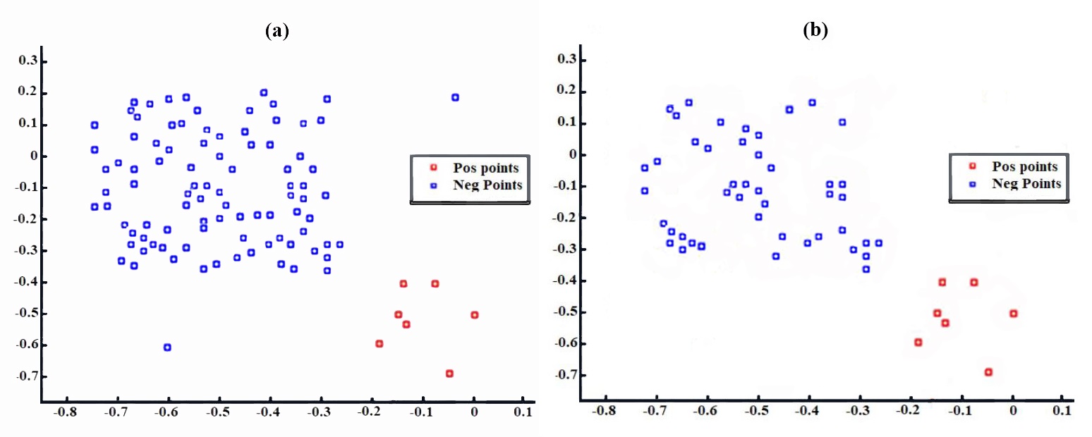
Figure 1: Decreasing the number of majority class, (a) before sampling, (b) after sampling.

3.2 Defining bias weights

In imbalanced problems, setting of the appropriate weights to the samples of training set is a critical issue in cost-sensitive approaches. The data in the majority class have to receive lower weight than those in the minority class. Also, the weight should be in (0,1) state. If the size of positive class is $N_{pos}$ and that of negative set after undersampling is $N_{-neg}$, the weights are defined as

$$D_{1}=\left\{\begin{array}[]{rl}1&\qquad N_{pos}\geq N_{-neg}\\ \frac{N_{-neg}}{N_{pos}}&\qquad N_{pos}<N_{-neg}\\ \end{array}\right.$$ (7)

$$D_{2}=\left\{\begin{array}[]{rl}\frac{N_{-neg}}{N_{pos}}&\qquad N_{pos}\geq N_{-neg}\\ 1&\qquad N_{pos}<N_{-neg}\\ \end{array}\right.$$ (8)

where $N_{-neg}$ and $N_{pos}$ are the size of negative and positive classes after sampling.

3.3 Linear Weighted SOCP twin SVM

WSOCP-TWSVM combines the graph-based under-sampling and the previous weighting methods. First, performing the under-sampling method described in Subsection 3.1, discards instances from the majority class and the remaining is demonstrated by $B_{\_}$. Then, the weight of the two classes will be calculated using Eq. (7) and Eq. (8). The majority and minority hyperplanes are determined by solving the following optimization equations

$$\begin{matrix}\begin{matrix}min\\ W_{1},b_{1},\xi_{2}\end{matrix}&\frac{1}{2}||AW_{1}+e_{1}b_{1}||^{2}+\frac{\theta_{1}}{2}(||W_{1}||^{2}+b_{1}^{2})+c_{1}D_{1}\xi_{2}\\ &\\ subject\leavevmode\nobreak\ to&-(W_{1}^{T}\mu_{2}-b_{1})\geq 1-\xi_{2}+\kappa_{2}||S_{2}^{T}W_{1}||.\xi_{2}\geq 0,\end{matrix}$$ (9)

$$\begin{matrix}\begin{matrix}min\\ W_{2},b_{2},\xi_{1}\end{matrix}&\frac{1}{2}||B_{\_}W_{2}+e_{2}b_{2}||^{2}+\frac{\theta_{2}}{2}(||W_{2}||^{2}+b_{2}^{2})+c_{2}D_{2}\xi_{1}\\ &\\ subject\leavevmode\nobreak\ to&-(W_{2}^{T}\mu_{1}-b_{2})\geq 1-\xi_{1}+\kappa_{1}||S_{1}^{T}W_{2}||.\xi_{1}\geq 0,\end{matrix}$$ (10)

where $\theta_{1},\theta_{2},c_{1},c_{2}>0,\Sigma_{2-}=S_{2-}S^{T}_{2-}$, and $\xi_{i}$ are defined as slack variables- soft margin error of the $i-th$ training point, $\mu_{i}$ is mean of each class.

Lagrangian function under Karush-Kuhn-Tucker condition and associated with Eqs. (9) and (10) can also be rewritten as

$$\hat{\mathscr{L}}(W_{1},b_{1},\lambda_{1},\rho_{1},\xi_{2},u_{2})=\frac{1}{2}||AW_{1}+e_{1}b_{1}||^{2}+\frac{\theta_{1}}{2}(||W_{1}||^{2}+b_{1}^{2})+\\ c_{1}D_{1}\xi_{2}=\lambda_{1}(W_{1}^{T}\mu_{2-}+b_{1}+1-\xi_{2}+\kappa_{2}W_{1}^{T}S_{2-}u_{2})-\rho_{1}\xi_{2}$$ (11)

$$\hat{\mathscr{L}}(W_{2},b_{2},\lambda_{2},\rho_{2},\xi_{1},u_{1})=\frac{1}{2}||BW_{2}+e_{2}b_{2}||^{2}+\frac{\theta_{1}}{2}(||W_{1}||^{2}+b_{1}^{2})+\\ c_{2}D_{2}\xi_{1}=\lambda_{2}(-W_{2}^{T}\mu_{1}+b_{2}+1-\xi_{1}+\kappa_{2}W_{2}^{T}S_{1}u_{1})-\rho_{2}\xi_{1}$$ (12)

Consequently, the dual problem can be stated as follows;

$$\ \begin{matrix}\begin{matrix}max\\ z_{1},u_{2},\lambda_{1}\end{matrix}&\frac{1}{2}\lambda_{1}^{2}Z_{1}^{T}(H^{T}H+\theta_{1}I)^{-1}Z_{1}+\lambda_{1}\\ &\\ subject\leavevmode\nobreak\ to&z_{1}=\mu_{2-}+\kappa_{2}S_{2-}u_{2},||u_{2}||\leq 1,\qquad 0\leq\lambda_{1}\leq c_{1}D_{1},\end{matrix}$$ (13)

$$\ \begin{matrix}\begin{matrix}max\\ z_{2},u_{1},\lambda_{2}\end{matrix}&\frac{1}{2}\lambda_{2}^{2}Z_{2}^{T}(G^{T}G+\theta_{2}I)^{-1}Z_{2}+\lambda_{2}\\ &\\ subject\leavevmode\nobreak\ to&z_{2}=\mu_{1}+\kappa_{1}S_{1}u_{1},||u_{1}||\leq 1,\qquad 0\leq\lambda_{2}\leq c_{2}D_{2},\end{matrix}$$ (14)

where, $H=[A,e_{1}{1}]\in R^{m*(k+1)}$, $G=[B_{\_},e_{2}]\in R^{N_{-neg}{*(k+1)}}$, $Z_{1}=[z_{1}^{T},1]^{T}\in R^{(k+1)}$, $Z_{2}=[-z_{2}^{T},-1]^{T}\in R^{(k+1)}$, $z_{1}=\mu_{2-}+\kappa_{2}S_{2-}u_{2}$, $z_{1}=\mu_{1}+\kappa_{1}S_{1}u_{1}$, and $||V||$ is equal to $sup_{||u||\leq 1}u^{T}V$.

So, Fig. (2) shows the geometrical interpolation of SOCP-TWSVM and WSOCP-TWSVM in a two-dimensional dataset. The blue points are negative samples and yellow points are removed samples in under-sampling method. The red points are positive samples. The dashed lines represent the hyperplanes constructed with SOCP-TWSVM. Similarly, the dot-dash lines correspond to the hyperplanes defined by WSOCP-TWSVM. Both methods construct a decision rule that classifies all training points correctly for the dataset. Although, the decision rules are slightly different. The method has the advantage that it optimizes both twin hyperplanes in the same optimization problem, leading to better predictive performance.

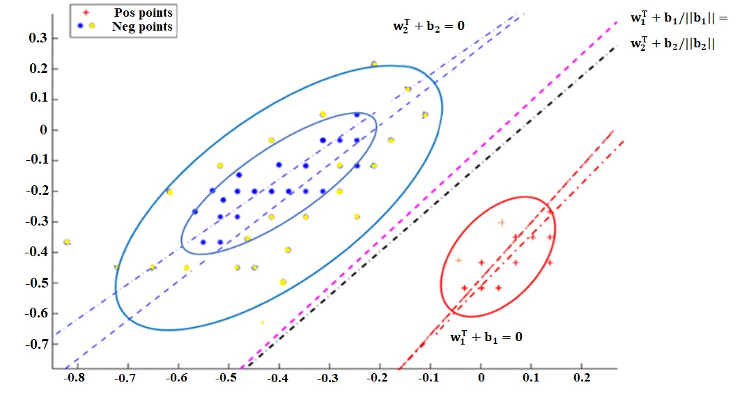
Figure 2: Geometrical interpolation of SOCP-TWSVM and WSOCP-TWSVM.

3.4 Nonlinear Weighted SOCP twin support vector machine

A kernel-based version can be derived from Eqs. (3) and (4) by rewriting weight vector $W\in R^{k}$ as $W=Xs+Mr$ where $M$ is a matrix whose columns are orthogonal to training data points. $S$ and $r$ are vectors of combining coefficients with the appropriate dimension. $X=[A^{T},B_{\_}^{T}]\in R^{k*(m+N_{-neg})}$ is the data matrix containing both training patterns. So Kernel-based Twin SOCP-SVM formulation can be written as

$$\begin{matrix}\begin{matrix}min\\ s_{1},b_{1},\xi_{2}\end{matrix}&\frac{1}{2}||K_{1}\bullet s_{1}+e_{1}b_{1}||^{2}+\frac{\theta_{1}}{2}(||s_{1}||^{2}+b_{1}^{2})+c_{1}D_{1}\xi_{2}\\ &\\ subject\leavevmode\nobreak\ to&-s_{1}^{T}g_{2}-b_{1}\geq 1-\xi_{2}+\kappa_{2}||\Lambda_{2}^{T}s_{1}||.\xi_{2}\end{matrix}$$ (15)

$$\begin{matrix}\begin{matrix}min\\ s_{2},b_{2},\xi_{1}\end{matrix}&\frac{1}{2}||K_{2}\bullet s_{2}+e_{2}b_{2}||^{2}+\frac{\theta_{2}}{2}(||s_{2}||^{2}+b_{2}^{2})+c_{2}D_{2}\xi_{1}\\ &\\ subject\leavevmode\nobreak\ to&s_{2}^{T}g_{1}+b_{2}\geq 1-\xi_{1}+\kappa_{1}||\Lambda_{1}^{T}s_{2}||.\xi_{1}\end{matrix}$$ (16)

where using a kernel function, $\Xi_{i}=\Lambda_{i}\Lambda_{i}^{T}$ for $i=1,2$, $g_{i}=\frac{1}{m_{1}}\begin{bmatrix}K_{1i}e_{i}\\ K_{2i}e_{i}\end{bmatrix}$ [Nath and Bhattacharyya, 2007, Maldonado et al., 2016].

4 Experimental Results

To show the effectiveness of the proposed WSOCP-TWSVM, we compare it with WSVM, OverSVM, UnderSVM, SMOTESVM, TWSVM and SOCP-TWSVM on 11 standard benchmark datasets from the UCI repository (https://archive.ics.uci.edu/ml/index.php). All methods are implemented in MATLAB R2014a environment.

4.1 Evaluation Criteria

The performance of different classifiers is evaluated using confusion matrix. This paper evaluates the performance of proposed methodology for class imbalance using accuracy and AUC. Accuracy of a classifier is estimated by the correct prediction made by the classifier in proportion to total number of prediction. Sensitivity of a classifier is evaluated by the percentage of positive values that are recognized accurately and also known as true positive rate. Specificity of a classifier is estimated by the percentage of negative values that are recognized correctly by the classifier. It is also known as true negative rate. Generally, the G-mean [Bowyer et al., 2011] can characterize trade-off between sensitivity and specificity. In our experiments, we also use two common performance measures associated with classifier.

4.2 Description of datasets and validation procedure

These benchmark datasets represent a wide range of fields, size and imbalanced ratios. Table 1 gives the characteristics of these datasets and minority class for each dataset is shown in the table. The rest of data are classified as the majority one. A grid search is also performed to study the influence of the parameters $\eta$ and $k$ in $KNN$ method for the new approach. In this case, we studied all combinations of the following data, $\eta_{1}={0.2,0.4,0.6,0.8}$ and $\eta_{2}={0.2,0.4,0.6,0.8}$, where $\eta_{1}$ and $\eta_{2}$ are the maximum false positive and false negative error, respectively. The K parameter is selected from the set $\{3,5,10,15\}$, and all other parameters for WSVM, TWSVM, SOCP-TWSVM and our WSOCP-TWSVM is selected from the set $\{10^{-9},...,10^{-6}\}$, also we consider $c_{1}=c_{2}$ and $c_{3}=c_{4}$. For the above procedure, we employ libsvm [Chang and Lin, 2011] to be the base classifier of SVM and the SeDuMi MATLAB toolbox as the SOCP-based classifiers [Sturm, 1999].

4.3 Test using UCI database

We study the following classification approaches; the Weighted SVM, OverSVM, UnderSVM, SMOTESVM, TWSVM, and SOCP-TWSVM, and WSOCP-TWSVM. For each dataset, seven different classifiers were trained and tested by using nested $10$ cross-validation technique. The accuracy and G-mean of this cross-validation process are averaged for ten runs. The average accuracy of the compared classifiers with linear kernel and the nonlinear kernel is summarized in Tables 2 and 4. It can be concluded that WSOCP-TWSVM has best performance in compared with SOCP-TWSVM in most cases. For instance, WSOCP-TWSVM in Yeast3 and Heberman datasets is better than other classifiers. Generally, the methods like TWSVM and oversampling have better result for datasets with great imbalanced ratio like PimaIndian and Ionosphere. Our results on big datasets like Pageblocks infer that that WSOCP-TWSVM possesses a better accuracy in compared with other classifiers. Average G-mean of the compared classifiers with linear kernel and the nonlinear kernel is summarized in Tables 3 and 5 which indicates the excellence of the performance of WSOCP-TWSVM in compared with SOCP-TWSVM. Tables 6 and 7 show the training time for these seven classifiers with linear and nonlinear kernel. The algorithm’s execution time naturally increased by running the sampling phase at the beginning of the run. Regarding the execution time in both kernel states, it can be concluded that the sampling phase has a higher overhead time rather than other methods. In particular, SOCPTWSVM rather than the other classifiers possess the highest execution time for some databases like German and Yeast3. In general, the runtime in the WSOCP-TWSVM algorithm is greater than the SOCPTWSVM method but the accuracy of the new method is higher.

The Friedman test [Friedman, 1939] is a non-parametric statistical test that is used to detect differences in treatments across multiple test attempts by considering their ranking. This test is employed here to detect differences by our method. The Friedman test confirms that our strategy is better than other comparable methods in terms of accuracy. For linear cases, the result of the Friedman test is presented in Table 8 (a) and (b) and for nonlinear cases, the result of the test is presented in Table 8 (c) and (d). The ranking results from the Friedman test show that WSOCP-TWSVM performs better than other methods. Based on results, for linear cases, though the accuracy of the WSOCP-TWSVM is similar to that of SMOTESVM, the accuracy of WSVM is a little worse than both. Also, the G-mean of WSOCP-TWSVM and SMOTESVM are similar and both have the best performance. The results on nonlinear classifiers have shown that accuracy of the SMOTESVM is a little worse than our WSOCP-TWSVM, the G-mean of SOCP-TWSVM is lower than WSOCP-TWSVM. We can see that our proposed approach obtains the best-imbalanced classification performance than the others in most cases, specifically, it enhances the performance of SOCP-TWSVM.

5 Conclusion

A new method of imbalanced data classification named WSOCP-TWSVM is proposed in the present paper. This method uses the under-sampling procedure for training the dataset and gives the weights for each class. The results of numerical tests performed on datasets show that the proposed methodology is feasible and effective on generalization ability. The WSOCP-TWSVM method is better than the others in the kernel case. Introducing this method provides opportunities to continue the future works. Our method can be extended to multi-class classifications and used for some practical application. In addition, the employment of some different weight setting methods can improve the performance of the WSOCP-TWSVM method.

Table 1: Characteristics of the benchmark datasets.

Dataset	IR	#Features	Minority class	Data size
Yeast3	0.1098	8	ME3	1484
Vehicle	0.2362	18	VAN	946
Transfusion	0.2380	4	Yes	748
Wine	0.3315	13	Class 1	178
PimaIndian	0.3490	8	Diabetes	768
Ionosphere	0.3590	34	Bad	351
Haberman	0.2647	3	Died	306
German	0.3000	20	Bad	1000
CMC	0.2261	9	Lon-term	1473
Yeast4	0.0340	8	ME2	1484
Wisconsin	0.1021	9	Rest	683
Segment	0.1427	19	Segment	2308
Page-blocks	0.1021	10	Rest	5472

Table 2: The training accuracy of linear classifiers on benchmark datasets

Dataset	WSVM	OverSVM	UnderSVM	SMOTESVM	TWSVM	SOCP-TWSVM	WSOCP-TWSVM
Yeast3	90.79$\pm$1.36	90.22$\pm$0.15	83.78$\pm$0.19	91.92$\pm$0.39	89.17$\pm$0.41	90.56$\pm$3.05	92.35$\pm$3.25
Vehicle	95.80$\pm$0.86	94.67$\pm$0.10	93.83$\pm$0.85	97.03$\pm$0.24	96.59$\pm$0.23	95.65$\pm$3.98	94.23$\pm$1.04
Transfusion	62.73$\pm$4.28	54.86$\pm$2.21	55.69$\pm$2.67	65.06$\pm$3.73	49.43$\pm$2.27	59.45$\pm$4.26	65.23$\pm$8.79
Wine	92.12$\pm$0.50	95.72$\pm$0.55	91.20$\pm$0.73	96.04$\pm$0.19	94.81$\pm$0.50	93.38$\pm$10.10	92.92$\pm$7.03
PimaIndian	75.64$\pm$0.79	75.26$\pm$0.90	72.79$\pm$0.53	73.01$\pm$0.62	76.10$\pm$0.25	71.23$\pm$7.83	74.42$\pm$0.36
Ionosphere	88.75$\pm$2.29	89.11$\pm$0.67	83.62$\pm$0.44	73.01$\pm$0.30	84.93$\pm$1.21	83.73$\pm$4.52	84.90$\pm$3.27
Haberman	70.68$\pm$0.92	64.82$\pm$0.51	58.96$\pm$1.74	74.77$\pm$0.28	75.81$\pm$0.46	75.89$\pm$6.67	76.53$\pm$6.72
German	72.30$\pm$1.28	71.68$\pm$1.58	49.99$\pm$0.47	69.66$\pm$0.63	74.84$\pm$0.30	73.70$\pm$3.12	72.90$\pm$6.15
CMC	73.46$\pm$0.35	71.25$\pm$0.17	51.94$\pm$0.78	75.83$\pm$0.41	74.36$\pm$0.21	76.64$\pm$1.17	77.39$\pm$0.26
Yeast4	94.29$\pm$0.25	84.98$\pm$0.18	87.06$\pm$1.73	96.50$\pm$0.26	75.10$\pm$0.16	90.89$\pm$2.37	92.12$\pm$2.07
Wisconsin	96.72$\pm$0.73	93.37$\pm$0.26	93.10$\pm$0.24	95.92$\pm$0.17	95.34$\pm$0.25	94.13$\pm$2.75	94.02$\pm$9.35
Segment	92.26$\pm$0.21	92.52$\pm$0.42	91.26$\pm$0.87	90.24$\pm$0.32	91.26$\pm$0.25	95.24$\pm$0.58	93.16$\pm$0.45
Page-blocks	90.87$\pm$0.25	91.24$\pm$2.03	87.15$\pm$0.13	90.15$\pm$0.45	92.54$\pm$0.16	92.14$\pm$0.18	92.54$\pm$0.36

Table 3: The training G-mean of linear classifiers on benchmark datasets.

Dataset	WSVM	OverSVM	UnderSVM	SMOTESVM	TWSVM	SOCP-TWSVM	WSOCP-TWSVM
Yeast3	78.02$\pm$1.20	76.23$\pm$0.15	71.75$\pm$1.69	84.93$\pm$0.73	83.07$\pm$0.96	91.48$\pm$4.85	93.23$\pm$3.16
Vehicle	90.38$\pm$0.74	91.69$\pm$0.41	86.91$\pm$0.80	96.05$\pm$0.27	93.74$\pm$0.43	89.17$\pm$3.26	90.33$\pm$1.62
Transfusion	58.68$\pm$2.75	61.31$\pm$2.72	56.97$\pm$2.66	62.06$\pm$3.18	52.72$\pm$0.36	56.82$\pm$4.26	63.24$\pm$3.02
Wine	76.57$\pm$1.64	82.07$\pm$2.56	80.20$\pm$2.73	84.72$\pm$2.19	86.87$\pm$1.36	88.02$\pm$8.66	90.52$\pm$0.52
PimaIndian	66.39$\pm$2.16	71.24$\pm$0.92	68.79$\pm$0.53	72.01$\pm$1.51	70.43$\pm$2.80	63.75$\pm$3.25	71.52$\pm$8.03
Ionosphere	75.59$\pm$1.26	80.54$\pm$0.44	62.09$\pm$0.41	77.31$\pm$0.93	75.67$\pm$0.97	76.47$\pm$8.73	79.49$\pm$3.82
Haberman	60.84$\pm$2.85	62.90$\pm$0.67	52.15$\pm$3.48	66.92$\pm$0.50	52.21$\pm$4.90	52.73$\pm$11.51	58.96$\pm$4.24
German	59.09$\pm$3.62	67.09$\pm$3.50	61.96$\pm$3.37	64.24$\pm$1.83	65.47$\pm$2.51	71.95$\pm$4.71	70.03$\pm$5014
CMC	52.91$\pm$1.08	50.58$\pm$2.17	45.56$\pm$1.29	60.43$\pm$1.76	54.61$\pm$2.22	59.83$\pm$5.22	64.91$\pm$5.28
Yeast4	73.48$\pm$2.01	82.02$\pm$0.19	67.93$\pm$1.97	84.35$\pm$0.18	18.78$\pm$6.20	80.93$\pm$6.79	85.36$\pm$8.85
Wisconsin	96.49$\pm$0.36	91.40$\pm$0.21	89.14$\pm$0.24	93.54$\pm$0.18	92.04$\pm$0.52	90.71$\pm$5.72	89.86$\pm$7.07
Segment	94.12$\pm$0.34	90.45$\pm$0.15	84.26$\pm$0.95	75.15$\pm$0.12	90.15$\pm$0.89	95.14$\pm$0.23	94.15$\pm$0.85
Page-blocks	75.25$\pm$0.23	85.12$\pm$0.31	70.12$\pm$0.16	85.12$\pm$0.45	85.12$\pm$0.13	90.25$\pm$0.12	91.25$\pm$0.23

Table 4: The training accuracy of nonlinear classifiers on benchmark datasets.

Dataset	WSVM	OverSVM	UnderSVM	SMOTESVM	TWSVM	SOCPTWSV	WSOCP-TWSVM
Yeast3	91.39$\pm$1.77	92.91$\pm$1.04	87.61$\pm$3.42	93.52$\pm$1.49	92.31$\pm$0.16	91.91$\pm$2.01	92.31$\pm$0.78
Vehicle	78.54$\pm$0.89	80.60$\pm$1.89	74.16$\pm$2.56	82.80$\pm$1.52	79.47$\pm$1.65	94.10$\pm$4.32	93.89$\pm$2.43
Transfusio	73.25$\pm$2.35	74.85$\pm$1.38	68.59$\pm$1.17	75.60$\pm$2.59	60.16$\pm$3.29	77.14$\pm$4.76	72.31$\pm$3.51
Wine	84.28$\pm$2.18	95.73$\pm$3.48	77.62$\pm$1.17	92.51$\pm$2.64	92.15$\pm$2.07	92.16$\pm$5.70	92.19$\pm$3.67
PimaIndia	62.79$\pm$1.61	65.10$\pm$0.37	64.42$\pm$2.28	73.42$\pm$1.78	72.23$\pm$1.72	73.43$\pm$3.24	73.53$\pm$4.69
Ionosphere	93.67$\pm$1.59	91.63$\pm$2.64	87.45$\pm$2.36	94.32$\pm$1.71	90.30$\pm$0.47	92.90$\pm$3.26	90.31$\pm$5.35
Haberman	73.55$\pm$3.14	74.24$\pm$1.15	58.96$\pm$2.68	72.77$\pm$2.41	69.39$\pm$1.56	75.83$\pm$6.28	76.03$\pm$5.33
German	71.24$\pm$3.01	68.45$\pm$0.39	60.43$\pm$1.58	71.53$\pm$0.29	70.47$\pm$1.86	70.00$\pm$3.43	72.50$\pm$4.37
CMC	62.25$\pm$2.07	68.13$\pm$1.65	60.27$\pm$1.89	71.74$\pm$2.20	73.62$\pm$1.55	78.34$\pm$2.34	78.12$\pm$7.14
Yeast4	92.63$\pm$1.39	94.07$\pm$2.86	92.49$\pm$1.73	95.48$\pm$1.82	92.16$\pm$2.79	94.55$\pm$0.20	95.67$\pm$3.02
Wisconsin	93.65$\pm$2.25	94.26$\pm$0.86	91.28$\pm$2.58	96.16$\pm$0.81	96.02$\pm$0.72	95.85$\pm$1.70	96.56$\pm$2.28
Segment	78.15$\pm$0.25	89.15$\pm$0.45	65.14$\pm$0.45	62.24$\pm$0.15	89.12$\pm$0.14	90.15$\pm$2.13	89.84$\pm$2.03
Page-blocks	90.15$\pm$0.23	89.14$\pm$2.01	85.16$\pm$0.45	89.15$\pm$1.02	89.14$\pm$0.17	90.01$\pm$2.01	90.05$\pm$0.30

Table 5: The training G-mean of nonlinear classifiers on benchmark datasets.

Dataset	WSVM	OverSVM	UnderSVM	SMOTESVM	TWSVM	SOCP-TWSVM	WSOCP-TWSVM
Yeast3	81.05$\pm$1.46	80.73$\pm$0.45	74.14$\pm$1.25	85.32$\pm$0.83	78.68$\pm$2.57	91.99$\pm$2.01	91.60$\pm$3.37
Vehicle	81.05$\pm$1.39	84.31$\pm$0.42	69.41$\pm$2.44	90.61$\pm$1.29	63.08$\pm$3.30	90.56$\pm$7.26	91.99$\pm$4.56
Transfusio	57.55$\pm$1.83	50.89$\pm$2.89	43.97$\pm$1.50	60.52$\pm$2.04	51.90$\pm$1.21	61.21$\pm$6.99	63.96$\pm$5.14
Wine	7.52$\pm$18.94	71.93$\pm$4.62	0.00$\pm$0.00	67.44$\pm$2.81	60.87$\pm$2.68	91.73$\pm$5.75	92.39$\pm$7.57
PimaIndia	48.63$\pm$2.73	54.89$\pm$3.11	19.74$\pm$8.51	58.42$\pm$3.20	57.16$\pm$2.68	70.54$\pm$3.31	71.04$\pm$4.12
Ionosphere	93.93$\pm$1.60	94.07$\pm$2.56	72.44$\pm$2.96	93.35$\pm$2.95	90.73$\pm$3.14	93.67$\pm$3.13	93.84$\pm$8.11
Haberman	35.52$\pm$1.47	43.78$\pm$11.1	29.26$\pm$2.18	51.61$\pm$1.58	41.37$\pm$2.36	60.77$\pm$10.24	63.00$\pm$10.53
German	59.25$\pm$0.73	58.79$\pm$1.31	0.00$\pm$0.00	65.12$\pm$0.47	54.12$\pm$3.25	59.74$\pm$7.17	65.23$\pm$7.33
CMC	64.04$\pm$7.38	62.23$\pm$2.98	54.34$\pm$2.00	41.05$\pm$5.40	53.64$\pm$2.19	66.18$\pm$3.91	66.41$\pm$5.19
Yeast4	31.13$\pm$3.01	51.24$\pm$1.05	40.17$\pm$4.15	48.08$\pm$1.63	46.66$\pm$2.54	60.36$\pm$8.91	62.64$\pm$10.21
Wisconsin	75.98$\pm$0.53	84.26$\pm$8.29	90.48$\pm$2.51	94.44$\pm$1.32	93.85$\pm$3.20	95.22$\pm$2.04	96.85$\pm$1.90
Segment	59.15$\pm$0.23	60.15$\pm$0.58	65.15$\pm$0.26	62.23$\pm$0.68	80.95$\pm$2.01	90.26$\pm$0.12	89.12$\pm$3.01
Page-blocks	76.25$\pm$2.09	85.12$\pm$0.10	90.12$\pm$0.85	91.25$\pm$2.05	94.15$\pm$0.10	93.12$\pm$0.15	94.16$\pm$0.32

Table 6: The training time of linear classifiers on benchmark datasets.

Dataset	WSVM	OverSVM	UnderSVM	SMOTESVM	TWSVM	SOCP-TWSVM	WSOCP-TWSVM
Yeast3	0.3925	0.1389	0.0523	0.0255	0.9262	0.6223	0.8526
Vehicle	0.5615	2.1526	0.8342	0.9523	1.8954	0.4562	0.9856
Transfusio	38.9526	46.2535	16.2589	26.4590	0.8962	0.4895	68.2568
Wine	0.9523	0.3214	0.2561	0.4151	0.0059	0.1452	0.6231
PimaIndia	2.0311	8.1645	2.0030	6.0310	0.0215	0.0279	0.08536
Ionosphere	0.0521	0.0295	0.0152	0.2560	0.0310	0.2613	0.0361
Haberman	0.1652	0.1025	0.0214	0.1389	0.0321	0.2140	0.6231
German	29.4510	35.1500	15.2301	23.1547	0.8925	0.5216	0.6954
CMC	3.2514	1.3259	15.1614	16.2400	0.7316	1.1632	2.0311
Yeast4	0.2798	0.1624	0.0921	0.1232	0.1456	0.1315	0.4510
Wisconsin	0.2151	0.1361	0.9526	0.2920	0.0258	0.3621	0.8925
Segment	1.2561	0.8745	0.9325	0.6214	0.6258	0.7546	0.9847
Page-blocks	94.1561	195.1232	39.1621	354.1212	45.6251	23.1514	38.7916

Table 7: The training time of nonlinear classifiers on benchmark datasets.

Dataset	WSVM	OverSVM	UnderSVM	SMOTESVM	TWSVM	SOCP-TWSVM	WSOCP-TWSVM
Yeast3	0.5961 0.1988	0.0958	0.1523	0.0981	0.02359	0.1650
Vehicle	0.8945	0.3012	0.0952	0.2135	0.6254	0.4512	0.6895
Transfusio	0.6250	0.1523	0.0258	0.0987	0.0984	0.9890	1.0230
Wine	0.0231	0.1325	0.0102	0.0189	0.0236	0.0166	0.3250
PimaIndia	0.0625	0.0562	0.0154	0.0231	0.1541	0.0950	0.1621
Ionosphere	0.0352	0.2315	0.0165	0.0152	0.0925	0.0239	0.1451
Haberman	0.0451	0.1298	0.1451	0.1241	0.1648	0.0252	0.2145
German	3.0261	3.1203	3.1285	0.0231	0.2378	0.0234	0.2611
CMC	2.3714	0.2315	0.1458	0.1485	0.1547	0.1898	0.5210
Yeast4	0.2154	0.0591	0.0721	0.0915	0.1524	0.0699	0.5921
Wisconsin	0.1584	0.7925	0.7891	0.0214	0.0599	0.9851	1.2561
Segment	1.8548	0.9550	0.0214	0.0528	0.0951	0.9512	1.0320
Page-blocks	31.0252	7.8912	0.98521	6.2511	46.0259	21.0985	36.0695

Table 8: Friedman test rank of accuracy and G-mean of linear and nonlinear classifiers. (a) acc-lin (b) G-mean-lin (c)acc-non-lin (d) G-mean-nonlin.

	Mean rank		Mean rank		Mean rank		Mean rank
WSVM	4.73	WSVM	3.18	WSVM	3.00	WSVM	3.09
OverSVM	3.36	OverSVM	4.45	OverSVM	4.18	OverSVM	3.82
UnderSVM	1.55	UnderSVM	1.64	UnderSVM	1.27	UnderSVM	1.55
SMOTESVM	4.91	SMOTESVM	5.64	SMOTESVM	5.55	SMOTESVM	4.45
TWSVM	4.36	TWSVM	3.55	TWSVM	3.14	TWSVM	2.64
SOCP-TWSVM	4.18	SOCP-TWSVM	3.91	SOCP-TWSVM	5.18	SOCP-TWSVM	5.73
WSOCP-TWSVM	4.93	WSOCP-TWSVM	5.66	WSOCP-TWSVM	5.68	WSOCP-TWSVM	6.98
(a)		(b)		(c)		(d)

References

- Ataeian et al. [2019] Hassan Ataeian, Shahriar Esmaeili, Ali Amiri, Neda Maleki Khas, and Hossein Safari. Qlmc-hd: Quasi large margin classifier based on hyperdisk. arXiv preprint arXiv:1902.09692, 2019.
- Belkin et al. [2006] Mikhail Belkin, Partha Niyogi, and Vikas Sindhwani. Manifold regularization: A geometric framework for learning from labeled and unlabeled examples. J. Mach. Learn. Res., 7:2399–2434, December 2006. ISSN 1532-4435. URL http://dl.acm.org/citation.cfm?id=1248547.1248632.
- Bowyer et al. [2011] Kevin W. Bowyer, Nitesh V. Chawla, Lawrence O. Hall, and W. Philip Kegelmeyer. SMOTE: synthetic minority over-sampling technique. CoRR, abs/1106.1813, 2011. URL http://arxiv.org/abs/1106.1813.
- Brown and Mues [2012] Iain Brown and Christophe Mues. An experimental comparison of classification algorithms for imbalanced credit scoring data sets. Expert Systems with Applications, 39(3):3446–3453, feb 2012. doi: 10.1016/j.eswa.2011.09.033. URL https://doi.org/10.1016%2Fj.eswa.2011.09.033.
- Chang and Lin [2011] Chih-Chung Chang and Chih-Jen Lin. Libsvm: A library for support vector machines. ACM Trans. Intell. Syst. Technol., 2(3):27:1–27:27, May 2011. ISSN 2157-6904. doi: 10.1145/1961189.1961199. URL http://doi.acm.org/10.1145/1961189.1961199.
- Deng [2012] Naiyang Deng. Support Vector Machines. Chapman and Hall/CRC, dec 2012. doi: 10.1201/b14297. URL https://doi.org/10.1201%2Fb14297.
- Elkan [2001] Charles Elkan. The foundations of cost-sensitive learning. In Proceedings of the 17th International Joint Conference on Artificial Intelligence - Volume 2, IJCAI’01, pages 973–978, San Francisco, CA, USA, 2001. Morgan Kaufmann Publishers Inc. ISBN 1-55860-812-5, 978-1-558-60812-2. URL http://dl.acm.org/citation.cfm?id=1642194.1642224.
- Friedman [1939] Milton Friedman. A correction: The use of ranks to avoid the assumption of normality implicit in the analysis of variance. Journal of the American Statistical Association, 34(205):109, mar 1939. doi: 10.2307/2279169. URL https://doi.org/10.2307%2F2279169.
- Jayadeva et al. [2007] Jayadeva, R. Khemchandani, and Suresh Chandra. Twin support vector machines for pattern classification. IEEE Transactions on Pattern Analysis and Machine Intelligence, 29(5):905–910, May 2007. ISSN 0162-8828. doi: 10.1109/TPAMI.2007.1068.
- Kotsiantis et al. [2006] Sotiris Kotsiantis, Dimitris Kanellopoulos, and Panayiotis Pintelas. Handling imbalanced datasets: A review, 2006.
- Maldonado et al. [2016] Sebastián Maldonado, Julio López, and Miguel Carrasco. A second-order cone programming formulation for twin support vector machines. Applied Intelligence, 45(2):265–276, feb 2016. doi: 10.1007/s10489-016-0764-4. URL https://doi.org/10.1007%2Fs10489-016-0764-4.
- Moradkhani et al. [2015] Mostafa Moradkhani, Ali Amiri, Mohsen Javaherian, and Hossein Safari. A hybrid algorithm for feature subset selection in high-dimensional datasets using FICA and IWSSr algorithm. Applied Soft Computing, 35:123–135, oct 2015. doi: 10.1016/j.asoc.2015.03.049. URL https://doi.org/10.1016%2Fj.asoc.2015.03.049.
- Nath and Bhattacharyya [2007] J. Saketha Nath and C. Bhattacharyya. Maximum margin classifiers with specified false positive and false negative error rates. In Proceedings of the 2007 SIAM International Conference on Data Mining. Society for Industrial and Applied Mathematics, apr 2007. doi: 10.1137/1.9781611972771.4. URL https://doi.org/10.1137%2F1.9781611972771.4.
- Phua et al. [2010] Clifton Phua, Vincent Lee, Kate Smith, and Ross Gayler. A comprehensive survey of data mining-based fraud detection research. 2010. doi: 10.1016/j.chb.2012.01.002.
- Pichara and Soto [2011] Karim Pichara and Alvaro Soto. Active learning and subspace clustering for anomaly detection. Intelligent Data Analysis, 15(2):151–171, mar 2011. doi: 10.3233/ida-2010-0461. URL https://doi.org/10.3233%2Fida-2010-0461.
- Shao et al. [2014] Yuan-Hai Shao, Wei-Jie Chen, Jing-Jing Zhang, Zhen Wang, and Nai-Yang Deng. An efficient weighted lagrangian twin support vector machine for imbalanced data classification. Pattern Recognition, 47(9):3158–3167, sep 2014. doi: 10.1016/j.patcog.2014.03.008. URL https://doi.org/10.1016%2Fj.patcog.2014.03.008.
- Sturm [1999] Jos F. Sturm. Using SeDuMi 1.02, a matlab toolbox for optimization over symmetric cones. Optimization Methods and Software, 11(1-4):625–653, jan 1999. doi: 10.1080/10556789908805766. URL https://doi.org/10.1080%2F10556789908805766.
- Suykens et al. [2002] J.A.K. Suykens, J. De Brabanter, L. Lukas, and J. Vandewalle. Weighted least squares support vector machines: robustness and sparse approximation. Neurocomputing, 48(1-4):85–105, oct 2002. doi: 10.1016/s0925-2312(01)00644-0. URL https://doi.org/10.1016%2Fs0925-2312%2801%2900644-0.
- Tang et al. [2006] Yuchun Tang, Sven Krasser, Paul Judge, and Yan-Qing Zhang. Fast and effective spam sender detection with granular SVM on highly imbalanced mail server behavior data. In 2006 International Conference on Collaborative Computing: Networking, Applications and Worksharing. IEEE, nov 2006. doi: 10.1109/colcom.2006.361856. URL https://doi.org/10.1109%2Fcolcom.2006.361856.
- Ting [2002] Kai Ming Ting. An instance-weighting method to induce cost-sensitive trees. IEEE Transactions on Knowledge and Data Engineering, 14(3):659–665, may 2002. doi: 10.1109/tkde.2002.1000348. URL https://doi.org/10.1109%2Ftkde.2002.1000348.
- Tomar et al. [2014] Divya Tomar, Shubham Singhal, and Sonali Agarwal. Weighted least square twin support vector machine for imbalanced dataset. International Journal of Database Theory and Application, 7(2):25–36, apr 2014. doi: 10.14257/ijdta.2014.7.2.03. URL https://doi.org/10.14257%2Fijdta.2014.7.2.03.
- Yang et al. [2009] Xubing Yang, Songcan Chen, Bin Chen, and Zhisong Pan. Proximal support vector machine using local information. Neurocomputing, 73(1-3):357–365, dec 2009. doi: 10.1016/j.neucom.2009.08.002. URL https://doi.org/10.1016%2Fj.neucom.2009.08.002.
- [23] B. Zadrozny, J. Langford, and N. Abe. Cost-sensitive learning by cost-proportionate example weighting. In Third IEEE International Conference on Data Mining. IEEE Comput. Soc. doi: 10.1109/icdm.2003.1250950. URL https://doi.org/10.1109%2Ficdm.2003.1250950.
- Zhang and Li [2014] Huaxiang Zhang and Mingfang Li. RWO-sampling: A random walk over-sampling approach to imbalanced data classification. Information Fusion, 20:99–116, nov 2014. doi: 10.1016/j.inffus.2013.12.003. URL https://doi.org/10.1016%2Fj.inffus.2013.12.003.
- Zhou and Liu [2006] Zhi-Hua Zhou and Xu-Ying Liu. Training cost-sensitive neural networks with methods addressing the class imbalance problem. IEEE Transactions on Knowledge and Data Engineering, 18(1):63–77, jan 2006. doi: 10.1109/tkde.2006.17. URL https://doi.org/10.1109%2Ftkde.2006.17.