Non-Stochastic Information Theory

Abstract

In an effort to develop the foundations for a non-stochastic theory of information, the notion of $\delta$-mutual information between uncertain variables is introduced as a generalization of Nair’s non-stochastic information functional. Several properties of this new quantity are illustrated, and used to prove a channel coding theorem in a non-stochastic setting. Namely, it is shown that the largest $\delta$-mutual information between received and transmitted codewords over $\epsilon$-noise channels equals the $(\epsilon,\delta)$-capacity. This notion of capacity generalizes the Kolmogorov $\epsilon$-capacity to packing sets of overlap at most $\delta$, and is a variation of a previous definition proposed by one of the authors. Results are then extended to more general noise models, and to non-stochastic, memoryless, stationary channels. Finally, sufficient conditions are established for the factorization of the $\delta$-mutual information and to obtain a single letter capacity expression. Compared to previous non-stochastic approaches, the presented theory admits the possibility of decoding errors as in Shannon’s probabilistic setting, while retaining a worst-case, non-stochastic character.

I Introduction

This paper introduces elements of a non-stochastic information theory that parallels Shannon’s probabilistic theory of information, but that provides strict deterministic guarantees for every codeword transmission. When Shannon laid the mathematical foundations of communication theory he embraced a probabilistic approach [1]. A tangible consequence of this choice is that in today’s communication systems performance is guaranteed in an average sense, or with high probability. Occasional violations from a specification are permitted, and cannot be avoided. This approach is well suited for consumer-oriented digital communication devices, where the occasional loss of data packets is not critical, and made Shannon’s theory the golden standard to describe communication limits, and to construct codes that achieve these limits. The probabilistic approach, however, has also prevented Shannon’s theory to be relevant in systems where occasional decoding errors can result in catastrophic failures; or in adversarial settings, where the behavior of the channel may be unknown and cannot be described by a probability distribution. The basic consideration that is the leitmotiv of this paper is that the probabilistic framework is not a fundamental component of Shannon’s theory, and that the path laid by Shannon’s work can be extended to embrace a non-stochastic setting.

The idea of adopting a non-stochastic approach in information theory is not new. A few years after introducing the notion of capacity of a communication system [1], Shannon introduced the zero-error capacity [2]. While the first notion corresponds to the largest rate of communication such that the probability of decoding error tends to zero, the second corresponds to the largest rate of communication such that the probability of decoding error equals zero. Both definitions of capacity satisfy coding theorems: Shannon’s channel coding theorem states that the capacity is the supremum of the mutual information between the input and the output of the channel [1]. Nair introduced a non-stochastic mutual information functional and established an analogous coding theorem for the zero-error capacity in a non-stochastic setting [3]. While Shannon’s theorem leads to a single letter expression, Nair’s result is multi-letter, involving the non-stochastic information between codeword blocks of $n$ symbols. The zero-error capacity can also be formulated as a graph-theoretic property and the absence of a single-letter expression for general graphs is well known [2, 4]. Extensions of Nair’s nonstochastic approach to characterize the zero-error capacity in the presence of feedback from the receiver to the transmitter using nonstochastic directed mutual information have also been considered [5].

A parallel non-stochastic approach is due to Kolmogorov who, motivated by Shannon’s results, introduced the notions of $\epsilon$-entropy and $\epsilon$-capacity in the context of functional spaces [6]. He defined the $\epsilon$-entropy as the logarithm base two of the covering number of the space, namely the logarithm of the minimum number of balls of radius $\epsilon$ that can cover the space. Determining this number is analogous to designing a source codebook such that the distance between any signal in the space and a codeword is at most $\epsilon$. In this way, any transmitted signal can be represented by a codeword point with at most $\epsilon$-distortion. Notions related to the $\epsilon$-entropy are the Hartley entropy [7] and the Rényi differential (0th-order) entropy [8]. They arise for random variables with known range but unknown distribution, and are defined by taking the logarithm of the cardinality (for discrete variables), or Lebesgue measure (for continuous variables) of their range. Thus, their definition does not require any statistical structure. Using these entropies, non-stochastic measures of mutual information have been constructed [9, 10]. Unfortunately, the absence of coding theorems makes the operational significance of these definitions lacking.

Rather than using mutual information and entropy, Kolmogorov gave an operational definition of the $\epsilon$-capacity as the logarithm base two of the packing number of the space, namely the logarithm of the maximum number of balls of radius $\epsilon$ that can be placed in the space without overlap. Determining this number is analogous to designing a channel codebook such that the distance between any two codewords is at least $2\epsilon$. In this way, any transmitted codeword that is subject to a perturbation of at most $\epsilon$ can be recovered at the receiver without error. It follows that the $\epsilon$-capacity corresponds to the zero-error capacity of an additive channel having arbitrary, bounded noise of support at most $[0,\epsilon]$. Lim and Franceschetti extended this concept introducing the $(\epsilon,\delta)$ capacity [11], defined as the logarithm base two of the largest number of balls of radius $\epsilon$ that can be placed in the space with average codeword overlap of at most $\delta$. In this setting, $\delta$ measures the amount of error that can be tolerated when designing a codebook in a non-stochastic setting. Neither the Kolmogorov capacity, nor its $(\epsilon,\delta)$ generalization have a corresponding information-theoretic characterization in terms of mutual information and an associated coding theorem. This is offered in the present paper. Some possible applications of non-stochastic approaches arising in the context of estimation, control, security, communication over non-linear optical channels, and robustness of neural networks are described in [12, 13, 14, 15, 16, 17, 18]; and some are also discussed in the context of the presented theory at the end of the paper.

The rest of the paper is organized as follows. Section II provides a summary of our contributions; Section III introduces the mathematical framework of non-stochastic uncertain variables that is used throughout the paper. Section IV introduces the concept of non-stochastic mutual information. Section V gives an operational definition of capacity of a communication channel and relates it to the mutual information. Section VI extends results to more general channel models; and section VII concentrates on the special case of stationary, memoryless, uncertain channels. Sufficient conditions are obtained to obtain single-letter expressions for this case. Section VIII considers some examples of channels and computes the corresponding capacity. Finally, Section IX discusses some possible application of the developed theory, and Section X draws conclusions and discusses future directions. A subset of the results has been presented in [19].

II Contributions

We introduce a notion of $\delta$-mutual information between non-stochastic, uncertain variables. In contrast to Nair’s definition  [3], which only allows to measure information with full confidence, our definition considers the information revealed by one variable regarding the other with a given level of confidence. We then introduce a notion of $(\epsilon,\delta)$-capacity, defined as the logarithm base two of the largest number of balls of radius $\epsilon$ that can be placed in the space such that the overlap between any two balls is at most a ratio of $\delta$ and the total number of balls. In contrast to the definition of Lim and Franceschetti [11], which requires the average overlap among all the balls to be at most $\delta$, our definition requires to bound the overlap between any pair of balls. For $\delta=0$, our capacity definition reduces to the Kolmogorov $\epsilon$-capacity, or equivalently to the zero-error capacity of an additive, bounded noise channel, and our mutual information definition reduces to Nair’s one [3]. We establish a channel coding theorem in this non-stochastic setting, showing that the largest mutual information, with confidence at least $(1-\delta)$, between a transmitted codeword and its received version corrupted with noise at most $\epsilon$, is the $(\epsilon,\delta)$-capacity. We then extend this result to more general non-stochastic channels, where the noise is expressed in terms of a set-valued map $N(\cdot)$ associating each transmitted codeword to a noise region in the received codeword space, that is not necessarily a ball of radius $\epsilon$.

Next, we consider the class of non-stochastic, memoryless, stationary uncertain channels. In this case, the noise $N(\cdot)$ experienced by a codeword of $n$ symbols factorizes into $n$ identical terms describing the noise experienced by each codeword symbol. This is the non-stochastic analogous of a discrete memoryless channel (DMC), where the current output symbol depends only on the current input symbol and not on any of the previous input symbols, and the noise distribution is constant across symbol transmissions. It differs from Kolmogorov’s $\epsilon$-noise channel, where the noise experienced by one symbol affects the noise experienced by other symbols. In Kolmogorov’s setting, the noise occurs within a ball of radius $\epsilon$. It follows that for any realization where the noise along one dimension (viz. symbol) is close to $\epsilon$, the noise experienced by all other symbols lying in the remaining dimensions must be close to zero. In contrast, for non-stochastic, memoryless, stationary channels, the noise experienced by any transmitted symbol is described by a single, non-stochastic set-value map from the transmitted alphabet to the received symbol space. We provide coding theorems in this setting in terms of the $\delta$-mutual information rate between received and transmitted codewords. Finally, we provide sufficient conditions for the factorization of the mutual information and to obtain a single-letter expression for the non-stochastic capacity of stationary, memoryless, uncertain channels. We provide examples in which these conditions are satisfied and compute the corresponding capacity, and we conclude with a discussion of some possible applications of the presented theory.

III Uncertain variables

We start by reviewing the mathematical framework used in [3] to describe non-stochastic uncertain variables (UVs). An UV $X$ is a mapping from a sample space $\Omega$ to a set $\mathscr{X}$, i.e. for all $\omega\in\Omega$, we have $x=X(\omega)\in\mathscr{X}$. Given an UV $X$, the marginal range of $X$ is

$$\llbracket X\rrbracket=\{X(\omega):\omega\in\Omega\}.$$ (1)

The joint range of two UVs $X$ and $Y$ is

$$\llbracket X,Y\rrbracket=\{(X(\omega),Y(\omega)):\omega\in\Omega\}.$$ (2)

Given an UV $Y$, the conditional range of $X$ given $Y=y$ is

$$\llbracket X|y\rrbracket=\{X(\omega):Y(\omega)=y,\omega\in\Omega\},$$ (3)

and the conditional range of $X$ given $Y$ is

$$\llbracket X|Y\rrbracket=\{\llbracket X|y\rrbracket:y\in\llbracket Y\rrbracket\}.$$ (4)

Thus, $\llbracket X|Y\rrbracket$ denotes the uncertainty in $X$ given the realization of $Y$ and $\llbracket X,Y\rrbracket$ represents the total joint uncertainty of $X$ and $Y$, namely

$$\llbracket X,Y\rrbracket=\cup_{y\in\llbracket Y\rrbracket}\llbracket X|y\rrbracket\times\{y\}.$$ (5)

Finally, two UVs $X$ and $Y$ are independent if for all $x\in\llbracket X\rrbracket$

$$\llbracket Y|x\rrbracket=\llbracket Y\rrbracket,$$ (6)

which also implies that for all $y\in\llbracket Y\rrbracket$

$$\llbracket X|y\rrbracket=\llbracket X\rrbracket.$$ (7)

IV $\delta$-Mutual information

IV-A Uncertainty function

We now introduce a class of functions that are used to express the amount of uncertainty in determining one UV given another. In our setting, an uncertainty function associates a positive number to a given set, which expresses the “massiveness” or “size” of that set.

Definition 1.

Given any set $\mathscr{X}$, $m_{\mathscr{X}}:\mathscr{S}\subseteq\mathscr{X}\to\mathbb{R}_{0}^{+}$ is an uncertainty function if it is finite and strongly transitive, namely:

For all $\mathscr{S}\subseteq\mathscr{X},\mathscr{S}\not=\emptyset,$ we have

$$0<m_{\mathscr{X}}(\mathscr{S})<\infty,\;m_{\mathscr{X}}(\emptyset)=0.$$ (8)

For all $\mathscr{S}_{1},\mathscr{S}_{2}\subseteq\mathscr{X},$ we have

$$\max\{m_{\mathscr{X}}(\mathscr{S}_{1}),m_{\mathscr{X}}(\mathscr{S}_{2})\}\leq m_{\mathscr{X}}(\mathscr{S}_{1}\cup\mathscr{S}_{2}).$$ (9)

In the case $\mathscr{X}$ is measurable, an uncertainty function can easily be constructed using a measure. In the case $\mathscr{X}$ is a bounded (not necessarily measurable) metric space and the input set $\mathscr{S}$ contains at least two points, an example of uncertainty function is the diameter.

IV-B Association and dissociation between UVs

We now introduce notions of association and dissociation between UVs. In the following definitions, we let $m_{\mathscr{X}}(.)$ and $m_{\mathscr{Y}}(.)$ be uncertainity functions defined over sets $\mathscr{X}$ and $\mathscr{Y}$ corresponding to UVs $X$ and $Y$. We use the notation $\mathscr{A}\succ\delta$ to indicate that for all $a\in\mathscr{A}$ we have $a>\delta$. Similarly, we use $\mathscr{A}\preceq\delta$ to indicate that for all $a\in\mathscr{A}$ we have $a\leq\delta$. For $\mathscr{A}=\emptyset$, we assume $\mathscr{A}\preceq\delta$ is always satisfied, while $\mathscr{A}\succ\delta$ is not. Whenever we consider $i\not=j$, we also assume that $y_{i}\not=y_{j}$ and $x_{i}\not=x_{j}$.

Definition 2.

The sets of association for UVs $X$ and $Y$ are

$$\mathscr{A}(X;Y) =\bigg{\{}\frac{m_{\mathscr{X}}(\llbracket X|y_{1}\rrbracket\cap\llbracket X|y_{2}\rrbracket|)}{m_{\mathscr{X}}(\llbracket X\rrbracket)}:y_{1},y_{2}\in\llbracket Y\rrbracket\bigg{\}}\setminus\big{\{}0\big{\}},$$ (10)

$$\mathscr{A}(Y;X) =\bigg{\{}\frac{m_{\mathscr{Y}}(\llbracket Y|x_{1}\rrbracket\cap\llbracket Y|x_{2}\rrbracket|)}{m_{\mathscr{Y}}(\llbracket Y\rrbracket)}:\;x_{1},x_{2}\in\llbracket X\rrbracket\bigg{\}}\setminus\big{\{}0\big{\}}.$$ (11)

Definition 3.

For any $\delta_{1},\delta_{2}\in[0,1)$, UVs $X$ and $Y$ are disassociated at levels $(\delta_{1},\delta_{2})$ if the following inequalities hold:

$$\mathscr{A}(X;Y)\succ\delta_{1},$$ (12)

$$\mathscr{A}(Y;X)\succ\delta_{2},$$ (13)

and this case we write $(X,Y)\stackrel{{\scriptstyle d}}{{\leftrightarrow}}(\delta_{1},\delta_{2})$.

Having UVs $X$ and $Y$ be disassociated at levels $(\delta_{1},\delta_{2})$ indicates that at least two conditional ranges $\llbracket X|y_{1}\rrbracket$ and $\llbracket X|y_{2}\rrbracket$ have nonzero overlap, and that given any two conditional ranges, either they do not overlap or the uncertainty associated to their overlap is greater than a $\delta_{1}$ fraction of the total uncertainty associated to $\llbracket X\rrbracket$; and that the same holds for conditional ranges $\llbracket Y|x_{1}\rrbracket$ and $\llbracket Y|x_{2}\rrbracket$ and level $\delta_{2}$. The levels of disassociation can be viewed as lower bounds on the amount of residual uncertainty in each variable when the other is known. If $X$ and $Y$ are independent, then all the conditional ranges completely overlap, $\mathscr{A}(X;Y)$ and $\mathscr{A}(Y;X)$ contain only the element one, and the variables are maximally disassociated (see Figure 1a).

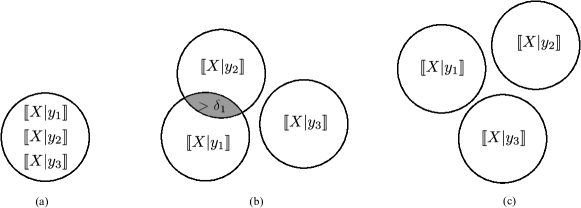
Figure 1: Illustration of disassociation between UVs. Case (a): variables are maximally disassociated and all conditional ranges completely overlap. Case (b): variables are disassociated at some levels $(\delta_{1},\delta_{2})$, and there is some overlap between at least two conditional ranges. Case (c): variables are not disassociated at any levels, and there is no overlap between the conditional ranges.

In this case, knowledge of $Y$ does not reduce the uncertainty of $X$, and vice versa. On the other hand, when the uncertainty associated to any of the non-zero intersections of the conditional ranges decreases, but remains positive, then $X$ and $Y$ become less disassociated, in the sense that knowledge of $Y$ can reduce the residual uncertainty of $X$, and vice versa (see Figure 1b). When the intersection between every pair of conditional ranges becomes empty, the variables cease being disassociated (see Figure 1c).

An analogous definition of association is given to provide upper bounds on the residual uncertainty of one uncertain variable when the other is known.

Definition 4.

For any $\delta_{1},\delta_{2}\in[0,1]$, we say that UVs $X$ and $Y$ are associated at levels $(\delta_{1},\delta_{2})$ if the following inequalities hold:

$$\mathscr{A}(X;Y)\preceq\delta_{1},$$ (14)

$$\mathscr{A}(Y;X)\preceq\delta_{2},$$ (15)

and in this case we write $(X,Y)\stackrel{{\scriptstyle a}}{{\leftrightarrow}}(\delta_{1},\delta_{2})$.

The following lemma provides necessary and sufficient conditions for association at given levels to hold. These conditions are stated for all points in the marginal ranges $\llbracket Y\rrbracket$ and $\llbracket X\rrbracket$. They show that in the case of association one can also include in the definition the conditional ranges that have zero intersection. This is not the case for disassociation.

Lemma 1.

For any $\delta_{1},\delta_{2}\in[0,1]$, $(X,Y)\stackrel{{\scriptstyle a}}{{\leftrightarrow}}(\delta_{1},\delta_{2})$ if and only if for all $y_{1},y_{2}\in\llbracket Y\rrbracket$, we have

$$\frac{m_{\mathscr{X}}(\llbracket X|y_{1}\rrbracket\cap\llbracket X|y_{2}\rrbracket|)}{m_{\mathscr{X}}(\llbracket X\rrbracket)}\leq\delta_{1},$$ (16)

and for all $x_{1},x_{2}\in\llbracket X\rrbracket$, we have

$$\frac{m_{\mathscr{Y}}(\llbracket Y|x_{1}\rrbracket\cap\llbracket Y|x_{2}\rrbracket|)}{m_{\mathscr{Y}}(\llbracket Y\rrbracket)}\leq\delta_{2}.$$ (17)

Proof.

The proof is given in Appendix -A. ∎

An immediate, yet important consequence of our definitions is that both association and disassociation at given levels $(\delta_{1},\delta_{2})$ cannot hold simultaneously. We also have that, given any two UVs, one can always choose $\delta_{1}$ and $\delta_{2}$ to be large enough such that they are associated at levels $(\delta_{1},\delta_{2})$. In contrast, as the smallest value in the sets $\mathcal{A}(X;Y)$ and $\mathcal{A}(Y;X)$ tends to zero, the variables eventually cease being disassociated. Finally, it is possible that two uncertain variables are neither associated nor disassociated at given levels $(\delta_{1},\delta_{2})$.

Example 1.

Consider three individuals $a$, $b$ and $c$ going for a walk along a path. Assume they take at most $15$, $20$ and $10$ minutes to finish their walk, respectively. Assume $a$ starts walking at time 5:00, $b$ starts walking at 5:10 and $c$ starts walking at 5:20. Figure 2

Figure 2: Illustration of the possible time intervals for the walkers on the path.

shows the possible time intervals for the walkers on the path. Let an uncertain variable $W$ represent the set of walkers that are present on the path at any time, and an uncertain variable $T$ represent the time at which any walker on the path finishes its walk. Then, we have the marginal ranges

$$\llbracket W\rrbracket=\{\{a\},\{b\},\{c\},\{a,b\},\{b,c\}\},$$ (18)

$$\llbracket T\rrbracket=[\mbox{5:00},\mbox{5:30}].$$ (19)

We also have the conditional ranges

$$\llbracket T|\{a\}\rrbracket=[\mbox{5:00},\mbox{5:15}],$$ (20)

$$\llbracket T|\{b\}\rrbracket=[\mbox{5:10},\mbox{5:30}],$$ (21)

$$\llbracket T|\{c\}\rrbracket=[\mbox{5:20},\mbox{5:30}],$$ (22)

$$\llbracket T|\{a,b\}\rrbracket=[\mbox{5:10},\mbox{5:15}],$$ (23)

$$\llbracket T|\{b,c\}\rrbracket=[\mbox{5:20},\mbox{5:30}].$$ (24)

For all $t\in[\mbox{5:00},\mbox{5:10})$, we have

$$\llbracket W|t\rrbracket=\{\{a\}\},$$ (25)

for all $t\in[\mbox{5:10},\mbox{5:15}]$, we have

$$\llbracket W|t\rrbracket=\{\{a,b\},\{a\},\{b\}\},$$ (26)

for all $t\in(\mbox{5:15},\mbox{5:20})$, we have

$$\llbracket W|t\rrbracket=\{\{b\}\},$$ (27)

and for all $t\in[\mbox{5:20},\mbox{5:30}]$, we have

$$\llbracket W|t\rrbracket=\{\{b,c\},\{b\},\{c\}\}.$$ (28)

Now, let the uncertainty function of a time set $\mathscr{S}$ be

$$m_{\mathscr{T}}(\mathscr{S})=\begin{cases}\mathcal{L}(\mathscr{S})+10\mbox{ if }\mathscr{S}\neq\emptyset,\\ 0\mbox{ otherwise },\end{cases}$$ (29)

where $\mathcal{L}(\cdot)$ is the Lebesgue measure. Let the uncertainty function $m_{\mathscr{W}}(.)$ associated to a set of individuals be the cardinality of the set. Then, the sets of association are

$$\mathscr{A}(W;T)=\{1/5,3/5\},$$ (30)

$$\mathscr{A}(T;W)=\{3/8,1/2\}.$$ (31)

It follows that that for all $\delta_{1}<1/5$ and $\delta_{2}<3/8$, we have

$$(W,T)\stackrel{{\scriptstyle d}}{{\leftrightarrow}}(\delta_{1},\delta_{2}),$$ (32)

and the residual uncertainty in $W$ given $T$ is at least $\delta_{1}$ fraction of the total uncertainty in $W$, while the residual uncertainty in $T$ given $W$ is at least $\delta_{2}$ fraction of the total uncertainty in $T$. On the other hand, for all $\delta_{1}\geq 3/5$ and $\delta_{2}\geq 1/2$ we have

$$(W,T)\stackrel{{\scriptstyle a}}{{\leftrightarrow}}(\delta_{1},\delta_{2}),$$ (33)

and the residual uncertainty in $W$ given $T$ is at most $\delta_{1}$ fraction of the total uncertainty in $W$, while the residual uncertainty in $T$ given $W$ is at most $\delta_{2}$ fraction of the total uncertainty in $T$.

Finally, if $1/5\leq\delta_{1}<3/5$ or $3/8\leq\delta_{2}<1/2$, then $W$ and $T$ are neither associated nor disassociated.

IV-C $\delta$-mutual information

We now introduce the mutual information between uncertain variables in terms of some structural properties of covering sets. Intuitively, for any $\delta\in[0,1]$ the $\delta$-mutual information, expressed in bits, represents the most refined knowledge that one uncertain variable provides about the other, at a given level of confidence $(1-\delta)$. We express this idea by considering the quantization of the range of uncertainty of one variable, induced by the knowledge of the other. Such quantization ensures that the variable can be identified with uncertainty at most $\delta$. The notions of association and disassociation introduced above are used to ensure that the mutual information is well defined, namely it can be positive, and enjoys a certain symmetric property.

Definition 5.

$\delta$-Connectedness and $\delta$-isolation.

• For any $\delta\in[0,1]$, points $x_{1},x_{2}\in\llbracket X\rrbracket$ are $\delta$-connected via $\llbracket X|Y\rrbracket$, and are denoted by $x_{1}\stackrel{{\scriptstyle\delta}}{{\leftrightsquigarrow}}x_{2}$, if there exists a finite sequence $\{\llbracket X|y_{i}\rrbracket\}_{i=1}^{N}$ of conditional sets such that $x_{1}\in\llbracket X|y_{1}\rrbracket$, $x_{2}\in\llbracket X|y_{N}\rrbracket$ and for all $1<i\leq N$, we have

  $$\frac{m_{\mathscr{X}}(\llbracket X|y_{i}\rrbracket\cap\llbracket X|y_{i-1}\rrbracket)}{m_{\mathscr{X}}(\llbracket X\rrbracket)}>\delta.$$ (34)

  If $x_{1}\stackrel{{\scriptstyle\delta}}{{\leftrightsquigarrow}}x_{2}$ and $N=1$, then we say that $x_{1}$ and $x_{2}$ are singly $\delta$-connected via $\llbracket X|Y\rrbracket$, i.e. there exists a $y$ such that $x_{1},x_{2}\in\llbracket X|y\rrbracket$.

• A set $\mathscr{S}\subseteq\llbracket X\rrbracket$ is (singly) $\delta$-connected via $\llbracket X|Y\rrbracket$ if every pair of points in the set is (singly) $\delta$-connected via $\llbracket X|Y\rrbracket$.

• Two sets $\mathscr{S}_{1},\mathscr{S}_{2}\subseteq\llbracket X\rrbracket$ are $\delta$-isolated via $\llbracket X|Y\rrbracket$ if no point in $\mathscr{S}_{1}$ is $\delta$-connected to any point in $\mathscr{S}_{2}$.

Definition 6.

$\delta$-overlap family.
For any $\delta\in[0,1]$, a $\llbracket X|Y\rrbracket$ $\delta$-overlap family of $\llbracket X\rrbracket$, denoted by $\llbracket X|Y\rrbracket^{*}_{\delta}$, is a largest family of distinct sets covering $\llbracket X\rrbracket$ such that:

1. Each set in the family is $\delta$-connected and contains at least one singly $\delta$-connected set of the form $\llbracket X|y\rrbracket$.

2. The measure of overlap between any two distinct sets in the family is at most $\delta m_{\mathscr{X}}(\llbracket X\rrbracket)$.

3. For every singly $\delta$-connected set, there exist a set in the family containing it.

The first property of the $\delta$-overlap family ensures that points in the same set of the family cannot be distinguished with confidence at least $(1-\delta)$, while also ensuring that each set cannot be arbitrarily small. The second and third properties ensure that points that are not covered by the same set of the family can be distinguished with confidence at least $(1-\delta)$. It follows that the cardinality of the covering family represents the most refined knowledge at a given level of confidence $(1-\delta)$ that we can have about $X$, given the knowledge of $Y$. This also corresponds to the most refined quantization of the set $\llbracket X\rrbracket$ induced by $Y$. This interpretation is analogous to the one in [3], extending the concept of overlap partition introduced there to a $\delta$-overlap family in this work. The stage is now set to introduce the $\delta$-mutual information in terms of the $\delta$-overlap family.

Definition 7.

The $\delta$-mutual information provided by $Y$ about $X$ is

$$I_{\delta}(X;Y)=\log_{2}|\llbracket X|Y\rrbracket^{*}_{\delta}|\mbox{ bits},$$ (35)

if a $\llbracket X|Y\rrbracket$ $\delta$-overlap family of $\llbracket X\rrbracket$ exists, otherwise it is zero.

We now show that when variables are associated at level $(\delta,\delta_{2})$, then there exists a $\delta$-overlap family, so that the mutual information is well defined.

Theorem 1.

If $(X,Y)\stackrel{{\scriptstyle a}}{{\leftrightarrow}}(\delta,\delta_{2})$, then there exists a $\delta$-overlap family $\llbracket X|Y\rrbracket^{*}_{\delta}$.

Proof.

We show that

$$\llbracket X|Y\rrbracket=\{\llbracket X|y\rrbracket:y\in\llbracket Y\rrbracket\}$$ (36)

is a $\delta$-overlap family. First, note that $\llbracket X|Y\rrbracket$ is a cover of $\llbracket X\rrbracket$, since $\llbracket X\rrbracket=\cup_{y\in\llbracket Y\rrbracket}\llbracket X|y\rrbracket$. Second, each set in the family $\llbracket X|Y\rrbracket$ is singly $\delta$-connected via $\llbracket X|Y\rrbracket$, since trivially any two points $x_{1},x_{2}\in\llbracket X|y\rrbracket$ are singly $\delta$-connected via the same set. It follows that Property 1 of Definition 6 holds.

Now, since $(X,Y)\stackrel{{\scriptstyle a}}{{\leftrightarrow}}(\delta,\delta_{2})$, then by Lemma 1 for all $y_{1},y_{2}\in\llbracket Y\rrbracket$ we have

$$\frac{m_{\mathscr{X}}(\llbracket X|y_{1}\rrbracket\cap\llbracket X|y_{2}\rrbracket)}{m_{\mathscr{X}}(\llbracket X\rrbracket)}\leq\delta,$$ (37)

which shows that Property 2 of Definition 6 holds. Finally, it is also easy to see that Property 3 of Definition 6 holds, since $\llbracket X|Y\rrbracket$ contains all sets $\llbracket X|y\rrbracket$. ∎

Next, we show that a $\delta$-overlap family also exists when variables are disassociated at level $(\delta,\delta_{2})$. In this case, we also characterize the mutual information in terms of a partition of $\llbracket X\rrbracket$.

Definition 8.

$\delta$-isolated partition.
A $\llbracket X|Y\rrbracket$ $\delta$-isolated partition of $\llbracket X\rrbracket$, denoted by $\llbracket X|Y\rrbracket_{\delta}$, is a partition of $\llbracket X\rrbracket$ such that any two sets in the partition are $\delta$-isolated via $\llbracket X|Y\rrbracket$.

Theorem 2.

If $(X,Y)\stackrel{{\scriptstyle d}}{{\leftrightarrow}}(\delta,\delta_{2})$, then we have:

1. There exists a unique $\delta$-overlap family $\llbracket X|Y\rrbracket^{*}_{\delta}$.

2. The $\delta$-overlap family is the $\delta$-isolated partition of largest cardinality, namely for any $\llbracket X|Y\rrbracket_{\delta}$, we have

   $$|\llbracket X|Y\rrbracket_{\delta}|\leq|\llbracket X|Y\rrbracket^{*}_{\delta}|,$$ (38)

   where the equality holds if and only if $\llbracket X|Y\rrbracket_{\delta}=\llbracket X|Y\rrbracket^{*}_{\delta}$.

Proof.

First, we show the existence of a ${\delta}$-overlap family. For all $x\in\llbracket X\rrbracket$, let $\mathscr{C}(x)$ be the set of points that are $\delta$-connected to $x$ via $\llbracket X|Y\rrbracket$, namely

$$\mathscr{C}(x)=\{x_{1}\in\llbracket X\rrbracket:x\stackrel{{\scriptstyle\delta}}{{\leftrightsquigarrow}}x_{1}\}.$$ (39)

Then, we let

$$\mathcal{C}=\{\mathscr{C}(x):x\in\llbracket X\rrbracket\},$$ (40)

and show that this is a $\delta$-overlap family. First, note that since $\llbracket X\rrbracket=\cup_{\mathscr{S}\in\mathcal{C}}\mathscr{S}$, we have that $\mathcal{C}$ is a cover of $\llbracket X\rrbracket$. Second, for all $\mathscr{C}(x)\in\mathcal{C}$ there exists a $y\in\llbracket Y\rrbracket$ such that $x\in\llbracket X|y\rrbracket$, and since any two points $x_{1},x_{2}\in\llbracket X|y\rrbracket$ are singly $\delta$-connected via $\llbracket X|Y\rrbracket$, we have that $\llbracket X|y\rrbracket\subseteq\mathscr{C}(x)$. It follows that every set in the family $\mathcal{C}$ contains at least one singly $\delta$-connected set. For all $x_{1},x_{2}\in\mathscr{C}(x)$, we also have $x_{1}\stackrel{{\scriptstyle\delta}}{{\leftrightsquigarrow}}x$ and $x\stackrel{{\scriptstyle\delta}}{{\leftrightsquigarrow}}x_{2}$. Since $(X,Y)\stackrel{{\scriptstyle d}}{{\leftrightarrow}}(\delta,\delta_{2})$, by Lemma 4 in Appendix -D this implies $x_{1}\stackrel{{\scriptstyle\delta}}{{\leftrightsquigarrow}}x_{2}$. It follows that every set in the family $\mathcal{C}$ is $\delta$-connected and contains at least one singly $\delta$-connected set, and we conclude that Property 1 of Definition 6 is satisfied.

We now claim that for all $x_{1},x_{2}\in\llbracket X\rrbracket$, if

$$\mathscr{C}(x_{1})\neq\mathscr{C}(x_{2}),$$ (41)

then

$$m_{\mathscr{X}}(\mathscr{C}(x_{1})\cap\mathscr{C}(x_{2}))=0.$$ (42)

This can be proven by contradiction. Let $\mathscr{C}(x_{1})\neq\mathscr{C}(x_{2})$ and assume that $m_{\mathscr{X}}(\mathscr{C}(x_{1})\cap\mathscr{C}(x_{2}))\neq 0$. By (8) this implies that $\mathscr{C}(x_{1})\cap\mathscr{C}(x_{2})\neq\emptyset$. We can then pick $z\in\mathscr{C}(x_{1})\cap\mathscr{C}(x_{2})$, such that we have $z\stackrel{{\scriptstyle\delta}}{{\leftrightsquigarrow}}x_{1}$ and $z\stackrel{{\scriptstyle\delta}}{{\leftrightsquigarrow}}x_{2}$. Since $(X,Y)\stackrel{{\scriptstyle d}}{{\leftrightarrow}}(\delta,\delta_{2})$, by Lemma 4 in Appendix -D this also implies $x_{1}\stackrel{{\scriptstyle\delta}}{{\leftrightsquigarrow}}x_{2}$ , and therefore $\mathscr{C}(x_{1})=\mathscr{C}(x_{2})$, which is a contradiction. It follows that if $\mathscr{C}(x_{1})\neq\mathscr{C}(x_{2})$, then we must have $m_{\mathscr{X}}(\mathscr{C}(x_{1})\cap\mathscr{C}(x_{2}))=0$, and therefore

$$\frac{m_{\mathscr{X}}(\mathscr{C}(x_{1})\cap\mathscr{C}(x_{2}))}{m_{\mathscr{X}}(\llbracket X\rrbracket)}=0\leq\delta.$$ (43)

We conclude that Property 2 of Definition 6 is satisfied.

Finally, we have that for any singly $\delta$-connected set $\llbracket X|y\rrbracket$, there exist an $x\in\llbracket X\rrbracket$ such that $x\in\llbracket X|y\rrbracket$, which by (39) implies $\llbracket X|y\rrbracket\subseteq\mathscr{C}(x)$. Namely, for every singly $\delta$-connected set, there exist a set in the family containing it. We can then conclude that $\mathcal{C}$ satisfies all the properties of a $\delta$-overlap family.

Next, we show that $\mathcal{C}$ is a unique $\delta$-overlap family. By contradiction, consider another $\delta$-overlap family $\mathcal{D}$. For all $x\in\llbracket X\rrbracket$, let $\mathscr{D}(x)$ denote a set in $\mathcal{D}$ containing $x$. Then, using the definition of $\mathscr{C}(x)$ and the fact that $\mathscr{D}(x)$ is $\delta$-connected, it follows that

$$\mathscr{D}(x)\subseteq\mathscr{C}(x).$$ (44)

Next, we show that for all $x\in\llbracket X\rrbracket$, we also have

$$\mathscr{C}(x)\subseteq\mathscr{D}(x),$$ (45)

from which we conclude that $\mathcal{D}=\mathcal{C}$.

The proof of (45) is also obtained by contradiction. Assume there exists a point $\tilde{x}\in\mathscr{C}(x)\setminus\mathscr{D}(x)$. Since both $x$ and $\tilde{x}$ are contained in $\mathscr{C}(x)$, we have $\tilde{x}\stackrel{{\scriptstyle\delta}}{{\leftrightsquigarrow}}x$. Let $x^{*}$ be a point in a singly-connected set that is contained in $\mathscr{D}(x)$, namely $x^{*}\in\llbracket X|y^{*}\rrbracket\subseteq\mathscr{D}(x)$. Since both $x$ and $x^{*}$ are in $\mathscr{D}(x)$, we have that $x\stackrel{{\scriptstyle\delta}}{{\leftrightsquigarrow}}x^{*}$. Since $(X,Y)\stackrel{{\scriptstyle d}}{{\leftrightarrow}}(\delta,\delta_{2})$, we can apply Lemma 4 in Appendix -D to conclude that $\tilde{x}\stackrel{{\scriptstyle\delta}}{{\leftrightsquigarrow}}x^{*}$. It follows that there exists a sequence of conditional ranges $\{\llbracket X|y_{i}\rrbracket\}_{i=1}^{N}$ such that $\tilde{x}\in\llbracket X|y_{1}\rrbracket$ and $x^{*}\in\llbracket X|y_{N}\rrbracket$, which satisfies (34). Since $x^{*}$ is in both $\llbracket X|y_{N}\rrbracket$ and $\llbracket X|y^{*}\rrbracket$, we have $\llbracket X|y_{N}\rrbracket\cap\llbracket X|y^{*}\rrbracket\not=\emptyset$ and since $(X,Y)\stackrel{{\scriptstyle d}}{{\leftrightarrow}}(\delta,\delta_{2})$, we have

$$\frac{m_{\mathscr{X}}(\llbracket X|y_{N}\rrbracket\cap\llbracket X|y^{*}\rrbracket)}{m_{\mathscr{X}}(\llbracket X\rrbracket)}>\delta.$$ (46)

Without loss of generality, we can then assume that the last element of our sequence is $\llbracket X|y^{*}\rrbracket$. By Property 3 of Definition 6, every conditional range in the sequence must be contained in some set of the $\delta$-overlap family $\mathcal{D}$. Since $\llbracket X|y^{*}\rrbracket\subseteq\mathscr{D}(x)$ and $\llbracket X|y_{1}\rrbracket\not\subseteq\mathscr{D}(x)$, it follows that there exist two consecutive conditional ranges along the sequence and two sets of the $\delta$-overlap family covering them, such that $\llbracket X|y_{i-1}\rrbracket\subseteq\mathscr{D}(x_{i-1})$, $\llbracket X|y_{i}\rrbracket\subseteq\mathscr{D}(x_{i})$, and $\mathscr{D}(x_{i-1})\not=\mathscr{D}(x_{i})$. Then, we have

$$\begin{split}&\;m_{\mathscr{X}}(\mathscr{D}(x_{i-1})\cap\mathscr{D}(x_{i}))\\ =&\;m_{\mathscr{X}}((\llbracket X|y_{i-1}\rrbracket\cap\llbracket X|y_{i}\rrbracket)\cup(\mathscr{D}(x^{*}_{i-1})\cap\mathscr{D}(x^{*}_{i})))\\ \stackrel{{\scriptstyle(a)}}{{\geq}}&\;m_{\mathscr{X}}(\llbracket X|y_{i-1}\rrbracket\cap\llbracket X|y_{i}\rrbracket)\\ \stackrel{{\scriptstyle(b)}}{{>}}&\;\delta m_{\mathscr{X}}(\llbracket X\rrbracket),\end{split}$$ (47)

where $(a)$ follows from (9) and $(b)$ follows from (34). It follows that

$$\frac{m_{\mathscr{X}}(\mathscr{D}(x_{i-1})\cap\mathscr{D}({x_{i}}))}{m_{\mathscr{X}}(\llbracket X\rrbracket)}>\delta,$$ (48)

and Property 2 of Definition 6 is violated. Thus, $\tilde{x}$ does not exists, which implies $\mathscr{C}(x)\subseteq\mathscr{D}(x)$. Combining (44) and (45), we conclude that the $\delta$-overlap family $\mathcal{C}$ is unique.

We now turn to the proof of the second part of the Theorem. Since by (43) the uncertainty associated to the overlap between any two sets of the $\delta$-overlap family $\mathcal{C}$ is zero, it follows that $\mathcal{C}$ is also a partition.

Now, we show that $\mathcal{C}$ is also a $\delta$-isolated partition. This can be proven by contradiction. Assume $\mathcal{C}$ is not a $\delta$-isolated partition. Then, there exists two distinct sets $\mathscr{C}(x_{1}),\mathscr{C}(x_{2})\in\mathcal{C}$ such that $\mathscr{C}(x_{1})$ and $\mathscr{C}(x_{2})$ are not $\delta$-isolated. This implies that there exists a point $\bar{x}_{1}\in\mathscr{C}(x_{1})$ and $\bar{x}_{2}\in\mathscr{C}(x_{2})$ such that $\bar{x}_{1}\stackrel{{\scriptstyle\delta}}{{\leftrightsquigarrow}}\bar{x}_{2}$. Using the fact that $\mathscr{C}(x_{1})$ and $\mathscr{C}(x_{2})$ are $\delta$-connected and Lemma 4 in Appendix -D, this implies that all points in the set $\mathscr{C}(x_{1})$ are $\delta$-connected to all points in the set $\mathscr{C}(x_{2})$. Now, let $x_{1}^{*}$ and $x_{2}^{*}$ be points in a singly $\delta$-connected set contained in $\mathscr{C}(x_{1})$ and $\mathscr{C}(x_{2})$ respectively, namely $x^{*}_{1}\in\llbracket X|y^{*}_{1}\rrbracket\subseteq\mathscr{C}(x_{1})$ and $x^{*}_{2}\in\llbracket X|y^{*}_{2}\rrbracket\subseteq\mathscr{C}(x_{2})$. Since $x^{*}_{1}\stackrel{{\scriptstyle\delta}}{{\leftrightsquigarrow}}x^{*}_{2}$, there exists a sequence of conditional ranges $\{\llbracket X|y_{i}\rrbracket\}_{i=1}^{N}$ satisfying (34), such that $x_{1}\in\llbracket X|y_{1}\rrbracket$ and $x_{2}\in\llbracket X|y_{N}\rrbracket$. Without loss of generality, we can assume $\llbracket X|y_{1}\rrbracket=\llbracket X|y^{*}_{1}\rrbracket$ and $\llbracket X|y_{2}\rrbracket=\llbracket X|y^{*}_{2}\rrbracket$. Since $\mathcal{C}$ is a partition, we have that $\llbracket X|y^{*}_{1}\rrbracket\subseteq\mathscr{C}(x_{1})$ and $\llbracket X|y^{*}_{2}\rrbracket\not\subseteq\mathscr{C}(x_{1})$. It follows that there exist two consecutive conditional ranges along the sequence $\{\llbracket X|y_{i}\rrbracket\}_{i=1}^{N}$ and two sets of the $\delta$-overlap family $\mathcal{C}$ covering them, such that $\llbracket X|y_{i-1}\rrbracket\subseteq\mathscr{C}(x_{i-1})$ and $\llbracket X|y_{i}\rrbracket\subseteq\mathscr{C}(x_{i})$, and $\mathscr{C}(x_{i-1})\not=\mathscr{C}(x_{i})$. Similar to (47), we have

$$\frac{m_{\mathscr{X}}(\mathscr{C}(x_{i-1})\cap\mathscr{C}({x_{i}}))}{m_{\mathscr{X}}(\llbracket X\rrbracket)}>\delta,$$ (49)

and Property 2 of Definition 6 is violated. Thus, $\mathscr{C}(x_{1})$ and $\mathscr{C}(x_{2})$ do not exist, which implies $\mathcal{C}$ is $\delta$-isolated partition.

Let $\mathcal{P}$ be any other $\delta$-isolated partition. We wish to show that $|\mathcal{C}|\geq|\mathcal{P}|$, and that the equality holds if and only if $\mathcal{P}=\mathcal{C}$. First, note that every set $\mathscr{C}(x)\in\mathcal{C}$ can intersect at most one set in $\mathcal{P}$, otherwise the sets in $\mathcal{P}$ would not be $\delta$-isolated. Second, since $\mathcal{C}$ is a cover of $\llbracket X\rrbracket$, every set in $\mathcal{P}$ must be intersected by at least one set in $\mathcal{C}$. It follows that

$$|\mathcal{C}|\geq|\mathcal{P}|.$$ (50)

Now, assume the equality holds. In this case, there is a one-to-one correspondence $\mathscr{P}:\mathcal{C}\rightarrow\mathcal{P}$, such that for all $x\in\llbracket X\rrbracket$, we have $\mathscr{C}(x)\subseteq\mathscr{P}(\mathscr{C}(x))$, and since both $\mathcal{C}$ and $\mathcal{P}$ are partitions of $\llbracket X\rrbracket$, it follows that $\mathcal{C}=\mathcal{P}$. Conversely, assuming $\mathcal{C}=\mathcal{P}$, then $|\mathcal{C}|=|\mathcal{P}|$ follows trivially. ∎

We have introduced the notion of mutual information from $Y$ to $X$ in terms of the conditional range $\llbracket X|Y\rrbracket$. Since in general we have $\llbracket X|Y\rrbracket\neq\llbracket Y|X\rrbracket$, one may expect the definition of mutual information to be asymmetric in its arguments. Namely, the amount of information provided about $X$ by the knowledge of $Y$ may not be the same as the amount of information provided about $Y$ by the knowledge of $X$. Although this is true in general, we show that for disassociated UVs symmetry is retained, provided that when swapping $X$ with $Y$ one also rescales $\delta$ appropriately. The following theorem establishes the symmetry in the mutual information under the appropriate scaling of the parameters $\delta_{1}$ and $\delta_{2}$. The proof requires the introduction of the notions of taxicab connectedness, taxicab family, and taxicab partition, which are given in Appendix -F.

Theorem 3.

If $(X,Y)\stackrel{{\scriptstyle d}}{{\leftrightarrow}}(\delta_{1},\delta_{2})$, and a $(\delta_{1},\delta_{2})$-taxicab family of $\llbracket X,Y\rrbracket$ exists, then we have

$$I_{\delta_{1}}(X;Y)=I_{\delta_{2}}(Y;X).$$ (51)

V ($\epsilon$,$\delta$)-Capacity

We now give an operational definition of capacity of a communication channel and relate it to the notion of mutual information between UVs introduced above. Let $\mathscr{X}$ be a totally bounded, normed metric space such that for all $x\in\mathscr{X}$ we have $\|x\|\leq 1$, where $\|.\|$ represents norm. This normalization is for convenience of notation and all results can easily be extended to metric spaces of any bounded norm. Let $\mathcal{X}\subseteq\mathscr{X}$ be a discrete set of points in the space, which represents a codebook. Any point $x\in\mathcal{X}$ represents a codeword that can be selected at the transmitter, sent over the channel, and received with noise perturbation at most $\epsilon$. Namely, for any transmitted codeword $x\in\mathcal{X}$, we receive a point in the set

Figure 3: The size of the equivocation set is inversely proportional to the amount of adversarial effort required to induce an error.

$$S_{\epsilon}(x)=\{y\in\mathscr{X}:\|x-y\|\leq\epsilon\}.$$ (52)

It follows that all received codewords lie in the set $\mathcal{Y}=\bigcup_{x\in\mathcal{X}}S_{\epsilon}(x)$, where $\mathcal{Y}\subseteq\mathscr{Y}=\mathscr{X}$. Transmitted codewords can be decoded correctly as long as the corresponding uncertainty sets at the receiver do not overlap. This can be done by simply associating the received codeword to the point in the codebook that is closest to it.

For any $x_{1},x_{2}$ $\in$ $\mathcal{X}$, we now let

$${e_{\epsilon}(x_{1},x_{2})=\frac{m_{\mathscr{Y}}(S_{\epsilon}(x_{1})\cap S_{\epsilon}(x_{2}))}{m_{\mathscr{Y}}(\mathscr{Y})}},$$ (53)

where $m_{\mathscr{Y}}(.)$ is an uncertainity function defined over the space $\mathscr{Y}$. We also assume without loss of generality that the uncertainty associated to the whole space $\mathscr{Y}$ of received codewords is $m_{\mathscr{Y}}(\mathscr{Y})=1$. Finally, we let $V_{\epsilon}\subseteq\mathscr{Y}$ be the smallest uncertainty set corresponding to a transmitted codeword, namely $V_{\epsilon}=S_{\epsilon}(x^{*})$, where $x^{*}=\operatorname*{argmin}_{x\in\mathscr{X}}m_{\mathscr{Y}}(S_{\epsilon}(x))$. The quantity $1-e_{\epsilon}(x_{1},x_{2})$ can be viewed as the confidence we have of not confusing $x_{1}$ and $x_{2}$ in any transmission, or equivalently as the amount of adversarial effort required to induce a confusion between the two codewords. For example, if the uncertainty function is constructed using a measure, then all the erroneous codewords generated by an adversary to decode $x_{2}$ instead than $x_{1}$ must lie inside the equivocation set depicted in Figure 3, whose relative size is given by (53). The smaller the equivocation set is, the larger must be the effort required by the adversary to induce an error. If the uncertainty function represents the diameter of the set, then all the erroneous codewords generated by an adversary to decode $x_{2}$ instead than $x_{1}$ will be close to each other, in the sense of (53). Once again, the closer the possible erroneous codewords are, the harder must be for the adversary to generate an error, since any small deviation allows the decoder to correctly identify the transmitted codeword.

We now introduce the notion of distinguishable codebook, ensuring that every codeword cannot be confused with any other codeword, rather than with a specific one, at a given level of confidence.

Definition 9.

$(\epsilon,\delta)$-distinguishable codebook.
For any $0<\epsilon\leq 1$, $0\leq\delta<m_{\mathscr{Y}}(V_{\epsilon})$, a codebook $\mathcal{X}\subseteq\mathscr{X}$ is $(\epsilon,\delta)$-distinguishable if for all $x_{1},x_{2}\in\mathcal{X}$, we have $e_{\epsilon}(x_{1},x_{2})\leq{\delta/|\mathcal{X}|}$.

For any $(\epsilon,\delta)$-distinguishable codebook $\mathcal{X}$ and $x\in\mathcal{X}$, we let

$$e_{\epsilon}(x)=\sum_{x^{\prime}\in\mathcal{X}:x^{\prime}\neq x}e_{\epsilon}(x,x^{\prime}).$$ (54)

It now follows from Definition 9 that

$$e_{\epsilon}(x)\leq\delta,$$ (55)

and each codeword in an $(\epsilon,\delta)$-distinguishable codebook can be decoded correctly with confidence at least $1-\delta$. Definition 9 guarantees even more, namely that the confidence of not confusing any pair of codewords is uniformly bounded by $1-\delta/|\mathcal{X}|$. This stronger constraint implies that we cannot “balance” the error associated to a codeword transmission by allowing some decoding pair to have a lower confidence and enforcing other pairs to have higher confidence. This is the main difference between our definition and the one used in [11] which bounds the average confidence, and allows us to relate the notion of capacity to the mutual information between pairs of codewords.

Definition 10.

$(\epsilon,\delta)$-capacity.
For any totally bounded, normed metric space $\mathscr{X}$, $0<\epsilon\leq 1$, and $0\leq\delta<m_{\mathscr{Y}}(V_{\epsilon})$, the $(\epsilon,\delta)$-capacity of $\mathscr{X}$ is

$$C_{\epsilon}^{\delta}=\sup_{\mathcal{X}\in\mathscr{X}_{\epsilon}^{\delta}}\log_{2}|\mathcal{X}|\mbox{ bits},$$ (56)

where $\mathscr{X}_{\epsilon}^{\delta}=\{\mathcal{X}:\mathcal{X}\mbox{ is }(\epsilon,\delta)\mbox{-distinguishable}\}$ is the set of $(\epsilon,\delta)$-distinguishable codebooks.

The $(\epsilon,\delta)$-capacity represents the largest number of bits that can be communicated by using any $(\epsilon,\delta)$-distinguishable codebook. The corresponding geometric picture is illustrated in Figure 4. For $\delta=0$, our notion of capacity reduces to Kolmogorov’s $\epsilon$-capacity, that is the logarithm of the packing number of the space with balls of radius $\epsilon$.

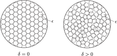
Figure 4: Illustration of the $(\epsilon,\delta)$-capacity in terms of packing $\epsilon$-balls with maximum overlap $\delta$.

In the definition of capacity, we have restricted $\delta<m_{\mathscr{Y}}(V_{\epsilon})$ to rule out the case when the decoding error can be at least as large as the error introduced by the channel, and the $(\epsilon,\delta)$-capacity is infinite. Also, note that $m_{\mathscr{Y}}(V_{\epsilon})\leq 1$ since $V_{\epsilon}\subseteq\mathscr{Y}$ and (9) holds.

We now relate our operational definition of capacity to the notion of UVs and mutual information introduced in Section IV. Let $X$ be the UV corresponding to the transmitted codeword. This is a map $X:\mathscr{X}\to\mathcal{X}$ and $\llbracket X\rrbracket=\mathcal{X}\subseteq\mathscr{X}$. Likewise, let $Y$ be the UV corresponding to the received codeword. This is a map $Y:\mathscr{Y}\to\mathcal{Y}$ and $\llbracket Y\rrbracket=\mathcal{Y}\subseteq\mathscr{Y}$. For our $\epsilon$-perturbation channel, these UVs are such that for all $y\in\llbracket Y\rrbracket$ and $x\in\llbracket X\rrbracket$, we have

$$\llbracket Y|x\rrbracket =\{y\in\llbracket Y\rrbracket:\|x-y\|\leq\epsilon\},$$ (57)

$$\llbracket X|y\rrbracket =\{x\in\llbracket{X}\rrbracket:\|x-y\|\leq\epsilon\},$$ (58)

see Figure 5. Clearly, the set in (57) is continuous, while the set in (58) is discrete.

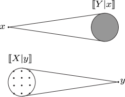
Figure 5: Conditional ranges $\llbracket Y|x\rrbracket$ and $\llbracket X|y\rrbracket$ due to the $\epsilon$-perturbation channel.

To measure the levels of association and disassociation between $X$ and $Y$, we use an uncertainty function $m_{\mathscr{X}}(.)$ defined over $\mathscr{X}$, and $m_{\mathscr{Y}}(.)$ defined over $\mathscr{Y}$. We introduce the feasible set

$$\begin{split}\mathscr{F}_{\delta}&=\{X:\llbracket X\rrbracket\subseteq\mathscr{X},\mbox{ and either }\\ &\qquad(X,Y)\stackrel{{\scriptstyle d}}{{\leftrightarrow}}(0,{{\delta}}/|\llbracket X\rrbracket|)\\ &\qquad\mbox{ or }(X,Y)\stackrel{{\scriptstyle a}}{{\leftrightarrow}}(1,{{\delta}}/|\llbracket X\rrbracket|)\},\end{split}$$ (59)

representing the set of UVs $X$ such that the marginal range $\llbracket X\rrbracket$ is a discrete set representing a codebook, and the UV can either achieve $(0,\delta/|\llbracket X\rrbracket|)$ levels of disassociation or $(1,\delta/|\llbracket X\rrbracket|)$ levels of association with $Y$. In our channel model, this feasible set also depends on the $\epsilon$-perturbation through (57) and (58).

We can now state the non-stochastic channel coding theorem for our $\epsilon$-perturbation channel.

Theorem 4.

For any totally bounded, normed metric space $\mathscr{X}$, $\epsilon$-perturbation channel satisfying (57) and (58), $0<\epsilon\leq 1$ and $0\leq\delta<m_{\mathscr{Y}}(V_{\epsilon})$, we have

$$C_{\epsilon}^{\delta}=\sup_{X\in\mathscr{F}_{\tilde{\delta}},\tilde{\delta}\leq\delta/m_{\mathscr{Y}}(\llbracket Y\rrbracket)}I_{\tilde{\delta}/|\llbracket X\rrbracket|}(Y;X)\mbox{ bits}.$$ (60)

Proof.

First, we show that there exists a UV $X$ and $\tilde{\delta}\leq\delta/m_{\mathscr{Y}}(\llbracket Y\rrbracket)$ such that ${X}\in\mathscr{F}_{\tilde{\delta}}$, which implies that the supremum is well defined. Second, for all $X$ and $\tilde{\delta}$ such that

$$X\in\mathscr{F}_{\tilde{\delta}},$$ (61)

and

$$\tilde{\delta}\leq\delta/m_{\mathscr{Y}}(\llbracket Y\rrbracket),$$ (62)

we show that

$$I_{\tilde{\delta}/|\llbracket X\rrbracket|}(Y;X)\leq C_{\epsilon}^{\delta}.$$ (63)

Finally, we show the existence of $X\in\mathscr{F}_{\tilde{\delta}}$ and $\tilde{\delta}\leq\delta/m_{\mathscr{Y}}(\llbracket Y\rrbracket)$ such that $I_{\tilde{\delta}/|\llbracket X\rrbracket|}(Y;X)=C_{\epsilon}^{\delta}$.

Let us begin with the first step. Consider a point $x\in\mathscr{X}$. Let $X$ be a UV such that

$$\llbracket X\rrbracket=\{x\}.$$ (64)

Then, we have that the marginal range of the UV $Y$ corresponding to the received variable is

$$\llbracket Y\rrbracket=\llbracket Y|x\rrbracket,$$ (65)

and therefore for all $y\in\llbracket Y\rrbracket$, we have

$$\llbracket X|y\rrbracket=\{x\}.$$ (66)

Using Definition 2 and (64), we have that

$$\mathscr{A}(Y;X)=\emptyset,$$ (67)

because $\llbracket X\rrbracket$ consists of a single point, and therefore the set in (11) is empty.

On the other hand, using Definition 2 and (66), we have

$$\mathscr{A}(X;Y)=\begin{cases}\{1\}\mbox{ if $\exists y_{1},y_{2}\in\llbracket Y\rrbracket$,}\\ \emptyset\quad\mbox{ otherwise}.\end{cases}$$ (68)

Using (67) and since $\mathscr{A}\preceq\delta$ holds for $\mathscr{A}=\emptyset$, we have

$$\mathscr{A}(Y;X)\preceq\delta/(|\llbracket X\rrbracket|m_{\mathscr{Y}}(\llbracket Y\rrbracket)).$$ (69)

Similarly, using (68), we have

$$\mathscr{A}(X;Y)\preceq 1.$$ (70)

Now, combining (69) and (70), we have

$$(X,Y)\stackrel{{\scriptstyle a}}{{\leftrightarrow}}(1,\delta/(|\llbracket X\rrbracket|m_{\mathscr{Y}}(\llbracket Y\rrbracket))).$$ (71)

Letting $\tilde{\delta}=\delta/m_{\mathscr{Y}}(\llbracket Y\rrbracket)$, this implies that $X\in\mathscr{F}_{\tilde{\delta}}$ and the first step of the proof is complete.

To prove the second step, we define the set of discrete UVs

$$\begin{split}\mathscr{G}&=\{X:\llbracket X\rrbracket\subseteq\mathscr{X},\exists\tilde{\delta}\leq\delta/m_{\mathscr{Y}}(\llbracket Y\rrbracket)\\ &\qquad\qquad\mbox{ such that }\forall\mathscr{S}_{1},\mathscr{S}_{2}\in\llbracket Y|X\rrbracket,\\ &\qquad\qquad m_{\mathscr{Y}}(\mathscr{S}_{1}\cap\mathscr{S}_{2})/m_{\mathscr{Y}}(\llbracket Y\rrbracket)\leq\tilde{\delta}/|\llbracket X\rrbracket|\},\end{split}$$ (72)

which is a larger set than the one containing all UVs $X$ that are $(1,\tilde{\delta}/|\llbracket X\rrbracket|)$ associated to $Y$. Now, we will show that if an UV $X\in\mathscr{G}$, then the corresponding codebook $\mathcal{X}\in\mathscr{X}_{\epsilon}^{\delta}$. If $X\in\mathscr{G}$, then there exists a $\tilde{\delta}\leq\delta/m_{\mathscr{Y}}(\llbracket Y\rrbracket)$ such that for all $\mathscr{S}_{1},\mathscr{S}_{2}\in\llbracket Y|X\rrbracket$ we have

$$\frac{m_{\mathscr{Y}}(\mathscr{S}_{1}\cap\mathscr{S}_{2})}{m_{\mathscr{Y}}(\llbracket Y\rrbracket)}\leq\frac{\tilde{\delta}}{|\llbracket X\rrbracket|}.$$ (73)

It follows that for all $x_{1},x_{2}\in\llbracket X\rrbracket$, we have

$$\frac{m_{\mathscr{Y}}(\llbracket Y|x_{1}\rrbracket\cap\llbracket Y|x_{2}\rrbracket)}{m_{\mathscr{Y}}(\llbracket Y\rrbracket)}\leq\frac{\tilde{\delta}}{|\llbracket{X}\rrbracket|}.$$ (74)

Using $\mathcal{X}=\llbracket X\rrbracket$, (57), $\llbracket Y\rrbracket=\mathcal{Y}=\bigcup_{x\in\mathcal{X}}S_{\epsilon}(x)$ and $m_{\mathscr{Y}}(\mathscr{Y})=1$, for all $x_{1},x_{2}\in\mathcal{X}$ we have

$$\begin{split}\frac{m_{\mathscr{Y}}(S_{\epsilon}(x_{1})\cap S_{\epsilon}(x_{2}))}{m_{\mathscr{Y}}(\mathscr{Y})}&\leq\frac{\tilde{\delta}m_{\mathscr{Y}}(\llbracket Y\rrbracket)}{|\mathcal{X}|},\\ &\stackrel{{\scriptstyle(a)}}{{\leq}}\frac{\delta}{|\mathcal{X}|},\end{split}$$ (75)

where $(a)$ follows from $\tilde{\delta}\leq\delta/m_{\mathscr{Y}}(\llbracket Y\rrbracket)$. Putting things together, it follows that

$$X\in\mathscr{G}\implies\mathcal{X}\in\mathscr{X}_{\epsilon}^{\delta}$$ (76)

Consider now a pair $X$ and $\tilde{\delta}$ such that $\tilde{\delta}\leq\delta/m_{\mathscr{Y}}(\llbracket Y\rrbracket)$ and

$$X\in\mathscr{F}_{\tilde{\delta}}.$$ (77)

If $(X,Y)\stackrel{{\scriptstyle d}}{{\leftrightarrow}}(0,\tilde{\delta}/|\llbracket X\rrbracket|)$, then using Lemma 3 in Appendix -D there exist two UVs $\bar{X}$ and $\bar{Y}$, and $\bar{\delta}\leq\delta/m_{\mathscr{Y}}(\llbracket\bar{Y}\rrbracket)$ such that

$$(\bar{X},\bar{Y})\stackrel{{\scriptstyle a}}{{\leftrightarrow}}(1,\bar{\delta}/|\llbracket\bar{X}\rrbracket|),$$ (78)

and

$$|\llbracket Y|X\rrbracket^{*}_{\tilde{\delta}/|\llbracket X\rrbracket|}|=|\llbracket\bar{Y}|\bar{X}\rrbracket_{\bar{\delta}/|\llbracket\bar{X}\rrbracket|}^{*}|.$$ (79)

On the other hand, if $(X,{Y})\stackrel{{\scriptstyle a}}{{\leftrightarrow}}(1,\tilde{\delta}/|\llbracket{X}\rrbracket|)$, then (78) and (79) also trivially hold. It then follows that (78) and (79) hold for all $X\in\mathscr{F}_{\tilde{\delta}}$. We now have

$$\begin{split}I_{\tilde{\delta}/|\llbracket X\rrbracket|}(Y;X)&=\log(|\llbracket Y|X\rrbracket_{\tilde{\delta}/|\llbracket X\rrbracket|}^{*}|)\\ &\stackrel{{\scriptstyle(a)}}{{=}}\log(|\llbracket\bar{Y}|\bar{X}\rrbracket_{\bar{\delta}/|\llbracket\bar{X}\rrbracket|}^{*}|)\\ &\stackrel{{\scriptstyle(b)}}{{\leq}}\log(|\llbracket\bar{X}\rrbracket|),\\ &\stackrel{{\scriptstyle(c)}}{{=}}\log(|\bar{\mathcal{X}}|),\\ &\stackrel{{\scriptstyle(d)}}{{\leq}}C^{\delta}_{\epsilon},\end{split}$$ (80)

where $(a)$ follows from (78) and (79), $(b)$ follows from Lemma 5 in Appendix -D since $\bar{\delta}\leq\delta/m_{\mathscr{Y}}(\llbracket\bar{Y}\rrbracket)<m_{\mathscr{Y}}(V_{\epsilon})/m_{\mathscr{Y}}(\llbracket\bar{Y}\rrbracket)$, $(c)$ follows by defining the codebook $\bar{\mathcal{X}}$ corresponding to the UV $\bar{X}$, and $(d)$ follows from the fact that using (78) and Lemma 1, we have $\bar{X}\in\mathcal{G}$, which implies by (76) that $\bar{\mathcal{X}}\in\mathscr{X}_{\epsilon}^{\delta}$.

Finally, let

$$\mathcal{{X}}^{*}=\mbox{argsup}_{\mathcal{X}\in\mathscr{X}_{\epsilon}^{\delta}}\log(|\mathcal{X}|),$$ (81)

which achieves the capacity $C_{\epsilon}^{\delta}$. Let ${{X}}^{*}$ be the UV whose marginal range corresponds to the codebook $\mathcal{{X}}^{*}$. It follows that for all $\mathscr{S}_{1},\mathscr{S}_{1}\in\llbracket Y^{*}|{X}^{*}\rrbracket$, we have

$$\frac{m_{\mathscr{Y}}(\mathscr{S}_{1}\cap\mathscr{S}_{1})}{m_{\mathscr{Y}}(\mathscr{Y})}\leq\frac{\delta}{|\llbracket X^{*}\rrbracket|},$$ (82)

which implies using the fact that $m_{\mathscr{Y}}(\mathscr{Y})=1$,

$$\frac{m_{\mathscr{Y}}(\mathscr{S}_{1}\cap\mathscr{S}_{1})}{m_{\mathscr{Y}}(\llbracket Y^{*}\rrbracket)}\leq\frac{\delta}{|\llbracket X^{*}\rrbracket|m_{\mathscr{Y}}(\llbracket Y^{*}\rrbracket)}.$$ (83)

Letting $\delta^{*}=\delta/m_{\mathscr{Y}}(\llbracket Y^{*}\rrbracket)$, and using Lemma 1, we have that $(X^{*},{Y}^{*})\stackrel{{\scriptstyle a}}{{\leftrightarrow}}(1,\delta^{*}/|\llbracket X^{*}\rrbracket|)$, which implies ${{X}^{*}}\in\cup_{\tilde{\delta}\leq\delta/m_{\mathscr{Y}}(\llbracket Y^{*}\rrbracket}\mathscr{F}_{\tilde{\delta}}$ and the proof is complete.

∎

Theorem 4 characterizes the capacity as the supremum of the mutual information over all UVs in the feasible set. The following theorem shows that the same characterization is obtained if we optimize the right hand side in (60) over all UVs in the space. It follows that by Theorem 4, rather than optimizing over all UVs representing all the codebooks in the space, a capacity achieving codebook can be found within the smaller class $\cup_{\tilde{\delta}\leq\delta/m_{\mathscr{Y}}(V_{\epsilon})}\mathscr{F}_{\tilde{\delta}}$ of feasible sets with error at most $\delta/m_{\mathscr{Y}}(V_{\epsilon})$, since for all $\llbracket Y\rrbracket\subseteq\mathscr{Y}$, $m_{\mathscr{Y}}(V_{\epsilon})\leq m_{\mathscr{Y}}(\llbracket Y\rrbracket)$.

Theorem 5.

The $(\epsilon,\delta)$-capacity in (60) can also be written as

$$C_{\epsilon}^{\delta}=\sup_{\begin{subarray}{c}X:\llbracket X\rrbracket\subseteq\mathscr{X},\\ \tilde{\delta}\leq\delta/m_{\mathscr{Y}}(\llbracket Y\rrbracket)\end{subarray}}I_{\tilde{\delta}/|\llbracket X\rrbracket|}(Y;X)\mbox{ bits}.$$ (84)

Proof.

Consider an UV $X\not\in\cup_{\tilde{\delta}\leq\delta/m_{\mathscr{Y}}(\llbracket Y\rrbracket)}\mathscr{F}_{\tilde{\delta}}$, where $Y$ is the corresponding UV at the receiver. The idea of the proof is to show the existence of an UV $\bar{X}\in\cup_{\tilde{\delta}\leq\delta/m_{\mathscr{Y}}(\llbracket\bar{Y}\rrbracket)}\mathscr{F}_{\tilde{\delta}}$ and the corresponding UV $\bar{Y}$ at the receiver, and

$$\bar{\delta}=\tilde{\delta}m_{\mathscr{Y}}(\llbracket{Y}\rrbracket)/m_{\mathscr{Y}}(\llbracket\bar{Y}\rrbracket)\leq\delta/m(\llbracket\bar{Y}\rrbracket),$$ (85)

such that the cardinality of the overlap partitions

$$|\llbracket\bar{Y}|\bar{X}\rrbracket^{*}_{\bar{\delta}/|\llbracket\bar{X}\rrbracket|}|=|\llbracket Y|{X}\rrbracket^{*}_{\tilde{\delta}/|\llbracket X\rrbracket|}|.$$ (86)

Let the cardinality

$$|\llbracket Y|X\rrbracket_{{\tilde{\delta}}/|\llbracket X\rrbracket|}^{*}|=K.$$ (87)

By Property 1 of Definition 6, we have that for all $\mathscr{S}_{i}\in\llbracket Y|X\rrbracket_{\tilde{\delta}/|\llbracket X\rrbracket|}^{*}$, there exists an $x_{i}\in\llbracket X\rrbracket$ such that $\llbracket Y|x_{i}\rrbracket\subseteq\mathscr{S}_{i}$. Now, consider another UV $\bar{X}$ whose marginal range is composed of $K$ elements of $\llbracket{X}\rrbracket$, namely

$$\llbracket\bar{X}\rrbracket=\{x_{1},\ldots x_{K}\}.$$ (88)

Let $\bar{Y}$ be the UV corresponding to the received variable. Using the fact that for all $x\in\mathscr{X}$, we have $\llbracket\bar{Y}|x\rrbracket=\llbracket{Y}|x\rrbracket$ since (57) holds, and using Property 2 of Definition 6, for all $x,x^{\prime}\in\llbracket\bar{X}\rrbracket$, we have that

$$\begin{split}\frac{m_{\mathscr{Y}}(\llbracket\bar{Y}|x\rrbracket\cap\llbracket\bar{Y}|x^{\prime}\rrbracket)}{m_{\mathscr{Y}}(\llbracket{Y}\rrbracket)}&\leq\frac{\tilde{\delta}}{|\llbracket X\rrbracket|},\\ &\stackrel{{\scriptstyle(a)}}{{\leq}}\frac{\tilde{\delta}}{|\llbracket\bar{X}\rrbracket|},\end{split}$$ (89)

where $(a)$ follows from the fact that $\llbracket\bar{X}\rrbracket\subseteq\llbracket X\rrbracket$ using (88). Then, for all $x,x^{\prime}\in\llbracket\bar{X}\rrbracket$, we have that

$$\begin{split}\frac{m_{\mathscr{Y}}(\llbracket\bar{Y}|x\rrbracket\cap\llbracket\bar{Y}|x^{\prime}\rrbracket)}{m_{\mathscr{Y}}(\llbracket\bar{Y}\rrbracket)}&\leq\frac{\tilde{\delta}m_{\mathscr{Y}}(\llbracket{Y}\rrbracket)}{|\llbracket\bar{X}\rrbracket|m_{\mathscr{Y}}(\llbracket\bar{Y}\rrbracket)}\\ &=\frac{\bar{\delta}}{|\llbracket\bar{X}\rrbracket|},\end{split}$$ (90)

since $\bar{\delta}=\tilde{\delta}m_{\mathscr{Y}}(\llbracket{Y}\rrbracket)/m_{\mathscr{Y}}(\llbracket\bar{Y}\rrbracket)$. Then, by Lemma 1 it follows that

$$(\bar{X},\bar{Y})\stackrel{{\scriptstyle a}}{{\leftrightarrow}}(1,\bar{\delta}/|\llbracket\bar{X}\rrbracket|).$$ (91)

Since $\tilde{\delta}\leq\delta/m_{\mathscr{Y}}(\llbracket{Y}\rrbracket)$, we have

$$\bar{\delta}\leq\delta/m_{\mathscr{Y}}(\llbracket\bar{Y}\rrbracket)<m_{\mathscr{Y}}(V_{\epsilon})/m_{\mathscr{Y}}(\llbracket\bar{Y}\rrbracket).$$ (92)

Therefore, $\bar{X}\in\mathscr{F}_{\bar{\delta}}$ and $\bar{\delta}\leq\delta/m_{\mathscr{Y}}(\llbracket\bar{Y}\rrbracket)$. We now have that

$$\begin{split}|\llbracket\bar{Y}|\bar{X}\rrbracket^{*}_{\bar{\delta}/|\llbracket\bar{X}\rrbracket|}|&\stackrel{{\scriptstyle(a)}}{{=}}|\llbracket\bar{X}\rrbracket|\\ &\stackrel{{\scriptstyle(b)}}{{=}}|\llbracket Y|X\rrbracket_{{\tilde{\delta}}/|\llbracket X\rrbracket|}^{*}|,\end{split}$$ (93)

where $(a)$ follows by applying Lemma 6 in Appendix -D using (91) and (92), and $(b)$ follows from (87) and (88). Combining (93) with Theorem 4, the proof is complete. ∎

Finally, we make some considerations with respect to previous results in the literature. First, we note that for $\delta=0$, all of our definitions reduce to Nair’s ones and Theorem 4 recovers Nair’s coding theorem [3, Theorem 4.1] for the zero-error capacity of an additive $\epsilon$-perturbation channel.

Second, we point out that the $(\epsilon,\delta)$-capacity considered in [11] defines the set of $(\epsilon,\delta)$-distinguishable codewords such that the average overlap among all codewords is at most $\delta$. In contrast, our definition requires the overlap for each pair of codewords to be at most $\delta/|\mathcal{X}|$. The following theorem provides the relationship between our $C_{\epsilon}^{\delta}$ and the capacity $\tilde{C}_{\epsilon}^{\delta}$ considered in [11], which is defined using the Euclidean norm.

Theorem 6.

Let $\tilde{C}_{\epsilon}^{\delta}$ be the $(\epsilon,\delta)$-capacity defined in [11]. We have

$$C_{\epsilon}^{\delta}\leq\tilde{C}_{\epsilon}^{\delta/(2m_{\mathscr{Y}}(V_{\epsilon}))},$$ (94)

and

$$\tilde{C}^{\delta}_{\epsilon}\leq{C}^{\delta m_{\mathscr{Y}}(V_{\epsilon})2^{2\tilde{C}^{\delta}_{\epsilon}+1}}_{\epsilon}.$$ (95)

Proof.

For every codebook $\mathcal{X}\in\mathscr{X}^{\delta}_{\epsilon}$ and $x_{1},x_{2}\in\mathcal{X}$, we have

$$e_{\epsilon}(x_{1},x_{2})\leq\delta/|\mathcal{X}|.$$ (96)

Since $m_{\mathscr{Y}}(\mathscr{Y})=1$, this implies that for all $x_{1},x_{2}\in\mathcal{X}$, we have

$$\begin{split}m_{\mathscr{Y}}(S_{\epsilon}(x_{1})\cap S_{\epsilon}(x_{2}))&\leq\delta/|\mathcal{X}|.\end{split}$$ (97)

For all $\mathcal{X}\in\mathscr{X}$, the average overlap defined in [11, (53)] is

$$\Delta=\frac{1}{|\mathcal{X}|}\sum_{x\in\mathcal{X}}\frac{e_{\epsilon}(x)}{2m_{\mathscr{Y}}(V_{\epsilon})}.$$ (98)

Then, we have

$$\begin{split}\Delta&=\frac{1}{2|\mathcal{X}|m_{\mathscr{Y}}(V_{\epsilon})}\sum_{x_{1},x_{2}\in\mathcal{X}}m_{\mathscr{Y}}(S_{\epsilon}(x_{1})\cap S_{\epsilon}(x_{2})),\\ &\stackrel{{\scriptstyle(a)}}{{\leq}}\frac{\delta|\mathcal{X}|^{2}}{2|\mathcal{X}|^{2}m_{\mathscr{Y}}(V_{\epsilon})},\\ &\leq\frac{\delta}{2m_{\mathscr{Y}}(V_{\epsilon})},\end{split}$$ (99)

where $(a)$ follows from (97). Thus, we have

$$C_{\epsilon}^{\delta}\leq\tilde{C}_{\epsilon}^{\delta/(2m_{\mathscr{Y}}(V_{\epsilon}))},$$ (100)

and (94) follows.

Now, let $\mathcal{X}$ be a codebook with average overlap at most $\delta$, namely

$$\frac{1}{2|\mathcal{X}|m_{\mathscr{Y}}(V_{\epsilon})}\sum_{x_{1},x_{2}\in\mathcal{X}}m_{\mathscr{Y}}(S_{\epsilon}(x_{1})\cap S_{\epsilon}(x_{2}))\leq\delta.$$ (101)

This implies that for all $x_{1},x_{2}\in\mathcal{X}$, we have

$$\begin{split}\frac{|\mathcal{X}|m_{\mathscr{Y}}(S_{\epsilon}(x_{1})\cap S_{\epsilon}(x_{2}))}{m_{\mathscr{Y}}(\mathscr{Y})}&\leq\frac{2\delta|\mathcal{X}|^{2}m_{\mathscr{Y}}(V_{\epsilon})}{m_{\mathscr{Y}}(\mathscr{Y})},\\ &\stackrel{{\scriptstyle(a)}}{{=}}{2\delta|\mathcal{X}|^{2}m_{\mathscr{Y}}(V_{\epsilon})},\\ &\leq{\delta 2^{2\tilde{C}^{\delta}_{\epsilon}+1}}m_{\mathscr{Y}}(V_{\epsilon}),\end{split}$$ (102)

where $(a)$ follows from the fact that $m_{\mathscr{Y}}(\mathscr{Y})=1$. Thus, we have

$$\tilde{C}^{\delta}_{\epsilon}\leq{C}^{\delta 2^{2\tilde{C}^{\delta}_{\epsilon}+1}m_{\mathscr{Y}}(V_{\epsilon})}_{\epsilon},$$ (103)

and (95) follows. ∎

VI $(N,\delta)$-Capacity of General Channels

We now extend our results to more general channels where the noise can be different across codewords, and not necessarily contained within a ball of radius $\epsilon$.

Let $\mathcal{X}\subseteq\mathscr{X}$ be a discrete set of points in the space, which represents a codebook. Any point $x\in\mathcal{X}$ represents a codeword that can be selected at the transmitter, sent over the channel, and received with perturbation. A channel with transition mapping $N:\mathscr{X}\to\mathscr{Y}$ associates to any point in $\mathscr{X}$ a set in $\mathscr{Y}$, such that the received codeword lies in the set

$$S_{N}(x)=\{y\in\mathscr{Y}:y\in N(x)\}.$$ (104)

Figure 6 illustrates possible uncertainty sets associated to three different codewords.

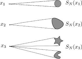
Figure 6: Uncertainty sets associated to three different codewords. Sets are not necessarily balls, they can be different across codewords, and also be composed of disconnected subsets.

All received codewords lie in the set $\mathcal{Y}=\bigcup_{x\in\mathcal{X}}S_{N}(x)$, where $\mathcal{Y}\subseteq\mathscr{Y}$. For any $x_{1},x_{2}$ $\in$ $\mathcal{X}$, we now let

$$e_{N}(x_{1},x_{2})=\frac{m_{\mathscr{Y}}(S_{N}(x_{1})\cap S_{N}(x_{2}))}{m_{\mathscr{Y}}(\mathscr{Y})},$$ (105)

where $m_{\mathscr{Y}}(.)$ is an uncertainty function defined over $\mathscr{Y}$. We also assume without loss of generality that the uncertainty associated with the space $\mathscr{Y}$ of received codewords is $m_{\mathscr{Y}}(\mathscr{Y})=1$. We also let $V_{N}=N(x^{*})$, where $x^{*}=\mbox{argmin}_{x\in\mathscr{X}}m_{\mathscr{Y}}(N(x))$. Thus, $V_{N}$ is the set corresponding to the minimum uncertainty introduced by the noise mapping $N$.

Definition 11.

$(N,\delta)$-distinguishable codebook.
For any $0\leq\delta<m_{\mathscr{Y}}(V_{N})$, a codebook $\mathcal{X}\subseteq\mathscr{X}$ is $(N,\delta)$-distinguishable if for all $x_{1},x_{2}\in\mathcal{X}$, we have $e_{N}(x_{1},x_{2})\leq\delta/|\mathcal{X}|$.

Definition 12.

$(N,\delta)$-capacity.
For any totally bounded, normed metric space $\mathscr{X}$, channel with transition mapping $N$, and $0\leq\delta<m_{\mathscr{Y}}(V_{N})$, the $(N,\delta)$-capacity of $\mathscr{X}$ is

$$C_{N}^{\delta}=\sup_{\mathcal{X}\in\mathscr{X}_{N}^{\delta}}\log_{2}|\mathcal{X}|\mbox{ bits},$$ (106)

where $\mathscr{X}_{N}^{\delta}=\{\mathcal{X}:\mathcal{X}\mbox{ is }(N,\delta)\mbox{-distinguishable}\}$.

We now relate our operational definition of capacity to the notion of UVs and mutual information introduced in Section IV. As usual, let $X$ be the UV corresponding to the transmitted codeword and $Y$ be the UV corresponding to the received codeword. For a channel with transition mapping $N$, these UVs are such that for all $y\in\llbracket Y\rrbracket$ and $x\in\llbracket X\rrbracket$, we have

$$\llbracket Y|x\rrbracket =\{y\in\llbracket Y\rrbracket:y\in N(x)\},$$ (107)

$$\llbracket X|y\rrbracket =\{x\in\llbracket{X}\rrbracket:y\in N(x)\}.$$ (108)

To measure the levels of association and disassociation between UVs $X$ and $Y$, we use an uncertainty function $m_{\mathscr{X}}(.)$ defined over $\mathscr{X}$, and $m_{\mathscr{Y}}(.)$ is defined over $\mathscr{Y}$. The definition of feasible set is the same as the one given in (59). In our channel model, this feasible set depends on the transition mapping $N$ through (107) and (108).

We can now state the non-stochastic channel coding theorem for channels with transition mapping $N$.

Theorem 7.

For any totally bounded, normed metric space $\mathscr{X}$, channel with transition mapping $N$ satisfying (107) and (108), and $0\leq\delta<m_{\mathscr{Y}}(V_{N})$, we have

$$C_{N}^{\delta}=\sup_{X\in\mathscr{F}_{\tilde{\delta}},\tilde{\delta}\leq\delta/m_{\mathscr{Y}}(\llbracket Y\rrbracket)}I_{\tilde{\delta}/|\llbracket X\rrbracket|}(Y;X)\;\mbox{ bits}.$$ (109)

The proof is along the same lines as the one of Theorem 4 and is omitted.

Theorem 7 characterizes the capacity as the supremum of the mutual information over all codebooks in the feasible set. The following theorem shows that the same characterization is obtained if we optimize the right hand side in (109) over all codebooks in the space. It follows that by Theorem 7, rather than optimizing over all codebooks, a capacity achieving codebook can be found within the smaller class $\cup_{\tilde{\delta}\leq\delta/m_{\mathscr{Y}}(V_{N})}\mathscr{F}_{\tilde{\delta}}$ of feasible sets with error at most $\delta/m_{\mathscr{Y}}(V_{N})$.

Theorem 8.

The $(N,\delta)$-capacity in (109) can also be written as

$$C_{N}^{\delta}=\sup_{\begin{subarray}{c}X:\llbracket X\rrbracket\subseteq\mathscr{X},\\ \tilde{\delta}\leq\delta/m_{\mathscr{Y}}(\llbracket Y\rrbracket)\end{subarray}}I_{\tilde{\delta}/|\llbracket X\rrbracket|}(Y;X)\mbox{ bits}.$$ (110)

The proof is along the same lines as the one of Theorem 5 and is omitted.

VII Capacity of Stationary Memoryless Uncertain Channels

We now consider the special case of stationary, memoryless, uncertain channels.

Let $\mathscr{X}^{\infty}$ be the space of $\mathscr{X}$-valued discrete-time functions $x:\mathbb{Z}_{>0}\to\mathscr{X}$, where $\mathbb{Z}_{>0}$ is the set of positive integers denoting the time step. Let $x(a:b)$ denote the function $x\in\mathscr{X}^{\infty}$ restricted over the time interval $[a,b]$. Let $\mathcal{X}\subseteq\mathscr{X}^{\infty}$ be a discrete set which represents a codebook. Also, let $\mathcal{X}(1:n)=\cup_{x\in\mathcal{X}}x(1:n)$ denote the set of all codewords up to time $n$, and $\mathcal{X}(n)=\cup_{x\in\mathcal{X}}x(n)$ the set of all codeword symbols in the codebook at time $n$. The codeword symbols can be viewed as the coefficients representing a continuous signal in an infinite-dimensional space. For example, transmitting one symbol per time step can be viewed as transmitting a signal of unit spectral support over time. The perturbation of the signal at the receiver due to the noise can be described as a displacement experienced by the corresponding codeword symbols $x(1),x(2),\ldots$. To describe this perturbation we consider the set-valued map $N^{\infty}:\mathscr{X}^{\infty}\to\mathscr{Y}^{\infty}$, associating any point in $\mathscr{X}^{\infty}$ to a set in $\mathscr{Y}^{\infty}$. For any transmitted codeword $x\in\mathcal{X}\subseteq\mathscr{X}^{\infty}$, the corresponding received codeword lies in the set

$$S_{N^{\infty}}(x)=\{y\in\mathscr{Y}^{\infty}:y\in N^{\infty}(x)\}.$$ (111)

Additionally, the noise set associated to $x(1:n)\in\mathcal{X}(1:n)$ is

$$S_{N^{\infty}}(x(1:n))=\{y(1:n)\in\mathscr{Y}^{n}:y\in N^{\infty}(x)\},$$ (112)

where

$$\mathscr{Y}^{n}=\underbrace{\mathscr{Y}\times\mathscr{Y}\times\cdots\times\mathscr{Y}}_{n}.$$ (113)

We are now ready to define stationary, memoryless, uncertain channels.

Definition 13.

A stationary memoryless uncertain channel is a transition mapping $N^{\infty}:\mathscr{X}^{\infty}\to\mathscr{Y}^{\infty}$ that can be factorized into identical terms describing the noise experienced by the codeword symbols. Namely, there exists a set-valued map $N:\mathscr{X}\to\mathscr{Y}$ such that for all $n\in\mathbb{Z}_{>0}$ and $x(1:n)\in\mathscr{X}^{\infty}$, we have

$$S_{N^{\infty}}(x(1:n))=N(x(1))\times\ldots\times N(x(n)).$$ (114)

According to the definition, a stationary memoryless uncertain channel maps the $n$th input symbol into the $n$th output symbol in a way that does not depend on the symbols at other time steps, and the mapping is the same at all time steps. Since the channel can be characterized by the mapping $N$ instead of $N^{\infty}$, to simplify the notation in the following we use $S_{N}(.)$ instead of $S_{N^{\infty}}(.)$.

Another important observation is that the $\epsilon$-noise channel that we considered in Section V may not admit a factorization like the one in (114). For example, consider the space to be equipped with the $L^{2}$ norm, the codeword symbols to represent the coefficients of an orthogonal representation of a transmitted signal, and the noise experienced by any codeword to be within a ball of radius $\epsilon$. In this case, if a codeword symbol is perturbed by a value close to $\epsilon$ the perturbation of all other symbols must be close to zero. On the other hand, the general channels considered in Section VI can be stationary and memoryless, if the noise acts on the coefficients in a way that satisfies (114).

For stationary memoryless uncertain channels, all received codewords lie in the set $\mathcal{Y}=\cup_{x\in\mathcal{X}}S_{N}(x)$, and the received codewords up to time $n$ lie in the set $\mathcal{Y}(1:n)=\cup_{x\in\mathcal{X}}S_{N}(x(1:n))$. Then, for any $x_{1}(1:n),x_{2}(1:n)\in\mathcal{X}(1:n)$, we let

$$\begin{split}&e_{N}(x_{1}(1:n),x_{2}(1:n))\\ &=\frac{m_{\mathscr{Y}}(S_{N}(x_{1}(1:n))\cap S_{N}(x_{2}(1:n)))}{m_{\mathscr{Y}}(\mathscr{Y}^{n})}.\end{split}$$ (115)

We also assume without loss of generality that at any time step $n$, the uncertainty associated to the space $\mathscr{Y}^{n}$ of received codewords is $m_{\mathscr{Y}}(\mathscr{Y}^{n})=1$. We also let $V_{N}=N(x^{*})$, where $x^{*}=\mbox{argmin}_{x\in\mathscr{X}}m_{\mathscr{Y}}(N(x))$. Thus, $V_{N}$ is the set corresponding to the minimum uncertainty introduced by the noise mapping at a single time step. Finally, we let

$$V_{N}^{n} =\underbrace{V_{N}\times V_{N}\times\cdots\times V_{N}}_{n}.$$ (116)

Definition 14.

$(N,\delta_{n})$-distinguishable codebook.
For all $n\in\mathbb{Z}_{>0}$ and $0\leq\delta_{n}<m_{\mathscr{Y}}(V_{N}^{n})$, a codebook $\mathcal{X}_{n}=\mathcal{X}(1:n)$ is $(N,\delta_{n})$-distinguishable if for all $x_{1}(1:n),x_{2}(1:n)\in\mathcal{X}_{n}$, we have

$$e_{N}(x_{1}(1:n),x_{2}(1:n))\leq\delta_{n}/|\mathcal{X}_{n}|.$$ (117)

It immediately follows that for any $(N,\delta_{n})$-distinguishable codebook $\mathcal{X}_{n}$, we have

$$e_{N}(x(1:n))=\sum_{\begin{subarray}{c}x^{\prime}(1:n)\in\mathcal{X}_{n}:\\ x^{\prime}(1:n)\neq x(1:n)\end{subarray}}e_{N}(x(1:n),x^{\prime}(1:n))\leq\delta_{n},$$ (118)

so that each codeword in $\mathcal{X}_{n}$ can be decoded correctly with confidence at least $1-\delta_{n}$. Definion 14 guarantees even more namely, that the confidence of not confusing any pair of codewords is at least $1-\delta_{n}/|\mathcal{X}_{n}|$.

We now associate to any sequence $\{\delta_{n}\}$ the largest distinguishable rate sequence $\{R_{\delta_{n}}\}$, whose elements represent the largest rates that satisfy that confidence sequence.

Definition 15.

Largest $\{\delta_{n}\}$-distinguishable rate sequence.
For any sequence $\{\delta_{n}\}$, the largest $\{\delta_{n}\}$-distinguishable rate sequence $\{R_{\delta_{n}}\}$ is such that for all $n\in\mathbb{Z}_{>0}$ we have

$$R_{\delta_{n}}=\sup_{\mathcal{X}_{n}\in\mathscr{X}^{\delta_{n}}_{N}(n)}\frac{\log|\mathcal{X}_{n}|}{n}\mbox{ bits per symbol},$$ (119)

where

$$\mathscr{X}_{N}^{\delta_{n}}(n)=\{\mathcal{X}_{n}:\mathcal{X}_{n}\mbox{ is }(N,\delta_{n})\mbox{-distinguishable}\}.$$ (120)

We say that any constant rate $R$ that lays below the largest $\{\delta_{n}\}$-distinguishable rate sequence is $\{\delta_{n}\}$-distinguishable. Such a $\{\delta_{n}\}$-distinguishable rate ensures the existence of a sequence of distinguishable codes that, for all $n\in\mathbb{Z}_{>0}$, have rate at least $R$ and confidence at least $1-\delta_{n}$.

Definition 16.

$\{\delta_{n}\}$-distinguishable rate.
For any sequence $\{\delta_{n}\}$, a constant rate $R$ is said to be $\{\delta_{n}\}$-distinguishable if for all $n\in\mathbb{Z}_{>0}$, we have

$$R\leq R_{\delta_{n}}.$$ (121)

We call any $\{\delta_{n}\}$-distinguishable rate $R$ achievable, if $\delta_{n}\rightarrow 0$ as $n\rightarrow\infty$. An achievable rate $R$ ensures the existence of a sequence of distinguishable codes of rate at least $R$ whose confidence tends to one as $n\rightarrow\infty$. It follows that in this case we can achieve communication at rate $R$ with arbitrarily high confidence by choosing a sufficiently large codebook.

Definition 17.

Achievable rate.
A constant rate $R$ is achievable if there exists a sequence $\{\delta_{n}\}$ such that $\delta_{n}\rightarrow 0$ as $n\rightarrow\infty$, and $R$ is $\{\delta_{n}\}$-distinguishable.

We now give a first definition of capacity as the supremum of the $\{\delta_{n}\}$-distinguishable rates. Using this definition, transmitting at constant rate below capacity ensures the existence of a sequence of codes that, for all $n\in\mathbb{Z}_{>0}$, have confidence at least $1-\delta_{n}$.

Definition 18.

$(N,\{\delta_{n}\})_{*}$ capacity.
For any stationary memoryless uncertain channel with transition mapping $N$, and any given sequence $\{\delta_{n}\}$, we let

$$C_{N}(\{\delta_{n}\})_{*} =\sup\{R:R\mbox{ is }\{\delta_{n}\}\mbox{-distinguishable}\}$$ (122)

$$=\inf_{n\in\mathbb{Z}_{>0}}R_{\delta_{n}}\;\;\mbox{ bits per symbol}.$$ (123)

Another definition of capacity arises if rather than the largest lower bound to the sequence of rates one considers the least upper bound for which we can transmit satisfying a given confidence sequence. Using this definition, transmitting at constant rate below capacity ensures the existence of a code that satisfies at least one confidence value along the sequence $\{\delta_{n}\}$.

Definition 19.

$(N,\{\delta_{n}\})^{*}$ capacity.
For any stationary memoryless uncertain channel with transition mapping $N$, and any given sequence $\{\delta_{n}\}$, we define

$$C_{N}(\{\delta_{n}\})^{*} =\sup_{n\in\mathbb{Z}_{>0}}R_{\delta_{n}}\;\;\mbox{ bits per symbol}.$$ (124)

Definitions 18 and 19 lead to non-stochastic analogues of Shannon’s probabilistic and zero-error capacities, respectively.

First, consider Definition 18 and take the supremum of the achievable rates, rather than the supremum of the $\{\delta_{n}\}$-distinguishable rates. This means that we can pick any confidence sequence such that $\delta_{n}$ tends to zero as $n\rightarrow\infty$. In this way, we obtain the non-stochastic analogue of Shannon’s probabilistic capacity, where $\delta_{n}$ plays the role of the probability of error and the capacity is the largest rate that can be achieved by a sequence of codebooks with an arbitrarily high confidence level.

Definition 20.

$(N,\{\downarrow 0\})_{*}$ capacity.
For any stationary memoryless uncertain channel with transition mapping $N$, we define the $(N,\{\downarrow 0\})_{*}$ capacity as

$$C_{N}(\{\downarrow 0\})_{*} =\sup\{R:R\mbox{ is achievable}\}$$ (125)

$$=\sup_{\{\delta_{n}\}:\delta_{n}=o(1)}C_{N}(\{\delta_{n}\})_{*}.$$ (126)

Next, consider Definition 19 in the case $\{\delta_{n}\}$ is a constant sequence, namely for all $n\in\mathbb{Z}_{>0}$ we have $\delta_{n}=\delta\geq 0$. In this case, transmitting below capacity ensures the existence of a finite-length code that has confidence at least $1-\delta$.

Definition 21.

$(N,\delta)^{*}$ capacity.
For any stationary memoryless uncertain channel with transition mapping $N$, and any sequence $\{\delta_{n}\}$ such that for all $n\in\mathbb{Z}_{>0}$ we have $\delta_{n}=\delta\geq 0$, we define

$$C_{N}^{\delta*} =\sup_{n\in\mathbb{Z}_{>0}}R_{\delta_{n}}\;\;\mbox{ bits per symbol}.$$ (127)

Letting $\delta=0$, we obtain the zero-error capacity. In this case, below capacity there exists at a code with which we can transmit with full confidence.

We point out the key difference between Definitions 20 and 21. Transmitting below the $(N,\{\downarrow 0\})_{*}$ capacity, allows to achieve arbitrarily high confidence by increasing the codeword size. In contrast, transmitting below the $(N,\delta)^{*}$ capacity, ensures the existence of a fixed codebook that has confidence at least $1-\delta$.

We now relate our notions of capacity to the mutual information rate between transmitted and received codewords. Let $X$ be the UV corresponding to the transmitted codeword. This is a map $X:\mathscr{X}^{\infty}\to\mathcal{X}$ and $\llbracket X\rrbracket=\mathcal{X}\subseteq\mathscr{X}^{\infty}$. Restricting this map to a finite time $n\in\mathbb{Z}_{>0}$ yields another UV $X(n)$ and $\llbracket X(n)\rrbracket=\mathcal{X}(n)\subseteq\mathscr{X}$. Likewise, a codebook segment is an UV $X(a:b)=\{X(n)\}_{a\leq n\leq b}$, of marginal range

$$\llbracket X(a:b)\rrbracket=\mathcal{X}(a:b)\subseteq\mathscr{X}^{b-a+1}.$$ (128)

Likewise, let $Y$ be the UV corresponding to the received codeword. It is a map $Y:\mathscr{Y}^{\infty}\to\mathcal{Y}$ and $\llbracket Y\rrbracket=\mathcal{Y}\subseteq\mathscr{Y}^{\infty}$. $Y(n)$ and $Y(a:b)$ are UVs, and $\llbracket Y(n)\rrbracket=\mathcal{Y}\subseteq\mathscr{Y}^{\infty}$ and $\llbracket Y(a:b)\rrbracket=\mathcal{Y}(a:b)\subseteq\mathscr{Y}^{b-a+1}$. For a stationary memoryless channel with transition mapping $N$, these UVs are such that for all $n\in\mathbb{Z}_{>0}$, $y(1:n)\in\llbracket Y(1:n)\rrbracket$ and $x(1:n)\in\llbracket X(1:n)\rrbracket$, and we have

$$\begin{split}\llbracket Y(1:n)|x(1:n)\rrbracket=&\{y(1:n)\in\llbracket Y(1:n)\rrbracket:\\ &y(1:n)\in S_{N}(x(1:n))\},\end{split}$$ (129)

$$\begin{split}\llbracket X(1:n)|y(1:n)\rrbracket=&\{x(1:n)\in\llbracket X(1:n)\rrbracket:\\ &y(1:n)\in S_{N}(x(1:n))\}.\end{split}$$ (130)

Now, we define the largest $\delta_{n}$-mutual information rate as the supremum mutual information per unit-symbol transmission that a codeword $X(1:n)$ can provide about $Y(1:n)$ with confidence at least $1-\delta_{n}/|\llbracket X(1:n)\rrbracket|$.

Definition 22.

Largest $\delta_{n}$-information rate.
For all $n\in\mathbb{Z}_{>0}$, the largest $\delta_{n}$-information rate from $X(1:n)$ to $Y(1:n)$ is

$$R^{I}_{\delta_{n}}=\sup_{\begin{subarray}{c}X(1:n):\llbracket X(1:n)\rrbracket\subseteq\mathscr{X}^{n},\\ \tilde{\delta}\leq\delta_{n}/m_{\mathscr{Y}}(\llbracket Y(1:n)\rrbracket)\end{subarray}}\frac{I_{\tilde{\delta}/|\llbracket X(1:n)\rrbracket|}(Y(1:n);X(1:n))}{n}.$$ (131)

We let the feasible set at time $n$ be

$$\begin{split}\mathscr{F}_{\delta}(n)&=\{X(1:n):\llbracket X(1:n)\rrbracket\subseteq\mathscr{X}^{n},\mbox{ and either }\\ &(X(1:n),Y(1:n))\stackrel{{\scriptstyle d}}{{\leftrightarrow}}(0,{{\delta}}/|\llbracket X(1:n)\rrbracket|)\mbox{ or}\\ &(X(1:n),Y(1:n))\stackrel{{\scriptstyle a}}{{\leftrightarrow}}(1,{{\delta}}/|\llbracket X(1:n)\rrbracket|)\}.\end{split}$$ (132)

In the following theorem we establish the relationship between $R_{\delta_{n}}$ and $R^{I}_{\delta_{n}}$.

Theorem 9.

For any totally bounded, normed metric space $\mathscr{X}$, disrete-time space $\mathscr{X}^{\infty}$, stationary memoryless uncertain channel with transition mapping $N$ satisfying (129) and (130), and sequence $\{\delta_{n}\}$ such that for all $n\in\mathbb{Z}_{>0}$ we have $0\leq\delta_{n}<m_{\mathscr{Y}}(V_{N}^{n})$, we have

$$R_{\delta_{n}}=\sup_{\begin{subarray}{c}X(1:n)\in\mathscr{F}_{\tilde{\delta}}(n),\\ \tilde{\delta}\leq\delta_{n}/m_{\mathscr{Y}}(\llbracket Y(1:n)\rrbracket)\end{subarray}}\frac{I_{\tilde{\delta}/|\llbracket X(1:n)\rrbracket|}(Y(1:n);X(1:n))}{n}.$$ (133)

We also have

$$R_{\delta_{n}}=R^{I}_{\delta_{n}}.$$ (134)

Proof.

The proof of the theorem is similar to the one of Theorem 4 and is given in Appendix -B. ∎

The following coding theorem is now an immediate consequence of Theorem 9 and of our capacity definitions.

Theorem 10.

For any totally bounded, normed metric space $\mathscr{X}$, disrete-time space $\mathscr{X}^{\infty}$, stationary memoryless uncertain channel with transition mapping $N$ satisfying (129) and (130), and sequence $\{\delta_{n}\}$ such that for all $n\in\mathbb{Z}_{>0}$, $0\leq\delta_{n}<m_{\mathscr{Y}}(V_{N}^{n})$ and $0\leq\delta<m_{\mathscr{Y}}(V_{N}^{n})$, we have

$$1)\;\;\;\; {C}_{N}(\{\delta_{n}\})_{*}=\inf_{n\in\mathbb{Z}_{>0}}R^{I}_{\delta_{n}},$$ (135)

$$2)\;\;\;\; {C}_{N}(\{\delta_{n}\})^{*}=\sup_{n\in\mathbb{Z}_{>0}}R^{I}_{\delta_{n}},$$ (136)

$$3)\;\;\;\; {C}_{N}(\{\downarrow 0\})_{*}=\sup_{\{\delta_{n}\}:\delta_{n}=o(1)}\inf_{n\in\mathbb{Z}_{>0}}R^{I}_{\delta_{n}},$$ (137)

$$4)\;\;\;\; {C}_{N}^{\delta*}=\sup_{n\in\mathbb{Z}_{>0}}R^{I}_{\delta_{n}}:\forall n\in\mathbb{Z}_{>0},\delta_{n}=\delta.$$ (138)

Theorem 10 provides multi-letter expressions of capacity, since $R^{I}_{\delta_{n}}$ depends on $I_{\tilde{\delta}/|\llbracket X(1:n)\rrbracket|}(Y(1:n);X(1:n))$ according to (131). Next, we establish conditions on the uncertainty function, confidence sequence, and class of stationary, memoryless channels leading to the factorization of the mutual information and to single-letter expressions.

VII-A Factorization of the Mutual Information

To obtain sufficient conditions for the factorization of the mutual information we need to assume to work with a product uncertainty function.

Assumption 1.

(Product uncertainty function). The uncertainty function of a cartesian product of $n$ sets can be factorized in the product of its terms, namely for any $n\in\mathbb{Z}_{>0}$ and $\mathscr{S}\subseteq\llbracket Y\rrbracket$ such that

$$\mathscr{S}=\mathscr{S}_{1}\times\mathscr{S}_{2}\times\ldots\times\mathscr{S}_{n},$$ (139)

we have

$$m_{\mathscr{Y}}(\mathscr{S})=m_{\mathscr{Y}}(\mathscr{S}_{1})\times m_{\mathscr{Y}}(\mathscr{S}_{2})\times\ldots\times m_{\mathscr{Y}}(\mathscr{S}_{n}).$$ (140)

We also need to assume that the product uncertainty function satisfies a union bound.

Assumption 2.

(Union bound). For all $\mathscr{S}_{1},\mathscr{S}_{2}\subseteq\llbracket Y\rrbracket$, we have

$$m_{\mathscr{Y}}(\mathscr{S}_{1}\cup\mathscr{S}_{2})\leq m_{\mathscr{Y}}(\mathscr{S}_{1})+m_{\mathscr{Y}}(\mathscr{S}_{2}).$$ (141)

Before stating the main result of this section, we prove the following useful lemma.

Lemma 2.

Let $X(1:n)$ and $Y(1:n)$ be two UVs such that

$$\llbracket X(1:n)\rrbracket=\llbracket X(1)\rrbracket\times\llbracket X(2)\rrbracket\ldots\times\llbracket X(n)\rrbracket,$$ (142)

and for all $x(1:n)\in\llbracket X(1:n)\rrbracket$, we have

$$\llbracket Y(1:n)|x(1:n)\rrbracket=\llbracket Y(1)|x(1)\rrbracket\times\ldots\llbracket Y(n)|x(n)\rrbracket.$$ (143)

Let

$$0\leq\delta<\min_{\begin{subarray}{c}1\leq i\leq n,\\ x(i)\in\llbracket X(i)\rrbracket\end{subarray}}m_{\mathscr{Y}}(\llbracket Y(i)|x(i)\rrbracket).$$ (144)

Finally, let either

$$(X(1:n),Y(1;n))\stackrel{{\scriptstyle d}}{{\leftrightarrow}}(0,\delta^{n}),$$ or (145)

$$(X(1:n),Y(1;n))\stackrel{{\scriptstyle a}}{{\leftrightarrow}}(1,\delta^{n}).$$ (146)

Under Assumption 1, we have:

1. The cartesian product $\prod_{i=1}^{n}\llbracket Y(i)|X(i)\rrbracket^{*}_{\delta}$ is a covering of $\llbracket Y(1:n)\rrbracket$.

2. Every $\mathscr{S}\in\prod_{i=1}^{n}\llbracket Y(i)|X(i)\rrbracket^{*}_{\delta}$ is $\delta^{n}$-connected and contains at least one singly $\delta^{n}$-connected set of the form $\llbracket Y(1:n)|x(1:n)\rrbracket$.

3. For every singly $\delta^{n}$-connected set of the form $\llbracket Y(1:n)|x(1:n)\rrbracket$, there exist a set in $\prod_{i=1}^{n}\llbracket Y(i)|X(i)\rrbracket^{*}_{\delta}$ containing it, namely for all $x(1:n)\in\llbracket X(1:n)\rrbracket$, there exists a set $\mathscr{S}\in\prod_{i=1}^{n}\llbracket Y(i)|X(i)\rrbracket^{*}_{\delta}$ such that $\llbracket Y(1:n)|x(1:n)\rrbracket\subseteq\mathscr{S}$.

4. For all $\mathscr{S}_{1},\mathscr{S}_{2}\in\prod_{i=1}^{n}\llbracket Y(i)|X(i)\rrbracket^{*}_{\delta}$, we have

   $$\frac{m_{\mathscr{Y}}(\mathscr{S}_{1}\cap\mathscr{S}_{2})}{m_{\mathscr{Y}}(\llbracket Y(1:n)\rrbracket)}\leq\delta(\hat{\delta}(n))^{n-1},$$ (147)

   where

   $$\hat{\delta}(n)=\max_{\begin{subarray}{c}1\leq i\leq n,\\ \mathscr{S}\in\llbracket Y(i)|X(i)\rrbracket^{*}_{\delta}\end{subarray}}\frac{m_{\mathscr{Y}}(\mathscr{S})}{m_{\mathscr{Y}}(\llbracket Y(i)\rrbracket)}.$$ (148)

Proof.

The proof is given in Appendix -C. ∎

Under Assumption 1 and Assumption 2, given two UVs that can be written in Cartesian product form and that are either associated at level $(0,\delta^{n})$ or disassociated at level $(1,\delta^{n})$, we now obtain an upper bound on the mutual information at level $\delta^{n}$ in terms of the sum of the mutual information at level $\delta$ of their components. An analogous result in the stochastic setting states that the mutual information between two $n$-dimensional random variables $X^{n}=\{X_{1},\ldots,X_{n}\}$ and $Y^{n}=\{Y_{1},\ldots,Y_{n}\}$ is at most the sum of the component-wise mutual information, namely

$$I(X^{n};Y^{n})\leq\sum_{i=1}^{n}I(X_{i};Y_{i}),$$ (149)

where $I(X;Y)$ represents the Shannon mutual information between two random variables $X$ and $Y$. In contrast to the stochastic setting, here the mutual information is associated to a confidence parameter $\delta^{n}$ that is re-scaled to $\delta$ when this is decomposed into the sum of $n$ terms.

Theorem 11.

Let $X(1:n)$ and $Y(1:n)$ be two UVs such that

$$\llbracket X(1:n)\rrbracket=\llbracket X(1)\rrbracket\times\llbracket X(2)\rrbracket\ldots\llbracket X(n)\rrbracket,$$ (150)

and for all $x(1:n)\in\llbracket X(1:n)\rrbracket$, we have

$$\llbracket Y(1:n)|x(1:n)\rrbracket=\llbracket Y(1)|x(1)\rrbracket\times\ldots\llbracket Y(n)|x(n)\rrbracket.$$ (151)

Also, let

$$0\leq\delta<\frac{\min_{{1\leq i\leq n,\\ x(i)\in\llbracket X(i)\rrbracket}}m_{\mathscr{Y}}(\llbracket Y(i)|x(i)\rrbracket)}{\max_{1\leq i\leq n}|\llbracket X(i)\rrbracket|}.$$ (152)

Finally, let either

$$(X(1:n),Y(1:n))\stackrel{{\scriptstyle d}}{{\leftrightarrow}}(0,\delta^{n}),$$ or (153)

$$(X(1:n),Y(1:n))\stackrel{{\scriptstyle a}}{{\leftrightarrow}}(1,\delta^{n}).$$ (154)

Under Assumptions 1 and 2, we have

$$I_{\delta^{n}}(Y(1:n);X(1:n))\leq\sum_{i=1}^{n}I_{\delta}(Y(i);X(i)).$$ (155)

Proof.

First, we will show that for all $\mathscr{S}\in\prod_{i=1}^{n}\llbracket Y(i)|X(i)\rrbracket^{*}_{\delta}$, there exists a point $x_{\mathscr{S}}(1:n)\in\llbracket X(1:n)\rrbracket$ and a set $\mathscr{D}(\mathscr{S})\in\llbracket Y(1:n)|X(1:n)\rrbracket^{*}_{\delta^{n}}$ such that

$$\llbracket Y(1:n)|x_{\mathscr{S}}(1:n)\rrbracket\subseteq\mathscr{S},$$ (156)

$$\llbracket Y(1:n)|x_{\mathscr{S}}(1:n)\rrbracket\subseteq\mathscr{D}(\mathscr{S}).$$ (157)

Using this result, we will then show that

$$|\prod_{i=1}^{n}\llbracket Y(i)|X(i)\rrbracket^{*}_{\delta}|\geq|\llbracket Y(1:n)|X(1:n)\rrbracket^{*}_{\delta^{n}}|,$$ (158)

which immediately implies (155).

Let us begin with the first step. We have

$$\begin{split}\delta&\stackrel{{\scriptstyle(a)}}{{<}}\frac{\min_{{1\leq i\leq n,x(i)\in\llbracket X(i)\rrbracket}}m_{\mathscr{Y}}(\llbracket Y(i)|x(i)\rrbracket)}{\max_{1\leq i\leq n}|\llbracket X(i)\rrbracket|},\\ &\stackrel{{\scriptstyle(b)}}{{\leq}}\min_{{1\leq i\leq n,x(i)\in\llbracket X(i)\rrbracket}}m_{\mathscr{Y}}(\llbracket Y(i)|x(i)\rrbracket),\end{split}$$ (159)

where $(a)$ follows from (152), and $(b)$ follows from the fact that for all $1\leq i\leq n$, we have $|\llbracket X(i)\rrbracket|\geq 1$.

Now, consider a set $\mathscr{S}\in\prod_{i=1}^{n}\llbracket Y(i)|X(i)\rrbracket^{*}_{\delta}$. Using (159), by Lemma 2 part $2)$ we have that there exist a point $x^{\prime}(1:n)\in\llbracket X(1:n)\rrbracket$ such that

$$\llbracket Y(1:n)|x^{\prime}(1:n)\rrbracket\subseteq\mathscr{S}.$$ (160)

Now, using (159), part $1)$ in Lemma 2, and Definition 6, we have

$$\begin{split}\cup_{\mathscr{S}\in\prod_{i=1}^{n}\llbracket Y(i)|X(i)\rrbracket^{*}_{\delta}}\mathscr{S}&=\llbracket Y(1:n)\rrbracket,\\ &=\cup_{\mathscr{D}\in\llbracket Y(1:n)|X(1:n)\rrbracket^{*}_{\delta^{n}}}\mathscr{D}.\end{split}$$ (161)

Using (161) and Property 3 of Definition 6, there exists a set $\mathscr{D}(x^{\prime}(1:n))\in\llbracket Y(1:n)|X(1:n)\rrbracket^{*}_{\delta^{n}}$ such that

$$\llbracket Y(1:n)|x^{\prime}(1:n)\rrbracket\subseteq\mathscr{D}(x^{\prime}(1:n)).$$ (162)

Letting $x_{\mathscr{S}}(1:n)=x^{\prime}(1:n)$ and $\mathscr{D}(\mathscr{S})=\mathscr{D}(x^{\prime}(1:n))$ in (160) and (162), we have that (156) and (157) follow.

We now proceed with proving (158). We distinguish two cases. In the first case, there exists two sets $\mathscr{S}\in\prod_{i=1}^{n}\llbracket Y(i)|X(i)\rrbracket^{*}_{\delta}$ and $\mathscr{D}_{1}\in\llbracket Y(1:n)|X(1:n)\rrbracket^{*}_{\delta^{n}}$ such that

$$\mathscr{D}_{1}\cap\mathscr{S}\setminus\mathscr{D}(\mathscr{S})\neq\emptyset.$$ (163)

In the second case, the sets $\mathscr{S}$ and $\mathscr{D}_{1}$ satisfying (163) do not exist. We will show that the first case is not possible, and in the second case, we have that (158) holds.

To rule out the first case, consider two points

$$y_{1}(1:n)\in\llbracket Y(1:n)|x_{\mathscr{S}}(1:n)\rrbracket\subseteq\mathscr{D}(\mathscr{S})$$ (164)

and

$$y_{2}(1:n)\in\mathscr{D}_{1}\cap\mathscr{S}\setminus\mathscr{D}(\mathscr{S}).$$ (165)

If $(X(1:n),Y(1:n)\stackrel{{\scriptstyle a}}{{\leftrightarrow}}(1,\delta^{n})$, then we have

$$\begin{split}&\delta^{n}|\llbracket X(1:n)\rrbracket|\\ &\stackrel{{\scriptstyle(a)}}{{<}}\bigg{(}\frac{\min_{{1\leq i\leq n,x(i)\in\llbracket X(i)\rrbracket}}m_{\mathscr{Y}}(\llbracket Y(i)|x(i)\rrbracket)}{\max_{1\leq i\leq n}|\llbracket X(i)\rrbracket|}\bigg{)}^{n}|\llbracket X(1:n)\rrbracket|,\\ &\stackrel{{\scriptstyle(b)}}{{\leq}}\bigg{(}\min_{\begin{subarray}{c}1\leq i\leq n,\\ x(i)\in\llbracket X(i)\rrbracket\end{subarray}}m_{\mathscr{Y}}(\llbracket Y(i)|x(i)\rrbracket)\bigg{)}^{n},\\ &\stackrel{{\scriptstyle(c)}}{{\leq}}\min_{x(1:n)\in\llbracket X(1:n)\rrbracket}m_{\mathscr{Y}}(\llbracket Y(1:n)|x(1:n)\rrbracket),\\ &\stackrel{{\scriptstyle(d)}}{{\leq}}\frac{\min_{x(1:n)\in\llbracket X(1:n)\rrbracket}m_{\mathscr{Y}}(\llbracket Y(1:n)|x(1:n)\rrbracket)}{m_{\mathscr{Y}}(\llbracket Y(1:n)\rrbracket)},\end{split}$$ (166)

where $(a)$ follows from (152), $(b)$ follows from (150), and the fact that

$$|\llbracket X(1)\rrbracket\times\llbracket X(2)\rrbracket\ldots\llbracket X(n)\rrbracket|\leq(\max_{1\leq i\leq n}|\llbracket X(i)\rrbracket|)^{n},$$ (167)

$(c)$ follows from (151) and Assumption 1, and $(d)$ follows from (9), and the facts that $\llbracket Y(1:n)\rrbracket\subseteq\mathscr{Y}^{n}$ and $m_{\mathscr{Y}}(\mathscr{Y}^{n})=1$. Combining (166), Assumption 2 and Lemma 7 in Appendix -D, we have that there exists a point $y(1:n)\in\llbracket Y(1:n)|x_{\mathscr{S}}(1:n)\rrbracket$ such that for all $\llbracket Y(1:n)|x(1:n)\rrbracket\in\llbracket Y(1:n)|X(1:n)\rrbracket\setminus\{\llbracket Y(1:n)|x_{\mathscr{S}}(1:n)\rrbracket\}$, we have.

$$y(1:n)\notin\llbracket Y(1:n)|x(1:n)\rrbracket.$$ (168)

Without loss of generality, let

$$y_{1}(1:n)=y(1:n).$$ (169)

It now follows that $y_{1}(1:n)$ and $y_{2}(1:n)$ cannot be $\delta^{n}$-connected. This follows because

$$y_{1}(1:n)\in\llbracket Y(1:n)|x_{\mathscr{S}}(1:n)\rrbracket,$$ (170)

$$y_{2}(1:n)\not\in\llbracket Y(1:n)|x_{\mathscr{S}}(1:n)\rrbracket,$$ (171)

(168) and $(X(1:n),Y(1:n)\stackrel{{\scriptstyle a}}{{\leftrightarrow}}(1,\delta^{n})$, so that there does not exist a sequence $\{\llbracket Y(1:n)|x_{i}(1:n)\rrbracket\}_{i=1}^{N}$ such that for all $1<i\leq N$

$$\frac{m_{\mathscr{Y}}(\llbracket Y(1:n)|x_{i}(1:n)\rrbracket\cap\llbracket Y(1:n)|x_{i-1}(1:n)\rrbracket)}{m_{\mathscr{Y}}(\llbracket Y(1:n)\rrbracket)}>\delta^{n}.$$ (172)

On the other hand, if $(X(1:n),Y(1:n)\stackrel{{\scriptstyle d}}{{\leftrightarrow}}(0,\delta^{n})$, then using Theorem 2, we have that $\llbracket Y(1:n)|X(1:n)\rrbracket^{*}_{\delta^{n}}$ is a $\delta^{n}$-isolated partition. Thus, $y_{1}(1:n)$ and $y_{2}(1:n)$ are not $\delta^{n}$-connected, since $y_{1}(1:n)\in\mathscr{D}(\mathscr{S})$ and $y_{2}(1:n)\in\mathscr{D}_{1}\cap\mathscr{S}\setminus\mathscr{D}(\mathscr{S})$. However, since $y_{1}(1:n),y_{2}(1:n)\in\mathscr{S}$ and $\mathscr{S}$ is $\delta^{n}$-connected using (159) and $2)$ in Lemma 2, we have that $y_{1}(1:n)\stackrel{{\scriptstyle\delta^{n}}}{{\leftrightsquigarrow}}y_{2}(1:n)$. This contradiction implies that $\mathscr{D}_{1}$ and $\mathscr{S}$ do not exist.

In the second case, if $\mathscr{S}$ and $\mathscr{D}_{1}$ do not exist, then for all $\mathscr{S}^{\prime}\in\prod_{i=1}^{n}\llbracket Y(i)|X(i)\rrbracket^{*}_{\delta}$ and $\mathscr{D}^{\prime}\in\llbracket Y(1:n)|X(1:n)\rrbracket^{*}_{\delta^{n}}$, we have

$$\mathscr{D}^{\prime}\cap\mathscr{S}^{\prime}\setminus\mathscr{D}(\mathscr{S}^{\prime})=\emptyset,$$ (173)

which implies that

$$\mathscr{S}^{\prime} \stackrel{{\scriptstyle(a)}}{{=}}\cup_{\mathscr{D}^{\prime}\in\llbracket Y(1:n)|X(1:n)\rrbracket^{*}_{\delta^{n}}}(\mathscr{S}^{\prime}\cap\mathscr{D}^{\prime}),$$

$$\stackrel{{\scriptstyle(b)}}{{\subseteq}}\cup_{\mathscr{D}^{\prime}\in\llbracket Y(1:n)|X(1:n)\rrbracket^{*}_{\delta^{n}}}\Big{(}\mathscr{D}(\mathscr{S}^{\prime})\cup(\mathscr{S}^{\prime}\cap\mathscr{D}^{\prime}\setminus\mathscr{D}(\mathscr{S}^{\prime})\Big{)},$$

$$=\mathscr{D}(\mathscr{S}^{\prime})\cup_{\mathscr{D}^{\prime}\in\llbracket Y(1:n)|X(1:n)\rrbracket^{*}_{\delta^{n}}}(\mathscr{S}^{\prime}\cap\mathscr{D}^{\prime}\setminus\mathscr{D}(\mathscr{S}^{\prime})),$$

$$\stackrel{{\scriptstyle(c)}}{{=}}\mathscr{D}(\mathscr{S}^{\prime}),$$ (174)

where $(a)$ follows from (161), $(b)$ follows from the trivial fact that for any three sets $\mathscr{A}$, $\mathscr{B}$ and $\mathscr{C}$,

$$\mathscr{A}\cap\mathscr{B}\subseteq\mathscr{C}\cup(\mathscr{A}\cap\mathscr{B}\setminus\mathscr{C}),$$ (175)

and $(c)$ follows from (173). Combining (174) and (161), we have that

$$|\prod_{i=1}^{n}\llbracket Y(i)|X(i)\rrbracket^{*}_{\delta}|\geq|\llbracket Y(1:n)|X(1:n)\rrbracket^{*}_{\delta^{n}}|.$$ (176)

The statement of the theorem now follows. ∎

The following corollary shows that the bound in Theorem 11 is tight in the zero-error case.

Corollary 11.1.

Let $X(1:n)$ and $Y(1:n)$ satisfy (150) and (151). Under Assumptions 1 and 2, we have that

$$I_{0}(Y(1:n);X(1:n))=\sum_{i=1}^{n}I_{0}(Y(i);X(i)).$$ (177)

Proof.

The proof is along the same lines as the one of Theorem 11. For all $X(1:n)$ and $Y(1:n)$, if $\mathcal{A}(Y;X)=\emptyset$, then

$$(X(1:n),Y(1:n))\stackrel{{\scriptstyle a}}{{\leftrightarrow}}(1,0),$$ (178)

otherwise

$$(X(1:n),Y(1:n))\stackrel{{\scriptstyle d}}{{\leftrightarrow}}(0,0).$$ (179)

Hence, either (153) or (154) holds for $\delta=0$. Now, by replacing $\delta=0$ in $1)-4)$ of Lemma 2, we have that $\prod_{i=1}^{n}\llbracket Y(i)|X(i)\rrbracket_{0}^{*}$ satisfies all the properties of a $0$-overlap family. Combining this fact and Theorem 11, the statement of the corollary follows. ∎

VII-B Single letter expressions

We are now ready to present sufficient conditions leading to single-letter expressions for $C(\{\delta_{n}\})_{*}$, ${C}_{N}^{\delta*}$, $C(\{\delta_{n}\})^{*}$ and ${C}_{N}(\{\downarrow 0\})_{*}$. Under these conditions, the multi dimensional optimization problem of searching for a codebook that achieves capacity over a time interval of size $n$ can be reduced to searching for a codebook over a single time step.

First, we start with the single-letter expression for $C(\{\delta_{n}\})^{*}$.

Theorem 12.

For any stationary memoryless uncertain channel $N$ and for any $0\leq\delta_{1}<m_{\mathscr{Y}}(V_{N})$, let $\bar{X}\in\mathscr{F}_{\bar{\delta}}(1)$ be an UV over one time step associated with a one-dimensional codebook that achieves the capacity $C_{N}(\{\delta_{1}\})^{*}=C_{N}(\{\delta_{1}\})_{*}=R_{\delta_{1}}$, and let $\bar{Y}$ be the UV corresponding to the received codeword, namely

$$C_{N}(\{\delta_{1}\})^{*} =I_{\bar{\delta}/|\llbracket\bar{X}\rrbracket|}(\bar{Y};\bar{X})$$

$$=\sup_{\begin{subarray}{c}X(1)\in\mathscr{F}_{\tilde{\delta}}(1):\\ \tilde{\delta}\leq\delta_{1}/m_{\mathscr{Y}}(\llbracket Y(1)\rrbracket)\end{subarray}}{I_{\tilde{\delta}/|\llbracket X(1)\rrbracket|}(Y(1);X(1))}.$$ (180)

If for all one-dimensional codewords $x\in\mathscr{X}\setminus\llbracket\bar{X}\rrbracket$ there exists a set $\mathscr{S}\in\llbracket\bar{Y}|\bar{X}\rrbracket_{\bar{\delta}/|\llbracket\bar{X}\rrbracket|}^{*}$ such that the uncertainty region $\llbracket Y|x\rrbracket\subseteq\mathscr{S}$, $\bar{\delta}(1+1/|\llbracket\bar{X}\rrbracket|)\leq\delta_{1}/m_{\mathscr{Y}}(\llbracket\bar{Y}\rrbracket)$ , and for all $n>1$ we have $0\leq\delta_{n}\leq(\bar{\delta}m_{\mathscr{Y}}(V_{N})/|\llbracket\bar{X}\rrbracket|)^{n}$, then under Assumptions 1 and 2 we have that the $n$-dimensional capacity

$$C_{N}(\{\delta_{n}\})^{*}{=I_{\bar{\delta}/|\llbracket\bar{X}\rrbracket|}(\bar{Y};\bar{X})}.$$ (181)

Proof.

Let

$$\llbracket\bar{X}(1:n)\rrbracket=\underbrace{\llbracket\bar{X}\rrbracket\times\cdots\times\llbracket\bar{X}\rrbracket}_{n},$$ (182)

and

$$\llbracket\bar{Y}(1:n)\rrbracket=\underbrace{\llbracket\bar{Y}\rrbracket\times\cdots\times\llbracket\bar{Y}\rrbracket}_{n}.$$ (183)

For all $n>0$, we have

$$\begin{split}\delta_{n}&\leq\bigg{(}\frac{\bar{\delta}m_{\mathscr{Y}}(V_{N})}{|\llbracket\bar{X}\rrbracket|}\bigg{)}^{n},\\ &\stackrel{{\scriptstyle(a)}}{{\leq}}\bigg{(}\frac{\delta_{1}m_{\mathscr{Y}}(V_{N})}{|\llbracket\bar{X}\rrbracket|m_{\mathscr{Y}}(\llbracket\bar{Y}\rrbracket)}\bigg{)}^{n},\\ &\stackrel{{\scriptstyle(b)}}{{\leq}}\bigg{(}\frac{\delta_{1}}{|\llbracket\bar{X}\rrbracket|}\bigg{)}^{n},\\ &\stackrel{{\scriptstyle(c)}}{{<}}(m_{\mathscr{Y}}(V_{N}))^{n},\\ &\stackrel{{\scriptstyle(d)}}{{=}}m_{\mathscr{Y}}(V^{n}_{N}),\end{split}$$ (184)

where $(a)$ follows from the fact that $\bar{\delta}\leq\delta_{1}/m_{\mathscr{Y}}(\llbracket\bar{Y}\rrbracket)$, $(b)$ follows from $m_{\mathscr{Y}}(V_{N})\leq m_{\mathscr{Y}}(\llbracket\bar{Y}\rrbracket)$, $(c)$ follows from $\delta_{1}<m_{\mathscr{Y}}(V_{N})$ and $|\llbracket\bar{X}\rrbracket|\geq 1$, and $(d)$ follows from Assumption 1.

We now proceed in three steps. First, using (184) and Theorem 9, we have

$$\begin{split}C_{N}(\{\delta_{n}\})^{*}&=\sup_{n\in\mathbb{Z}_{>0}}R_{\delta_{n}}\\ &\geq R_{\delta_{1}}=R^{I}_{\delta_{1}}=I_{\bar{\delta}/|\llbracket\bar{X}\rrbracket|}(\bar{Y};\bar{X}).\end{split}$$ (185)

Second, we will show that for all $n\in\mathbb{Z}_{>0}$, we have

$$\begin{split}&\sup_{\begin{subarray}{c}X(1:n):\llbracket X(1:n)\rrbracket\subseteq\mathscr{X}^{n},\\ \tilde{\delta}\leq\delta_{n}/m_{\mathscr{Y}}(\llbracket Y(1:n)\rrbracket)\end{subarray}}I_{\tilde{\delta}/|\llbracket X(1:n)\rrbracket|}(Y(1:n);X(1:n))\\ &\qquad\leq nI_{\bar{\delta}/|\llbracket\bar{X}\rrbracket|}(\bar{Y};\bar{X}).\end{split}$$ (186)

Finally, using (184), Theorem 9 and (186), for all $n\in\mathbb{Z}_{>0}$, we have that

$$R_{\delta_{n}}=R^{I}_{\delta_{n}}\leq I_{\bar{\delta}/|\llbracket\bar{X}\rrbracket|}(\bar{Y};\bar{X}),$$ (187)

which implies

$$C_{N}(\{\delta_{n}\})^{*}=\sup_{n\in\mathbb{Z}_{>0}}R_{\delta_{n}}\leq I_{\bar{\delta}/|\llbracket\bar{X}\rrbracket|}(\bar{Y};\bar{X}).$$ (188)

Using (185) and (188), the result (181) follows.

Now, we only need to prove (186). We will prove this by contradiction. Consider an UV $X(1:n)$ and

$${\delta}^{\prime}\leq\delta_{n}/m_{\mathscr{Y}}(\llbracket Y(1:n)\rrbracket),$$ (189)

such that

$$\begin{split}&|\llbracket{Y}(1:n)|{X}(1:n)\rrbracket_{{\delta}^{\prime}/|\llbracket{X}(1:n)\rrbracket|}^{*}|\\ &>|\prod_{i=1}^{n}\llbracket\bar{Y}|\bar{X}\rrbracket_{\bar{\delta}/|\llbracket\bar{X}\rrbracket|}^{*}|.\end{split}$$ (190)

We will show that (190) cannot hold using the following four claims, whose proofs appear in Appendix -E.

• Claim 1: If (190) holds, then there exists two UVs $\tilde{X}(1:n)$ and $\tilde{Y}(1:n)$ such that letting

  $$\begin{split}\tilde{\delta}=\frac{\delta^{\prime}m_{\mathscr{Y}}(\llbracket Y(1:n)\rrbracket)}{m_{\mathscr{Y}}(\llbracket\tilde{Y}(1:n)\rrbracket)},\end{split}$$ (191)

  we have

  $$\tilde{\delta}\leq\frac{\delta_{n}}{m_{\mathscr{Y}}(\llbracket\tilde{Y}(1:n)\rrbracket)},$$ (192)

  $$(\tilde{X}(1:n),\tilde{Y}(1:n))\stackrel{{\scriptstyle a}}{{\leftrightarrow}}(1,\tilde{\delta}/|\llbracket\tilde{X}(1:n)\rrbracket|),$$ (193)

  and

  $$\begin{split}&|\llbracket\tilde{Y}(1:n)|\tilde{X}(1:n)\rrbracket^{*}_{\tilde{\delta}/|\llbracket\tilde{X}(1:n)\rrbracket|}|{>}|\prod_{i=1}^{n}\llbracket\bar{Y}|\bar{X}\rrbracket_{\bar{\delta}/|\llbracket\bar{X}\rrbracket|}^{*}|.\end{split}$$ (194)

• Claim 2: For all $\tilde{x}(1:n)\in\llbracket\tilde{X}(1:n)\rrbracket$, there exists a set $\mathscr{S}\in\prod_{i=1}^{n}\llbracket\bar{Y}|\bar{X}\rrbracket_{\bar{\delta}/|\llbracket\bar{X}\rrbracket|}^{*}$ such that

  $$\llbracket\tilde{Y}(1:n)|\tilde{x}(1:n)\rrbracket\subseteq\mathscr{S}.$$ (195)

• Claim 3: Using Claims 1 and 2, there exists a set $\mathscr{S}\in\prod_{i=1}^{n}\llbracket\bar{Y}|\bar{X}\rrbracket_{\bar{\delta}/|\llbracket\bar{X}\rrbracket|}^{*}$ and two points $\tilde{x}_{1}(1:n),\tilde{x}_{2}(1:n)\in\llbracket\tilde{X}(1:n)\rrbracket$ such that

  $$\llbracket\tilde{Y}(1:n)|\tilde{x}_{1}(1:n)\rrbracket,\llbracket\tilde{Y}(1:n)|\tilde{x}_{2}(1:n)\rrbracket\subset\mathscr{S}.$$ (196)

  Also, there exists a $1\leq i^{*}\leq n$ such that

  $$\begin{split}&\frac{m_{\mathscr{Y}}(\llbracket\tilde{Y}(i^{*})|\tilde{x}_{1}(i^{*})\rrbracket\cap\llbracket\tilde{Y}(i^{*})|\tilde{x}_{2}(i^{*})\rrbracket)}{(m_{\mathscr{Y}}(\llbracket\tilde{Y}(1:n)\rrbracket))^{1/n}}\\ &\leq\frac{\bar{\delta}}{|\llbracket\bar{X}\rrbracket|}.\end{split}$$ (197)

• Claim 4: Using Claim 3, we have that there exist two UVs $X^{\prime}$ and $Y^{\prime}$, and $\delta^{*}\leq\delta_{1}/m_{\mathscr{Y}}(\llbracket Y^{\prime}\rrbracket)$ such that

  $$|\llbracket Y^{\prime}|X^{\prime}\rrbracket^{*}_{\delta^{*}/|\llbracket X^{\prime}\rrbracket|}|>|\llbracket\bar{Y}|\bar{X}\rrbracket^{*}_{\bar{\delta}/|\llbracket\bar{X}\rrbracket|}|.$$ (198)

The result in Claim 4 contradicts (12). It follows that (190) cannot hold and the proof of Theorem 12 is complete.

∎

Since ${C}_{N}^{\delta*}$ is a special case of ${C}_{N}(\{\delta_{n}\})^{*}$ for which the sequence $\delta_{n}$ is constant, it seem natural to use Theorem 12 to obtain a single-letter expression for ${C}_{N}^{\delta*}$ as well. However, the range of $\delta_{n}$ in Theorem 12 restricts the obtained single-letter expression for this case to the zero-error capacity ${C}_{N}^{0*}$ only. To see this, note that $\delta_{n}$ in Theorem 12 is constrained to

$$\delta_{n} \leq(\bar{\delta}m_{\mathscr{Y}}(V_{N})/|\llbracket\bar{X}\rrbracket|)^{n}$$

$$<(m_{\mathscr{Y}}^{2}(V_{N})/m_{\mathscr{Y}}(\llbracket\bar{Y}\rrbracket))^{n}.$$ (199)

It follows that if $m_{\mathscr{Y}}(V_{N})<m_{\mathscr{Y}}(\mathscr{Y})=1$, then we have $\delta_{n}=o(1)$ as $n\rightarrow\infty$. Hence, in this case a single letter expression for ${C}_{N}^{\delta*}$ can only be obtained for $\delta=0$. On the other hand, if $m_{\mathscr{Y}}(V_{N})=m_{\mathscr{Y}}(\mathscr{Y})$, then for any $0\leq\delta<m_{\mathscr{Y}}(V_{N})$ the codebook can only contain a single codeword and in this case we have ${C}_{N}^{\delta*}=0$. We conclude that the only non-trivial single-letter expression is obtained for the zero-error capacity, as stated next.

Corollary 12.1.

For any stationary memoryless uncertain channel $N$, let $\bar{X}\in\mathscr{F}_{0}(1)$ be an UV over one time step associated with a one-dimensional codebook that achieves the capacity $C_{N}(\{0\})^{*}=C_{N}(\{0\})_{*}=R_{0}$, and let $\bar{Y}$ be the UV corresponding to the received codeword, namely

$$C_{N}(\{0\})^{*} =I_{0}(\bar{Y};\bar{X})$$

$$=\sup_{\begin{subarray}{c}X(1)\in\mathscr{F}_{0}(1)\end{subarray}}{I_{0}(Y(1);X(1))}.$$ (200)

If for all one-dimensional codewords $x\in\mathscr{X}\setminus\llbracket\bar{X}\rrbracket$, there exists a set $\mathscr{S}\in\llbracket\bar{Y}|\bar{X}\rrbracket_{\bar{\delta}/|\llbracket\bar{X}\rrbracket|}^{*}$ such that the uncertainty region $\llbracket Y|x\rrbracket\subseteq\mathscr{S}$, then under Assumptions  1 and 2 we have that the $n$-dimensional zero-error capacity

$$C_{N}^{0*}{=I_{0}(\bar{Y};\bar{X})}.$$ (201)

Next, we present the sufficient conditions leading to the single letter expression for $C(\{\delta_{n}\})_{*}$.

Theorem 13.

For any stationary memoryless uncertain channel $N$, and for any $0\leq\delta_{1}<m_{\mathscr{Y}}(V_{N})$, let $\bar{X}\in\mathscr{F}_{\bar{\delta}}(1)$ be an UV over one time step associated with a one-dimensional codebook that achieves the capacity $C_{N}(\{\delta_{1}\})_{*}=C_{N}(\{\delta_{1}\})^{*}=R_{\delta_{1}}$, and let $\bar{Y}$ be the UV corresponding to the received codeword, namely

$$C_{N}(\{\delta_{1}\})_{*} =I_{\bar{\delta}/|\llbracket\bar{X}\rrbracket|}(\bar{Y};\bar{X})$$

$$=\sup_{\begin{subarray}{c}X(1)\in\mathscr{F}_{\tilde{\delta}}(1),\\ \tilde{\delta}\leq\delta_{1}/m_{\mathscr{Y}}(\llbracket Y(1)\rrbracket)\end{subarray}}{I_{\tilde{\delta}/|\llbracket X(1)\rrbracket|}(Y(1);X(1))}.$$ (202)

Let

$$\hat{\delta}=\max_{\mathscr{S}\in\llbracket\bar{Y}|\bar{X}\rrbracket^{*}_{\bar{\delta}/|\llbracket\bar{X}\rrbracket|}}\frac{m_{\mathscr{Y}}(\mathscr{S})}{m_{\mathscr{Y}}(\llbracket\bar{Y}\rrbracket)}.$$ (203)

If for all $n>1$, we have $\bar{\delta}(\hat{\delta}|\llbracket\bar{X}\rrbracket|)^{n-1}\leq\delta_{n}<1$, then under Assumption 1 we have that the $n$-dimensional capacity

$$C_{N}(\{\delta_{n}\})_{*}=I_{\bar{\delta}/|\llbracket\bar{X}\rrbracket|}(\bar{Y};\bar{X}).$$ (204)

Proof.

First, we show that for all $n\in\mathbb{Z}_{>0}$ and $\delta_{n}\geq\bar{\delta}(\hat{\delta}|\llbracket\bar{X}\rrbracket|)^{n-1}$, there exists a codebook $\mathcal{\tilde{X}}(1:n)\in\mathscr{X}^{\delta_{n}}_{N}(n)$ such that

$$|\mathcal{\tilde{X}}(1:n)|=|\prod_{i=1}^{n}\llbracket\bar{Y}|\bar{X}\rrbracket^{*}_{\bar{\delta}/|\llbracket\bar{X}\rrbracket|}|.$$ (205)

This, along with Definition 15, implies that for all $n\in\mathbb{Z}_{>0}$ and $\delta_{n}\geq\bar{\delta}(\hat{\delta}|\llbracket\bar{X}\rrbracket|)^{n-1}$, we have

$$R_{\delta_{n}}\geq I_{\bar{\delta}/|\llbracket\bar{X}\rrbracket|}(\bar{Y};\bar{X}),$$ (206)

and therefore

$$C_{N}(\{\delta_{n}\})_{*}=\inf_{n\in\mathbb{Z}_{>0}}R_{\delta_{n}}\geq I_{\bar{\delta}/|\llbracket\bar{X}\rrbracket|}(\bar{Y};\bar{X}).$$ (207)

Second, we show that

$$C_{N}(\{\delta_{n}\})_{*}\leq I_{\bar{\delta}/|\llbracket\bar{X}\rrbracket|}(\bar{Y};\bar{X}).$$ (208)

Thus, combining (207) and (208), we have that (204) follows and the proof is complete.

We now start with the first step of showing (207). Without loss of generality, we assume that $\llbracket\bar{Y}|\bar{X}\rrbracket^{*}_{\bar{\delta}/|\llbracket\bar{X}\rrbracket|}>1$, otherwise

$$I_{\bar{\delta}/|\llbracket\bar{X}\rrbracket|}(\bar{Y};\bar{X})=0,$$ (209)

and (204) holds trivially by the definition of $C_{N}(\{\delta_{n}\})_{*}$. Let

$$\llbracket\bar{X}(1:n)\rrbracket=\underbrace{\llbracket\bar{X}\rrbracket\times\cdots\times\llbracket\bar{X}\rrbracket}_{n},$$ (210)

and

$$\llbracket\bar{Y}(1:n)\rrbracket=\underbrace{\llbracket\bar{Y}\rrbracket\times\cdots\times\llbracket\bar{Y}\rrbracket}_{n}.$$ (211)

Then, using $4)$ in Lemma 2 and the fact that $N$ is a stationary memoryless channel, for all $\mathscr{S}_{1},\mathscr{S}_{2}\in\prod_{i=1}^{n}\llbracket\bar{Y}|\bar{X}\rrbracket^{*}_{\bar{\delta}/|\llbracket\bar{X}\rrbracket|}$, we have

$$\begin{split}\frac{m_{\mathscr{Y}}(\mathscr{S}_{1}\cap\mathscr{S}_{2})}{m_{\mathscr{Y}}(\llbracket\bar{Y}(1:n)\rrbracket)}&\leq\frac{\bar{\delta}\hat{\delta}^{n-1}}{|\llbracket\bar{X}\rrbracket|},\\ &\stackrel{{\scriptstyle(a)}}{{\leq}}\frac{\delta_{n}}{(|\llbracket\bar{X}\rrbracket|)^{n}},\\ &\stackrel{{\scriptstyle(b)}}{{=}}\frac{\delta_{n}}{|\llbracket\bar{X}(1:n)\rrbracket|},\end{split}$$ (212)

where $(a)$ follows from the assumption in the theorem that $\delta_{n}\geq\bar{\delta}(\hat{\delta}|\llbracket\bar{X}\rrbracket|)^{n-1}$, and $(b)$ follows from (210).

Using $2)$ in Lemma 2, we have that for all $\mathscr{S}_{i}\in\prod_{i=1}^{n}\llbracket\bar{Y}|\bar{X}\rrbracket_{\bar{\delta}/|\llbracket\bar{X}\rrbracket|}^{*}$, there exists $x_{i}(1:n)\in\llbracket\bar{X}(1:n)\rrbracket$ such that

$$\llbracket\bar{Y}(1:n)|x_{i}(1:n)\rrbracket\subseteq\mathscr{S}_{i}.$$ (213)

Now, let

$$K=|\prod_{i=1}^{n}\llbracket\bar{Y}|\bar{X}\rrbracket_{\bar{\delta}/|\llbracket\bar{X}\rrbracket|}^{*}|.$$ (214)

Consider a new UV $\tilde{X}(1:n)$ whose marginal range is composed of $K$ elements of $\llbracket\bar{X}(1:n)\rrbracket$, namely

$$\llbracket\tilde{X}(1:n)\rrbracket=\{x_{1}(1:n),\ldots x_{K}(1:n)\}.$$ (215)

Let $\tilde{Y}(1:n)$ be the UV corresponding to the received variable. For all $x(1:n)\in\llbracket\tilde{X}(1:n)\rrbracket$, we have $\llbracket\tilde{Y}(1:n)|x(1:n)\rrbracket=\llbracket\bar{Y}(1:n)|x(1:n)\rrbracket$ since $N$ is a stationary memoryless channel. Using (212), (213), it now follows that for all $x(1:n),x^{\prime}(1:n)\in\llbracket\tilde{X}(1:n)\rrbracket$, we have

$$\begin{split}&\frac{m_{\mathscr{Y}}(\llbracket\tilde{Y}(1:n)|x(1:n)\rrbracket\cap\llbracket\tilde{Y}(1:n)|x^{\prime}(1:n)\rrbracket)}{m_{\mathscr{Y}}(\llbracket\bar{Y}(1:n)\rrbracket)}\\ &{\leq\frac{\delta_{n}}{|\llbracket\bar{X}(1:n)\rrbracket|},}\\ &\stackrel{{\scriptstyle(a)}}{{\leq}}\frac{\delta_{n}}{|\llbracket\tilde{X}(1:n)\rrbracket|},\end{split}$$ (216)

where $(a)$ follows from the fact that using (215), we have $\llbracket\tilde{X}(1:n)\rrbracket\subseteq\llbracket\bar{X}(1:n)\rrbracket$. This implies that for all $x(1:n),x^{\prime}(1:n)\in\llbracket\tilde{X}(1:n)\rrbracket$,

$$\begin{split}&e_{N}(x(1:n),x^{\prime}(1:n))\\ &=\frac{m_{\mathscr{Y}}(S_{N}(x(1:n))\cap S_{N}(x^{\prime}(1:n)))}{m_{\mathscr{Y}}(\mathscr{Y}^{n})},\\ &\stackrel{{\scriptstyle(a)}}{{=}}\frac{m_{\mathscr{Y}}(\llbracket\tilde{Y}(1:n)|x(1:n)\rrbracket\cap\llbracket\tilde{Y}(1:n)|x^{\prime}(1:n)\rrbracket)}{m_{\mathscr{Y}}(\mathscr{Y}^{n})},\\ &\stackrel{{\scriptstyle(b)}}{{\leq}}\frac{\delta_{n}}{|\llbracket\tilde{X}(1:n)\rrbracket|}\frac{m_{\mathscr{Y}}(\llbracket\bar{Y}(1:n)\rrbracket)}{m_{\mathscr{Y}}(\mathscr{Y}^{n})},\\ &\stackrel{{\scriptstyle(c)}}{{\leq}}\frac{\delta_{n}}{|\llbracket\tilde{X}(1:n)\rrbracket|},\end{split}$$ (217)

where $(a)$ follows from the fact that $N$ is stationary memoryless and for all $x(1:n)\in\mathscr{X}^{n}$, we have

$$\llbracket Y(1:n)|x(1:n)\rrbracket=S_{N}(x(1:n)),$$ (218)

$(b)$ follows from (216), and $(c)$ follows from (9) and $\llbracket\bar{Y}(1:n)\rrbracket\subseteq\mathscr{Y}^{n}$. This implies that the codebook $\mathcal{\tilde{X}}(1:n)$ corresponding to the UV $\tilde{X}(1:n)$ is $(N,\delta_{n})$-distinguishable. It follows that (206) and (207) hold and the the first step of the proof follows.

Now, we prove the second step. We have

$$\begin{split}C_{N}(\{\delta_{n}\})_{*}&=\inf_{n\in\mathbb{Z}_{>0}}R_{\delta_{n}},\\ &\stackrel{{\scriptstyle(a)}}{{\leq}}R_{\delta_{1}},\\ &\stackrel{{\scriptstyle(b)}}{{=}}R^{I}_{\delta_{1}},\\ &\stackrel{{\scriptstyle(c)}}{{=}}I_{\bar{\delta}/|\llbracket\bar{X}\rrbracket|}(\bar{Y};\bar{X}),\end{split}$$ (219)

where $(a)$ follows from the fact that

$$\inf_{n\in\mathbb{Z}_{>0}}R_{\delta_{n}}\leq R_{\delta_{1}},$$ (220)

$(b)$ follows from the fact that since $\delta_{1}<m_{\mathscr{Y}}(V_{N})$, we have that

$$R_{\delta_{1}}=R^{I}_{\delta_{1}},$$ (221)

using Theorem 9, $(c)$ follows from the fact that

$$R^{I}_{\delta_{1}}=I_{\bar{\delta}/|\llbracket\bar{X}\rrbracket|}(\bar{Y};\bar{X}),$$ (222)

using (133), (134) and (13). Hence, the second step of the proof follows. ∎

Finally, we present the sufficient conditions leading to the single letter expression for ${C}_{N}(\{\downarrow 0\})_{*}$.

Theorem 14.

Let $0\leq\delta_{1}<m_{\mathscr{Y}}(V_{N})$. For any stationary memoryless uncertain channel $N$, let ${X}^{*}\in\mathscr{F}_{\delta^{*}}(1)$ be an UV over one time step associated with a one-dimensional codebook that achieves the largest one-dimensional $\delta_{1}$-capacity, and let ${Y}^{*}$ be the UV corresponding to the received codeword, namely $X^{*}$ achieves $\sup_{\delta_{1}<m_{\mathscr{Y}}(V_{N})}C_{N}(\{\delta_{1}\})_{*}=\sup_{\delta_{1}<m_{\mathscr{Y}}(V_{N})}C_{N}(\{\delta_{1}\})^{*}=\sup_{\delta_{1}<m_{\mathscr{Y}}(V_{N})}R_{\delta_{1}}$, and we have

$$\begin{split}&\sup_{\delta_{1}<m_{\mathscr{Y}}(V_{N})}C_{N}(\{\delta_{1}\})_{*}\\ &=I_{\delta^{*}/|\llbracket X^{*}\rrbracket|}(Y^{*};X^{*})\\ &=\sup_{\delta_{1}<m_{\mathscr{Y}}(V_{N})}\sup_{\begin{subarray}{c}X(1)\in\mathscr{F}_{\tilde{\delta}}(1),\\ \tilde{\delta}\leq\delta_{1}/m_{\mathscr{Y}}(\llbracket Y(1)\rrbracket)\end{subarray}}{I_{\tilde{\delta}/|\llbracket X(1)\rrbracket|}(Y(1);X(1))}.\end{split}$$ (223)

Let

$$\hat{\delta}_{*}=\max_{\mathscr{S}\in\llbracket{Y}^{*}|{X}^{*}\rrbracket^{*}_{{\delta}^{*}/|\llbracket{X}^{*}\rrbracket|}}\frac{m_{\mathscr{Y}}(\mathscr{S})}{m_{\mathscr{Y}}(\llbracket{Y}^{*}\rrbracket)}.$$ (224)

If $\hat{\delta}_{*}|\llbracket X^{*}\rrbracket|<1$, then under Assumption 1 we have that the $n$-dimensional capacity

$${C}_{N}(\{\downarrow 0\})_{*}=I_{\delta^{*}/|\llbracket X^{*}\rrbracket|}(Y^{*};X^{*}).$$ (225)

Proof.

Consider a sequence of $\{\delta_{n}\}$ such that $\delta_{1}=\delta^{*}$ and $\delta_{n}={\delta^{*}}(\hat{\delta}_{*}|\llbracket X^{*}\rrbracket|)^{n-1}$ for $n>1$. Then, using Theorem 13 for this sequence $\{\delta_{n}\}$, we have that

$$C_{N}(\{\delta_{n}\})_{*}=I_{\delta^{*}/|\llbracket X^{*}\rrbracket|}(Y^{*};X^{*}).$$ (226)

Now, since $\hat{\delta}_{*}|\llbracket X^{*}\rrbracket|<1$ using the assumption in the theorem, we have

$$\lim_{n\to\infty}\delta_{n}=0.$$ (227)

Using (226) and (227), we have that

$$\begin{split}{C}_{N}(\{\downarrow 0\})_{*}&=\sup_{\{\delta^{\prime}_{n}\}:\delta^{\prime}_{n}=o(1)}C_{N}(\{\delta^{\prime}_{n}\})_{*},\\ &\geq C_{N}(\{\delta_{n}\})_{*},\\ &{=}I_{\delta^{*}/|\llbracket X^{*}\rrbracket|}(Y^{*};X^{*}).\end{split}$$ (228)

We also have

$$\begin{split}{C}_{N}(\{\downarrow 0\})_{*}&=\sup_{\{\delta^{\prime}_{n}\}:\delta^{\prime}_{n}=o(1)}\inf_{n\in\mathbb{Z}_{>0}}R_{\delta^{\prime}_{n}},\\ &\stackrel{{\scriptstyle(a)}}{{\leq}}\sup_{\{\delta^{\prime}_{n}\}:\delta^{\prime}_{n}=o(1)}R_{\delta^{\prime}_{1}},\\ &\stackrel{{\scriptstyle(b)}}{{=}}\sup_{\{\delta^{\prime}_{n}\}:\delta^{\prime}_{n}=o(1)}R^{I}_{\delta^{\prime}_{1}},\\ &\stackrel{{\scriptstyle(c)}}{{=}}\sup_{\delta^{\prime}_{1}<m_{\mathscr{Y}(V_{N})}}R^{I}_{\delta^{\prime}_{1}},\\ &\stackrel{{\scriptstyle(d)}}{{=}}I_{{\delta}^{*}/|\llbracket{X}^{*}\rrbracket|}({Y}^{*};{X}^{*}),\end{split}$$ (229)

where $(a)$ follows from the fact that

$$\inf_{n\in\mathbb{Z}_{>0}}R_{\delta^{\prime}_{n}}\leq R_{\delta^{\prime}_{1}},$$ (230)

$(b)$ follows from the fact that since $\delta^{\prime}_{1}<m_{\mathscr{Y}}(V_{N})$, we have

$$R_{\delta^{\prime}_{1}}=R^{I}_{\delta^{\prime}_{1}},$$ (231)

using Theorem 9, $(c)$ follows from the fact that $R^{I}_{\delta^{\prime}_{1}}$ is only dependent on $\delta^{\prime}_{1}$ in the sequence $\{\delta^{\prime}_{n}\}$, and $(d)$ follows from (133), (134), and the definition of $I_{{\delta}^{*}/|\llbracket{X}^{*}\rrbracket|}({Y}^{*};{X}^{*})$ in (223).

Combining (228) and (229), the statement of the theorem follows.

∎

Table I shows a comparison between the sufficient conditions required to obtain single letter expressions for $C_{N}(\{\delta_{n}\})^{*}$, $C_{N}^{0*}$, $C_{N}(\{\delta_{n}\})_{*}$ and ${C}_{N}(\{\downarrow 0\})_{*}$. We point out that while in Theorems 12 and 13 any one-dimensional $\delta_{1}$-capacity achieving codebook can be used to obtain the single-letter expression, in Theorem 14 the single-letter expression requires a codebook that achieves the largest capacity among all $\delta_{1}$-capacity achieving codebooks. The sufficient conditions include in all cases Assumption 1, which is required to factorize the uncertainty function over $n$ dimensions, and leads to the key Lemma 2, and also to the upper bound on the mutual information between associated, or disassociated UVs in terms of the sum of the component-wise mutual information expressed by Theorem 11. The remaining conditions differ due to the different definitions of capacity.

SUFFICIENT CONDITIONS	$C_{N}(\{\delta_{n}\})^{*}$	$C_{N}^{0*}$	$C_{N}(\{\delta_{n}\})_{*}$	${C}_{N}(\{\downarrow 0\})_{*}$
	(Theorem 12)	(Corollary 12.1)	(Theorem 13)	(Theorem 14)
$m_{\mathscr{Y}}$ Satisfies Assumption 1
$m_{\mathscr{Y}}$ Satisfies Assumption 2
1D Uncertainty Region Constraint
Upper bound on $\delta_{1}$
Upper bound on $\{\delta_{n}\}_{n>1}$
Lower bound on $\{\delta_{n}\}_{n>1}$
Upper bound on $\bar{\delta}$
Upper bound on $\hat{\delta}_{*}$

TABLE I: Comparison of the Sufficient Conditions for the Existence of a Single-Letter expression

VIII Examples

To cast our sufficient conditions for the existence of single letter expressions of capacity in a concrete setting, we now provide some examples and compute the corresponding capacity.

In the following, we represent stationary memoryless uncertain channels in graph form. Let $\mathcal{G}(V,E)$ be a directed graph, where $V$ is the set of vertices and $E$ is the set of edges. The vertices represent input and output codeword symbols, namely $V=\mathscr{X}\cup\mathscr{Y}$. A directed edge from node $x\in\mathscr{X}$ to node $y\in\mathscr{Y}$, denoted by $x\to y$, shows that given symbol $x$ is transmitted, $y$ may be received at the output of the channel. It follows that for all $x\in\mathscr{X}$, the channel transition map representing the noise experienced by each codeword is given by

$$N(x)=\{y:(x\to y)\in E\}.$$ (232)

Example 2.

We consider a channel with

$$\mathscr{X}=\mathscr{Y}=\{1,2,3,\ldots,19\}.$$ (233)

To define the channel transition map, we let for all $x\in\{1,2,3,4,5,6\}$

$$N(x)=\{1,2,3,4,5,6,11\},$$ (234)

for all $x\in\{7,8,9,10,11,12\}$

$$N(x)=\{7,8,9,10,11,12,2\},$$ (235)

and for all $x\in\{13,14,15,16,17,18,19\}$

$$N(x)=\{13,14,15,16,17,18,19\}.$$ (236)

The corresponding graph is depicted in Figure 7.

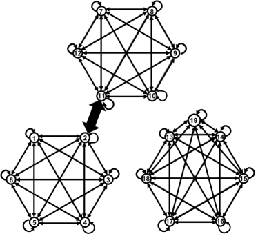
Figure 7: Channel described in Example 2. It consists of three complete graphs, and some additional edges. The thick solid arrow into node $y=11$ represents multiple edges connecting all the nodes in the set $\{1,2,3,4,5,6\}$ to node $11$. Similarly, all the nodes in the set $\{7,8,9,10,11,12\}$ are connected to node $2$.

[t] For any $\mathcal{Y}_{n}\subseteq\mathscr{Y}^{n}$, we define the uncertainty function $m_{\mathscr{Y}}(\mathcal{Y}_{n})$ in terms of cardinality

$$m_{\mathscr{Y}}(\mathcal{Y}_{n})=\frac{|\mathcal{Y}_{n}|}{|\mathscr{Y}^{n}|}.$$ (237)

Note that for all $n\in\mathbb{Z}_{>0}$, we have $m_{\mathscr{Y}}(\mathscr{Y}^{n})=1$.

It is easy to show that $m_{\mathscr{Y}}(.)$ satisfies Assumption 1. Namely, for $n=1$, we have that for all $\mathcal{Y}\subseteq\mathscr{Y}$,

$$m_{\mathscr{Y}}(\mathcal{Y})=\frac{|\mathcal{Y}|}{|\mathscr{Y}|}.$$ (238)

Let $\mathcal{Y}_{n}=\mathcal{Y}(1)\times\mathcal{Y}(2)\ldots\times\mathcal{Y}(n)$, where $\mathcal{Y}(i)\subseteq\mathscr{Y}$. Then, we have

$$\begin{split}&m_{\mathscr{Y}}(\mathcal{Y}_{n})\\ &=m_{\mathscr{Y}}(\mathcal{Y}(1)\times\mathcal{Y}(2)\ldots\times\mathcal{Y}(n)),\\ &=\frac{|\mathcal{Y}(1)\times\mathcal{Y}(2)\ldots\times\mathcal{Y}(n)|}{|\mathscr{Y}^{n}|},\\ &\stackrel{{\scriptstyle(a)}}{{=}}\frac{|\mathcal{Y}(1)|}{|\mathscr{Y}|}\frac{|\mathcal{Y}(2)|}{|\mathscr{Y}|}\ldots\frac{|\mathcal{Y}(n)|}{|\mathscr{Y}|},\\ &\stackrel{{\scriptstyle(b)}}{{=}}m_{\mathscr{Y}}(\mathcal{Y}(1))m_{\mathscr{Y}}(\mathcal{Y}(2))\ldots m_{\mathscr{Y}}(\mathcal{Y}(n)),\end{split}$$ (239)

where $(a)$ follows from the fact that for any two sets $\mathscr{S}_{1}$ and $\mathscr{S}_{2}$, $|\mathscr{S}_{1}\times\mathscr{S}_{2}|=|\mathscr{S}_{1}||\mathscr{S}_{2}|$, and $(b)$ follows from (238). It follows that $m_{\mathscr{Y}}(.)$ satisfies Assumption 1.

A similar argument shows that $m_{\mathscr{Y}}(.)$ also satisfies Assumption 2. Namely, let $\mathcal{Y}_{n}=\mathcal{Y}(1)\cup\mathcal{Y}(2)\ldots\cup\mathcal{Y}(n)$, where $\mathcal{Y}(i)\in\mathscr{Y}$. Then, we have

$$\begin{split}&m_{\mathscr{Y}}(\mathcal{Y}_{n})\\ &=m_{\mathscr{Y}}(\mathcal{Y}(1)\cup\mathcal{Y}(2)\ldots\cup\mathcal{Y}(n)),\\ &=\frac{|\mathcal{Y}(1)\cup\mathcal{Y}(2)\ldots\cup\mathcal{Y}(n)|}{|\mathscr{Y}|},\\ &\stackrel{{\scriptstyle(a)}}{{\leq}}\frac{|\mathcal{Y}(1)|}{|\mathscr{Y}|}+\frac{|\mathcal{Y}(2)|}{|\mathscr{Y}|}+\ldots+\frac{|\mathcal{Y}(n)|}{|\mathscr{Y}|},\\ &\stackrel{{\scriptstyle(b)}}{{=}}m_{\mathscr{Y}}(\mathcal{Y}(1))+m_{\mathscr{Y}}(\mathcal{Y}(2))+\ldots+m_{\mathscr{Y}}(\mathcal{Y}(n)),\end{split}$$ (240)

where $(a)$ follows from the fact that for any two sets $\mathscr{S}_{1}$ and $\mathscr{S}_{2}$, $|\mathscr{S}_{1}\cup\mathscr{S}_{2}|\leq|\mathscr{S}_{1}|+|\mathscr{S}_{2}|$, and $(b)$ follows from (238). It follows that $m_{\mathscr{Y}}(.)$ satisfies Assumption 2.

We now compute the capacity $C_{N}(\{\delta_{n}\})^{*}$ for $\delta_{1}=2/9$ and for all $n>1$ $\delta_{n}=(7/342)^{n}$.

Since $V_{N}$ contains seven elements, we have that $m_{\mathscr{Y}}(V_{N})=7/19$, and $\delta_{1}<m_{\mathscr{Y}}(V_{N})$. Consider an UV $\bar{X}$ representing a one-dimensional codebook such that

$$\llbracket\bar{X}\rrbracket=\{1,7,13\}.$$ (241)

It follows that the corresponding output UV $\bar{Y}$ is such that

$$\llbracket\bar{Y}\rrbracket=\{1,2,3,\ldots,18,19\}.$$ (242)

Letting $\bar{\delta}=1/6$, we have that $\bar{\delta}/|\llbracket X\rrbracket|=1/18$ and the overlap family

$$\llbracket\bar{Y}|\bar{X}\rrbracket^{*}_{1/18}=\{\mathscr{S}_{1},\mathscr{S}_{2}\},$$ (243)

where

$$\mathscr{S}_{1}=\cup_{x\in\{1,7\}}N(x),$$ (244)

$$\mathscr{S}_{2}=\cup_{x\in\{13\}}N(x).$$ (245)

We now show that $\bar{X}$ satisfies the sufficient conditions in Theorem 12. First, we note that for all $x\in\{2,3,4,5,6,8,9,10,11,12\}$, we have that $\llbracket\bar{Y}|x\rrbracket\subseteq\mathscr{S}_{1}$, and for all $x\in\{14,15,16,17,18,19\}$, we have $\llbracket\bar{Y}|x\rrbracket\subseteq\mathscr{S}_{2}$. It follows that for all $x\in\mathscr{X}\setminus\llbracket\bar{X}\rrbracket=\{2,3,4,5,6,8,9,10,11,12,14,15,16,17,18,19\}$, the uncertainity region $\llbracket\bar{Y}|x\rrbracket\subseteq\mathscr{S}$, where $\mathscr{S}\in\llbracket\bar{Y}|\bar{X}\rrbracket^{*}_{\bar{\delta}/|\llbracket\bar{X}\rrbracket|}$. Second, we have that

$$\bar{\delta}(1+1/|\llbracket\bar{X}\rrbracket|)=2/9\leq\delta_{1}/m_{\mathscr{Y}}(\llbracket\bar{Y}\rrbracket).$$ (246)

Third, we note that $\bar{\delta}=1/6$,

$$\bar{\delta}m_{\mathscr{Y}}(V_{N})/|\llbracket\bar{X}\rrbracket|=7/342.$$ (247)

It follows that for all $n>1$, we have that $\delta_{n}\leq(\bar{\delta}m_{\mathscr{Y}}(V_{N})/|\llbracket\bar{X}\rrbracket|)^{n}$.

Since all the sufficient conditions in Theorem 12 are satisfied, we have

$$C_{N}(\{\delta_{n}\})^{*}=\log_{2}|\llbracket\bar{Y}|\bar{X}\rrbracket^{*}_{1/18}|=1.$$ (248)

Example 3.

We now consider the same channel as in Example 2, shown in Figure 7, and we compute the capacity $C_{N}^{0*}$. We consider the one-dimensional codebook $\bar{X}$ in (241), and the corresponding output UV $\bar{Y}$ in (242). Then, we have

$$\llbracket\bar{Y}|\bar{X}\rrbracket^{*}_{0}=\{\mathscr{S}_{1},\mathscr{S}_{2}\},$$ (249)

where

$$\mathscr{S}_{1}=\cup_{x\in\{1,7\}}N(x),$$ (250)

$$\mathscr{S}_{2}=\cup_{x\in\{13\}}N(x).$$ (251)

We now show that $\bar{X}$ satisfies the sufficient conditions in Corollary 12.1. We note that for all $x\in\{2,3,4,5,6,8,9,10,11,12\}$, we have that $\llbracket\bar{Y}|x\rrbracket\subseteq\mathscr{S}_{1}$, and for all $x\in\{14,15,16,17,18,19\}$, we have $\llbracket\bar{Y}|x\rrbracket\subseteq\mathscr{S}_{2}$. It follows that for all $x\in\mathscr{X}\setminus\llbracket\bar{X}\rrbracket=\{2,3,4,5,6,8,9,10,11,12,14,15,16,17,18,19\}$, the uncertainity region $\llbracket\bar{Y}|x\rrbracket\subseteq\mathscr{S}$, where $\mathscr{S}\in\llbracket\bar{Y}|\bar{X}\rrbracket^{*}_{0}$.

Since all the sufficient conditions in Corollary 12.1 are satisfied, we have

$$C_{N}^{0*}=\log_{2}|\llbracket\bar{Y}|\bar{X}\rrbracket^{*}_{0}|=1.$$ (252)

Example 4.

We now consider the same channel as in Example 2, shown in Figure 7, and we compute the capacity $C_{N}(\{\delta_{n}\})_{*}$ for $\delta_{1}=(2/6)^{3}$ and for all $n>1$ $\delta_{n}=(2/6)^{3}((7/19)^{3}3)^{n-1}$.

For any $\mathcal{Y}_{n}\subseteq\mathscr{Y}^{n}$, we define the uncertainty function $m_{\mathscr{Y}}(\mathcal{Y}_{n})$ in terms of cardinality

$$m_{\mathscr{Y}}(\mathcal{Y}_{n})=\bigg{(}\frac{|\mathcal{Y}_{n}|}{|\mathscr{Y}^{n}|}\bigg{)}^{3}.$$ (253)

Note that for all $n\in\mathbb{Z}_{>0}$, we have $m_{\mathscr{Y}}(\mathscr{Y}^{n})=1$. It is easy to show that $m_{\mathscr{Y}}(.)$ satisfies Assumption 1. For $n=1$, we have that for all $\mathcal{Y}\subseteq\mathscr{Y}$,

$$m_{\mathscr{Y}}(\mathcal{Y})=\bigg{(}\frac{|\mathcal{Y}|}{|\mathscr{Y}|}\bigg{)}^{3}.$$ (254)

Let $\mathcal{Y}_{n}=\mathcal{Y}(1)\times\mathcal{Y}(2)\ldots\times\mathcal{Y}(n)$, where $\mathcal{Y}(i)\in\mathscr{Y}$. Then, we have

$$\begin{split}&m_{\mathscr{Y}}(\mathcal{Y}_{n})\\ &=m_{\mathscr{Y}}(\mathcal{Y}(1)\times\mathcal{Y}(2)\ldots\times\mathcal{Y}(n)),\\ &=\bigg{(}\frac{|\mathcal{Y}(1)\times\mathcal{Y}(2)\ldots\times\mathcal{Y}(n)|}{|\mathscr{Y}^{n}|}\bigg{)}^{3},\\ &\stackrel{{\scriptstyle(a)}}{{=}}\bigg{(}\frac{|\mathcal{Y}(1)|}{|\mathscr{Y}|}\bigg{)}^{3}\bigg{(}\frac{|\mathcal{Y}(2)|}{|\mathscr{Y}|}\bigg{)}^{3}\ldots\bigg{(}\frac{|\mathcal{Y}(n)|}{|\mathscr{Y}|}\bigg{)}^{3},\\ &\stackrel{{\scriptstyle(b)}}{{=}}m_{\mathscr{Y}}(\mathcal{Y}(1))m_{\mathscr{Y}}(\mathcal{Y}(2))\ldots m_{\mathscr{Y}}(\mathcal{Y}(n)),\end{split}$$ (255)

where $(a)$ follows from the fact that for any two sets $\mathscr{S}_{1}$ and $\mathscr{S}_{2}$, $|\mathscr{S}_{1}\times\mathscr{S}_{2}|=|\mathscr{S}_{1}||\mathscr{S}_{2}|$, and $(b)$ follows from (254). It follows that $m_{\mathscr{Y}}(.)$ satisfies Assumption 1.

Since $m_{\mathscr{Y}}(V_{N})=(7/19)^{3}$, we have $\delta_{1}<m_{\mathscr{Y}}(V_{N})$. We consider an UV $\bar{X}$ representing a one-dimensional codebook, a corresponding output UV $\bar{Y}$, and $\bar{\delta}=(2/6)^{3}$, so that

$$\llbracket\bar{X}\rrbracket=\{1,7,13\},$$ (256)

$$\llbracket\bar{Y}\rrbracket=\{1,2,\ldots,19\},$$ (257)

$$\llbracket\bar{Y}|\bar{X}\rrbracket^{*}_{1/81}=\{\mathscr{S}_{1},\mathscr{S}_{2},\mathscr{S}_{3}\},$$ (258)

where

$$\mathscr{S}_{1}=\cup_{x\in\{1\}}N(x),$$ (259)

$$\mathscr{S}_{2}=\cup_{x\in\{7\}}N(x),$$ (260)

$$\mathscr{S}_{3}=\cup_{x\in\{13\}}N(x).$$ (261)

Since $\bar{\delta}=\delta_{1}=(2/6)^{3}$, we have

$$\hat{\delta}=\max_{\mathscr{S}\in\llbracket\bar{Y}|\bar{X}\rrbracket^{*}_{\bar{\delta}/|\llbracket\bar{X}\rrbracket|}}\frac{m_{\mathscr{Y}}(\mathscr{S})}{m_{\mathscr{Y}}(\llbracket\bar{Y}\rrbracket)}=\bigg{(}\frac{7}{19}\bigg{)}^{3}.$$ (262)

It follows that for all $n>1$, we have $\delta_{n}\geq\bar{\delta}(\hat{\delta}|\llbracket\bar{X}\rrbracket|)^{n-1}$ and all the sufficient conditions in Theorem 13 are satisfied, so that

$$C_{N}(\{\delta_{n}\})_{*}=\log_{2}|\llbracket\bar{Y}|\bar{X}\rrbracket^{*}_{1/81}|=\log_{2}(3).$$ (263)

Example 5.

We again consider the same channel and the same uncertainty function as in Example 4, shown in Figure 7 and (253), respectively. We compute the capacity $C_{N}(\{\downarrow 0\})_{*}$. Consider an UV $X^{*}$ representing a one-dimensional codebook such that

$$\llbracket X^{*}\rrbracket=\{1,7,13\}.$$ (264)

It follows that the corresponding output UV $Y^{*}$ is such that

$$\llbracket Y^{*}\rrbracket=\{1,2,3\ldots 19\}.$$ (265)

Letting $\delta^{*}=(2/6)^{3}$, we have that $\delta^{*}/|\llbracket X^{*}\rrbracket|=1/81$ and the overlap family is

$$\llbracket Y^{*}|X^{*}\rrbracket^{*}_{\delta^{*}/|\llbracket X^{*}\rrbracket|=1/81}=\{\mathscr{S}_{1},\mathscr{S}_{2},\mathscr{S}_{3}\},$$ (266)

where

$$\mathscr{S}_{1}=\cup_{x\in\{1\}}N(x),$$ (267)

$$\mathscr{S}_{2}=\cup_{x\in\{7\}}N(x),$$ (268)

$$\mathscr{S}_{3}=\cup_{x\in\{13\}}N(x).$$ (269)

Since $V_{N}$ contains seven elements, we have that $m_{\mathscr{Y}}(V_{N})=(7/19)^{3}$, and $\delta^{*}<m_{\mathscr{Y}}(V_{N})$. Also, we have that

$$\hat{\delta}_{*}=\max_{\mathscr{S}\in\llbracket{Y}^{*}|{X}^{*}\rrbracket^{*}_{{\delta}^{*}/|\llbracket{X}^{*}\rrbracket|}}\frac{m_{\mathscr{Y}}(\mathscr{S})}{m_{\mathscr{Y}}(\llbracket{Y}^{*}\rrbracket)}=\bigg{(}\frac{7}{19}\bigg{)}^{3}.$$ (270)

It follows that $\hat{\delta}_{*}|\llbracket X^{*}\rrbracket|<1$.

Since all the sufficient conditions in Theorem 14 are satisfied, we have

$${C}_{N}(\{\downarrow 0\})_{*}=\log_{2}|\llbracket\bar{Y}|\bar{X}\rrbracket^{*}_{2/18}|=\log_{2}(3).$$ (271)

VIII-A Discussion

The results in our examples show that for the channel presented in Figure 7, and the uncertainty function (237), there exists a vanishing sequence $\delta_{1}=2/9,\{\delta_{n}\}_{2}^{\infty}=\{(7/342)^{n}\}$ such that

$$C_{N}^{0*}=C_{N}(\{\delta_{n}\})^{*}.$$ (272)

For the same channel and uncertainty function, there is another vanishing sequence $\delta_{1}=4/9,\{\delta_{n}\}_{2}^{\infty}=\{(14/342)^{n}\}$, such that

$$C_{N}^{0*}<C_{N}(\{\delta_{n}\})^{*}.$$ (273)

On the other hand, for the same channel using the uncertainty function (253), there exists a vanishing sequence $\delta_{1}=(2/6)^{3},\{\delta_{n}\}_{2}^{\infty}=\{(2/6)^{3}(3(7/19)^{3})^{n-1}\}$ such that

$$C_{N}(\{\delta_{n}\})_{*}={C}_{N}(\{\downarrow 0\})_{*}.$$ (274)

For the same channel and uncertainty function (253), there exists another sequence $\delta_{1}=(2/19)^{3},\{\delta_{n}\}_{2}^{\infty}=(2/19)^{3}(3(12/19)^{3})^{n-1}$ such that

$$C_{N}(\{\delta_{n}\})_{*}<{C}_{N}(\{\downarrow 0\})_{*}.$$ (275)

IX Applications

We now discuss some applications of the developed non-stochastic theory.

IX-A Error Correction in Adversarial Channels

Various adversarial channel models have been considered in the literature. A popular one considers a binary alphabet, and a codeword of length $n$ that is sent from the transmitter to the receiver. The channel can flip at most a fraction $0<\tau\leq 1$ of the $n$ symbols in an arbitrary fashion [20]. In this case, the input and output spaces are $\mathscr{X}^{n}=\mathscr{Y}^{n}=\{0,1\}^{n}$, and a codebook is $\mathcal{X}_{n}\subseteq\mathscr{X}^{n}$. Due to the constraint on the total number of bit flips, the channel is non-stationary and with memory. For any $x\in\mathscr{X}^{n}$, we can let the norm be the Hamming distance from the $n$-dimensional all zero vector representing the origin of the space, namely

$$\|x\|=H(x,\{0\}_{n})\leq n.$$ (276)

In this framework, for any transmitted codeword $x\in\mathcal{X}_{n}$, the set of possible received codewords is

$$S_{\tau n}(x)=\{y\in\mathscr{Y}^{n}:{H}(x,y)\leq\tau n\},$$ (277)

where $\tau n$ is the analogous of a noise range $\epsilon_{n}=\epsilon n$ in the non-stochastic channel model described in Section V.

For all $x_{1},x_{2}\in\mathcal{X}_{n}$, the equivocation region corresponds to $S_{\tau n}(x_{1})\cap S_{\tau n}(x_{2})$ and for any $\mathscr{S}\subseteq\mathscr{Y}^{n}$, we can define the uncertainty function

$$m_{\mathscr{Y}^{n}}(\mathscr{S})=\begin{cases}D(\mathscr{S})+1,\mbox{ if }\mathscr{S}\neq\emptyset,\\ 0,\mbox{ otherwise },\end{cases}$$ (278)

where $D$ indicates diameter, namely

$$D(\mathscr{S})=\max_{y_{1},y_{2}\in\mathscr{S}}H(y_{1},y_{2}).$$ (279)

With this definition, we have that

$$m_{\mathscr{Y}^{n}}(\mathscr{Y}^{n})=n+1.$$ (280)

For all $x_{1},x_{2}\in\mathcal{X}_{n}$, we let the error

$$e_{\tau n}(x_{1},x_{2})=\frac{m_{\mathscr{Y}^{n}}(S_{\tau n}(x_{1})\cap S_{\tau n}(x_{2}))}{n+1}.$$ (281)

As usual, we say that a codebook $\mathcal{X}_{n}$ is $(\tau n,\delta_{n})$-distinguishable if $e_{\tau n}(x_{1},x_{2})\leq{\delta_{n}}/{|\mathcal{X}_{n}|}$, and for all $n\in\mathbb{Z}_{>0}$ the $(\tau n,\delta_{n})$ capacity is

$$C^{\delta_{n}}_{\tau n}=\sup_{\mathcal{X}_{n}\in\mathscr{X}^{\delta_{n}}_{\tau n}}\log_{2}(|\mathcal{X}_{n}|),$$ (282)

where $\mathscr{X}^{\delta_{n}}_{\tau n}=\{\mathcal{X}_{n}:\mathcal{X}_{n}\mbox{ is }(\tau n,\delta_{n})\mbox{-distinguishable}\}$.

We now show that any $(\tau n,\delta_{n})$-distinguishable codebook $\mathcal{X}_{n}$ can be used to correct a certain number of bit flips. This number depends on how far apart any two codewords are, and a lower bound on this distance can be expressed in terms of the diameter of the equivocation set and of the amount of perturbation introduced by the channel, see Figure 8. The following theorem provides a lower bound on the Hamming distance $H(x_{1},x_{2})$ between any two codewords. The number of bit flips that can be corrected can then be computed using the well-known formula $\lfloor(H(x_{1},x_{2})-1)/2\rfloor$. Finally, we point out that non-stochastic, adversarial, error correcting codes are of interest and have been studied in the context of multi-label classification in machine learning [18], and to improve the robustness of neural networks to adversarial attacks [17].

Figure 8: The Hamming distance between any two overlapping codewords depends on the code parameters $\tau n$ and $\delta_{n}$.

Theorem 15.

Given a channel satisfying (277), if a codebook $\mathcal{X}_{n}$ is $(\tau n,\delta_{n})$-distinguishable, then for all $x_{1},x_{2}\in\mathcal{X}_{n}$, we have

$${H}(x_{1},x_{2})\geq\bigg{(}\frac{2\tau n}{n+1}-\frac{\delta_{n}}{|\mathcal{X}_{n}|}\bigg{)}(n+1)+1.$$ (283)

Proof.

Let $\mathcal{X}_{n}\in\mathscr{X}^{\delta}_{\tau n}$. Then, for all $x_{1},x_{2}\in\mathcal{X}_{n}$, we have

$$\begin{split}e_{\tau n}(x_{1},x_{2})&=\frac{m_{\mathscr{Y}^{n}}(S_{\tau n}(x_{1})\cap S_{\tau n}(x_{2}))}{n+1},\\ &\leq\frac{\delta_{n}}{|\mathcal{X}_{n}|}.\end{split}$$ (284)

First, we consider the case when

$$x_{1},x_{2}\in S_{\tau n}(x_{1})\cap S_{\tau n}(x_{2}).$$ (285)

Let $B(x_{1},x_{2})$ be the boundary of the equivocation set, namely

$$\begin{split}B(x_{1},x_{2})&=\{x\in S_{\tau n}(x_{1})\cap S_{\tau n}(x_{2})):\\ &\qquad\exists x^{\prime}\notin S_{\tau n}(x_{1})\cap S_{\tau n}(x_{2}))\mbox{ such that }\\ &\qquad H(x,x^{\prime})=1\}.\end{split}$$ (286)

By (285), there exist $A,B\in B(x_{1},x_{2})$ such that

$$H(A,B)=H(A,x_{1})+H(x_{1},x_{2})+H(x_{2},B).$$ (287)

Then, we have

$$\begin{split}H(A,B)&=H(A,x_{1})+H(x_{1},x_{2})+H(x_{2},B),\\ &\stackrel{{\scriptstyle(a)}}{{=}}2\tau n-2H(x_{1},x_{2})+H(x_{1},x_{2}),\\ &\stackrel{{\scriptstyle}}{{=}}2\tau n-H(x_{1},x_{2}),\end{split}$$ (288)

where $(a)$ follows from the fact that $A,B\in B(x_{1},x_{2})$, which implies

$$H(A,x_{1})=H(A,x_{2})-H(x_{1},x_{2})=\tau n-H(x_{1},x_{2}),$$ (289)

and

$$H(B,x_{2})=H(B,x_{1})-H(x_{1},x_{2})=\tau n-H(x_{1},x_{2}).$$ (290)

We now have that

$$\begin{split}H(x_{1},x_{2})&=2\tau n-H(A,B),\\ &\stackrel{{\scriptstyle(a)}}{{\geq}}2\tau n-D(S_{\tau n}(x_{1})\cap S_{\tau n}(x_{2})),\end{split}$$ (291)

where $(a)$ follows from the fact that using $A,B\in S_{\tau n}(x_{1})\cap S_{\tau n}(x_{2}))$, we have $H(A,B)\leq D(S_{\tau n}(x_{1})\cap S_{\tau n}(x_{2}))$.

Now, we consider the case when

$$x_{1},x_{2}\notin S_{\tau n}(x_{1})\cap S_{\tau n}(x_{2}).$$ (292)

In this case, we have

$$\begin{split}&H(x_{1},x_{2})\\ &\stackrel{{\scriptstyle}}{{\geq}}2\tau n-D(S_{\tau n}(x_{1})\cap S_{\tau n}(x_{2})).\\ \end{split}$$ (293)

The result now follows by combining (291), (293) and (284).

∎

IX-B Robustness of Neural Networks to Adversarial Attacks

Motivated by security considerations, the robustness of neural networks to adversarial examples has recently received great attention [16, 21, 22]. While different algorithms have been proposed to improve robustness [21, 22], studies quantifying the limits of robustness have been limited [16, 23]. We argue that the non-stochastic framework introduced in this paper can be a viable way to quantify robustness, and can be used as a baseline to evaluate the performance of different algorithmic solutions.

We follow the framework of [16] and consider a neural network trained to classify the incoming data among $L$ possible labels in the set $\mathscr{L}=\{1,2,\ldots,L\}$. Let $x_{0}\in\mathbb{R}^{d}$ denote an input data point consisting of a feature vector of $d$ dimensions. A neural network can be modelled using a classification function $f:\mathbb{R}^{d}\to\mathbb{R}^{L}$ whose $\ell$th component $f_{\ell}(\cdot)$ indicates the belief that a given data point is of label $\ell$. The network classifies each input data point $x_{0}$ as being of label

$$c(x_{0})=\mbox{argmax}_{\ell\in\{1,\ldots,L\}}f_{\ell}(x_{0}).$$ (294)

We let $\mathcal{D}(\ell)\subseteq\mathcal{D}$ denote the set of points in a data set $\mathcal{D}$ that are classified as being of label $\ell$, namely

$$\mathcal{D}(\ell)=\{x_{0}\in\mathcal{D}:c(x_{0})=\ell\}.$$ (295)

When the points in this set are subject to an $\epsilon$-attack, they become part of the perturbed input data set

$$\begin{split}S_{\epsilon}(\ell)&=\{x\in\mathbb{R}^{d}:\;\|x-x_{0}\|\leq\epsilon,x_{0}\in\mathcal{D}(\ell)\}.\end{split}$$ (296)

An $\epsilon$-attack on input point $x_{0}$ is successful if there exists a noise vector $e\in\mathbb{R}^{d}$ such that

$$c(x_{0})\neq c(x_{0}+e),\mbox{ and }\|e\|\leq\epsilon.$$ (297)

For any two labels $\ell_{1},\ell_{2}\in\{1,2,\ldots,L\}$, we let

$$\begin{split}\mathcal{P}_{\epsilon}(\ell_{1},\ell_{2})=&\{x\in S_{\epsilon}(\ell_{1}):\mbox{ either }c(x)=\ell_{1}\\ &\mbox{ or }c(x)=\ell_{2}\}.\end{split}$$ (298)

Then, $\mathcal{P}_{\epsilon}(\ell_{1},\ell_{2})\cap\mathcal{P}_{\epsilon}(\ell_{2},\ell_{1})$ represents the set of points in $\mathcal{S}_{\epsilon}(\ell_{1})$ and $\mathcal{S}_{\epsilon}(\ell_{2})$ that can lead to a successful $\epsilon$-attack.

For all $\ell_{1},\ell_{2}\in\{1,2,\ldots,L\}$, we let the error

$$e_{\epsilon}(\ell_{1},\ell_{2})=\frac{m_{\mathscr{L}}(\mathcal{P}_{\epsilon}(\ell_{1},\ell_{2})\cap\mathcal{P}_{\epsilon}(\ell_{2},\ell_{1}))}{m_{\mathscr{L}}(\mathscr{L})}.$$ (299)

Finally, we say that a subset of labels (viz. a codebook) $\mathcal{L}\subseteq{\mathscr{L}}$ is $(\epsilon,\delta)$-robust if for all $\ell_{1},\ell_{2}\in\mathcal{L}$, we have $e_{\epsilon}(\ell_{1},\ell_{2})\leq\delta/|\mathcal{L}|$. This implies that whenever a label in an $(\epsilon,\delta)$-robust codebook is assigned to any input point that is subject to an attack, this is the same as the label assigned to the same input in the absence of the attack, with confidence at least $1-\delta$.

We can then define the $(\epsilon,\delta)$- robust capacity of the neural network as the logarithm of the maximum number of labels that can be robustly classified with confidence $1-\delta$ in the presence of an $\epsilon$-attack, namely

$$C^{\delta}_{\epsilon}(\mathcal{D})=\sup_{\mathcal{L}\in\mathscr{L}^{\delta}_{\epsilon}(\mathcal{D})}\log_{2}(|\mathcal{L}|),$$ (300)

where $\mathscr{L}^{\delta}_{\epsilon}(\mathcal{D})=\{\mathcal{L}:\mathcal{L}\mbox{ is }(\epsilon,\delta)\mbox{-robust}\}$. This capacity represents the largest amount of information that the labeling task of the neural network can convey, at a given level of confidence, under a perturbation attack. This information is independent of whether the neural network classifies the input data correctly or not.

For $\epsilon=0$, for any two labels $\ell_{1},\ell_{2}\in\mathscr{L}$, we have that $\mathcal{D}(\ell_{1})=S_{\epsilon}(\ell_{1})$ and $\mathcal{P}_{\epsilon}(\ell_{1},\ell_{2})=\mathcal{D}(\ell_{1})$, which implies that

$$\mathcal{P}_{\epsilon}(\ell_{1},\ell_{2})\cap\mathcal{P}_{\epsilon}(\ell_{2},\ell_{1})=\emptyset,$$ (301)

and the capacity $C^{\delta}_{\epsilon}(\mathcal{D})=\log_{2}(L)$, regardless of the value of $\delta$. This means that in the absence an attack, the amount of information conveyed by the network is simply the logarithm of the number of labels it classifies the data into.

The framework described above has been studied in the special case of $\delta=0$ and for a single input data point $x_{0}$ in [16]. Our $(\epsilon,\delta)$- robust capacity generalizes the notion of robustness from a single point $x_{0}$ to the whole data set $\mathcal{D}$ and can quantify the overall robustness of a neural network.

IX-C Performance of Classification Systems

The non-stochastic $(N,\delta)$ capacity can also be used as a performance measure of classification systems operating on a given data set. Consider a system trained to classify the incoming data among $L$ possible labels in the set $\mathscr{L}=\{1,2,\ldots,L\}$. Let $x_{0}$ be an input data point, and $c(x_{0})$ be the label assigned by the neural network to $x_{0}$. For a given data set $\mathcal{D}$, let $N(\ell)\subseteq\{1,2,\ldots,L\}$ denote the subset of labels such that

$$\begin{split}N(\ell)=&\{\ell^{\prime}\in\mathscr{L}:\mbox{ there exists a data point }x_{0}\in\mathcal{D}\\ &\mbox{ such that }\mbox{the correct label of $x_{0}$ is $\ell$ and }\\ &c(x_{0})=\ell^{\prime}\}.\end{split}$$ (302)

If $\ell\in N(\ell)$, then there exists a data point that is correctly classified as $\ell$. If $\ell^{\prime}\in N(\ell)$ such that $\ell^{\prime}\neq\ell$, then there exists a data point that is incorrectly classified as $\ell^{\prime}$, and the correct label of this data point is $\ell$.

For any two labels $\ell_{1},\ell_{2}\in\mathscr{L}$, we have the equivocation region $N(\ell_{1})\cap N(\ell_{2})$, and we let the error

$$e_{N}(\ell_{1},\ell_{2})=\frac{|N(\ell_{1})\cap N(\ell_{2})|}{|\mathscr{L}|}.$$ (303)

We say that a subset of labels $\mathcal{L}\subseteq\mathscr{L}$ is $(N,\delta)$-classifiable if for all $\ell_{1},\ell_{2}\in\mathcal{L}$, we have $e_{N}(\ell_{1},\ell_{2})\leq\delta/|\mathcal{L}|$, and the $(N,\delta)$-capacity of the classification system is

$$C_{N}^{\delta}=\sup_{\mathcal{L}\in\mathscr{L}^{\delta}_{N}}\log_{2}(|\mathcal{L}|),$$ (304)

where $\mathscr{L}^{\delta}_{N}=\{\mathcal{L}:\mathcal{L}\mbox{ is }(N,\delta)\mbox{-classifiable}\}$. Given the set of labels, this capacity quantifies the amount of information that the classifier is able to extract from a given data set, in terms of the logarithm of the largest number of labels that can be identified with confidence greater than $1-\delta$. In contrast to the robust capacity described in Section IX-B, here the capacity refers to the ability of the network to perform the classification task correctly in the absence of an attack, rather than to its ability of performing classification consistently (but not necessarily correctly) in the presence of an attack.

X Conclusion

In this paper, we presented a non-stochastic theory of information that is based on a notion of information with worst-case confidence that is independent of stochastic modeling assumptions. Using the non-stochastic variables framework of Nair [5], we showed that the capacity of several channel models equals the largest amount of information conveyed by the transmitter to the receiver, with a given level of confidence. These results are the natural generalization of Nair’s ones, obtained in a zero-error framework, and provide an information-theoretic interpretation for the geometric problem of sphere packing with overlap, studied by Lim and Franceschetti [11]. More generally, they show that the path laid by Shannon can be extended to a non-stochastic setting, which is an idea that dates back to Kolmogorov [24].

Non-stochastic approaches to information, and their usage to quantify the performance of engineering systems have recently received attention in the context of estimation, control, security, communication over non-linear optical channels, and learning systems [12, 13, 14, 15, 16, 17, 18]. We hope that the theory developed here can be useful in some of these contexts. To this end, we pointed out some possible applications in the context of classification systems and communication over adversarial channels.

While refinements and extension of the theory are certainly of interest, further exploration of application domains is of paramount importance. There is evidence in the literature for the need of a non-stochastic approach to study the flow of information in complex systems, and there is a certain tradition in computer science and especially in the field of online learning to study various problems in both a stochastic and a non-stochastic setting [25, 26, 27, 28, 29]. Nevertheless, it seems that only a few isolated efforts have been made towards the formal development of a non-stochastic information theory. A wider involvement of the community in developing alternative, even competing, theories is certainly advisable to eventually fulfill the need of several application areas.

-A Proof of Lemma 1

Proof.

Let $(X,Y)\stackrel{{\scriptstyle a}}{{\leftrightarrow}}(\delta_{1},\delta_{2})$. Then,

$$\mathscr{A}(X;Y)\preceq\delta_{1},$$ (305)

$$\mathscr{A}(Y;X)\preceq\delta_{2}.$$ (306)

Let

$$\mathscr{S}_{1}=\bigg{\{}(y_{1},y_{2}):\frac{m_{\mathscr{X}}(\llbracket X|y_{1}\rrbracket\cap\llbracket X|y_{2}\rrbracket|)}{m_{\mathscr{X}}(\llbracket X\rrbracket)}=0\bigg{\}}.$$ (307)

Then, for all $(y_{1},y_{2})\in\mathscr{S}_{1}$, we have

$$\frac{m_{\mathscr{X}}(\llbracket X|y_{1}\rrbracket\cap\llbracket X|y_{2}\rrbracket|)}{m_{\mathscr{X}}(\llbracket X\rrbracket)}=0\leq\delta_{1}.$$ (308)

Also, if $(y_{1},y_{2})\in\mathscr{S}_{1}$, then

$$\frac{m_{\mathscr{X}}(\llbracket X|y_{1}\rrbracket\cap\llbracket X|y_{2}\rrbracket|)}{m_{\mathscr{X}}(\llbracket X\rrbracket)}\notin\mathscr{A}(X;Y),$$ (309)

and if $(y_{1},y_{2})\notin\mathscr{S}_{1}$, then using (8), we have

$$\frac{m_{\mathscr{X}}(\llbracket X|y_{1}\rrbracket\cap\llbracket X|y_{2}\rrbracket|)}{m_{\mathscr{X}}(\llbracket X\rrbracket)}\in\mathscr{A}(X;Y).$$ (310)

This along with (305) and (308) implies that (16) follows.

Likewise, let

$$\mathscr{S}_{2}=\bigg{\{}(x_{1},x_{2}):\frac{m_{\mathscr{Y}}(\llbracket Y|x_{1}\rrbracket\cap\llbracket Y|x_{2}\rrbracket|)}{m_{\mathscr{Y}}(\llbracket Y\rrbracket)}=0\bigg{\}}.$$ (311)

Then, for all $(x_{1},x_{2})\in\mathscr{S}_{2}$,

$$\frac{m_{\mathscr{Y}}(\llbracket Y|x_{1}\rrbracket\cap\llbracket Y|x_{2}\rrbracket|)}{m_{\mathscr{Y}}(\llbracket Y\rrbracket)}=0\leq\delta_{2}.$$ (312)

Also, if $(x_{1},x_{2})\in\mathscr{S}_{2}$, then

$$\frac{m_{\mathscr{Y}}(\llbracket Y|x_{1}\rrbracket\cap\llbracket Y|x_{2}\rrbracket|)}{m_{\mathscr{Y}}(\llbracket Y\rrbracket)}\notin\mathscr{A}(Y;X),$$ (313)

and if $(y_{1},y_{2})\notin\mathscr{S}_{2}$, then using (8), we have

$$\frac{m_{\mathscr{Y}}(\llbracket Y|x_{1}\rrbracket\cap\llbracket Y|x_{2}\rrbracket|)}{m_{\mathscr{Y}}(\llbracket Y\rrbracket)}\in\mathscr{A}(Y;X).$$ (314)

This along with (306) and (312) implies that (17) follows.

Now, we prove the opposite direction of the statement. Given that for all $y_{1},y_{2}\in\llbracket Y\rrbracket$, we have

$$\frac{m_{\mathscr{X}}(\llbracket X|y_{1}\rrbracket\cap\llbracket X|y_{2}\rrbracket|)}{m_{\mathscr{X}}(\llbracket X\rrbracket)}\leq\delta_{1},$$ (315)

and for all $x_{1},x_{2}\in\llbracket X\rrbracket$, we have

$$\frac{m_{\mathscr{Y}}(\llbracket Y|x_{1}\rrbracket\cap\llbracket Y|x_{2}\rrbracket|)}{m_{\mathscr{Y}}(\llbracket Y\rrbracket)}\leq\delta_{2}.$$ (316)

Then, using the definition of $\mathscr{A}(X;Y)$ and $\mathscr{A}(Y;X)$, we have

$$\mathscr{A}(X;Y)\preceq\delta_{1},$$ (317)

$$\mathscr{A}(Y;X)\preceq\delta_{2}.$$ (318)

The statement of the lemma follows. ∎

-B Proof of Theorem 9

Proof.

We will show (133). Then, using Lemma 6 in Appendix -D, (134) follows using the same argument as in the proof of Theorem 8.

We proceed in three steps. First, we show that for all $n>0$, there exists an UV $X(1:n)$ and $\tilde{\delta}\leq\delta_{n}/m_{\mathscr{Y}}(\llbracket Y(1:n)\rrbracket)$ such that ${X}(1:n)\in\mathscr{F}_{\tilde{\delta}}(n)$, which implies $\mathscr{F}_{\tilde{\delta}}(n)$ is not empty, so that the supremum is well defined. Second, for all $n>0$, and $X(1:n)$ and $\tilde{\delta}$ such that

$$X(1:n)\in\mathscr{F}_{\tilde{\delta}}(n),$$ (319)

and

$$\tilde{\delta}\leq\delta_{n}/m_{\mathscr{Y}}(\llbracket Y(1:n)\rrbracket),$$ (320)

we show that

$$\frac{I_{\tilde{\delta}/|\llbracket X(1:n)\rrbracket|}(Y(1:n);X(1:n))}{n}\leq R_{\delta_{n}}.$$

Finally, for all $n>0$, we show the existence of $X(1:n)\in\mathscr{F}_{\tilde{\delta}}(n)$ and $\tilde{\delta}\leq\delta_{n}/m_{\mathscr{Y}}(\llbracket Y(1:n)\rrbracket)$ such that

$$\frac{I_{\tilde{\delta}/|\llbracket X(1:n)\rrbracket|}(Y(1:n);X(1:n))}{n}=R_{\delta_{n}}.$$ (321)

Let us begin with the first step. Consider a point $x(1:n)\in\mathscr{X}^{n}$. Let $X(1:n)$ be a UV such that

$$\llbracket X(1:n)\rrbracket=\{x(1:n)\}.$$ (322)

Then, we have that the marginal range of the UV $Y(1:n)$ corresponding to the received variable is

$$\llbracket Y(1:n)\rrbracket=\llbracket Y(1:n)|x(1:n)\rrbracket,$$ (323)

and therefore for all $y(1:n)\in\llbracket Y(1:n)\rrbracket$, we have

$$\llbracket X(1:n)|y(1:n)\rrbracket=\{x(1:n)\}.$$ (324)

Using Definition 2 and (322), we have that

$$\mathscr{A}(Y(1:n);X(1:n))=\emptyset,$$ (325)

because $\llbracket X(1:n)\rrbracket$ consists of a single point, and therefore the set in (11) is empty.

On the other hand, using Definition 2 and (324), we have

$$\mathscr{A}(X(1:n);Y(1:n))=\begin{cases}\{1\}\mbox{ if }\exists y_{1}(1:n),y_{2}(1:n)\\ \qquad\qquad\in\llbracket Y(1:n)\rrbracket,\\ \emptyset\quad\mbox{ otherwise}.\end{cases}$$ (326)

Using (325) and since $\mathscr{A}\preceq\delta$ holds for $\mathscr{A}=\emptyset$, we have

$$\mathscr{A}(Y(1:n);X(1:n))\preceq\delta_{n}/(|\llbracket X(1:n)\rrbracket|m_{\mathscr{Y}}(\llbracket Y(1:n)\rrbracket)).$$ (327)

Similarly, using (326) we have

$$\mathscr{A}(X(1:n);Y(1:n))\preceq 1.$$ (328)

Now, combining (327) and (328), we have

$$(X(1:n),Y(1:n))\stackrel{{\scriptstyle a}}{{\leftrightarrow}}(1,\delta_{n}/(|\llbracket X(1:n)\rrbracket|m_{\mathscr{Y}}(\llbracket Y(1:n)\rrbracket))).$$ (329)

Letting $\tilde{\delta}=\delta_{n}/m_{\mathscr{Y}}(\llbracket Y(1:n)\rrbracket)$, this implies that $X(1:n)\in\mathscr{F}_{\tilde{\delta}}(n)$ and the first step of the proof is complete.

To prove the second step, we define

$$\begin{split}\mathscr{G}(n)=&\bigg{\{}X(1:n):\llbracket X(1:n)\rrbracket\subseteq\mathscr{X}^{n},\\ &\exists\tilde{\delta}\leq\delta_{n}/m_{\mathscr{Y}}(\llbracket Y(1:n)\rrbracket)\mbox{ such that }\\ &\forall\mathscr{S}_{1},\mathscr{S}_{2}\in\llbracket Y(1:n)|X(1:n)\rrbracket,\\ &\frac{m_{\mathscr{Y}}(\mathscr{S}_{1}\cap\mathscr{S}_{2})}{m_{\mathscr{Y}}(\llbracket Y(1:n)\rrbracket)}\leq\frac{\tilde{\delta}}{|\llbracket X(1:n)\rrbracket|}\bigg{\}},\end{split}$$ (330)

which is a larger set than the one containing all UVs $X(1:n)$ that are $(1,\tilde{\delta}/|\llbracket X(1:n)\rrbracket|)$ associated to $Y(1:n)$. Similar to (76), it can be shown that

$$X(1:n)\in\mathscr{G}(n)\implies\mathcal{X}(1:n)\in\mathscr{X}_{N}^{\delta_{n}}(n)$$ (331)

Consider now a pair $X(1:n)$ and $\tilde{\delta}$ such that $\tilde{\delta}\leq\delta_{n}/m_{\mathscr{Y}}(\llbracket Y(1:n)\rrbracket)$, and

$$X(1:n)\in\mathscr{F}_{\tilde{\delta}}(n).$$ (332)

If $(X(1:n),Y(1:n))\stackrel{{\scriptstyle d}}{{\leftrightarrow}}(0,\tilde{\delta}/|\llbracket X(1:n)\rrbracket|)$, then using Lemma 3 in Appendix -D, there exist UVs $\bar{X}(1:n)$ and $\bar{Y}(1:n)$ and $\bar{\delta}\leq\delta_{n}/m_{\mathscr{Y}}(\llbracket\bar{Y}(1:n)\rrbracket)$ such that

$$(\bar{X}(1:n),\bar{Y}(1:n))\stackrel{{\scriptstyle a}}{{\leftrightarrow}}(1,\bar{\delta}/|\llbracket\bar{X}(1:n)\rrbracket|),$$ (333)

and

$$\begin{split}&|\llbracket Y(1:n)|X(1:n)\rrbracket^{*}_{\tilde{\delta}/|\llbracket X(1:n)\rrbracket|}|\\ &=|\llbracket\bar{Y}(1:n)|\bar{X}(1:n)\rrbracket_{\bar{\delta}/|\llbracket\bar{X}(1:n)\rrbracket|}^{*}|.\end{split}$$ (334)

On the other hand, if $(X(1:n),{Y}(1:n))\stackrel{{\scriptstyle a}}{{\leftrightarrow}}(1,\tilde{\delta}/|\llbracket{X}(1:n)\rrbracket|)$, then (333) and (334) also trivially hold. It then follows that (333) and (334) hold for all $X(1:n)\in\mathscr{F}_{\tilde{\delta}}(n)$. We now have

$$\begin{split}&I_{\tilde{\delta}/|\llbracket X(1:n)\rrbracket|}(Y(1:n);X(1:n))\\ &=\log(|\llbracket Y(1:n)|X(1:n)\rrbracket_{\tilde{\delta}/|\llbracket X(1:n)\rrbracket|}^{*}|)\\ &\stackrel{{\scriptstyle(a)}}{{=}}\log(|\llbracket\bar{Y}(1:n)|\bar{X}(1:n)\rrbracket_{\bar{\delta}/|\llbracket\bar{X}(1:n)\rrbracket|}^{*}|)\\ &\stackrel{{\scriptstyle(b)}}{{\leq}}\log(|\llbracket\bar{X}(1:n)\rrbracket|),\\ &\stackrel{{\scriptstyle(c)}}{{=}}\log(|\bar{\mathcal{X}}(1:n)|),\\ &\stackrel{{\scriptstyle(d)}}{{\leq}}nR_{\delta_{n}},\end{split}$$ (335)

where $(a)$ follows from (333) and (334), $(b)$ follows from Lemma 5 in Appendix -D since $\bar{\delta}\leq\delta_{n}/m_{\mathscr{Y}}(\llbracket\bar{Y}(1:n)\rrbracket)<m_{\mathscr{Y}}(V^{n}_{N})/m_{\mathscr{Y}}(\llbracket\bar{Y}(1:n)\rrbracket)$, $(c)$ follows by defining the codebook $\bar{\mathcal{X}}(1:n)$ corresponding to the UV $\llbracket\bar{X}(1:n)\rrbracket$ , and $(d)$ follows from the fact that using (333) and Lemma 1, we have $\bar{X}(1:n)\in\mathcal{G}(n)$, which implies by (331) that $\bar{\mathcal{X}}(1:n)\in\mathscr{X}_{N}^{\delta_{n}}(n)$.

For any $n\in\mathbb{Z}_{>0}$, let

$$\mathcal{X}_{n}^{*}=\mbox{argsup}_{\mathcal{X}_{n}\in\mathscr{X}^{\delta_{n}}_{N}(n)}\frac{\log(|\mathcal{X}_{n}|)}{n},$$ (336)

which achieves the rate $R_{\delta_{n}}$. Let ${{X}}^{*}$ be the UV whose marginal range corresponds to the codebook $\mathcal{{X}}_{n}^{*}$. It follows that for all $\mathscr{S}_{1},\mathscr{S}_{1}\in\llbracket Y^{*}|{X}^{*}\rrbracket$, we have

$$\frac{m_{\mathscr{Y}}(\mathscr{S}_{1}\cap\mathscr{S}_{1})}{m_{\mathscr{Y}}(\mathscr{Y}^{n})}\leq\frac{\delta_{n}}{|\llbracket{X}^{*}\rrbracket|},$$ (337)

which implies using the fact that $m_{\mathscr{Y}}(\mathscr{Y}^{n})=1$,

$$\frac{m_{\mathscr{Y}}(\mathscr{S}_{1}\cap\mathscr{S}_{1})}{m_{\mathscr{Y}}(\llbracket Y^{*}\rrbracket)}\leq\frac{\delta_{n}}{(|\llbracket{X}^{*}\rrbracket|m_{\mathscr{Y}}(\llbracket Y^{*}\rrbracket))}.$$ (338)

Letting $\delta^{*}=\delta_{n}/m_{\mathscr{Y}}(\llbracket Y^{*}\rrbracket)$, and using Lemma 1, we have that $(X^{*},{Y}^{*})\stackrel{{\scriptstyle a}}{{\leftrightarrow}}(1,\delta^{*}/|\llbracket X^{*}\rrbracket|)$, which implies

$${X}^{*}\in\cup_{\tilde{\delta}\leq\delta_{n}/m_{\mathscr{Y}}(\llbracket Y^{*}\rrbracket)}\mathscr{F}_{\tilde{\delta}}(n),$$ (339)

and (133) follows. ∎

-C Proof of Lemma 2

Proof.

Let us begin with part $1)$. We have

$$\begin{split}&\llbracket Y(1:n)\rrbracket\\ &\stackrel{{\scriptstyle}}{{=}}\cup_{x(1:n)\in\llbracket X(1:n)\rrbracket}\llbracket Y(1:n)|x(1:n)\rrbracket,\\ &\stackrel{{\scriptstyle(a)}}{{=}}\cup_{x(1:n)\in\llbracket X(1:n)\rrbracket}\llbracket Y(1)|x(1)\rrbracket\times\ldots\llbracket Y(n)|x(n)\rrbracket,\\ &\stackrel{{\scriptstyle(b)}}{{=}}\cup_{x(1)\in\llbracket X(1)\rrbracket}\llbracket Y(1)|x(1)\rrbracket\times\\ &\quad\ldots\times\cup_{x(n)\in\llbracket X(n)\rrbracket}\llbracket Y(n)|x(n)\rrbracket,\\ &=\llbracket Y(1)\rrbracket\times\llbracket Y(2)\rrbracket\times\ldots\times\llbracket Y(n)\rrbracket,\\ \end{split}$$ (340)

where $(a)$ follows from (143), and $(b)$ follows from (142). Now, we have

$$\begin{split}\bigcup_{\mathscr{S}\in\prod_{i=1}^{n}\llbracket Y(i)|X(i)\rrbracket^{*}_{\delta}}\mathscr{S}&\stackrel{{\scriptstyle(a)}}{{=}}\prod_{i=1}^{n}(\bigcup_{\mathscr{S}\in\llbracket Y(i)|X(i)\rrbracket^{*}_{\delta}}\mathscr{S}),\\ &\stackrel{{\scriptstyle(b)}}{{=}}\prod_{i=1}^{n}\llbracket Y(i)\rrbracket,\\ &\stackrel{{\scriptstyle(c)}}{{=}}\llbracket Y(1:n)\rrbracket,\end{split}$$ (341)

where $(a)$ follows from the fact that the cartesian product is distributive over union, namely

$$\cup_{(i,j)\in I\times J}A_{i}\times B_{j}=(\cup_{i\in I}A_{i})\times(\cup_{j\in J}B_{j}),$$ (342)

$(b)$ follows from the fact that for all $1\leq i\leq n$, $\llbracket Y(i)|X(i)\rrbracket^{*}_{\delta}$ is a covering of $\llbracket Y(i)\rrbracket$ by Definition 6, and $(c)$ follows from (340). Hence, part $1)$ follows.

Now, we prove part $2)$. Here, we will first show that for all $\mathscr{S}\in\prod_{i=1}^{n}\llbracket Y(i)|X(i)\rrbracket^{*}_{\delta}$, we have that $\mathscr{S}$ is $\delta^{n}$-connected. Second, we will show that $\mathscr{S}$ contains at least one singly $\delta^{n}$-connected set.

Let us begin with the first step of part $2)$. Consider a set $\mathscr{S}\in\prod_{i=1}^{n}\llbracket Y(i)|X(i)\rrbracket^{*}_{\delta}$. Then, there exists a sequence $\{\mathscr{S}_{i}\}_{i=1}^{n}$ such that

$$\mathscr{S}=\mathscr{S}_{1}\times\mathscr{S}_{2}\times\ldots\times\mathscr{S}_{n},$$ (343)

and for all $1\leq i\leq n$,

$$\mathscr{S}_{i}\in\llbracket Y(i)|X(i)\rrbracket^{*}_{\delta}.$$ (344)

Now, consider two points $y_{1}(1:n),y_{2}(1:n)\in\mathscr{S}$. Then, using (143), (340) and (343), for all $1\leq i\leq n$, we have that

$$y_{1}(i),y_{2}(i)\in\mathscr{S}_{i}.$$ (345)

Also, since $\mathscr{S}_{i}$ is $\delta$-connected using (344) and Property 1 of Definition 6, we have

$$y_{1}(i)\stackrel{{\scriptstyle\delta}}{{\leftrightsquigarrow}}y_{2}(i),$$ (346)

namely there exists a sequence $\{\llbracket Y(i)|x_{k}(i)\rrbracket\}_{k=1}^{N(i)}$ such that

$$y_{1}(i)\in\llbracket Y(i)|x_{1}(i)\rrbracket,y_{2}(i)\in\llbracket Y(i)|x_{N(i)}(i)\rrbracket,$$ (347)

and for all $1\leq k<N(i)$,

$$\frac{m_{\mathscr{Y}}(\llbracket Y(i)|x_{k}(i)\rrbracket\cap\llbracket Y(i)|x_{k+1}(i)\rrbracket)}{m_{\mathscr{Y}}(\llbracket Y(i)\rrbracket)}>\delta.$$ (348)

Without loss of generality, let

$$N(1)\leq N(2)\leq\ldots\leq N(n).$$ (349)

Now, consider the following sequence of conditional ranges

$$\begin{split}&\llbracket Y(1:n)|x_{1}(1),x_{1}(2)\ldots x_{1}(n)\rrbracket,\\ &\llbracket Y(1:n)|x_{2}(1),x_{2}(2)\ldots x_{2}(n)\rrbracket,\\ &\ldots\\ &\llbracket Y(1:n)|x_{N(1)}(1),x_{N(1)}(2)\ldots x_{N(1)}(n)\rrbracket,\\ &\llbracket Y(1:n)|x_{N(1)}(1),x_{N(1)+1}(2)\ldots x_{N(1)+1}(n)\rrbracket,\\ &\ldots\\ &\llbracket Y(1:n)|x_{N(1)}(1),x_{N(2)}(2)\ldots x_{N(n)}(n)\rrbracket.\\ \end{split}$$ (350)

In this sequence, for all $1\leq k<N(n)$, if $x_{k}(i)=x_{k+1}(i)$, then we have

$$\begin{split}&\frac{m_{\mathscr{Y}}(\llbracket Y(i)|x_{k}(i)\rrbracket\cap\llbracket Y(i)|x_{k+1}(i)\rrbracket)}{m_{\mathscr{Y}}(\llbracket Y(i)\rrbracket)}\\ &\stackrel{{\scriptstyle(a)}}{{=}}\frac{m_{\mathscr{Y}}(\llbracket Y(i)|x_{k}(i)\rrbracket)}{m_{\mathscr{Y}}(\llbracket Y(i)\rrbracket)},\\ &\stackrel{{\scriptstyle(b)}}{{>}}\frac{\delta}{m_{\mathscr{Y}}(\llbracket Y(i)\rrbracket)},\\ &\stackrel{{\scriptstyle(c)}}{{\geq}}\frac{\delta}{m_{\mathscr{Y}}(\mathscr{Y})},\\ &\stackrel{{\scriptstyle(d)}}{{>}}\delta,\end{split}$$ (351)

where $(a)$ follows from the fact that $x_{k}(i)=x_{k+1}(i)$, $(b)$ follows from (144), $(c)$ follows from the fact that $\llbracket Y(i)\rrbracket\subseteq\mathscr{Y}$ and (9) holds, and $(d)$ follows from the fact that $m_{\mathscr{Y}}(\mathscr{Y})=1$. Additionally, in the sequence (350), for all $1\leq k<N(n)$, if $x_{k}(i)\neq x_{k+1}(i)$, then we have that (348) holds. This along with (351) implies that for all $1\leq k<N(n)$, we have

$$\frac{m_{\mathscr{Y}}(\llbracket Y(i)|x_{k}(i)\rrbracket\cap\llbracket Y(i)|x_{k+1}(i)\rrbracket)}{m_{\mathscr{Y}}(\llbracket Y(i)\rrbracket)}>\delta.$$ (352)

Now, using (143) and (347), we have

$$y_{1}(1:n)\in\llbracket Y(1:n)|x_{1}(1),\ldots x_{1}(n)\rrbracket,$$ (353)

and

$$y_{2}(1:n)\in\llbracket Y(1:n)|x_{N(1)}(1),\ldots x_{N(n)}(n)\rrbracket.$$ (354)

Also, for all $1\leq k<N(n)$, the uncertainty associated with the intersection of the two consecutive conditional ranges in the sequence (350) is

$$\begin{split}&\frac{m_{\mathscr{Y}}(\llbracket Y(1:n)|x_{k}(1:n)\rrbracket\cap\llbracket Y(1:n)|x_{k+1}(1:n)\rrbracket)}{m_{\mathscr{Y}}(\llbracket Y(1:n)\rrbracket)},\\ &\stackrel{{\scriptstyle(a)}}{{=}}\prod_{i=1}^{n}\frac{m_{\mathscr{Y}}(\llbracket Y(i)|x_{k}(i)\rrbracket\cap\llbracket Y(i)|x_{k+1}(i)\rrbracket)}{m_{\mathscr{Y}}(\llbracket Y(i)\rrbracket)},\\ &\stackrel{{\scriptstyle(b)}}{{>}}\delta^{n},\end{split}$$ (355)

where $(a)$ follows from Assumption 1, (143), (340) and the fact that

$$\prod_{i=1}^{n}\mathscr{S}_{i}\cap\prod_{i=1}^{n}\mathscr{T}_{i}=(\mathscr{S}_{1}\cap\mathscr{T}_{1})\times\ldots\times(\mathscr{S}_{n}\cap\mathscr{T}_{n}),$$ (356)

$(b)$ follows from (352). Hence, using (353), (354) and (355), we have

$$y_{1}(1:n)\stackrel{{\scriptstyle\delta^{n}}}{{\leftrightsquigarrow}}y_{2}(1:n).$$ (357)

Hence, $\mathscr{S}$ is $\delta^{n}$-connected.

Now, let us prove the second step of part $2)$. For all $1\leq i\leq n$, since $\llbracket Y(i)|X(i)\rrbracket^{*}_{\delta}$ satisfies Property 1 of Definition 6, there exists an $x_{i}\in\llbracket X(i)\rrbracket$ such that

$$\llbracket Y(i)|x_{i}\rrbracket\subseteq\mathscr{S}_{i}.$$ (358)

Therefore, for $x(1:n)=[x_{1},x_{2},\ldots,x_{n}]$, we have

$$\begin{split}&\llbracket Y(1:n)|x(1:n)\rrbracket\\ &\stackrel{{\scriptstyle(a)}}{{=}}\llbracket Y(1)|x(1)\rrbracket\times\ldots\times\llbracket Y(n)|x(n)\rrbracket,\\ &\stackrel{{\scriptstyle(b)}}{{=}}\llbracket Y(1)|x_{1}\rrbracket\times\ldots\times\llbracket Y(n)|x_{n}\rrbracket,\\ &\stackrel{{\scriptstyle(c)}}{{\subseteq}}\mathscr{S}_{1}\times\mathscr{S}_{2}\times\ldots\mathscr{S}_{n},\\ &\stackrel{{\scriptstyle(d)}}{{=}}\mathscr{S},\end{split}$$ (359)

where $(a)$ follows from (143), $(b)$ follows from the fact that $x(1:n)=[x_{1},x_{2},\ldots,x_{n}]$, $(c)$ follows from (358), and $(d)$ follows from (343). Hence, $\mathscr{S}$ contains at least one singly $\delta^{n}$-connected set, which concludes the second step of part $2)$.

Now, let us prove part $3)$. For all $1\leq i\leq n$, since $\llbracket Y(i)|X(i)\rrbracket^{*}_{\delta}$ satisfies Property 3 of Definition 6, for all $x(i)\in\llbracket X(i)\rrbracket$, there exist a set $\mathscr{S}(x(i))\in\llbracket Y(i)|X(i)\rrbracket^{*}_{\delta}$ such that

$$\llbracket Y(i)|x(i)\rrbracket\subseteq\mathscr{S}(x(i)).$$ (360)

Then for all $x(1:n)\in\llbracket X(1:n)\rrbracket$, we have

$$\begin{split}&\llbracket Y(1:n)|x(1:n)\rrbracket\\ &\stackrel{{\scriptstyle(a)}}{{=}}\llbracket Y(1)|x(1)\rrbracket\times\ldots\times\llbracket Y(n)|x(n)\rrbracket,\\ &\stackrel{{\scriptstyle(b)}}{{\subseteq}}\mathscr{S}(x(1))\times\ldots\times\mathscr{S}(x(n))\\ &\in\prod_{i=1}^{n}\llbracket Y(i)|X(i)\rrbracket^{*}_{\delta},\end{split}$$ (361)

where $(a)$ follows from (143), and $(b)$ follows from (360). Hence, part $3)$ follows.

Finally, let us prove part $4)$. Consider two distinct sets $\mathscr{S}_{1},\mathscr{S}_{2}\in\prod_{i=1}^{n}\llbracket Y(i)|X(i)\rrbracket^{*}_{\delta}$. Then, we have

$$\mathscr{S}_{1}=\mathscr{S}_{11}\times\mathscr{S}_{12}\times\ldots\mathscr{S}_{1n},$$ (362)

$$\mathscr{S}_{2}=\mathscr{S}_{21}\times\mathscr{S}_{22}\times\ldots\mathscr{S}_{2n},$$ (363)

where for all $1\leq i\leq n$

$$\mathscr{S}_{1i},\mathscr{S}_{2i}\in\llbracket Y(i)|X(i)\rrbracket^{*}_{\delta}.$$ (364)

Since $\mathscr{S}_{1}\neq\mathscr{S}_{2}$, there exists $1\leq i^{*}\leq n$ such that

$$\mathscr{S}_{1i^{*}}\neq\mathscr{S}_{2i^{*}}.$$ (365)

Then, by Property 2 of Definition 6 and (364), we have

$$\frac{m_{\mathscr{Y}}(\mathscr{S}_{1i^{*}}\cap\mathscr{S}_{2i^{*}})}{m_{\mathscr{Y}}(\llbracket Y(i^{*})\rrbracket)}\leq\delta.$$ (366)

Also, using (148), we have that for all $1\leq i\leq n$,

$$\frac{m_{\mathscr{Y}}(\mathscr{S}_{1i})}{m_{\mathscr{Y}}(\llbracket Y(i)\rrbracket)}\leq\hat{\delta}(n).$$ (367)

Then, we have

$$\begin{split}&\frac{m_{\mathscr{Y}}(\mathscr{S}_{1}\cap\mathscr{S}_{2})}{m_{\mathscr{Y}}(\llbracket Y(1:n)\rrbracket)}\\ &\stackrel{{\scriptstyle(a)}}{{=}}\frac{m_{\mathscr{Y}}((\mathscr{S}_{11}\times\ldots\mathscr{S}_{1n})\cap(\mathscr{S}_{21}\times\ldots\mathscr{S}_{2n}))}{m_{\mathscr{Y}}(\llbracket Y(1:n)\rrbracket)},\\ &\stackrel{{\scriptstyle(b)}}{{=}}\frac{m_{\mathscr{Y}}((\mathscr{S}_{11}\cap\mathscr{S}_{21})\times\ldots\times(\mathscr{S}_{1n}\cap\mathscr{S}_{2n}))}{m_{\mathscr{Y}}(\llbracket Y(1:n)\rrbracket)},\\ &\stackrel{{\scriptstyle(c)}}{{=}}\frac{m_{\mathscr{Y}}(\mathscr{S}_{11}\cap\mathscr{S}_{21})\ldots m_{\mathscr{Y}}(\mathscr{S}_{1n}\cap\mathscr{S}_{2n})}{\prod_{i=1}^{n}m_{\mathscr{Y}}(\llbracket Y(i)\rrbracket)},\\ &\stackrel{{\scriptstyle(d)}}{{\leq}}\frac{m_{\mathscr{Y}}(\mathscr{S}_{1i^{*}}\cap\mathscr{S}_{2i^{*}})}{m_{\mathscr{Y}}(\llbracket Y(i^{*})\rrbracket)}\prod_{i\neq i^{*}}\frac{m_{\mathscr{Y}}(\mathscr{S}_{1i})}{m_{\mathscr{Y}}(\llbracket Y(i)\rrbracket)}\\ &\stackrel{{\scriptstyle(e)}}{{\leq}}\delta(\hat{\delta}(n))^{n-1},\\ \end{split}$$ (368)

where $(a)$ follows from (362) and (363), $(b)$ follows from the fact that for all sequences of sets $\{\mathscr{S}_{i}\}_{i=1}^{n}$ and $\{\mathscr{T}_{i}\}_{i=1}^{n}$ , we have

$$\prod_{i=1}^{n}\mathscr{S}_{i}\cap\prod_{i=1}^{n}\mathscr{T}_{i}=(\mathscr{S}_{1}\cap\mathscr{T}_{1})\times\ldots\times(\mathscr{S}_{n}\cap\mathscr{T}_{n}),$$ (369)

$(c)$ follows from Assumption 1 and (340), $(d)$ follows from (9) and the fact that for all $1\leq i\leq n$, $\mathscr{S}_{1i}\cap\mathscr{S}_{2i}\subseteq\mathscr{S}_{1i}$, and $(e)$ follows from (366) and (367). Hence, part $4)$ follows. ∎

-D Auxiliary Results

Lemma 3.

Given a $\delta<m_{\mathscr{Y}}(V_{N})$, two UVs $X$ and $Y$ satisfying (57) and (58), and a $\tilde{\delta}\leq\delta/m_{\mathscr{Y}}(\llbracket Y\rrbracket)$ such that

$$(X,Y)\stackrel{{\scriptstyle d}}{{\leftrightarrow}}(0,\tilde{\delta}/|\llbracket X\rrbracket|).$$ (370)

Then, there exists two UVs $\bar{X}$ and $\bar{Y}$ satisfying (57) and (58), and there exists a $\bar{\delta}\leq\delta/m_{\mathscr{Y}}(\llbracket\bar{Y}\rrbracket)$ such that

$$(\bar{X},\bar{Y})\stackrel{{\scriptstyle a}}{{\leftrightarrow}}(1,\bar{\delta}/|\llbracket\bar{X}\rrbracket|),$$ (371)

and

$$|\llbracket Y|X\rrbracket^{*}_{\tilde{\delta}/|\llbracket X\rrbracket|}|=|\llbracket\bar{Y}|\bar{X}\rrbracket_{\bar{\delta}/|\llbracket\bar{X}\rrbracket|}^{*}|.$$ (372)

Proof.

Let the cardinality

$$|\llbracket Y|X\rrbracket^{*}_{\tilde{\delta}/|\llbracket X\rrbracket|}|=K.$$ (373)

By Property 1 of Definition 6, we have that for all $\mathscr{S}_{i}\in\llbracket Y|X\rrbracket^{*}_{\tilde{\delta}/|\llbracket X\rrbracket|}$, there exists a $x_{i}\in\llbracket X\rrbracket$ such that $\llbracket Y|x_{i}\rrbracket\subseteq\mathscr{S}_{i}$. Now, consider a new UV $\bar{X}$ whose marginal range is composed of $K$ elements of $\llbracket X\rrbracket$, namely

$$\llbracket\bar{X}\rrbracket=\{x_{1},x_{2},\ldots,x_{K}\}.$$ (374)

Let $\bar{Y}$ be the UV corresponding to the received variable. Using the fact that for all $x\in\mathscr{X}$, we have $\llbracket\bar{Y}|x\rrbracket=\llbracket{Y}|x\rrbracket$ since (57) holds, and using Property 2 of Definition 6, for all $x,x^{\prime}\in\llbracket\bar{X}\rrbracket$, we have

$$\begin{split}\frac{m_{\mathscr{Y}}(\llbracket\bar{Y}|x\rrbracket\cap\llbracket\bar{Y}|x^{\prime}\rrbracket)}{m_{\mathscr{Y}}(\llbracket Y\rrbracket)}&\leq\frac{\tilde{\delta}}{|\llbracket X\rrbracket|},\\ &\stackrel{{\scriptstyle(a)}}{{\leq}}\frac{\tilde{\delta}}{|\llbracket\bar{X}\rrbracket|},\end{split}$$ (375)

where $(a)$ follows from the fact that $\llbracket\bar{X}\rrbracket\subseteq\llbracket X\rrbracket$ using (374). Then, for all $x,x^{\prime}\in\llbracket\bar{X}\rrbracket$, we have that

$$\begin{split}\frac{m_{\mathscr{Y}}(\llbracket\bar{Y}|x\rrbracket\cap\llbracket\bar{Y}|x^{\prime}\rrbracket)}{m_{\mathscr{Y}}(\llbracket\bar{Y}\rrbracket)}&\leq\frac{\tilde{\delta}m_{\mathscr{Y}}(\llbracket{Y}\rrbracket)}{|\llbracket X\rrbracket|m_{\mathscr{Y}}(\llbracket\bar{Y}\rrbracket)},\\ &\stackrel{{\scriptstyle(a)}}{{\leq}}\frac{\bar{\delta}}{|\llbracket\bar{X}\rrbracket|},\end{split}$$ (376)

where $\bar{\delta}=\tilde{\delta}m_{\mathscr{Y}}(\llbracket{Y}\rrbracket)/m_{\mathscr{Y}}(\llbracket\bar{Y}\rrbracket)$. Then, by Lemma 1 it follows that

$$(\bar{X},\bar{Y})\stackrel{{\scriptstyle a}}{{\leftrightarrow}}(1,\bar{\delta}/|\llbracket\bar{X}\rrbracket|).$$ (377)

Since $\tilde{\delta}\leq\delta/m_{\mathscr{Y}}(\llbracket Y\rrbracket)$, we have

$$\bar{\delta}\leq\delta/m_{\mathscr{Y}}(\llbracket\bar{Y}\rrbracket)<m_{\mathscr{Y}}(V_{\epsilon})/m_{\mathscr{Y}}(\llbracket\bar{Y}\rrbracket).$$ (378)

Using (377) and (378), we now have that

$$\begin{split}|\llbracket\bar{Y}|\bar{X}\rrbracket^{*}_{\bar{\delta}/|\llbracket\bar{X}\rrbracket|}|&\stackrel{{\scriptstyle(a)}}{{=}}|\llbracket\bar{X}\rrbracket|\\ &\stackrel{{\scriptstyle(b)}}{{=}}|\llbracket Y|X\rrbracket_{{\tilde{\delta}}/|\llbracket X\rrbracket|}^{*}|,\end{split}$$ (379)

where $(a)$ follows from Lemma 6 in Appendix -D, and $(b)$ follows from (373) and (374). Hence, the statement of the lemma follows. ∎

Lemma 4.

Let

$$(X,Y)\stackrel{{\scriptstyle d}}{{\leftrightarrow}}(\delta,\delta_{2}).$$ (380)

If $x\stackrel{{\scriptstyle\delta}}{{\leftrightsquigarrow}}x_{1}$ and $x\stackrel{{\scriptstyle\delta}}{{\leftrightsquigarrow}}x_{2}$, then we have that $x_{1}\stackrel{{\scriptstyle\delta}}{{\leftrightsquigarrow}}x_{2}$.

Proof.

Let $\{\llbracket X|{y}_{i}\rrbracket\}_{i=1}^{{N}}$ be the sequence of conditional range connecting $x$ and $x_{1}$. Likewise, let $\{\llbracket X|\tilde{y}_{i}\rrbracket\}_{i=1}^{\tilde{N}}$ be the sequence of conditional range connecting $x$ and $x_{2}$.

Now, by Definition 5, we have

$$x_{1}\in\llbracket X|{y}_{N}\rrbracket,$$ (381)

$$x_{2}\in\llbracket X|\tilde{y}_{\tilde{N}}\rrbracket,$$ (382)

$$x\in\llbracket X|{y}_{1}\rrbracket,$$ (383)

and

$$x\in\llbracket X|\tilde{y}_{1}\rrbracket$$ (384)

Then, using (8), we have that

$$\frac{m_{\mathscr{X}}(\llbracket X|{y}_{1}\rrbracket\cap\llbracket X|\tilde{y}_{1}\rrbracket|}{m_{\mathscr{X}}(\llbracket X\rrbracket)}>0,$$ (385)

which implies that

$$\frac{m_{\mathscr{X}}(\llbracket X|{y}_{1}\rrbracket\cap\llbracket X|\tilde{y}_{1}\rrbracket|}{m_{\mathscr{X}}(\llbracket X\rrbracket)}\in\mathscr{A}(X;Y).$$ (386)

Using the fact that

$$(X,Y)\stackrel{{\scriptstyle d}}{{\leftrightarrow}}(\delta,\delta_{2}),$$ (387)

we will now show that

$$\{\llbracket X|{y}_{{N}}\rrbracket,\llbracket X|{y}_{{N}-1}\rrbracket,\ldots\llbracket X|{y}_{1}\rrbracket,\llbracket X|\tilde{y}_{1}\rrbracket,\ldots\llbracket X|\tilde{y}_{\tilde{N}}\rrbracket\},$$ (388)

is a sequence of conditional ranges connecting $x_{1}$ and $x_{2}$. Using (386) and (387), we have that

$$\frac{m_{\mathscr{X}}(\llbracket X|{y}_{1}\rrbracket\cap\llbracket X|\tilde{y}_{1}\rrbracket|}{m_{\mathscr{X}}(\llbracket X\rrbracket)}>\delta.$$ (389)

Also, for all $1<i\leq N$ and $1<j\leq\tilde{N}$, we have

$$\frac{m_{\mathscr{X}}(\llbracket X|{y}_{i}\rrbracket\cap\llbracket X|{y}_{i-1}\rrbracket|}{m_{\mathscr{X}}(\llbracket X\rrbracket)}>\delta,$$ (390)

and

$$\frac{m_{\mathscr{X}}(\llbracket X|\tilde{y}_{j}\rrbracket\cap\llbracket X|\tilde{y}_{j-1}\rrbracket|}{m_{\mathscr{X}}(\llbracket X\rrbracket)}>\delta.$$ (391)

Also, we have

$$x_{1}\in\llbracket X|{y}_{{N}}\rrbracket,\mbox{ and }x_{2}\in\llbracket X|\tilde{y}_{\tilde{N}}\rrbracket.$$ (392)

Hence, combining (389), (390), (391) and (392), we have that $x_{1}\stackrel{{\scriptstyle\delta}}{{\leftrightsquigarrow}}x_{2}$ via (388). ∎

Lemma 5.

Consider two UVs $X$ and $Y$. Let

$$\delta^{*}=\frac{\min_{y\in\llbracket Y\rrbracket}m_{\mathscr{X}}(\llbracket X|y\rrbracket)}{m_{\mathscr{X}}(\llbracket X\rrbracket)}.$$ (393)

If $\delta_{1}<\delta^{*}$, then we have

$$|\llbracket X|Y\rrbracket_{\delta_{1}}^{*}|\leq|\llbracket Y\rrbracket|.$$ (394)

Proof.

We will prove this by contradiction. Let

$$|\llbracket X|Y\rrbracket_{\delta_{1}}^{*}|>|\llbracket Y\rrbracket|.$$ (395)

Then, by Property 1 of Definition 6, there exists two sets $\mathscr{S}_{1},\mathscr{S}_{2}\in\llbracket X|Y\rrbracket_{\delta_{1}}^{*}$ and one singly $\delta_{1}$-connected set $\llbracket X|y\rrbracket$ such that

$$\llbracket X|y\rrbracket\subseteq\mathscr{S}_{1},\mbox{ and }\llbracket X|y\rrbracket\subseteq\mathscr{S}_{2}.$$ (396)

Then, we have

$$\begin{split}\frac{m_{\mathscr{X}}(\mathscr{S}_{1}\cap\mathscr{S}_{2})}{m_{\mathscr{X}}(\llbracket X\rrbracket)}&\stackrel{{\scriptstyle(a)}}{{\geq}}\frac{m_{\mathscr{X}}(\llbracket X|y\rrbracket)}{m_{\mathscr{X}}(\llbracket X\rrbracket)},\\ &\stackrel{{\scriptstyle(b)}}{{\geq}}\delta^{*},\\ &\stackrel{{\scriptstyle(c)}}{{>}}\delta_{1},\end{split}$$ (397)

where $(a)$ follows from (396) and (9), $(b)$ follows from (393), and $(c)$ follows from the fact that $\delta_{1}<\delta^{*}$. However, by Property 2 of Definition 6, we have

$$\frac{m_{\mathscr{X}}(\mathscr{S}_{1}\cap\mathscr{S}_{2})}{m_{\mathscr{X}}(\llbracket X\rrbracket)}\leq\delta_{1}.$$ (398)

Hence, we have that (397) and (398) contradict each other, which implies (395) does not hold. Hence, the statement of the theorem follows. ∎

Lemma 6.

Consider two UVs $X$ and $Y$. Let

$$\delta^{*}=\frac{\min_{y\in\llbracket Y\rrbracket}m_{\mathscr{X}}(\llbracket X|y\rrbracket)}{m_{\mathscr{X}}(\llbracket X\rrbracket)}.$$ (399)

For all $\delta_{1}<\delta^{*}$ and $\delta_{2}\leq 1$, if $(X,Y)\stackrel{{\scriptstyle a}}{{\leftrightarrow}}(\delta_{1},\delta_{2})$, then we have

$$|\llbracket X|Y\rrbracket_{\delta_{1}}^{*}|=|\llbracket Y\rrbracket|.$$ (400)

Additionally, $\llbracket X|Y\rrbracket$ is a $\delta_{1}$-overlap family.

Proof.

We show that

$$\llbracket X|Y\rrbracket=\{\llbracket X|y\rrbracket:y\in\llbracket Y\rrbracket\}$$ (401)

is a $\delta_{1}$-overlap family. First, note that $\llbracket X|Y\rrbracket$ is a cover of $\llbracket X\rrbracket$, since $\llbracket X\rrbracket=\cup_{y\in\llbracket Y\rrbracket}\llbracket X|y\rrbracket$. Second, each set in the family $\llbracket X|Y\rrbracket$ is singly $\delta_{1}$-connected via $\llbracket X|Y\rrbracket$, since trivially any two points $x_{1},x_{2}\in\llbracket X|y\rrbracket$ are singly $\delta_{1}$-connected via the same set. It follows that Property 1 of Definition 6 holds.

Now, since $(X,Y)\stackrel{{\scriptstyle a}}{{\leftrightarrow}}(\delta_{1},\delta_{2})$, then by Lemma 1 for all $y_{1},y_{2}\in\llbracket Y\rrbracket$ we have

$$\frac{m_{\mathscr{X}}(\llbracket X|y_{1}\rrbracket\cap\llbracket X|y_{2}\rrbracket)}{m_{\mathscr{X}}(\llbracket X\rrbracket)}\leq\delta_{1},$$ (402)

which shows that Property 2 of Definition 6 holds. Finally, it is also easy to see that Property 3 of Definition 6 holds, since $\llbracket X|Y\rrbracket$ contains all sets $\llbracket X|y\rrbracket$. Hence, $\llbracket X|Y\rrbracket$ satisfies all the properties of $\delta_{1}$-overlap family, which implies

$$|\llbracket X|Y\rrbracket|\leq|\llbracket X|Y\rrbracket^{*}_{\delta_{1}}|.$$ (403)

Since $|\llbracket X|Y\rrbracket|=|\llbracket Y\rrbracket|$, using Lemma 5, we also have

$$|\llbracket X|Y\rrbracket|\geq|\llbracket X|Y\rrbracket^{*}_{\delta_{1}}|.$$ (404)

Combining (403), (404) and the fact that $\llbracket X|Y\rrbracket$ satisfies all the properties of $\delta_{1}$-overlap family, the statement of the lemma follows. ∎

Lemma 7.

Consider two UVs $X$ and $Y$. Let

$$\delta^{*}=\frac{\min_{y\in\llbracket Y\rrbracket}m_{\mathscr{X}}(\llbracket X|y\rrbracket)}{m_{\mathscr{X}}(\llbracket X\rrbracket)}.$$ (405)

For all $\delta_{1}<\delta^{*}$ and $\delta_{2}\leq 1$, if $(X,Y)\stackrel{{\scriptstyle a}}{{\leftrightarrow}}(\delta_{1}/|\llbracket Y\rrbracket|,\delta_{2})$, then under Assumption 2, for all $\llbracket X|y\rrbracket\in\llbracket X|Y\rrbracket$, there exists a point $x\in\llbracket X|y\rrbracket$ such that for all $\llbracket X|y^{\prime}\rrbracket\in\llbracket X|Y\rrbracket\setminus\{\llbracket X|y\rrbracket\}$,

$$x\notin\llbracket X|y^{\prime}\rrbracket.$$ (406)

Proof.

We will prove this by contradiction. Consider a set $\llbracket X|y\rrbracket$. Let $x$ satisfying (406) do not exist. Then, for all $x^{\prime}\in\llbracket X|y\rrbracket$, there exists a set $\llbracket X|y^{\prime}\rrbracket\in\llbracket X|Y\rrbracket\setminus\{\llbracket X|y\rrbracket\}$ such that

$$x^{\prime}\in\llbracket X|y^{\prime}\rrbracket.$$ (407)

Thus, we have

$$\begin{split}&m_{\mathscr{X}}(\cup_{\llbracket X|y^{\prime}\rrbracket\in\llbracket X|Y\rrbracket\setminus\{\llbracket X|y\rrbracket\}}(\llbracket X|y\rrbracket\cap\llbracket X|y^{\prime}\rrbracket)),\\ &\stackrel{{\scriptstyle(a)}}{{\geq}}m_{\mathscr{X}}(\llbracket X|y\rrbracket),\\ &\stackrel{{\scriptstyle(b)}}{{\geq}}\delta^{*}m_{\mathscr{X}}(\llbracket X\rrbracket),\\ &\stackrel{{\scriptstyle(c)}}{{>}}\delta_{1}m_{\mathscr{X}}(\llbracket X\rrbracket),\end{split}$$ (408)

where $(a)$ follows from (407), $(b)$ follows from (405), and $(c)$ follows from the fact that $\delta_{1}<\delta^{*}$. On the other hand, since $(X,Y)\stackrel{{\scriptstyle a}}{{\leftrightarrow}}(\delta_{1}/|\llbracket Y\rrbracket|,\delta_{2})$, we have

$$\begin{split}&m_{\mathscr{X}}(\cup_{\llbracket X|y^{\prime}\rrbracket\in\llbracket X|Y\rrbracket\setminus\{\llbracket X|y\rrbracket\}}(\llbracket X|y\rrbracket\cap\llbracket X|y^{\prime}\rrbracket)),\\ &\stackrel{{\scriptstyle(a)}}{{\leq}}\sum_{\llbracket X|y^{\prime}\rrbracket\in\llbracket X|Y\rrbracket\setminus\{\llbracket X|y\rrbracket\}}m_{\mathscr{X}}(\llbracket X|y\rrbracket\cap\llbracket X|y^{\prime}\rrbracket),\\ &\stackrel{{\scriptstyle(b)}}{{\leq}}|\llbracket Y\rrbracket|\delta_{1}m_{\mathscr{X}}(\llbracket X\rrbracket)/|\llbracket Y\rrbracket|,\\ &=\delta_{1}m_{\mathscr{X}}(\llbracket X\rrbracket),\end{split}$$ (409)

where $(a)$ follows from Assumption 2, $(b)$ follows from Lemma 1. It follows that (408) and (409) contradict each other, and therefore $x$ satisfying (406) exists. The statement of the lemma follows. ∎

-E Proof of $4$ claims in Theorem 12

Proof of Claim 1. By Property 1 of Definition 6, we have that for all $\mathscr{S}_{i}\in\llbracket{Y}(1:n)|{X}(1:n)\rrbracket_{{\delta}^{\prime}/|\llbracket{X}(1:n)\rrbracket|}^{*}$, there exists a $\tilde{x}_{i}(1:n)\in\llbracket X(1:n)\rrbracket$ such that $\llbracket Y(1:n)|\tilde{x}_{i}(1:n)\rrbracket\subseteq\mathscr{S}_{i}$. Now, consider a new UV $\tilde{X}(1:n)$ whose marginal range is composed of elements of $\llbracket{X}(1:n)\rrbracket$, namely

$$\llbracket\tilde{X}(1:n)\rrbracket=\{\tilde{x}_{1}(1:n),\ldots\tilde{x}_{K}(1:n)\},$$ (410)

where

$$K=|\llbracket{Y}(1:n)|{X}(1:n)\rrbracket_{{\delta}^{\prime}/|\llbracket{X}(1:n)\rrbracket|}^{*}|.$$ (411)

Let $\tilde{Y}(1:n)$ be the UV corresponding to the received variable. Then, similar to (89), by Property 2 of Definition 6 and since $N$ is stationary memoryless channel, for all $x(1:n),x^{\prime}(1:n)\in\llbracket\tilde{X}(1:n)\rrbracket$, we have

$$\begin{split}&\frac{m_{\mathscr{Y}}(\llbracket\tilde{Y}(1:n)|x(1:n)\rrbracket\cap\llbracket\tilde{Y}(1:n)|x^{\prime}(1:n)\rrbracket)}{m_{\mathscr{Y}}(\llbracket{Y}(1:n)\rrbracket)}\\ &\leq\frac{{\delta}^{\prime}}{|\llbracket X(1:n)\rrbracket|},\\ &\stackrel{{\scriptstyle(a)}}{{\leq}}\frac{{\delta}^{\prime}}{|\llbracket\tilde{X}(1:n)\rrbracket|},\end{split}$$ (412)

where $(a)$ follows from the fact that $\llbracket\tilde{X}(1:n)\rrbracket\subseteq\llbracket X(1:n)\rrbracket$. Similar to (90), for all $x(1:n),x^{\prime}(1:n)\in\llbracket\tilde{X}(1:n)\rrbracket$, we have that

$$\begin{split}&\frac{m_{\mathscr{Y}}(\llbracket\tilde{Y}(1:n)|x(1:n)\rrbracket\cap\llbracket\tilde{Y}(1:n)|x^{\prime}(1:n)\rrbracket)}{m_{\mathscr{Y}}(\llbracket\tilde{Y}(1:n)\rrbracket)}\\ &\stackrel{{\scriptstyle}}{{\leq}}\frac{{\delta}^{\prime}m_{\mathscr{Y}}(\llbracket Y(1:n)\rrbracket)}{|\llbracket\tilde{X}(1:n)\rrbracket|m_{\mathscr{Y}}(\llbracket\tilde{Y}(1:n)\rrbracket)},\\ &=\frac{\tilde{\delta}}{|\llbracket\tilde{X}(1:n)\rrbracket|},\end{split}$$ (413)

where

$$\begin{split}\tilde{\delta}=\frac{\delta^{\prime}m_{\mathscr{Y}}(\llbracket Y(1:n)\rrbracket)}{m_{\mathscr{Y}}(\llbracket\tilde{Y}(1:n)\rrbracket)}.\end{split}$$ (414)

Then, by Lemma 1 it follows that

$$(\tilde{X}(1:n),\tilde{Y}(1:n))\stackrel{{\scriptstyle a}}{{\leftrightarrow}}(1,\tilde{\delta}/|\llbracket\tilde{X}(1:n)\rrbracket|).$$ (415)

Using (189), we also have

$$\tilde{\delta}\leq\frac{\delta_{n}}{m_{\mathscr{Y}}(\llbracket\tilde{Y}(1:n)\rrbracket)}.$$ (416)

Additionally, we have

$$\begin{split}\tilde{\delta}&\leq\frac{\delta_{n}}{m_{\mathscr{Y}}(\llbracket\tilde{Y}(1:n)\rrbracket)}\\ &\stackrel{{\scriptstyle(a)}}{{\leq}}\bigg{(}\frac{\bar{\delta}m_{\mathscr{Y}}(V_{N})}{|\llbracket\bar{X}\rrbracket|}\bigg{)}^{n}\frac{1}{m_{\mathscr{Y}}(\llbracket\tilde{Y}(1:n)\rrbracket)}\\ &\stackrel{{\scriptstyle(b)}}{{\leq}}\frac{(\bar{\delta}m_{\mathscr{Y}}(V_{N}))^{n}}{m_{\mathscr{Y}}(\llbracket\tilde{Y}(1:n)\rrbracket)},\\ &\stackrel{{\scriptstyle(c)}}{{<}}\frac{(m_{\mathscr{Y}}(V_{N}))^{n}}{m_{\mathscr{Y}}(\llbracket\tilde{Y}(1:n)\rrbracket)},\\ &\stackrel{{\scriptstyle(d)}}{{=}}\frac{m_{\mathscr{Y}}(V^{n}_{N})}{m_{\mathscr{Y}}(\llbracket\tilde{Y}(1:n)\rrbracket)},\end{split}$$ (417)

where $(a)$ follows from the assumption in the theorem that

$$0\leq\delta_{n}\leq(\bar{\delta}m_{\mathscr{Y}}(V_{N})/|\llbracket\bar{X}\rrbracket|)^{n},$$ (418)

$(b)$ follows from the fact that $|\llbracket\bar{X}\rrbracket|\geq 1$, $(c)$ follows from the fact that using $\delta_{1}<m_{\mathscr{Y}}(V_{N})$, we have

$$\bar{\delta}\leq\frac{\delta_{1}}{m_{\mathscr{Y}}(\llbracket\bar{Y}\rrbracket)}<\frac{m_{\mathscr{Y}}(V_{N})}{m_{\mathscr{Y}}(\llbracket\bar{Y}\rrbracket)}\leq 1,$$ (419)

and $d)$ follows from Assumption 1. Now, we have

$$\begin{split}&|\llbracket\tilde{Y}(1:n)|\tilde{X}(1:n)\rrbracket^{*}_{\tilde{\delta}/|\llbracket\tilde{X}(1:n)\rrbracket|}|\\ &\stackrel{{\scriptstyle(a)}}{{=}}|\llbracket\tilde{X}(1:n)\rrbracket|\\ &\stackrel{{\scriptstyle(b)}}{{=}}|\llbracket Y(1:n)|X(1:n)\rrbracket_{{\tilde{\delta}}/|\llbracket X(1:n)\rrbracket|}^{*}|,\end{split}$$ (420)

where $(a)$ follows by combining (415), (417) and Lemma 6, and $(b)$ follows from (410) and (411). This along with (190) implies that we have

$$\begin{split}&|\llbracket\tilde{Y}(1:n)|\tilde{X}(1:n)\rrbracket^{*}_{\tilde{\delta}/|\llbracket\tilde{X}(1:n)\rrbracket|}|\\ &>|\prod_{i=1}^{n}\llbracket\bar{Y}|\bar{X}\rrbracket_{\bar{\delta}/|\llbracket\bar{X}\rrbracket|}^{*}|.\end{split}$$ (421)

This concludes the proof of Claim 1. $\square$

Proof of Claim 2. Since (415) and (417) holds, using Lemma 6, we have

$$\begin{split}&\llbracket\tilde{Y}(1:n)|\tilde{X}(1:n)\rrbracket^{*}_{\tilde{\delta}/|\llbracket\tilde{X}(1:n)\rrbracket|}\\ &=\llbracket\tilde{Y}(1:n)|\tilde{X}(1:n)\rrbracket.\end{split}$$ (422)

Using (422) and Property 1 of Definition 6, we have that for all $\mathscr{S}\in\llbracket\tilde{Y}(1:n)|\tilde{X}(1:n)\rrbracket^{*}_{\tilde{\delta}/|\llbracket\tilde{X}(1:n)\rrbracket|}$, there exists a $\tilde{x}(1:n)\in\llbracket\tilde{X}(1:n)\rrbracket$ such that

$$\mathscr{S}=\llbracket\tilde{Y}(1:n)|\tilde{x}(1:n)\rrbracket.$$ (423)

Now, for all $x\in\mathscr{X}$, let $\mathscr{S}(x)\in\llbracket\bar{Y}|\bar{X}\rrbracket^{*}_{\bar{\delta}/|\llbracket\bar{X}\rrbracket|}$ be such that

$$\llbracket\bar{Y}|x\rrbracket\subseteq\mathscr{S}(x).$$ (424)

For all $x\in\mathscr{X}\setminus\llbracket\bar{X}\rrbracket$, the set $\mathscr{S}(x)$ exists from the assumption in the theorem. Also, for all $x\in\llbracket\bar{X}\rrbracket$, the set $\mathscr{S}(x)$ exists using Property 3 in Definition 6. Hence, for all $x\in\mathscr{X}$, we have that $\mathscr{S}(x)$ satisfying (424) exists.

Hence, for all $\tilde{x}(1:n)\in\llbracket\tilde{X}(1:n)\rrbracket$, we have that

$$\begin{split}&\llbracket\tilde{Y}(1:n)|\tilde{x}(1:n)\rrbracket\\ &\stackrel{{\scriptstyle(a)}}{{=}}\llbracket\tilde{Y}(1)|\tilde{x}(1)\rrbracket\times\ldots\times\llbracket\tilde{Y}(n)|\tilde{x}(n)\rrbracket,\\ &\stackrel{{\scriptstyle(b)}}{{\subseteq}}\mathscr{S}(x(1))\times\ldots\times\mathscr{S}(x(n)),\\ &\stackrel{{\scriptstyle(c)}}{{\in}}\prod_{i=1}^{n}\llbracket\bar{Y}|\bar{X}\rrbracket_{\bar{\delta}/|\llbracket\bar{X}\rrbracket|}^{*},\end{split}$$ (425)

where $(a)$ follows from the fact that $N$ is a stationary memoryless uncertain channel, $(b)$ follows from the fact that for all $x\in\mathscr{X}$, $\mathscr{S}(x)$ exists, and $(c)$ follows from the fact that for all $x\in\mathscr{X}$, $\mathscr{S}(x)\in\llbracket\bar{Y}|\bar{X}\rrbracket^{*}_{\bar{\delta}/|\llbracket\bar{X}\rrbracket|}$. Hence, Claim 2 is proved. $\square$

Proof of Claim 3. Combining (421) and (422), we have that

$$|\llbracket\tilde{Y}(1:n)|\tilde{X}(1:n)\rrbracket|>\prod_{i=1}^{n}\llbracket\bar{Y}|\bar{X}\rrbracket_{\bar{\delta}/|\llbracket\bar{X}\rrbracket|}^{*}.$$ (426)

This along with (425) implies that there exists a set $\mathscr{S}\in\prod_{i=1}^{n}\llbracket\bar{Y}|\bar{X}\rrbracket_{\bar{\delta}/|\llbracket\bar{X}\rrbracket|}^{*}$ which contains at least two sets $\mathscr{D}_{1},\mathscr{D}_{2}\in\llbracket\tilde{Y}(1:n)|\tilde{X}(1:n)\rrbracket^{*}_{\tilde{\delta}/|\llbracket\tilde{X}(1:n)\rrbracket|}$, namely

$$\mathscr{D}_{1}\subset\mathscr{S},$$ (427)

$$\mathscr{D}_{2}\subset\mathscr{S}.$$ (428)

Using (423), without loss of generality, let

$$\mathscr{D}_{1}=\llbracket\tilde{Y}(1:n)|\tilde{x}_{1}(1:n)\rrbracket,$$ (429)

$$\mathscr{D}_{2}=\llbracket\tilde{Y}(1:n)|\tilde{x}_{2}(1:n)\rrbracket.$$ (430)

Also, let

$$\mathscr{S}=\mathscr{S}_{1}\times\ldots\times\mathscr{S}_{n},$$ (431)

where $\mathscr{S}_{1},\ldots,\mathscr{S}_{n}\in\llbracket\bar{Y}|\bar{X}\rrbracket_{\bar{\delta}/|\llbracket\bar{X}\rrbracket|}^{*}$. Also, we have

$$\frac{\bar{\delta}}{|\llbracket\bar{X}\rrbracket|}\leq\bar{\delta}\leq\frac{\delta_{1}}{m_{\mathscr{Y}}(\llbracket\bar{Y}\rrbracket)}<\frac{m_{\mathscr{Y}}(V_{N})}{m_{\mathscr{Y}}(\llbracket\bar{Y}\rrbracket)}.$$ (432)

Now, we have

$$\begin{split}\frac{\tilde{\delta}}{|\llbracket\tilde{X}(1:n)\rrbracket|}&\leq\frac{{\delta}_{n}}{m_{\mathscr{Y}}(\llbracket\tilde{Y}(1:n)\rrbracket)},\\ &\stackrel{{\scriptstyle(a)}}{{\leq}}\bigg{(}\frac{\bar{\delta}m_{\mathscr{Y}}(V_{N})}{|\llbracket\bar{X}\rrbracket|}\bigg{)}^{n}\frac{1}{m_{\mathscr{Y}}(\llbracket\tilde{Y}(1:n)\rrbracket)},\\ &\stackrel{{\scriptstyle(b)}}{{\leq}}\bigg{(}\frac{\bar{\delta}}{|\llbracket\bar{X}\rrbracket|}\bigg{)}^{n},\end{split}$$ (433)

where $(a)$ follows from the assumption in the theorem that

$$\delta_{n}\leq\bigg{(}\frac{\bar{\delta}m_{\mathscr{Y}}(V_{N})}{|\llbracket\bar{X}\rrbracket|}\bigg{)}^{n},$$ (434)

and $(b)$ follows from the fact that using Assumption 1, we have

$$m_{\mathscr{Y}}(V_{N}^{n})=(m_{\mathscr{Y}}(V_{N}))^{n}\leq m_{\mathscr{Y}}(\llbracket\tilde{Y}(1:n)\rrbracket).$$ (435)

Combining Lemma 1 and (415), we have

$$\begin{split}&\frac{m_{\mathscr{Y}}(\llbracket\tilde{Y}(1:n)|\tilde{x}_{1}(1:n)\rrbracket\cap\llbracket\tilde{Y}(1:n)|\tilde{x}_{2}(1:n)\rrbracket)}{m_{\mathscr{Y}}(\llbracket\tilde{Y}(1:n)\rrbracket)}\\ &\leq\frac{\tilde{\delta}}{|\llbracket\tilde{X}(1:n)\rrbracket|}\\ &\stackrel{{\scriptstyle(a)}}{{\leq}}\bigg{(}\frac{\bar{\delta}}{|\llbracket\bar{X}\rrbracket|}\bigg{)}^{n},\end{split}$$ (436)

where $(a)$ follows from (433). This implies that there exists a $1\leq i^{*}\leq n$ such that

$$\frac{m_{\mathscr{Y}}(\llbracket\tilde{Y}(i^{*})|\tilde{x}_{1}(i^{*})\rrbracket\cap\llbracket\tilde{Y}(i^{*})|\tilde{x}_{2}(i^{*})\rrbracket)}{(m_{\mathscr{Y}}(\llbracket\tilde{Y}(1:n)\rrbracket))^{1/n}}\leq\frac{\bar{\delta}}{|\llbracket\bar{X}\rrbracket|},$$ (437)

otherwise (436) does not hold, namely

$$\begin{split}&\frac{m_{\mathscr{Y}}(\llbracket\tilde{Y}(1:n)|\tilde{x}_{1}(1:n)\rrbracket\cap\llbracket\tilde{Y}(1:n)|\tilde{x}_{2}(1:n)\rrbracket)}{m_{\mathscr{Y}}(\llbracket\tilde{Y}(1:n)\rrbracket)}\\ &\stackrel{{\scriptstyle(a)}}{{=}}\prod_{i=1}^{n}\bigg{(}\frac{m_{\mathscr{Y}}(\llbracket\tilde{Y}(i)|\tilde{x}_{1}(i)\rrbracket\cap\llbracket\tilde{Y}(i)|\tilde{x}_{2}(i)\rrbracket)}{(m_{\mathscr{Y}}(\llbracket\tilde{Y}(1:n)\rrbracket))^{1/n}}\bigg{)},\\ &\stackrel{{\scriptstyle(b)}}{{>}}\bigg{(}\frac{\bar{\delta}}{|\llbracket\bar{X}\rrbracket|}\bigg{)}^{n},\end{split}$$ (438)

where $(a)$ follows from Assumption 1 and the fact that $N$ is stationary memoryless, $(b)$ follows from the hypothesis that $i^{*}$ satisfying (437) does not exist. $\square$

Proof of Claim 4. Now, consider a UV $X^{\prime}$ such that

$$\begin{split}\llbracket X^{\prime}\rrbracket&=(\llbracket\bar{X}\rrbracket\setminus\{x\in\mathscr{X}:\llbracket Y|x\rrbracket\subseteq\mathscr{S}_{i^{*}}\})\\ &\qquad\cup\{\tilde{x}_{1}(i^{*})\}\cup\{\tilde{x}_{2}(i^{*})\}.\end{split}$$ (439)

For $\llbracket X^{\prime}_{1}\rrbracket=(\llbracket\bar{X}\rrbracket\setminus\{x\in\mathscr{X}:\llbracket Y|x\rrbracket\subseteq\mathscr{S}_{i^{*}}\})$, the $\delta^{\prime}_{1}$- overlap family of $\llbracket Y^{\prime}_{1}|X^{\prime}_{1}\rrbracket$ satisfies

$$|\llbracket\bar{Y}|\bar{X}\rrbracket^{*}_{\bar{\delta}/|\llbracket\bar{X}\rrbracket|}|-1\stackrel{{\scriptstyle(a)}}{{\leq}}|\llbracket Y^{\prime}_{1}|X^{\prime}_{1}\rrbracket^{*}_{\delta^{\prime}_{1}}|,$$ (440)

where

$$\delta^{\prime}_{1}=(\bar{\delta}m_{\mathscr{Y}}(\llbracket\bar{Y}\rrbracket))/(|\llbracket\bar{X}\rrbracket|m_{\mathscr{Y}}(\llbracket{Y}^{\prime}_{1}\rrbracket),$$ (441)

and $(a)$ follows from the fact that

$$\mathcal{S}_{1}=\{\mathscr{S}^{\prime}\in\llbracket\bar{Y}|\bar{X}\rrbracket^{*}_{\bar{\delta}/|\llbracket\bar{X}\rrbracket|}:\mathscr{S}^{\prime}\neq\mathscr{S}_{i^{*}}\}$$ (442)

satisfies all the properties of $\llbracket Y_{1}^{\prime}|X_{1}^{\prime}\rrbracket^{*}_{\delta^{\prime}_{1}}$ in Definition 6.

Now, consider the UV $X^{\prime}$ such that $\llbracket X^{\prime}\rrbracket=\llbracket X^{\prime}_{1}\rrbracket\cup\{\tilde{x}_{1}(i^{*})\}\cup\{\tilde{x}_{2}(i^{*})\}$. We will show that

$$\begin{split}\mathcal{S}_{3}&=\mathcal{S}_{1}\cup\{\llbracket\tilde{Y}(i^{*})|\tilde{x}_{1}(i^{*})\rrbracket\}\cup\{\llbracket\tilde{Y}(i^{*})|\tilde{x}_{2}(i^{*})\rrbracket\}.\end{split}$$ (443)

satisfies the property of $\llbracket Y^{\prime}|X^{\prime}\rrbracket^{*}_{\delta^{*}/|\llbracket\bar{X}^{\prime}\rrbracket|}$, where

$$\delta^{*}=\frac{\bar{\delta}|\llbracket{X}^{\prime}\rrbracket|m_{\mathscr{Y}}(\llbracket\bar{Y}\rrbracket)}{|\llbracket\bar{X}\rrbracket|m_{\mathscr{Y}}(\llbracket{Y}^{\prime}\rrbracket)}.$$ (444)

Using (427), (428) and Claim 2, we have

$$\llbracket\tilde{Y}(i^{*})|\tilde{x}_{1}(i^{*})\rrbracket,\llbracket\tilde{Y}(i^{*})|\tilde{x}_{2}(i^{*})\rrbracket\subseteq\mathscr{S}_{i^{*}}.$$ (445)

This along with the fact that $\llbracket\bar{Y}|\bar{X}\rrbracket_{\bar{\delta}/|\llbracket\bar{X}\rrbracket|}$ is an overlap family implies that for all $\mathscr{S}^{\prime}\in\mathcal{S}_{1}$,

$$m_{\mathscr{Y}}(\llbracket\tilde{Y}(i^{*})|\tilde{x}_{1}(i^{*})\rrbracket\cap\mathscr{S}^{\prime})\leq\frac{\bar{\delta}m_{\mathscr{Y}}(\llbracket\bar{Y}\rrbracket)}{|\llbracket\bar{X}\rrbracket|},$$ (446)

and

$$m_{\mathscr{Y}}(\llbracket\tilde{Y}(i^{*})|\tilde{x}_{2}(i^{*})\rrbracket\cap\mathscr{S}^{\prime})\leq\frac{\bar{\delta}m_{\mathscr{Y}}(\llbracket\bar{Y}\rrbracket)}{|\llbracket\bar{X}\rrbracket|}.$$ (447)

Also, we have that

$$\begin{split}&m_{\mathscr{Y}}(\llbracket\tilde{Y}(i^{*})|\tilde{x}_{1}(i^{*})\rrbracket\cap\llbracket\tilde{Y}(i^{*})|\tilde{x}_{2}(i^{*})\rrbracket)\\ &\stackrel{{\scriptstyle(a)}}{{\leq}}\frac{\bar{\delta}(m_{\mathscr{Y}}(\llbracket\tilde{Y}(1:n)\rrbracket))^{1/n}}{|\llbracket\bar{X}\rrbracket|}\\ &\stackrel{{\scriptstyle(b)}}{{\leq}}\frac{\bar{\delta}(m_{\mathscr{Y}}(\llbracket\bar{Y}(1:n)\rrbracket))^{1/n}}{|\llbracket\bar{X}\rrbracket|}\\ &\stackrel{{\scriptstyle(c)}}{{=}}\frac{\bar{\delta}m_{\mathscr{Y}}(\llbracket\bar{Y}\rrbracket)}{|\llbracket\bar{X}\rrbracket|},\end{split}$$ (448)

where $(a)$ follows from (437), $(b)$ follows from (9) and $\llbracket\tilde{Y}(1:n)\rrbracket\subseteq\llbracket Y(1:n)\rrbracket$ by Claim 2, and $(c)$ follows from Assumption 1 and (183). Additionally, $\llbracket\tilde{Y}(i^{*})|\tilde{x}_{1}(i)\rrbracket$ and $\llbracket\tilde{Y}(i^{*})|\tilde{x}_{2}(i)\rrbracket$ are singly ${\delta}^{*}/|\llbracket\bar{X}^{\prime}\rrbracket|$ connected sets. This along with (446), (447) and (448) implies that $\mathcal{S}_{3}$ satisfies all the properties of $\llbracket Y^{\prime}|X^{\prime}\rrbracket^{*}_{\delta^{*}/|\llbracket X^{\prime}\rrbracket|}$. It follows that

$$\begin{split}|\llbracket Y^{\prime}|X^{\prime}\rrbracket^{*}_{\delta^{*}/|\llbracket X^{\prime}\rrbracket|}|&\geq|\mathcal{S}_{3}|,\\ &\stackrel{{\scriptstyle(a)}}{{=}}|\mathcal{S}_{1}|+2,\\ &\stackrel{{\scriptstyle(b)}}{{=}}|\llbracket\bar{Y}|\bar{X}\rrbracket^{*}_{\bar{\delta}/|\llbracket\bar{X}\rrbracket|}|+1,\end{split}$$ (449)

where $(a)$ follows from (443), and $(b)$ follows from (442).

Now, we will show that

$$|\llbracket X^{\prime}\rrbracket|\leq|\llbracket\bar{X}\rrbracket|+1.$$ (450)

We split the analysis into two mutually exclusive cases: $\tilde{x}_{1}(i^{*})\in\llbracket\bar{X}\rrbracket$ or $\tilde{x}_{2}(i^{*})\in\llbracket\bar{X}\rrbracket$; and $\tilde{x}_{1}(i^{*}),\tilde{x}_{2}(i^{*})\notin\llbracket\bar{X}\rrbracket$. In the first case, if $\tilde{x}_{1}(i^{*})\in\llbracket\bar{X}\rrbracket$ or $\tilde{x}_{2}(i^{*})\in\llbracket\bar{X}\rrbracket$, then using (439), we have

$$|\llbracket X^{\prime}\rrbracket|\leq|\llbracket\bar{X}\rrbracket|+1.$$ (451)

In the second case, if $\tilde{x}_{1}(i^{*}),\tilde{x}_{2}(i^{*})\notin\llbracket\bar{X}\rrbracket$, then using (445), there exists a non-empty set $\mathscr{P}\subseteq\llbracket\bar{X}\rrbracket$ such that

$$\llbracket\tilde{Y}(i^{*})|\tilde{x}_{1}(i^{*})\rrbracket\cup\llbracket\tilde{Y}(i^{*})|\tilde{x}_{2}(i^{*})\rrbracket\subseteq\cup_{x\in\mathscr{P}}\llbracket\bar{Y}|x\rrbracket.$$ (452)

Also, there exists a $x^{\prime}\in\mathcal{P}$ such that

$$\llbracket\bar{Y}|x^{\prime}\rrbracket\subseteq\mathscr{S}_{i^{*}}.$$ (453)

This can be proved by contradiction. Let $x^{\prime}\in\mathcal{P}$ satisfying (453) does not exist. We have

$$\begin{split}&m_{\mathscr{Y}}(\cup_{\mathscr{{S}}^{\prime}\in\llbracket\bar{Y}|\bar{X}\rrbracket_{\bar{\delta}/|\llbracket\bar{X}\rrbracket|}^{*}:\mathscr{{S}}^{\prime}\neq\mathscr{S}_{i^{*}}}(\mathscr{S}_{i^{*}}\cap\mathscr{{S}}^{\prime}))\\ &\stackrel{{\scriptstyle(a)}}{{\geq}}m_{\mathscr{Y}}(\cup_{x:x\in\mathcal{P}}(\mathscr{S}_{i^{*}}\cap\llbracket\bar{Y}|{x}\rrbracket)),\\ &\stackrel{{\scriptstyle(b)}}{{\geq}}m_{\mathscr{Y}}(\llbracket\tilde{Y}(i^{*})|\tilde{x}_{1}(i^{*})\rrbracket\cup\llbracket\tilde{Y}(i^{*})|\tilde{x}_{2}(i^{*})\rrbracket),\\ &\stackrel{{\scriptstyle(c)}}{{\geq}}m_{\mathscr{Y}}(V_{N})\\ &\stackrel{{\scriptstyle(d)}}{{>}}\delta_{1}\\ &\stackrel{{\scriptstyle(e)}}{{\geq}}\bar{\delta}m_{\mathscr{Y}}(\llbracket\bar{Y}\rrbracket),\\ \end{split}$$ (454)

where $(a)$ follows from the fact that combining $\mathcal{P}\subseteq\llbracket X\rrbracket$, Property 3 of Definition 6, and the hypothesis that $x^{\prime}$ does not exist, we have

$$\cup_{x\in\mathscr{P}}\llbracket\bar{Y}|x\rrbracket\subseteq\mathscr{{S}}^{\prime}\in\cup_{\llbracket\bar{Y}|\bar{X}\rrbracket_{\bar{\delta}/|\llbracket\bar{X}\rrbracket|}^{*}:\mathscr{{S}}^{\prime}\neq\mathscr{S}_{i^{*}}}\mathscr{{S}}^{\prime},$$ (455)

$(b)$ follows from (445) and (452), $(c)$ follows from (9) and the fact that for all $x\in\mathscr{X}$,

$$m_{\mathscr{Y}}(V_{N})\leq m_{\mathscr{Y}}(\llbracket Y|x\rrbracket),$$ (456)

$(d)$ follows from the fact that $\delta_{1}<m_{\mathscr{Y}}(V_{N})$, and $(e)$ follows from the fact that $\bar{\delta}\leq\delta_{1}/m_{\mathscr{Y}}(\llbracket\bar{Y}\rrbracket)$. On the other hand, since $\llbracket\bar{Y}|\bar{X}\rrbracket^{*}_{\bar{\delta}/|\llbracket\bar{X}\rrbracket|}$ is an overlap family, we have

$$\begin{split}&m_{\mathscr{Y}}(\cup_{\mathscr{{S}}^{\prime}\in\llbracket\bar{Y}|\bar{X}\rrbracket_{\bar{\delta}/|\llbracket\bar{X}\rrbracket|}^{*}:\mathscr{{S}}^{\prime}\neq\mathscr{S}_{i^{*}}}(\mathscr{S}_{i^{*}}\cap\mathscr{{S}}^{\prime})),\\ &\stackrel{{\scriptstyle(a)}}{{\leq}}\sum_{\mathscr{{S}}^{\prime}\in\llbracket\bar{Y}|\bar{X}\rrbracket_{\bar{\delta}/|\llbracket\bar{X}\rrbracket|}^{*}:\mathscr{{S}}^{\prime}\neq\mathscr{S}_{i^{*}}}m_{\mathscr{Y}}(\mathscr{S}_{i^{*}}\cap\mathscr{{S}}^{\prime}),\\ &\stackrel{{\scriptstyle(b)}}{{\leq}}\frac{\bar{\delta}|\llbracket\bar{Y}|\bar{X}\rrbracket^{*}_{\bar{\delta}/|\llbracket\bar{X}\rrbracket|}|m_{\mathscr{Y}}(\llbracket\bar{Y}\rrbracket)}{|\llbracket\bar{X}\rrbracket|},\\ &\stackrel{{\scriptstyle(c)}}{{\leq}}\bar{\delta}m_{\mathscr{Y}}(\llbracket\bar{Y}\rrbracket)\end{split}$$ (457)

where $(a)$ follows from Assumption 2, $(b)$ follows from Property 2 of Definition 6, and $(c)$ follows from the fact that using (432), Lemma 5 holds. Hence, (454) and (457) contradict each other, which implies $x^{\prime}$ satisfying (453) exists. Now, using (453) and (439) , we have that

$$|\llbracket X^{\prime}\rrbracket|\leq|\llbracket\bar{X}\rrbracket|+1.$$ (458)

Hence, (450) holds.

Finally, we have

$$\begin{split}\delta^{*}&=\frac{\bar{\delta}|\llbracket{X}^{\prime}\rrbracket|m_{\mathscr{Y}}(\llbracket\bar{Y}\rrbracket)}{|\llbracket\bar{X}\rrbracket|m_{\mathscr{Y}}(\llbracket{Y}^{\prime}\rrbracket)},\\ &\stackrel{{\scriptstyle(a)}}{{\leq}}\frac{\bar{\delta}m_{\mathscr{Y}}(\llbracket\bar{Y}\rrbracket)}{m_{\mathscr{Y}}(\llbracket{Y}^{\prime}\rrbracket)}\bigg{(}1+\frac{1}{|\llbracket\bar{X}\rrbracket|}\bigg{)},\\ &\stackrel{{\scriptstyle(b)}}{{\leq}}\frac{\delta_{1}}{m_{\mathscr{Y}}(\llbracket{Y}^{\prime}\rrbracket)},\end{split}$$ (459)

where $(a)$ follows from (450), and $(b)$ follows from the assumption in the theorem that $\bar{\delta}(1+1/|\llbracket\bar{X}\rrbracket|)\leq\delta_{1}/m_{\mathscr{Y}}(\llbracket\bar{Y}\rrbracket)$. Now, using (449) and (459), we have that there exists a $\delta^{*}\leq\delta_{1}/m_{\mathscr{Y}}(\llbracket{Y}^{\prime}\rrbracket)$ such that

$$|\llbracket Y^{\prime}|X^{\prime}\rrbracket^{*}_{\delta^{*}/|\llbracket X^{\prime}\rrbracket|}|>|\llbracket\bar{Y}|\bar{X}\rrbracket^{*}_{\bar{\delta}/|\llbracket\bar{X}\rrbracket|}|.$$ (460)

This concludes the proof of Claim 4. $\square$

-F Taxicab symmetry of the mutual information

Definition 23.

$(\delta_{1},\delta_{2})$-taxicab connectedness and $(\delta_{1},\delta_{2})$-taxicab isolation.

• Points $(x,y),(x^{\prime},y^{\prime})\in\llbracket X,Y\rrbracket$ are $(\delta_{1},\delta_{2})$-taxicab connected via $\llbracket X,Y\rrbracket$, and are denoted by $(x,y)\stackrel{{\scriptstyle\delta_{1},\delta_{2}}}{{\leftrightsquigarrow}}(x^{\prime},y^{\prime})$, if there exists a finite sequence $\{(x_{i},y_{i})\}_{i=1}^{N}$ of points in $\llbracket X,Y\rrbracket$ such that $(x,y)=(x_{1},y_{1})$, $(x^{\prime},y^{\prime})=(x_{N},y_{N})$ and for all $2<i\leq N$, we have either

  $$\begin{split}A_{1}&=\{x_{i}=x_{i-1}\,\mbox{\emph{and} }\,\frac{m_{\mathscr{X}}(\llbracket X|y_{i}\rrbracket\cap\llbracket X|y_{i-1}\rrbracket)}{m_{\mathscr{X}}(\llbracket X\rrbracket)}>\delta_{1}\},\end{split}$$

  or

  $$\begin{split}A_{2}&=\{y_{i}=y_{i-1}\,\mbox{\emph{and} }\,\frac{m_{\mathscr{Y}}(\llbracket Y|x_{i}\rrbracket\cap\llbracket Y|x_{i-1}\rrbracket)}{m_{\mathscr{Y}}(\llbracket Y\rrbracket)}>\delta_{2}\}.\end{split}$$

  If $(x,y)\stackrel{{\scriptstyle\delta_{1},\delta_{2}}}{{\leftrightsquigarrow}}(x^{\prime},y^{\prime})$ and $N=2$, then we say that $(x,y)$ and $(x^{\prime},y^{\prime})$ are singly $(\delta_{1},\delta_{2})$-taxicab connected, i.e. either $y=y^{\prime}$ and $x,x^{\prime}\in\llbracket X|y\rrbracket$ or $x=x^{\prime}$ and $y,y^{\prime}\in\llbracket Y|x\rrbracket$.

• A set $\mathscr{S}\subseteq\llbracket X,Y\rrbracket$ is (singly) $(\delta_{1},\delta_{2})$-taxicab connected via $\llbracket X,Y\rrbracket$ if every pair of points in the set is (singly) $(\delta_{1},\delta_{2})$-taxicab connected in $\llbracket X,Y\rrbracket$.

• Two sets $\mathscr{S}_{1},\mathscr{S}_{2}\subseteq\llbracket X,Y\rrbracket$ are $(\delta_{1},\delta_{2})$-taxicab isolated via $\llbracket X,Y\rrbracket$ if no point in $\mathscr{S}_{1}$ is $(\delta_{1},\delta_{2})$-taxicab connected to any point in $\mathscr{S}_{2}$.

Definition 24.

Projection of a set

• The projection $\mathscr{S}^{+}_{x}$ of a set $\mathscr{S}\subseteq\llbracket X,Y\rrbracket$ on the $x$-axis is defined as

  $$\mathscr{S}^{+}_{x}=\{x:(x,y)\in\mathscr{S}\}.$$ (461)

• The projection $\mathscr{S}^{+}_{y}$ of a set $\mathscr{S}\subseteq\llbracket X,Y\rrbracket$ on the $y$-axis is defined as

  $$\mathscr{S}^{+}_{y}=\{y:(x,y)\in\mathscr{S}\}.$$ (462)

Definition 25.

$(\delta_{1},\delta_{2})$-taxicab family
A $(\delta_{1},\delta_{2})$-taxicab family of $\llbracket X,Y\rrbracket$, denoted by $\llbracket X,Y\rrbracket^{*}_{(\delta_{1},\delta_{2})}$, is a largest family of distinct sets covering $\llbracket X,Y\rrbracket$ such that:

1. Each set in the family is $(\delta_{1},\delta_{2})$-taxicab connected and contains at least one singly $\delta_{1}$-connected set of form $\llbracket X|y\rrbracket\times\{y\}$, and at least one singly $\delta_{2}$-connected set of the form $\llbracket Y|x\rrbracket\times\{x\}$.

2. The measure of overlap between the projections on the $x$-axis and $y$-axis of any two distinct sets in the family are at most $\delta_{1}m_{\mathscr{X}}(\llbracket X\rrbracket)$ and $\delta_{2}m_{\mathscr{Y}}(\llbracket Y\rrbracket)$ respectively.

3. For every singly $(\delta_{1},\delta_{2})$-connected set, there exists a set in the family containing it.

We now show that when $(X,Y)\stackrel{{\scriptstyle d}}{{\leftrightarrow}}(\delta_{1},\delta_{2})$ hold, the cardinality of $(\delta_{1},\delta_{2})$-taxicab family is same as the cardinality of the $\llbracket X|Y\rrbracket$ $\delta_{1}$-overlap family and $\llbracket Y|X\rrbracket$ $\delta_{2}$-overlap family.

Proof of Theorem 3

We will show that $|\llbracket X,Y\rrbracket_{(\delta_{1},\delta_{2})}^{*}|=|\llbracket X|Y\rrbracket^{*}_{\delta_{1}}|$. Then, $|\llbracket X,Y\rrbracket_{(\delta_{1},\delta_{2})}^{*}|=|\llbracket Y|X\rrbracket^{*}_{\delta_{2}}|$ can be derived along the same lines. Hence, the statement of the theorem follows.

First, we will show that

$$\mathcal{D}=\{\mathscr{S}^{+}_{x}:\mathscr{S}\in\llbracket X,Y\rrbracket_{(\delta_{1},\delta_{2})}^{*}\},$$ (463)

satisfies all the properties of $\llbracket X|Y\rrbracket^{*}_{\delta_{1}}$.

Since $\llbracket X,Y\rrbracket_{(\delta_{1},\delta_{2})}^{*}$ is a covering of $\llbracket X,Y\rrbracket$, we have

$$\cup_{\mathscr{S}^{+}_{x}\in\mathcal{D}}\mathscr{S}^{+}_{x}=\llbracket X\rrbracket,$$ (464)

which implies $\mathcal{D}$ is a covering of $\llbracket X\rrbracket$.

Consider a set $\mathscr{S}\in\llbracket X,Y\rrbracket_{(\delta_{1},\delta_{2})}^{*}$. For all $(x,y),(x^{\prime},y^{\prime})\in\mathscr{S}$, $(x,y)$ and $(x^{\prime},y^{\prime})$ are $(\delta_{1},\delta_{2})$-taxicab connected. Then, there exists a taxicab sequence of the form

$$(x,y),(x_{1},y),(x_{1},y_{1}),\ldots(x_{n-1},y^{\prime}),(x^{\prime},y^{\prime}).$$

such that either $A_{1}$ or $A_{2}$ in Definition 23 is true. Then, the sequence $\{y,y_{1},\ldots,y_{n-1},y^{\prime}\}$ yields a sequence of conditional range $\{\llbracket X|\tilde{y}_{j}\rrbracket\}_{j=1}^{n+1}$ such that for all $1<j\leq n+1$,

$$\frac{m_{\mathscr{X}}(\llbracket X|\tilde{y}_{j}\rrbracket\cap\llbracket X|\tilde{y}_{j-1}\rrbracket)}{m_{\mathscr{X}}(\llbracket X\rrbracket)}>\delta_{1},$$ (465)

$$x\in\llbracket X|\tilde{y}_{1}\rrbracket,\mbox{ and }x^{\prime}\in\llbracket X|\tilde{y}_{n+1}\rrbracket.$$ (466)

Hence, $x\stackrel{{\scriptstyle\delta_{1}}}{{\leftrightsquigarrow}}x^{\prime}$ via $\llbracket X|Y\rrbracket$. Hence, $\mathscr{S}^{+}_{x}$ is $\delta_{1}$-connected via $\llbracket X|Y\rrbracket$. Also, $\mathscr{S}$ contains at least one singly $\delta_{1}$-connected set of the form $\llbracket X|y\rrbracket\times\{y\}$, which implies $\llbracket X|y\rrbracket\subseteq\mathscr{S}^{+}_{x}$. Hence, $\mathscr{S}^{+}_{x}$ contains at least one singly $\delta_{1}$-connected set of the form $\llbracket X|y\rrbracket$. Hence, $\mathcal{D}$ satisfies Property 1 in Definition 6.

For all $\mathscr{S}_{1},\mathscr{S}_{2}\in\llbracket X,Y\rrbracket_{(\delta_{1},\delta_{2})}^{*}$, we have

$$m_{\mathscr{X}}(\mathscr{S}_{1,x}^{+}\cap\mathscr{S}_{2,x}^{+})\leq\delta_{1}m_{\mathscr{X}}(\llbracket X\rrbracket),$$ (467)

using Property 2 in Definition 25. Hence, $\mathcal{D}$ satisfies Property 2 in Definition 6.

Using Property 3 in Definition 25, we have that for all $\llbracket X|y\rrbracket\times\{y\}$, there exists a set $\mathscr{S}(y)\in\llbracket X,Y\rrbracket_{(\delta_{1},\delta_{2})}^{*}$ containing it. This implies that for all $\llbracket X|y\rrbracket\in\llbracket X|Y\rrbracket$, we have

$$\llbracket X|y\rrbracket\subseteq\mathscr{S}(y)^{+}_{x}.$$ (468)

Hence, $\mathcal{D}$ satisfies Property 3 in Definition 6.

Thus, $\mathcal{D}$ satisfies all the three properties of $\llbracket X|Y\rrbracket_{\delta_{1}}^{*}$. This implies along with Theorem 2 that

$$|\mathcal{D}|=|\llbracket X|Y\rrbracket_{\delta_{1}}^{*}|,$$ (469)

which implies

$$|\llbracket X,Y\rrbracket^{*}_{(\delta_{1},\delta_{2})}|=|\llbracket X|Y\rrbracket_{\delta_{1}}^{*}|.$$ (470)

Hence, the statement of the theorem follows. $\square$

References

- [1] C. E. Shannon, “A mathematical theory of communication,” Bell system technical journal, vol. 27(3), pp. 379–423, 1948.
- [2] C. Shannon, “The zero error capacity of a noisy channel,” IRE Transactions on Information Theory, vol. 2(3), pp. 8–19, 1956.
- [3] G. N. Nair, “A nonstochastic information theory for communication and state estimation,” IEEE Transactions on automatic control, vol. 58(6), pp. 1497–1510, 2013.
- [4] M. Rosenfeld, “On a problem of C.E. Shannon in graph theory,” Proceedings of the American Mathematical Society, vol. 18, no. 2, pp. 315–319, 1967.
- [5] G. N. Nair, “A nonstochastic information theory for feedback,” in 2012 IEEE 51st IEEE Conference on Decision and Control (CDC). IEEE, 2012, pp. 1343–1348.
- [6] V. M. Tikhomirov and A. N. Kolmogorov, “-entropy and -capacity of sets in functional spaces,” Uspekhi Matematicheskikh Nauk, vol. 14(2), pp. 3–86, 1959.
- [7] R. V. Hartley, “Transmission of information 1,” Bell System technical journal, vol. 7, no. 3, pp. 535–563, 1928.
- [8] A. Rényi et al., “On measures of entropy and information,” in Proceedings of the Fourth Berkeley Symposium on Mathematical Statistics and Probability, Volume 1: Contributions to the Theory of Statistics. The Regents of the University of California, 1961.
- [9] H. Shingin and Y. Ohta, “Disturbance rejection with information constraints: Performance limitations of a scalar system for bounded and Gaussian disturbances,” Automatica, vol. 48, no. 6, pp. 1111–1116, 2012.
- [10] G. J. Klir, Uncertainty and Information. Foundations of Generalized Information Theory. John Wiley, 2006.
- [11] T. J. Lim and M. Franceschetti, “Information without rolling dice,” IEEE Transactions on Information Theory, vol. 63(3), pp. 1349–1363, 2017.
- [12] A. Saberi, F. Farokhi, and G. Nair, “Estimation and control over a nonstochastic binary erasure channel,” IFAC-PapersOnLine, vol. 51, no. 23, pp. 265–270, 2018.
- [13] A. Saberi, F. Farokhi, and G. N. Nair, “State estimation via worst-case erasure and symmetric channels with memory,” in 2019 IEEE International Symposium on Information Theory (ISIT). IEEE, 2019, pp. 3072–3076.
- [14] M. Wiese, K. H. Johansson, T. J. Oechtering, P. Papadimitratos, H. Sandberg, and M. Skoglund, “Uncertain wiretap channels and secure estimation,” in 2016 IEEE International Symposium on Information Theory (ISIT). IEEE, 2016, pp. 2004–2008.
- [15] R. R. Borujeny and F. R. Kschischang, “A signal-space distance measure for nondispersive optical fiber,” arXiv preprint arXiv:2001.08663, 2020.
- [16] T.-W. Weng, H. Zhang, P.-Y. Chen, J. Yi, D. Su, Y. Gao, C.-J. Hsieh, and L. Daniel, “Evaluating the robustness of neural networks: An extreme value theory approach,” arXiv preprint arXiv:1801.10578, 2018.
- [17] G. Verma and A. Swami, “Error correcting output codes improve probability estimation and adversarial robustness of deep neural networks,” in Advances in Neural Information Processing Systems, 2019, pp. 8646–8656.
- [18] C.-S. Ferng and H.-T. Lin, “Multi-label classification with error-correcting codes,” in Asian conference on machine learning, 2011, pp. 281–295.
- [19] A. Rangi and M. Franceschetti, “Towards a non-stochastic information theory,” in 2019 IEEE International Symposium on Information Theory (ISIT). IEEE, 2019, pp. 997–1001.
- [20] N. Alon, B. Bukh, and Y. Polyanskiy, “List-decodable zero-rate codes,” IEEE Transactions on Information Theory, vol. 65, no. 3, pp. 1657–1667, 2018.
- [21] T.-W. Weng, H. Zhang, H. Chen, Z. Song, C.-J. Hsieh, D. Boning, I. S. Dhillon, and L. Daniel, “Towards fast computation of certified robustness for relu networks,” arXiv preprint arXiv:1804.09699, 2018.
- [22] S. Wang, K. Pei, J. Whitehouse, J. Yang, and S. Jana, “Efficient formal safety analysis of neural networks,” in Advances in Neural Information Processing Systems, 2018, pp. 6367–6377.
- [23] C. Szegedy, W. Zaremba, I. Sutskever, J. Bruna, D. Erhan, I. Goodfellow, and R. Fergus, “Intriguing properties of neural networks,” arXiv preprint arXiv:1312.6199, 2013.
- [24] A. N. Kolmogorov, “Certain asymptotic characteristics of completely bounded metric spaces,” Doklady Akademii Nauk SSSR, vol. 108, no. 3, pp. 385–388, 1956.
- [25] P. Auer, N. Cesa-Bianchi, Y. Freund, and R. E. Schapire, “The nonstochastic multiarmed bandit problem,” SIAM journal on computing, vol. 32, no. 1, pp. 48–77, 2002.
- [26] R. Agrawal, “Sample mean based index policies with o (log n) regret for the multi-armed bandit problem,” Advances in Applied Probability, pp. 1054–1078, 1995.
- [27] A. Rangi, M. Franceschetti, and L. Tran-Thanh, “Unifying the stochastic and the adversarial bandits with knapsack,” in Proceedings of the 28th International Joint Conference on Artificial Intelligence. AAAI Press, 2019, pp. 3311–3317.
- [28] A. Rangi and M. Franceschetti, “Online learning with feedback graphs and switching costs,” in The 22nd International Conference on Artificial Intelligence and Statistics, 2019, pp. 2435–2444.
- [29] ——, “Multi-armed bandit algorithms for crowdsourcing systems with online estimation of workers’ ability,” in Proceedings of the 17th International Conference on Autonomous Agents and MultiAgent Systems. International Foundation for Autonomous Agents and Multiagent Systems, 2018, pp. 1345–1352.