A Radio Burst Detection Method Based on the Hough Transform

Abstract

We present a simple and fast method for incoherent dedispersion and fast radio burst (FRB) detection based on the Hough transform, which is widely used for feature extraction in image analysis. The Hough transform maps a point in the time-frequency data to a straight line in the parameter space, and points on the same dispersed $f^{-2}$ curve to a bundle of lines all crossing at the same point, thus the curve is transformed to a single point in the parameter space, enabling an easier way for the detection of radio burst. By choosing an appropriate truncation threshold, in a reasonably radio quiet environment, i.e. with radio frequency interferences (RFIs) present but not dominant, the computing speed of the method is very fast. Using simulation data of different noise levels, we studied how the detected peak varies with different truncation thresholds. We also tested the method with some real pulsar and FRB data.

1 Introduction

Astronomical radio pulses are dispersed while traveling through the interstellar medium (ISM) or intergalactic medium (IGM) plasma. At a lower frequency the wave travels at a lower speed and arrives at a later time. This dispersion of the arrival time significantly decreases the pulse amplitude at a fixed observation time. In order to improve the detection sensitivity, dedispersion of the signal is required to compensate for the time delay induced by dispersion. A number of dedispersion and detection algorithms have been developed over the years, the computation is demanding as it often needs to be done in nearly real time. For the recently discovered fast radio bursts (FRBs), which are bright millisecond radio pulses with unknown origin and mostly non-repeating, this is especially so. The inferred FRB rate is fairly high (Lorimer et al., 2007; Thornton et al., 2013; Petroff et al., 2015a; CHIME Scientific Collaboration et al., 2017). Efficient dedispersion algorithms would be very useful for searching FRBs.

The received signal can be de-dispersed by applying frequency dependent time delays to the signal prior to integration, but the difficulty is that usually the amount of dispersion is not known, so a large number of trials with different dispersion measures have to be attempted in each search. This brute force dedispersion procedure requires expensive computations, of a complexity $O(N_{t}N_{f}N_{d})$, where $N_{f}$, $N_{t}$ and $N_{d}$ are the dimension of the data in frequency, time, and dispersion measure, respectively. To speed up the dedispersion process, many algorithms have been developed, for example, the tree dedispersion algorithm, which has a complexity of $O(N_{t}N_{f}\log N_{f})$ (Taylor, 1974), the Fast Dispersion Measure Transform (FDMT) algorithm of complexity $O(2N_{t}N_{f}+N_{t}N_{d}\log_{2}N_{f})$ (Zackay & Ofek, 2014), etc.

Obviously, a sensitive dedispersion algorithm should maximise the signal-to-noise ratio of the pulse, which can only be fulfilled by integrating the flux exactly along the dispersion curve in the time-frequency domain. Mathematically, detection of such a curve can be achieved by a family of transformations, for example, the Radon transform (Radon, 1917) and Hough transform (Hough, 1962). The Radon transform maps a curve or more generally a shape $c(\boldsymbol{p})$ in a $D$-dimensional space to a parameter space by integral projection,

$$\mathcal{R}_{c(\boldsymbol{p})}\{I\}=\int_{\boldsymbol{x}\in c(\boldsymbol{p})}I(\boldsymbol{x})\,dc=\int_{\mathbb{R}^{D}}I(\boldsymbol{x})\,\delta(\mathcal{C}(\boldsymbol{x};\boldsymbol{p}))\,d\boldsymbol{x},$$ (1)

where $\boldsymbol{p}$ is a vector of parameters describing the shape, $\mathcal{C}(\boldsymbol{x};\boldsymbol{p})$ is a set of constraint functions that together define the shape, and $\delta(\cdot)$ denotes the Dirac delta function in the above, or the Kronecker delta in the discrete case. The Hough transform is closely related to the Radon transform (van Ginkel et al., 2004), though in its original formulation it is inherently discrete. It was originally designed to detect straight lines in binary images, but it can be extended to detect more general shapes and in grey-valued images. For this purpose, we set up an $N$-dimensional accumulator array $A(\boldsymbol{p})$, each dimension of it corresponding to one of the parameters of the shape to be searched. Each element of this array contains the number of “votes" in favour of the presence of a shape with the parameters corresponding to that element. The votes are obtained as follows: for each point $\boldsymbol{x}_{i}$ with value $g_{i}=I(\boldsymbol{x}_{i})$ in the input image $I(\boldsymbol{x})$, if the shape passes through it, the vote for this shape parameter is increased by an amount of $g_{i}$, i.e., let

$$A(\boldsymbol{p})\leftarrow A(\boldsymbol{p})+g_{i}\,\delta(\mathcal{C}(\boldsymbol{x}_{i};\boldsymbol{p})).$$ (2)

If a shape with parameter $\boldsymbol{p}$ is present in the image, all of the pixels that are part of it will vote for it, yielding a large peak in the accumulator array. The shape detection problem in the image space is then transformed to a simple peak finding problem in the parameter space. As we usually do not know the dispersion measure in advance, the whole parameter space (in practice a range of dispersion measures) needs to be explored. Using the fact that most points in the data are background noise, we could truncate the data according to an appropriate threshold, this will throw away most of the noise below the threshold, thus making the map sparse, and the required computation is then drastically reduced.

The use of Hough transform for radio transients detection and dedispersion was investigated in Fridman (2010), in which a dispersed pulse is approximated as a straight line in the time-frequency plane within a small bandwidth. The data is first converted to a binary image, by taking a threshold given by $1\sigma$ value above the mean. The method was demonstrated with the application of Hough transform to the pulsar B0329+54 data observed by LOFAR in 10 MHz bandwidth.

In this paper we study the detection of radio pulses with the Hough transform. We do not make the straight line approximation but detect directly the $f^{-2}$ pulse track curve on the time-frequency plane, hence not limited in the usable bandwidth. In the truncation we will not fix the threshold, but use robust statistical quantities based on the median and median absolute deviation (MAD) to determine the threshold value, which are more reliable and less affected by outliers and strong pulse signals presented in the data. We apply the Hough transform to the truncated gray-valued image instead of the binary image, to help suppress the noise and improve the signal-to-noise ratio in the transformed parameter space.

2 Algorithm

We consider the Hough transformation algorithm for incoherent dedispersion and pulse search. Our input data is a time stream of spectrum which is the short time integral of the intensity, either from a single receiver or from the synthesised beam of an array. The dispersion delay of the pulse arrival time at a frequency $f_{1}$ relative to $f_{2}$ is given by

$$\Delta t=t_{1}-t_{2}=d\,(f_{1}^{-2}-f_{2}^{-2}).$$ (3)

where $t_{i}$ is the arrival time of signal at frequency $f_{i}$ in units of ms, $d\equiv\frac{e^{2}}{2\pi m_{e}c}\cdot\text{DM}\simeq 4.15\times\text{DM}$, where $e$ is the elementary charge, $m_{e}$ is the electron mass, $c$ is the speed of light in vacuum, and DM is the dispersion measure in units of $\,{\rm pc}\,{\rm cm}^{-3}$, $f_{i}$ is frequencies measured in GHz. Each dispersed pulse signal arrival time at frequency $f$ then falls on a curve

$$t=d\,f^{-2}+t_{0},$$ (4)

where $t_{0}$ is the time offset of the curve, which can be uniquely determined by the two parameters $(d,t_{0})$.

2.1 Hough Transform

For a data point $(t_{i},f_{i})$ on the curve defined by Eq. (4), we have the relation of the two parameters as

$$t_{0}=-f_{i}^{-2}d+t_{i},$$ (5)

which in the parameter space $(t_{0},d)$ is a straight line with slope $-f_{i}^{-2}$ and interception $t_{i}$, so each point on the curve defined in Eq. (4) in the data maps to a straight line in this space, and all of the points on the curve map to a bundle of lines, which all cross at the same point $(t_{0},d)$. The problem of detecting a $f^{-2}$ curve in the observing data is transformed to a peak detection problem, which is both easier and more robust. Furthermore, the presence of discontinuity and outliers have little effect on the peak detection in the parameter space, as long as there are enough identifiable points on the curve. Outliers, even ones in the form of a line, will not generate peaks as high as the one corresponding to the curve since they do not have the $f^{-2}$ function form.

To apply the Hough transform, we initialise an all zero accumulator matrix $A(t_{0},d)$ of dimensionality $N_{t_{0}}\times N_{d}$, with DM range $[d_{\text{min}},d_{\text{max}}]$. For each point $(t_{i},f_{i})$ in $I$, we accumulate a straight line given by Eq. (5) with strength $I(t_{i},f_{i})$ to the accumulator $A$, i.e.,

$$A\leftarrow A+I(t_{i},f_{i})\,\delta(f_{i}^{-2}d-t_{i}+t_{0}).$$ (6)

This will take $O(N_{d})$ operations. We see lines corresponding to points that are on the pulse curve Eq. (5) will all cross at the point $(t_{0},d)$, generating a high peak at this point in $A$, with value about $\mu N_{s}$ where $N_{s}$ is the number of points on the curve and $\mu$ is the mean value of these points. Because the accumulation operation is order-independent, the Hough transform can be naturally parallelised by partitioning the data points in $I$, this is true for the background truncated image we will discuss later, too.

If the source dispersion value $d_{s}$ is known a prior, as in the case of known pulsars, the DM range can be very narrow, otherwise a wide range should be chosen to cover possible dispersion for the searched signal. Once we have chosen the appropriate range $[d_{\text{min}},d_{\text{max}}]$, the range of $t_{0}$ is

$$t_{0,\text{min}} = -d_{\text{max}}f_{\text{min}}^{-2}+t_{\text{min}},$$ (7)

$$t_{0,\text{max}} = -d_{\text{min}}f_{\text{max}}^{-2}+t_{\text{max}},$$ (8)

and $N_{t_{0}}\approx N_{d}$. The attainable resolution of $d$ is determined by the time and frequency resolution: from Eq. (3), for neighbouring frequency $d\approx\frac{1}{2}\Delta tf^{3}/\Delta f,$ so

$$\Delta d=\frac{1}{2}\Delta t\frac{3f^{2}\Delta f}{\Delta f}=\frac{3}{2}f^{2}\Delta t\sim f_{\text{min}}^{2}\Delta t.$$ (9)

Conversely, given a maximum size of the data that could be stored, the maximum time duration then limits the range of dispersion to be searched in full efficiency.

In practice, the dedispersion and pulse search is done within a data frame of finite time length. It is quite frequent that the dispersed pulse signal lasts beyond the data frame in which it was initiated. To avoid losing sensitivity to such signal, the data frame must partially overlap with each other, such that the dispersed signal can be captured fully within one data frame. The dedispersion and pulse search algorithm is applied to successive partially overlapping time stream data. Below we shall compare the Hough transform to other algorithms on a single frame basis, but note that the Hough transform algorithm is well suited for such sliding window processing, as we can cache and reuse the accumulator array of the overlapping area to further reduce the computations. For example, if the overlap area is half of the data frame, we can compute the Hough accumulator $A_{i1}$ and $A_{i2}$ for the two halves of the $i$th frame separately, then the total is $A_{i}=A_{i,1}+A_{i,2}$, but then for the next frame, we will have $A_{i+1,1}=A_{i,2}$.

2.2 Background Subtraction and Thresholding

Before applying the Hough transform, we first pre-process the data by subtracting out the mean of the background in the time-frequency data frame. We can apply the Hough transform to this background-subtracted data, but then the computation is inefficient, as most of the data are just noise, while the pulse signal if present only takes a very small portion of the data. In this case, every point in the data is to be transformed, leading to a worst case computational complexity of $O(N_{t}N_{f}N_{d})$ which is the same as that of the brute force dedispersion procedure. To reduce the amount of computation, we can apply a truncation threshold to filter out most of the data before doing the Hough transformation. We can record in a data structure such as an one dimensional array or a stack the array indices or memory pointers of the data points $(t_{i},f_{i})$ whose background-subtracted value $|I(t_{i},f_{i})|$ is higher than the truncation threshold, this flattens the sparse background filtered 2d array into a 1d array of much fewer data points. We then do Hough transform according to Eq. (6) for only these data points by searching within this array. For each such point $(t_{i},f_{i})$, in the accumulator array $A$ we add a value $I(t_{i},f_{i})$ to all data points $(d_{j},t_{0,j})$ for $j=1,\cdots,N_{d}$ located on the straight line Eq. (5). For each $d_{j}$ the corresponding $t_{0,j}=-f_{i}^{-2}d_{j}+t_{i}$.

After the thresholding, if the number of non-zero pixels in the now sparse image is $N$, and for each point it takes $O(N_{d})$ Hough accumulation operations, then the computation has a complexity of order $O(NN_{d})$. To assess $N$, first consider the ideal case with no radio frequency interferences (RFIs). If the truncation threshold is set appropriately, such that most of the pulse is preserved while the pixels with only noise are zeroed, then the number of points on the curve for a pulse with maximum length is $\sim\text{max}(N_{t},N_{f})$. So when the pulse signal is present, $N\sim O(\text{max}(N_{t},N_{f}))$. However, in most data frames the pulse signal will not be present, so on average $N\ll O(\text{max}(N_{t},N_{f}))$. Note however the computational complexity is significantly reduced only for relatively high threshold values ($\tau\gtrsim 3$).

However, in the real world the RFIs are generally present, and the RFI-contaminated pixels would have large values that allow them to pass the thresholding, so $N$ would be determined by the number of such pixels. In the typical radio astronomy cases, the RFIs are present but not dominant, i.e. only a small fraction of particular frequency and time bins are affected, then again $N\sim O(\text{max}(N_{t},N_{f}))$. So in the end the computation complexity is $O(\text{max}(N_{t},N_{f})N_{d})$. Here the computational complexity does not include the cost of background subtraction and thresholding, which is an operation of complex order $O(N_{t}N_{f})$ and takes negligible amount of computing than the more complicated accumulation for multiple dispersions. Note this estimate of complexity is valid only in a very limited scope, it would fail if the RFIs are not narrowly distributed in the time-frequency domain as we assumed, or if the fraction of the data contaminated by RFIs is significant.

For a background noise with a Gaussian distribution $N(\mu,\sigma^{2})$, which is a good approximation for receiver noise or astronomy background in a short period of time, the threshold can be set as $T=\tau\sigma$, which will remove $\sim 68\%$, $\sim 95\%$ and $\sim 99.7\%$ of the data for $\tau=1.0$, $2.0$ and $3.0$ respectively. In the truncation process, some pulse signal may also be thrown away, especially for low signal-to-noise ratio (SNR) data. The threshold $T$ should be chosen to achieve good sensitivity while reducing the computing time to a practical level.

If strong outliers such as radio frequency interferences (RFIs) are present in the data, the Gaussian model of noise may not be valid. The more robust median and the median absolute deviation (MAD) may be used instead (Hampel, 1974; Rousseeuw & Croux, 1993; Leys et al., 2013; Fridman, 2008). We set

$$\hat{\mu} = \text{median}(I),$$ (10)

$$\hat{\sigma} = \text{MAD}(I)\equiv\text{median}(|I-\text{median}(I)|)/0.6745.$$ (11)

In practice, the median and MAD do not need to be computed every cycle, but can instead be updated after a number of cycles to reduce the amount of computation. There is a small chance that along one of the curves the data points happen to fluctuate in such a way that they generate a peak in the accumulator matrix. However, the background mean has already been subtracted, the remaining noise has a zero mean truncated Gaussian distribution, so their expectation value would be 0, as the positive and negative values of the noise will typically cancel out in the accumulation.

2.3 Outliers

Outliers such as RFIs are often present in the data, which may be much stronger than the astronomical radio pulse signal. In most cases, however, the outliers would appear as vertical (short pulse in time) or horizontal (narrow frequency band) lines in the data $I(t,f)$. Such outliers are automatically filtered out, as these data points will be mapped into lines which will cross at $d=0$ (no time delay) or $d=\infty$ (infinitely large dispersion), which would not contribute to the accumulator matrix in the reasonable range of $[d_{\rm min},d_{\rm max}]$. It is not very likely that the shape of the outliers happens to appear as a $f^{-2}$ curve with parameter $(d,t_{0})$ in the right range, though in rare coincidence such event could be produced, e.g. as in the case of the so called “peryton” which has a roughly $f^{-2}$ shape (Petroff et al., 2015b). A simple automated algorithm as discussed here may not be able to identify all such cases, but hopefully the algorithm could filter out most outliers such that only a small number of pulse events remain and can be further investigated in detail with human intervention.

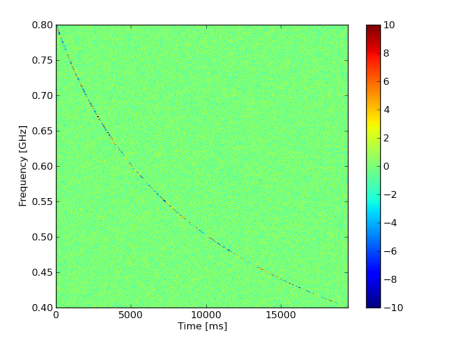
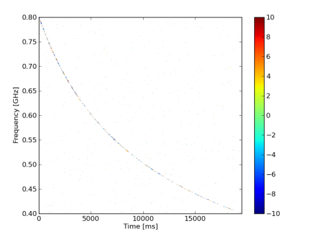
Figure 1: Top: simulated data; Bottom: truncated data (with $\tau=3.0$) which masks out most of the noises.

3 Application Test

In this section we test how our algorithm works with data. We first test it with simulation data (3.1), then test with real pulsar and FRB data (3.2).

3.1 Simulation Data

We generate a mock sample of observing data as a superposition of Gaussian noise and a dispersed FRB signal. The noise is independent and identically distributed (iid) Gaussian with a distribution $N(0,\sigma_{n}^{2})$, and the signal is also iid Gaussian with distribution $N(\mu,\sigma_{s}^{2})$. The parameters for the simulated data are set as $\sigma_{n}=1.0$, $\mu=3.0$, $\sigma_{s}=3.0$, and $\text{DM}=1000\,\text{pc cm}^{-3}$. The observing frequency range is 400 – 800 MHz, with 2048 frequency bins. The simulated data $I(t,f)$ is shown in the top panel of Figure 1. The simulated data is truncated with a threshold $\tau=3.0$. The truncated data $I_{m}$ is very sparse, as shown in the bottom panel of Figure 1, but the signal are mostly preserved.

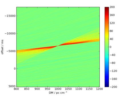
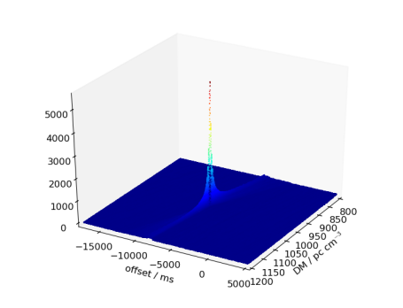
Figure 2: The Hough transform of the data shown in 2d (top) and 3d (bottom) plot.

The Hough transform of the truncated data is show in the range of ${\rm DM}\in[800,1200]\,\text{pc cm}^{-3}$ in Figure 2, from which we see the peak is just at the right location $\text{DM}=1000\,\text{pc cm}^{-3}$. Here we show both a 2D colour plot and a 3D plot for better illustration, as the strongest point in the figure is too narrow that it is hard to see in the 2D plot.

To understand the pulse detection sensitivity in the Hough transform, we consider the distribution in the Hough transform accumulator $A$. Here we first consider an ideal case, where the passband is flat, and the noise is uncorrelated white noise with Gaussian distribution. Here for definiteness, we consider a case where $N_{t}=N_{f}=512$, and $\sigma_{n}=1$, without any pulse signal. The distribution of $A$ for this pure noise case can be simulated easily with a random number generator. A typical data frame and its Hough transform with no truncation is shown in Fig.3. Each point in the time-frequency data frame is mapped to a line in the Hough transform, so we see many line features in the bottom panel of Fig.3.

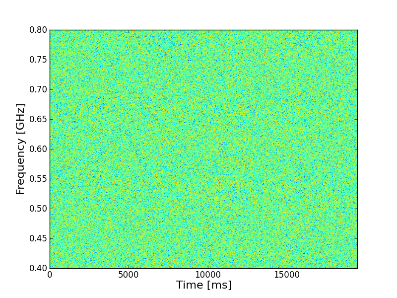
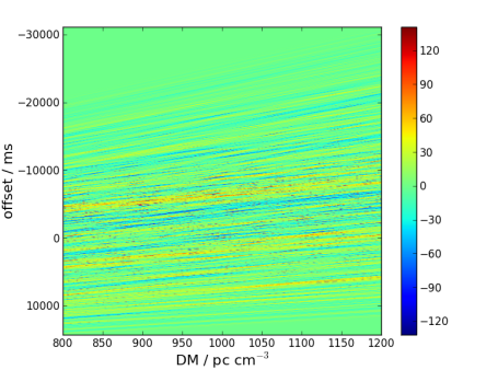
Figure 3: Top: A simulated noise data frame with $N_{t}=N_{f}=512$. Bottom: The Hough transform with no truncation.

We then compute the distribution function of $A$, and show the results in Fig. 4. From top to bottom the panels are $\tau=0$ (no truncation), $\tau=1$ (low truncation threshold), and $\tau=3$ (high truncation threshold) respectively. For the no truncation case ($\tau=0$) or low threshold case ( $\tau=1$), the distribution can be well fitted by a Laplace distribution:

$$f_{L}(A|\mu,b)=\frac{1}{2b}\exp\left(-\frac{|A-\mu|}{b}\right).$$ (12)

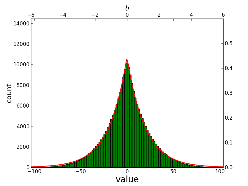
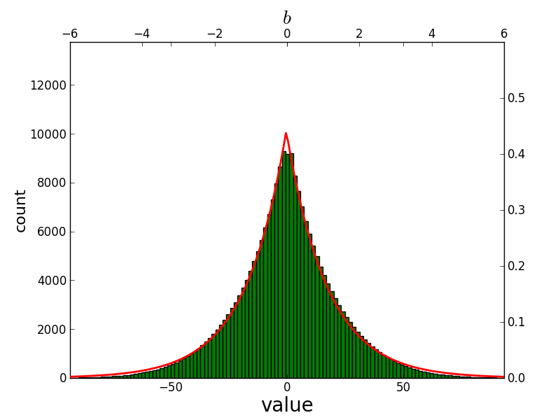
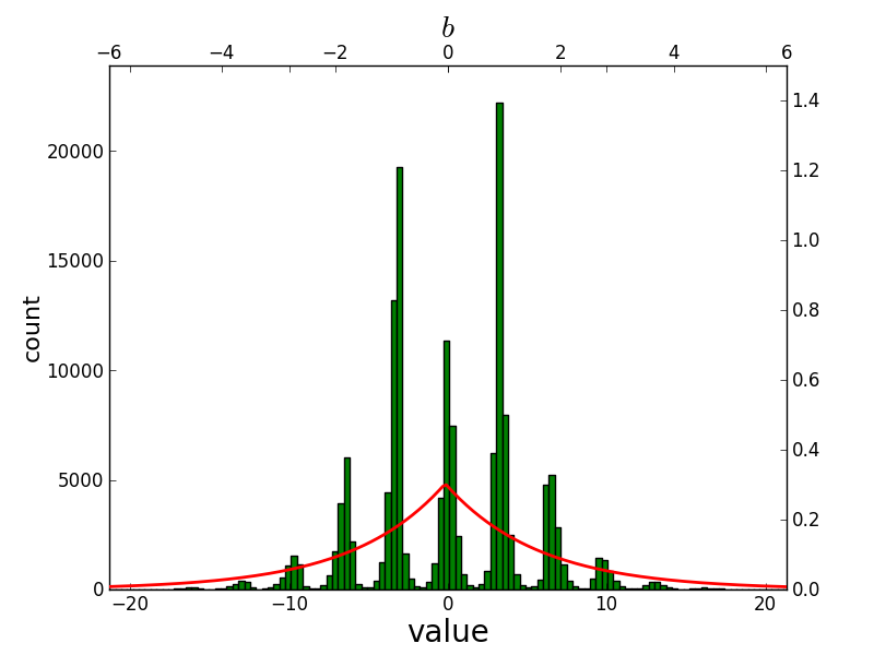
Figure 4: The Hough transform for a random noise image with threshold $\tau=0$ (top) and $\tau=1$ (middle) and $\tau=3$(bottom).

The distribution in the $\tau=3$ case exhibits an interesting behavior: evenly spaced peaks appear in the plot. These peaks originates from the discrete nature of the data: with high truncation threshold, only the relatively rare large fluctuation points remain in the time-frequency data frame. Each such point is transformed to a line in the Hough transform space, and contributes to a particular value of the elements of $A$ that the lines pass. According to Eq. (6), this contribution is also proportional to the value $I(t,f)$, which is a real number, i.e. has a continuous distribution, so naively one might think that any discreteness would be washed out and the distribution should be smooth. However, because the Gaussian distribution function of the noise is quite steep, when a particular high threshold is chosen, most survival points would be just above the threshold and have similar values. For example, for the truncation threshold $\tau=3$, most of the survival points would have a value $I_{p}$ just above $3$, they all map to lines with this intensity in $A$, and produce the first non-zero peak in the distribution of $A$. The crossing of these lines contributes a multiples of $I_{p}$ to the accumulator, so in the end we see these evenly spaced peaks in the $A$ distribution.

Based on the $A$ distribution function, one can choose a detection threshold for $A$, such that a false detection rate is below a preset value. For example, if we take the threshold to be $|A-\mu|>4b$, where $b$ is the parameter in the best-fit Laplace distribution, the false detection rate falls below 1.8%, or 0.9% if we only consider the positive end.

However, in the real application the situation would be much more complicated, as the passband may not be flat, the noise could be correlated, and there are also radio sources and RFIs. One will have to study the specific instrument and derive the noise generated $A$ distribution from the data.

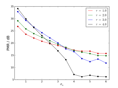
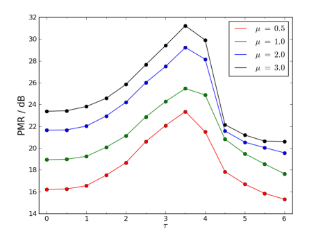
Figure 5: Top: the Peak-to-Median Ratio (PMR) shown in dB for different noise level $\sigma_{n}$, Bottom: the PMR (shown in dB) for different threshold $\tau$.

The Peak-to-Median Ratio $\text{PMR}=\max(A)/\text{median}(A_{>0})$ can be used as a measure of the relative strength of the highest peak to the noise background level, where $A_{>0}$ is the set of points for which the accumulator $A$ have positive values. The PMR as a function of the noise level $\sigma_{n}$ (with $\tau=1,2,3,4$) are plotted in the top panel of Figure 5 (shown in dB scale, i.e. $10\log_{10}{\rm PMR}$). We see that generally the PMR decreases monotonically as the noise level $\sigma_{n}$ increases, but up to $\sigma_{n}=6.0$ the overall PMR is still sufficiently high (PMR=14.3, or 11.5 dB) for detection. We also plot curves for different threshold value $\tau$. A higher threshold $\tau$ generally yields better SNR at low noise level $\sigma_{n}$, but at high noise level $\sigma_{n}$ this is reversed.

In the Bottom panel of Figure 5 we plot the PMR (shown in dB scale) as a function of the selected threshold $\tau$, for fixed noise level but different mean values. Initially the PMR value increases as $\tau$ increases, but then it decreases after reaching a peak. The truncation process does not only reduces computation complexity, but also throws away the relatively noisy data, while preserving the data where the signal is stronger, so the PMR is enhanced for some appropriate $\tau$, and a highest PMR is achieved at $\tau\sim 3.5$. The effect of truncation threshold may also depend on the mean background level. Several different mean value $\mu$ are plotted. However, as the curves show, although the peak value of PMR depends strongly on the $\mu$ value, for low $\mu$ the peak PMR is small (e.g. when $\mu=0.5$, we can get a peak PMR of 117.9(20.7 dB), while for $\mu=3$ the peak PMR is up to $\sim 1350$(31.3 dB). However, the value that achives highest PMR does not change much. Even in the case when $\mu=0$, as long as $\sigma_{s}$ is much higher than $\sigma_{n}$, the pulse can be detected by the Hough transform method, for example, when $\mu=0$, $\sigma_{s}=3.0$, while $\sigma_{n}=1.0$, we obtain a PMR of 19.6 (12.9 dB) when using a truncation threshold $\tau=3.0$.

These results show that the Hough transform pulse detection method works quite well for relatively strong S/N pulse signals. However, the selection of the truncation threshold is a delicate problem, a lower threshold is needed to detect the low signal-to-noise ratio pulses, but the computation time increases drastically at lower threshold. There is a trade-off between the computation savings and the mis-detection rate, one needs to select the threshold according to practical needs.

Event	Telescope	DM [pc cm-3]	Speak,obs [Jy]	Fobs [Jy ms]	Ref
FRB 010125	Parkes	790(3)	0.30	2.82	Burke-Spolaor & Bannister (2014)
FRB 010621	Parkes	745(10)	0.41	2.87	Keane et al. (2011)
FRB 010724	Parkes	375	$>$$30.00^{+10.00}_{-10.00}$	$>$$150.00$	Lorimer et al. (2007)
FRB 110220	Parkes	944.38(5)	$1.30^{+0.00}_{-0.00}$	$7.28^{+0.13}_{0.13}$	Thornton et al. (2013)
FRB 110523	GBT	623.30(6)	0.60	1.04	Masui et al. (2015)
FRB 110626	Parkes	723.0(3)	0.40	0.56	Thornton et al. (2013)
FRB 110703	Parkes	1103.6(7)	0.50	2.15	Thornton et al. (2013)
FRB 120127	Parkes	553.3(3)	0.50	0.55	Thornton et al. (2013)
FRB 140514	Parkes	562.7(6)	$0.47^{+0.11}_{-0.08}$	$1.32^{+2.34}_{-0.50}$	Petroff et al. (2015a)

Table 1: FRBs used in this paper and some of their parameters.

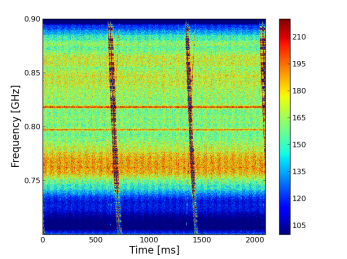
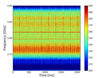
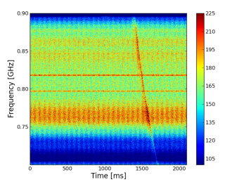
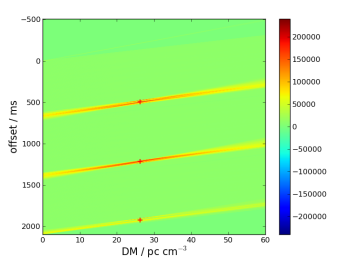
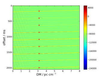
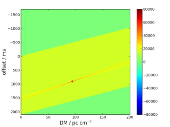
Figure 6: The observing data (top) and the corresponding Hough transform (bottom) of pulsars B0329+54, B1929+10, and B2319+60 respectively. The detected peaks are marked by a red $+$ in the transformed image.

3.2 Real Pulsar and FRB Data

We first apply our method to real observation data of three pulsars, i.e. B0329+54, B1929+10, and B2319+60 taken by the Green Bank Telescope (GBT). We chose a truncation threshold $\tau=3.0$, and used a $4000\times 2000$ accumulator $A(t_{0},d)$ with a DM range $[0,100]\,\text{pc cm}^{-3}$. The Hough transform for an example of the data lasting about 2 seconds containing several pulses are shown in the top panels of Figure 6 for the three pulsars. The corresponding Hough transform are plotted in the bottom panels. and we have also marked the detected peaks by a red $+$ in the transformed images.

In the data shown in the plot, there is one single pulse track for B2319+60 (right column) with DM $=94.591\text{pc cm}^{-3}$, while for B0329+54 (left column) there are three tracks with DM $=26.7641\text{pc cm}^{-3}$, and many tracks for B1929+10 (middle row) with DM $=3.18321\text{pc cm}^{-3}$. Each pulse track in the observed data has been transformed to a bundle of lines crossing at the same point, which can be detected easily with the program (though when plotted in Figure 6 they are visually not so obvious due to the small size of the peak point, to aid the eye we marked these by a cross in the figure.) If there are more than one cross points corresponding to more than one pulse track in the observed data, they all have the same DM value, which are all very close to the values measured with other programs (e.g. those given by psrcat in Manchester et al. (2005)). Note there are two strong narrow frequency band RFIs in the middle of each data, but they do not show in the corresponding Hough transformed images, as the Hough transform automatically rejects them.

We also apply our method to several FRB event data, including eight FRBs observed by the Parkes telescope taken from the FRB Catalogue compiled by Petroff et al. (2016), and one FRB event data (FRB 110523) observed by the GBT (Masui et al., 2015). These FRBs are listed in Table 1. Observing data of these FRBs are shown in Fig.7, and their corresponding Hough transformed result are shown in Fig.8, with the detected peaks marked by red $+$ signs in the transformed image.

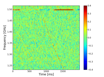
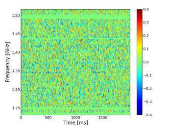
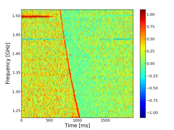
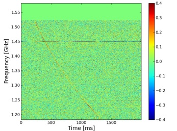
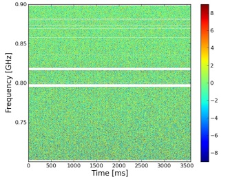
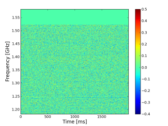
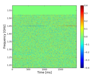
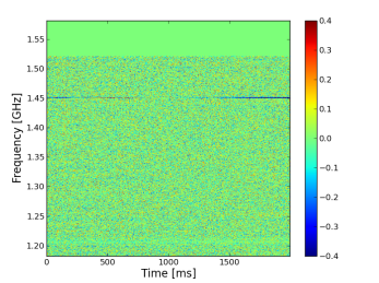
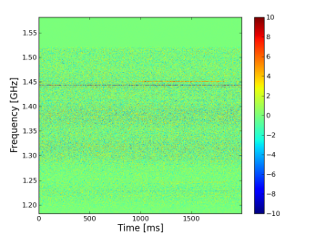
Figure 7: The observation data for FRB 010125, FRB 010621, FRB 010724(top row, left to right), FRB 110220, FRB 110523, FRB 110626 (middle row, left to right), and FRB 110703, FRB 120127, FRB 140514(bottom row, left to right).

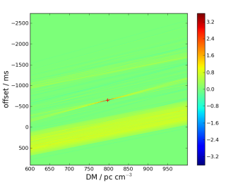
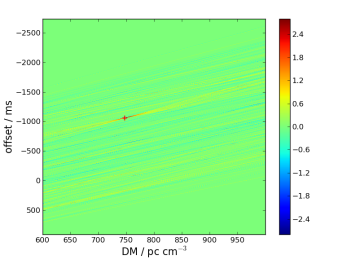
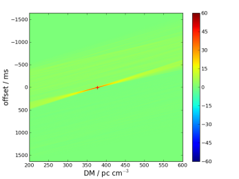
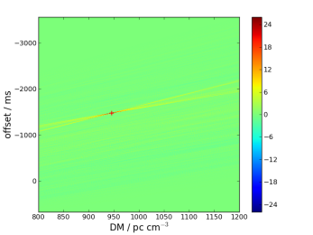
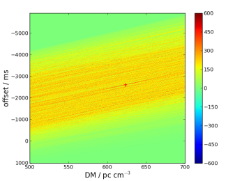
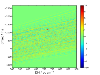
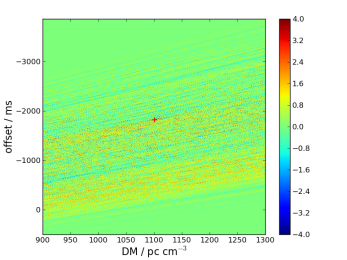
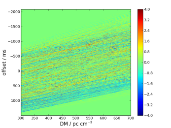
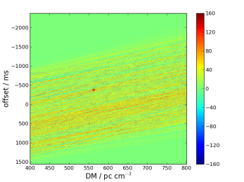
Figure 8: The Hough transform matrix $A$ for the 9 FRBs shown in the figure above, in the same order. The detected peaks are marked by a red $+$ in the transformed image.

We tried a few different truncation thresholds, then apply the Hough transform to search for them. We found that in most cases a threshold $\tau=3.0$ is sufficient, but for a few weaker ones lower thresholds are required, specifically, $\tau=2.5$ for FRB 120127, $\tau=2.0$ for FRB 010724, and $\tau=1.0$ for FRB 110626. We see from Table 1 that FRB 120127 and FRB 110626 have very low peak intensity S_peak,obs and integrated intensity F_obs relative to other ones, lower thresholds are needed for their detection. The lower threshold would require larger amount of computation, while in higher threshold they might be missed. The case of FRB 010724 is somewhat different, its pulse signal is fairly strong, but it could also only be detected with a lower threshold, say $\tau=2.0$. This may be related to its non-uniform background noise, as can be seen clearly in Figure 7, the background noise has big difference between the left and right part of the pulse track, this affects the background mean subtraction, and further makes the pulse detection harder. Nevertheless, all FRBs can be successfully detected by using the Hough transform method, and the DM values obtained from the detected peaks are very close to the public values as listed in Table 1.

Note that in our processing, we have not make any special treatment for the RFIs or any other outliers before the Hough transform. For all data except for the FRB 110523, we have used the raw data, the only processing besides the truncation and Hough transform described above is rebinning in time direction to reduce the amount of data. For FRB 110523 the pre-processed data is available to us, which has been calibrated and RFI flagged. We can see from the data images, many of the data has RFIs or outliers in them, usually single frequency or narrow band RFIs, some are much stronger than the pulse signals. As we discussed in Section. 2.3, they should not have much impact on the detection based on the Hough transform, and this is confirmed by the results.

In the present treatment, the search for the peak in $A$ is conducted at the single pixel level, i.e. we search the pixel which has the maximum value. This may not achieve the highest sensitivity, for the true peak may be located somewhere between the accumulator pixels, so that each of its neighbouring pixels has a relatively high value, but not as high as it would have been if the peak is right centered on that pixel.

A related issue is, in the above we have assumed that the time width of the pulse signal is within one sample, however, the burst may last more than one sample width, i.e. the signal track is not a curve but a band of finite width. In such cases, the Hough transform will map the band into several neighbouring pixels in the accumulator space, i.e. $A(d,t_{0})$ of the same $d$ but successive $t_{0}$. For optimal detection sensitivity, the width of the signal should be nearly equal to the sample time width. A practical implementation of pulse search program needs to deal with this issue. In some search programs, this can be achieved by rebinning the data along the time direction, up to a physically plausible maximum width, and make trial search with the larger sample time widths. In the Hough transform, this process can be achieved simply by integrating the neighbouring pixels with kernels of different widths. Here the Hough transform may also have some advantages over other methods, for instead of blindly rebinning along time direction for all data points, here we may pick a small number of peaks in the accumulator space, and try integrating with kernels of different widths, in practice make weighted average with different weights. The amount of computation in this part is again much reduced compared with rebinning all points. This is also more flexible than rebinning, and can even be made adaptively. We shall leave the detailed investigation of these issues to future studies.

4 Discussions

We have presented a simple and fast radio bursts detection and incoherence dedispersion method based on Hough transform. The $f^{-2}$ burst curve in the observed time stream data is mapped to be a bundle of straight line in the transformed space which crossed the same point determined by the dispersion measure of the burst. By detecting the peak, we can detect the bursts and measure their dispersion measures. The advantage of the method is that by setting an appropriate truncation threshold, it has a low computational complexity of $O(\text{max}(N_{t},N_{f})N_{d})$, which is much lower than the existing algorithms. Wise choice of noise truncation threshold may also improve the detection sensitivity. The method automatically rejects most commonly encountered RFIs, making it good for online (real time) bursts detection. We have shown its effectiveness by simulation and application to the real pulsar and FRB observing data.

The truncation of data which saves much computation is particularly important for real-time detection. The computation time for several different truncation thresholds are shown in Figure 9 for FRB 010125 with data dimension of $96\times 500$ and for FRB 110220 with data dimension of $1024\times 500$). The computation time are measured on an Intel Xeon E5-2670 2.60 GHz CPU using program written in the C programming language. For comparison, the brute force dedispersion is also implemented in the same computing environment, the algorithms run with a single thread for the same range and resolution of dispersion measure, and the time reported is the average time for 10 runs. Note that here we have included the background subtraction time in the reported computation time of the Hough transform method, where for the computation of the median (and also the MAD), we have simply implemented it by first sorting the array, which is not a very fast method for median computation, more effective methods exists, for example, the median of medians algorithm (Blum et al., 1973), which finds an approximate median in linear time. If some of the faster median computing methods are used, the performance of the Hough transform method can be further improved. But even for this simple implementation, the computation time of the Hough transform method with a truncation threshold $\tau\geq 1.0$ is less than that of the brute force method, and the computation times decays exponentially with the increasing truncate threshold $\tau$. The exponential fall off is what we expected for the survival number of pixels by thresholding a Gaussian background. We also plot the survival function $2\Phi(-\tau)=2[1-\Phi(\tau)]$ of the normal distribution in Figure 9 for comparison.

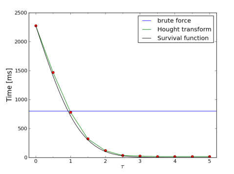
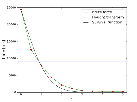
Figure 9: Comparison of the computation time for the Hough transform method with different truncation threshold $\tau$ and the brute force method. Top panel for FRB 010125, Bottom panel for FRB 110220. The black curve gives the scaled survival function $2\Phi(-\tau)=2[1-\Phi(\tau)]$ of the normal distribution, which overlaps the computation time curve at the value of $\tau=0$.

The Hough transform method is readily applicable to online (nearly real time) processing. It can also be easily parallelized to speed up the computation, by either partitioning the points in the truncated image to $N$ parts and do the Hough transform for these points in each part independently, with the total accumulator given by the sum, or by partitioning the computation of different dispersion measures. The Hough transform algorithm itself can also be parallelized (Ben-Tzvi & Sandler, 1989; Lu et al., 2013), or be accelerated with graphic processing units (GPUs) (Tomagou et al., 2013; Patil et al., 2016). GPUs are now widely used in computing-intensive environment. With very large number of computing cores, a GPU can achieve orders of magnitude higher computing speed than a CPU for an appropriate problem, by dividing the work load among thousands of threads which run in parallel. Indeed, given the much higher raw computing speed, even the brute force de-dispersion could be handled with the GPUs in short time. Nevertheless, improving the computing efficiency is still important, for the data rate is also rapidly increasing. For example, thousands of beams can be formed by a large interferometer array such as the SKA, each with very large bandwidth, and searching the FRB for these many beams remain a computationally challenging task.

We now consider the Hough transform with GPU. We first perform the truncation on a CPU, as handling conditional statements is not a strong point for GPU. The truncated array is then send to the GPU for Hough transform. The GPU can perform this computation by distributing it over the large number of cores available. Suppose after truncation the number of remaining pixels is $N$, with $N\leq N_{t}N_{f}$, and number of DM trial value $N_{d}$, we may launch for example a total of $NN_{d}$ threads, each compute the accumulator values for this pixel. In this case the GPU computing cores and the threads need to share the common memory of the total accumulator array, which is a sum of the accumulator array of all threads, but otherwise the computation of the threads are independent.

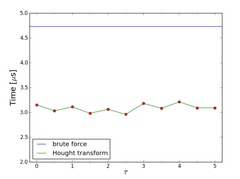
Figure 10: The computation time with GPU as a function of truncation threshold $\tau$.

In Fig. 10 we show the computation time using a GPU server. The GPU we used is an NVIDIA GTX 1080TI. For the test the data frame has a size of $N_{f}=1024,N_{t}=512,N_{d}=2000$. We plot both the time needed for the brute force method and the Hough transform method. As can be seen from the figure, compared with the CPU, the GPU computation takes very short time. The Hough transform takes slightly more than half of the time of the brute force computation, and unlike the CPU case, it is almost independent of the truncation threshold. This is because in the case of GPU, although $N$ is larger for lower threshold $\tau$, for this parameter range the GPU can launch a total number of $NN_{d}$ threads. The time needed for computation is essentially the time needed for one thread to complete its computation, plus the time for each process to communicate its result, which is a very small amount in the present case. Thus, with GPU one can achieve high sensitivity by choosing a low truncation threshold. However, as point out above, for large arrays many beams may be formed and feed to the GPU for computation. We should also note that In a practical implementation, there will also be many restrictions which reduce the computing speed, for example the data transfer rate may severely limit the amount of the data that a GPU can handle, so the computation speed is much slower than indicated by Fig.10. Reducing the computational complexity is still quite meaningful at present.

In this paper we have focused primarily on the concept and theoretical aspects of the Hough transform method for radio burst detection. We demonstrated the application of this method by simulation and some real pulsar and FRB data, though for real application there are still some practical issues to be addressed, for example, determining the implementation and optimisation of the Hough transform algorithm, the parallelism and acceleration strategy; selecting the appropriate truncation threshold as a trade-off between the sensitivity and the computation time; developing peak searching algorithm which can integrate the neighbouring pixels with different kernel size, etc. These are beyond the scope of this paper, we leave them for future studies.

References

- Ben-Tzvi & Sandler (1989) Ben-Tzvi D., Sandler M., 1989, Microprocessing and Microprogramming, 27, 147
- Blum et al. (1973) Blum M., Floyd R. W., Pratt V., Rivest R. L., Tarjan R. E., 1973, Journal of Computer and System Sciences, 7, 448
- Burke-Spolaor & Bannister (2014) Burke-Spolaor S., Bannister K. W., 2014, ApJ, 792, 19
- CHIME Scientific Collaboration et al. (2017) CHIME Scientific Collaboration et al., 2017, preprint, (arXiv:1702.08040)
- Fridman (2008) Fridman P. A., 2008, AJ, 135, 1810
- Fridman (2010) Fridman P. A., 2010, MNRAS, 409, 808
- Hampel (1974) Hampel F. R., 1974, Journal of the American Statistical Association, 69, 383
- Hough (1962) Hough P., 1962, METHOD AND MEANS FOR RECOGNIZING COMPLEX PATTERNS, US Patent 3,069,654
- Keane et al. (2011) Keane E. F., Kramer M., Lyne A. G., Stappers B. W., McLaughlin M. A., 2011, MNRAS, 415, 3065
- Leys et al. (2013) Leys C., Ley C., Klein O., Bernard P., Licata L., 2013, Journal of Experimental Social Psychology, 49, 764
- Lorimer et al. (2007) Lorimer D. R., Bailes M., McLaughlin M. A., Narkevic D. J., Crawford F., 2007, Science, 318, 777
- Lu et al. (2013) Lu X., Song L., Shen S., He K., Yu S., Ling N., 2013, Sensors (Basel, Switzerland), 13, 9223
- Manchester et al. (2005) Manchester R. N., Hobbs G. B., Teoh A., Hobbs M., 2005, AJ, 129, 1993
- Masui et al. (2015) Masui K., et al., 2015, Nature, 528, 523
- Patil et al. (2016) Patil P. R., Patil M. D., Vyawahare V. A., 2016, in 2016 International Conference on Communication and Signal Processing (ICCSP). pp 1584–1588, doi:10.1109/ICCSP.2016.7754427
- Petroff et al. (2015a) Petroff E., et al., 2015a, MNRAS, 447, 246
- Petroff et al. (2015b) Petroff E., et al., 2015b, MNRAS, 451, 3933
- Petroff et al. (2016) Petroff E., et al., 2016, Publ. Astron. Soc. Australia, 33, e045
- Radon (1917) Radon J., 1917, Berichte Sächsische Akademie der Wissenschaften, Leipzig, Math.-Phys. Kl., 69, 262
- Rousseeuw & Croux (1993) Rousseeuw P. J., Croux C., 1993, Journal of the American Statistical Association, 88
- Taylor (1974) Taylor J. H., 1974, A&AS, 15, 367
- Thornton et al. (2013) Thornton D., et al., 2013, Science, 341, 53
- Tomagou et al. (2013) Tomagou N., Nakano K., Ito Y., 2013, Bulletin of Networking, Computing, Systems, and Software, 2
- Zackay & Ofek (2014) Zackay B., Ofek E. O., 2014, preprint, (arXiv:1411.5373)
- van Ginkel et al. (2004) van Ginkel M., Hendriks C. L., van Vliet L., 2004, A short introduction to the Radon and Hough transforms and how they relate to each other