Exact isovector pairing in a shell-model framework:
Role of proton-neutron correlations in isobaric analog states

Abstract

We utilize a nuclear shell model Hamiltonian with only two adjustable parameters to generate, for the first time, exact solutions for pairing correlations for light to medium-mass nuclei, including the challenging proton-neutron pairs, while also identifying the primary physics involved. In addition to single-particle energy and Coulomb potential terms, the shell model Hamiltonian consists of an isovector $T=1$ pairing interaction and an average proton-neutron isoscalar $T=0$ interaction, where the $T=0$ term describes the average interaction between non-paired protons and neutrons. This Hamiltonian is exactly solvable, where, utilizing 3 to 7 single-particle energy levels, we reproduce experimental data for 0⁺ state energies for isotopes with mass $A=10$ through $A=62$ exceptionally well including isotopes from He to Ge. Additionally, we isolate effects due to like-particle and proton-neutron pairing, provide estimates for the total and proton-neutron pairing gaps, and reproduce $N$ (neutron) = $Z$ (proton) irregularity. These results provide a further understanding for the key role of proton-neutron pairing correlations in nuclei, which is especially important for waiting-point nuclei on the rp-path of nucleosynthesis.

I Introduction

Since a pairing model was first applied to nuclei by Bohr, Mottelson, and Pines Bohr et al. (1958), studies have repeatedly found pairing correlations to have a profound influence on nuclear structure Belyaev (1958). A better understanding of pairing features in nuclei could greatly benefit other areas of research, such as superfluidity in neutron stars Bennemann and Ketterson (2013); Gezerlis et al. (2014), pairing correlations in nuclear matter Drischler et al. (2017); Ding et al. (2016); Burrello et al. (2016) and nuclei around closed shells Bohr and Mottelson (1975). While pairing correlations among like-particles, e.g., proton-proton ($pp$) and neutron-neutron ($nn$) pairing, have been described through numerous methods Helmers (1961); Flowers and Szpikowski (1964); Lane and Hayward (1964); Hecht (1965a); Henderson et al. (2014) and are well understood, proton-neutron ($pn$) pairing has been less studied due to its complexity Hecht (1965b); Van Isacker (2013); Pan and Draayer (2002); Sviratcheva et al. (2004a); Engel et al. (1997); PAN201886; PAN20181. For example, current approaches for pairing in the continuum have been addressed Mercenne et al. (2017); Betan (2017, 2012) but solely for like-particle pairing. An accurate treatment of the challenging $pn$ pairing interaction has been suggested to be important for understanding waiting-point nuclei in rapid-proton capture nucleosynthesis Sharma and Sharma (2010, 2009); Pruet and Fuller (2003) and may play a role in neutrinoless double-beta decay ($0\nu\beta\beta$) Hinohara and Engel (2014); Jiao et al. (2017). Therefore, exact analytic solutions for both like-particle and $pn$ pairing are of great interest.

Albeit restricted to degenerate single-particle energies, exact solutions to like-particle and $pn$ pairing interactions can be achieved through the $T=1$ charge-independent pairing Hamiltonian constructed using generators of the quasispin group Sp_j(4), where $j$ indicates the orbits utilized in the model space and $T$ corresponds to the isospin Hecht (1965b); Launey (2003). For non-degenerate single-particle energies, approximate numerical solutions can be attained through the BCS formalism Šimkovic et al. (2003); Sandulescu et al. (2009); Baranger (1961); Brémond and Valatin (1963); Flowers and Vujičić (1963). Some studies utilize the algebraic Bethe ansatz method with an infinite-dimensional Lie algebra Dukelsky et al. (2002); Pan et al. (1998); Pan and Draayer (1998, 1999); Pan et al. (2000); Richardson (1966a); Chen and Richardson (1971); Hsi-Tseng and Richardson (1973) and other methods Richardson (1965, 1966b); Richardson and Sherman (1964a, b); Dukelsky et al. (2011); Qi and Chen (2015); Dukelsky (2014) provide exact solutions for systems with like-particle pairing or for systems with two or fewer pairs.

In this paper, we present a new shell model Hamiltonian that yields exact analytic solutions for the lowest isovector-paired $0^{+}$ states for up to six nucleons (three pairs). The Hamiltonian, adapted from Ref. Sviratcheva et al. (2004a) where degenerate energies have been considered, consists of a single-particle energy term, Coulomb potential term, and includes an isovector $T=1$ pairing interaction and an isoscalar $T=0$ proton-neutron interaction that accounts for the average interaction between non-paired nucleons. The model utilizes the analytic solutions to isovector pairs in non-degenerate single-particle levels that are derived in Ref. Pan and Draayer (2002) for up to three pairs. However, when considering three or more pairs highly nonlinear equations appear and require sophisticated solution mechanisms Guan et al. (2012). Here, we report applications of such solutions to light through medium-mass nuclei including the challenging $pn$ pairs. We also identify the primary physics involved through an analysis of the staggering behavior of our results and pairing gap estimates.

II Theoretical Formalism

Algebraic solutions to a $T=1$ charge-independent pairing Hamiltonian that utilizes single-particle energies of the $j$th orbit, $\epsilon_{j}$, which can be derived from the spherical shell model, are introduced in Ref. Pan and Draayer (2002). These solutions are for $J^{\pi}=0^{+}$ states of $2k$ nucleons and include both like-particle and $pn$ pairs, where $k$ is the total number of pairs. To describe ground states and $0^{+}$ isobaric analog states in nuclei it is important to consider the Coulomb potential and an isoscalar $T=0$ $pn$ interaction Sviratcheva et al. (2004a) in addition to the isovector pairing. In particular, our model Hamiltonian is expressed as

$$\hat{H}=\sum_{j}\varepsilon_{j}N_{j} - G\sum_{jj^{{}^{\prime}}\mu}A^{\dagger}_{j,\mu}A_{j^{{}^{\prime}},\mu}$$

$$+ \alpha\Bigg{(}\hat{T}^{2}-\frac{N}{2}\bigg{(}\frac{N}{2}+1\bigg{)}\Bigg{)}+V_{\text{Coul}},$$

where $G>0$ is the pairing strength, and $\alpha$ is the strength of the additional isoscalar $T=0$ interaction, which can be understood as the average interaction between nonpaired protons and neutrons in a $T=1$ pair as shown in Ref. Launey (2003) (also related to the symmetry term). The nucleon number operator $N_{j}$, pair creation $A^{\dagger}_{j,\mu}$ and annihilation $A_{j,\mu}=(A^{\dagger}_{j,\mu})^{\dagger}$ operators, where $\mu=+,-,0$ indicates $pp$, $nn$, and $pn$ pairs, respectively, together with the isospin operators $\hat{T}_{j,\pm 1}$ and $\hat{T}_{j,0}$ are generators of the Sp_j(4) group. The total number operator is given by $N=\sum_{j}N_{j}$, which is also $N=2k$, and $V_{\text{Coul}}$ denotes the Coulomb interaction. The Hamiltonian is initially solved for the first two terms in Eq. (II), as described in the next section, resulting in eigenstates that have $k$, $T$, and $T_{z}$ as good quantum numbers (or, equivalently, proton and neutron numbers along with $T$); in this basis the $\alpha$ term is diagonal, resulting in additional energy given by $\alpha(T(T+1)-k(k+1))$. The Coulomb term is also diagonal and its contribution is accounted by an estimate given in Ref. Retamosa et al. (1997), as described in Sec. II.2.

II.1 Exact isovector pairing solutions for up to six nucleons

Exact solutions for non-degenerate single-particle energies and isovector $T=1$ pairing interaction [first two terms of Eq. (II)] for $k\leq 3$ are derived for selected permutations of the permutation group $S_{k}$ in Ref. Pan and Draayer (2002). As described in Ref. Pan and Draayer (2002), the method uses elements of the Gaudin algebra $\mathcal{G}$(Sp(4)), $A^{\dagger}_{\mu}(x)=\sum_{j}\frac{A^{\dagger}_{j,\mu}}{1+\varepsilon_{j}x}$, $A_{\mu}(x)=\sum_{j}\frac{A_{j,\mu}}{1+\varepsilon_{j}x}$, $T_{\mu}(x)=\sum_{j}\frac{T_{j,\mu}}{1+\varepsilon_{j}x}$, and $N(x)=\sum_{j}\frac{N_{j,\mu}}{1+\varepsilon_{j}x}$, where $x=\{x_{1},x_{2},\dots,x_{k}\}$ are spectral parameters for $k$ pairs. Hence, one can solve the Hamiltonian, $\hat{H}=\left.\partial N/\partial x\right|_{x=0}+GA^{\dagger}(0)\cdot A(0)$ using the Bethe ansatz wave function $\left|k;\zeta;[\lambda]_{k},TT_{z}\right\rangle=\sum_{P\in S_{k}}Q^{[\lambda]}(x_{P_{1}},x_{P_{2}},\dots,x_{P_{k}})$ $\left\{A^{\dagger}(x_{P_{1}})\times A^{\dagger}(x_{P_{k}})\times\dots\times A^{\dagger}(x_{P_{k}})\right\}^{TT_{z}}\left|0\right\rangle$, that describes a $k$-paired state with $\left|0\right\rangle$ the seniority-zero state, where $[\lambda]_{k}$ is an irrep of the permutation group $S_{k}$ containing $k$ boxes in the corresponding Young diagram and $P$ labels all possible permutations. As a result, the expansion coefficients $Q^{[\lambda]}$ and the spectral parameters, $x_{1},\dots,x_{k}$, are determined. In Ref. Pan and Draayer (2002) solutions are derived for the cases $k=1$, $T=1$ along with $k=2$ and $3$ for $T=0,\dots,k$.

It is important to note that this method leads to highly nonlinear equations that become more challenging to solve as $k$ increases. Therefore, to find solutions and reduce the number of singularities we have modified the spectral parameters of Ref. Pan and Draayer (2002), such that in numerical calculations we use $y_{i}\equiv 2/x_{i}$ where $i=1,2,\dots,k$. Additionally, we utilize an average single-particle energy $\epsilon_{\text{avg}}$ defined as

$$\epsilon_{avg}=\frac{\sum\limits_{j}(\Omega_{j}\epsilon_{j})}{\sum\limits_{j}\Omega_{j}},$$ (2)

where $\Omega_{j}=j+\frac{1}{2}$ is the $j$-level degeneracy. Hence, the energies utilized are taken with respect to this average energy, $\varepsilon_{j}=\epsilon_{j}-\epsilon_{avg}$. In the appendix we briefly outline the main equations, which have been derived in Ref. Pan and Draayer (2002), in terms of the different variables used in the present numerical calculations.

II.2 Coulomb potential

We include the Coulomb potential ($V_{\text{Coul}}$) by using estimates provided in Ref. Retamosa et al. (1997). Defining $N_{+}$, $N_{-}$, and $A$ as the valence proton, neutron, and the atomic numbers of nuclei, respectively, we first calculate $V_{\text{Coul}}$ of isotopes with $N_{+}=N_{-}$. These energies are then used to calculate $V_{\text{Coul}}$ when $Z>Z_{s}$ and $Z<Z_{s}$. If $N_{+}=N_{-}$ and $N_{+}\leq 20$ then $V_{\text{Coul}}$ is given as

$$V_{\text{Coul}}(A,N_{-})=0.162N_{-}^{2}+0.95N_{-}-18.25.$$ (3)

However, if $N_{+}=N_{-}$ and $N_{+}>20$ then $V_{\text{Coul}}$ is defined as

$$V_{\text{Coul}}(A,N_{-})=0.125N_{-}^{2}+2.35N_{-}-31.53.$$ (4)

Next we calculate $V_{\text{Coul}}$ when $N_{+}\neq N_{-}$ and $N_{+}>N_{-}$, where the relation for this case is

$$V_{\text{Coul}}(A,N_{+}) = V_{\text{Coul}}(A,N_{+}-1)$$

$$+ 1.44\frac{N_{+}-\frac{1}{2}}{A^{1/3}}-1.02.$$

However, if $N_{+}\neq N_{-}$ and $N_{+}<N_{-}$ then $V_{\text{Coul}}$ is

$$V_{\text{Coul}}(A,N_{+}) = V_{\text{Coul}}(A,N_{+}+1)$$

$$- 1.44\frac{N_{+}+\frac{1}{2}}{A^{1/3}}+1.02.$$

The relations (3-II.2) were used to calculate the Coulomb potentials for even-$A$ isotopes in the mass ranges $A=10-16$, $A=34-46$, and $A=50-56$. These energies were accounted for when reproducing the experimental energy spectra for these mass ranges.

III Results and Discussion

The present model, which accounts for both $pn$ and like-particle pairing, has been successfully applied to even-$A$ nuclei for up to six particles above and below the ¹⁶O, ⁴⁰Ca, and ⁵⁶Ni cores. In particular, using only two adjustable parameters, $G$ and $\alpha$, and experimentally deduced single-particle energies we calculate exact solutions for the $J^{\pi}=0^{+}$ binding energies in even-even ($ee$) nuclei and the lowest isobaric analog $0^{+}$ excited states in odd-odd ($oo$) nuclei (which correspond to the ground state of the even-even neighbor), together with pair-excitation $0^{+}$ states. Using these solutions we are able to reproduce the experimental energy spectra as well as utilize discrete derivatives of the energy function to describe fine pairing features of these light to medium-mass nuclei off closed shells.

III.1 Energy spectra for isotopes around ${}^{\textbf{16}}$O, ${}^{\textbf{40}}$Ca, and ${}^{\textbf{56}}$Ni

In our model we use single-particle energies deduced from the experimental energy spectrum of $A_{\text{core}}\pm 1$ nuclei for a core of mass $A_{\text{core}}$. These single-particle energies are non-degenerate, thus providing more accurate solutions as compared to an earlier algebraic model based on the Sp(4) group Sviratcheva et al. (2004a), or equivalently on the O(5) group, that utilizes the same Hamiltonian. Indeed, it is crucial for our model to consider non-degenerate energies due to the comparatively large energy gap between levels, which is on the order of approximately 1 MeV. The experimentally deduced single-particle energies and the model parameters utilized in the Hamiltonian are listed in Table 1 for their respective cores. It should be noted that the $0d_{5/2}$ single-particle energy level in the ⁵⁵Ni energy spectrum has yet to be experimentally determined, leaving us unable to utilize this energy in our Hamiltonian. This truncation in the model space may account for deviations from experiment for even-$A$ isotopes in the mass range $50\leq A\leq 54$.

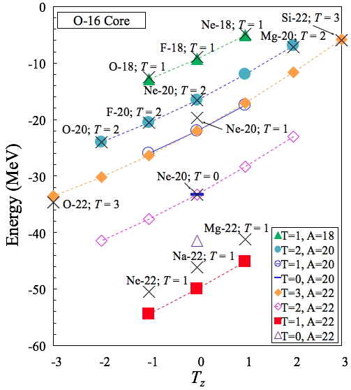
(a)

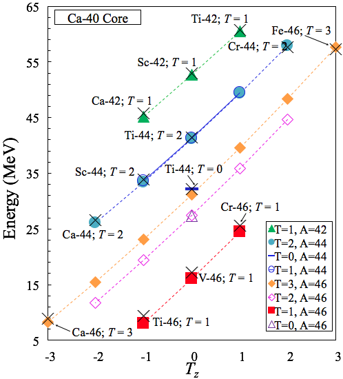
(b)

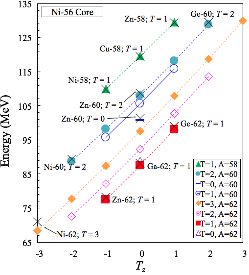
(c)

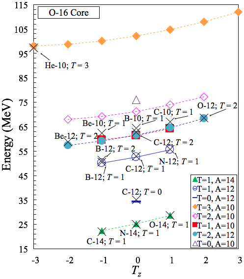
(d)

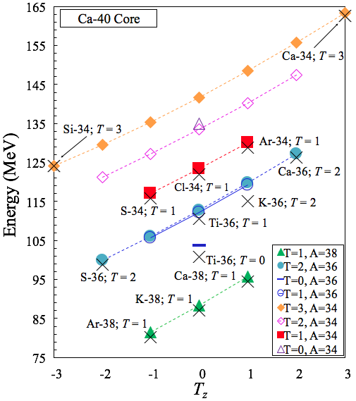
(e)

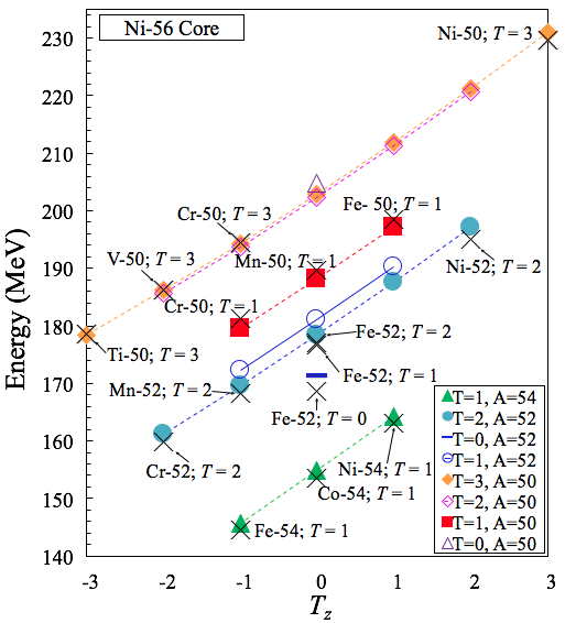
(f)

Figure 1: (Color online) Theoretical energy spectra (colored shapes) compared to experiment (black crosses) for $0^{+};0,..,3$ binding energies and lowest isobaric analog $0^{+};0,..,3$ excited states of isotopes above and below the (a) ¹⁶O core; (b) ⁴⁰Ca core; (c) ⁵⁶Ni core.

The model parameters were determined by first adjusting $G$ for the $k=T$ cases where the $\alpha$-term of the Hamiltonian has zero contribution to the $0^{+}$ energy of the isobaric analog states. Next, $\alpha$ was adjusted for the $k\neq T$ cases where both the $pn$ isoscalar and isovector interactions contribute significantly. We find that, while typically particles and holes (above and below a core, respectively) can be described by the same $G$ and $\alpha$ values, a larger pairing strength, $G$, is required for the lightest nuclei below the ¹⁶O core in the mass range 10 $\leq$ $A$ $\leq$ 14. This, however, is in agreement with $G$ proportional to $(17\pm 1)/A$ and $\alpha$ proportional to $36\pm 3/A$, which is supporded by earlier estimates Bohr and Mottelson (1975).

Our model very closely reproduces the energy of the lowest $0^{+},\ T=0,\dots,3$ states of $ee$ and $oo$ nuclei for up to six particles above and below the ¹⁶O, ⁴⁰Ca, and ⁵⁶Ni cores (Fig. 1(d)). The theoretical and experimental energy spectrum of individual isotopes are listed for allowed isospin values. Though only like-particle pairing occurs when $k=|T_{z}|$, our model accounts for $pn$ pairing as well, which is a significant feature, as it permits the calculation of the binding energies for isotopes when $k\neq|T_{z}|$ and the especially interesting $N=Z$ case.

Core	Particles (MeV)	Holes (MeV)
16O	$G=0.55$	$G=1.65$
	$\alpha=2.445$
	$\varepsilon_{0d_{5/2}}=-4.14$	$\varepsilon_{0p_{1/2}}=15.66$
	$\varepsilon_{1s_{1/2}}=-3.27$	$\varepsilon_{0p_{3/2}}=21.84$
	$\varepsilon_{0p_{3/2}}=0.94$	$\varepsilon_{0s_{1/2}}=23.22$
	$\varepsilon_{0f_{7/2}}=1.55$
	$\varepsilon_{1d_{3/2}}=0.41$
	$\varepsilon_{0f_{5/2}}=-0.29$
	$\varepsilon_{1p_{1/2}}=-1.09$
40Ca	$G=0.45$
	$\alpha=1.229$
	$\varepsilon_{0f_{7/2}}=-8.36$	$\varepsilon_{1s_{1/2}}=18.10$
	$\varepsilon_{1p_{3/2}}=-6.42$	$\varepsilon_{0d_{3/2}}=15.64$
	$\varepsilon_{0f_{5/2}}=-5.79$	$\varepsilon_{0d_{5/2}}=20.07$
	$\varepsilon_{1p_{1/2}}=-4.75$
	$\varepsilon_{0g_{9/2}}=-3.91$
56Ni	$G=0.33$
	$\alpha=1.000$
	$\varepsilon_{1p_{3/2}}=-10.25$	$\varepsilon_{1s_{1/2}}=19.83$
	$\varepsilon_{0f_{5/2}}=-9.48$	$\varepsilon_{0d_{3/2}}=20.40$
	$\varepsilon_{1p_{1/2}}=-9.14$	$\varepsilon_{0f_{7/2}}=16.64$
	$\varepsilon_{0g_{9/2}}=-7.24$

Table 1: Experimentally deduced single-particle energy levels and model parameters utilized in the Hamiltonian for nuclei up to 6 nucleons above and below the ¹⁶O, ⁴⁰Ca, and ⁵⁶Ni cores.

III.2 Comparison to ab initio results for ¹²C

A recent paper Dytrych et al. (2016) reported ab initio symmetry-adapted no-core shell model (SA-NCSM) calculations Launey et al. (2016) for the low-lying spectrum of ¹²C using the realistic nucleon-nucleon interaction JISP16 Shirokov et al. (2007) for $\hbar\Omega=20$ MeV and $N_{\rm max}=8$ (or, including 10 harmonic oscillator major shells). The third $0^{+}$ state in the SA-NCSM calculations has been identified as the lowest $0^{+}$, $T=1$ state with excitation energy 21.42 MeV. This is consistent with the 18.16 MeV value calculated using our model (Fig. 1(d)). Furthermore, the wave functions for the lowest isobaric analog 0⁺ states in ¹²B, ¹²C, and ¹²N are expected to have very similar spatial parts, or deformation. Indeed, the SA-NCSM calculations reveal that this 0⁺ state in ¹²C is predominantly oblate with intrinsic spin 1, that is, the $(\lambda\,\mu)=(1\,2)$ basis state contributes $\sim 61\%$ to this state, where $(\lambda\,\mu)$ are the deformation-related SU(3) quantum numbers Castaños et al. (1988). Exactly the same deformation dominates in the isobaric analog 0⁺ state of ¹²N. The dominant features of these isobaric analog 0⁺ states in $A=12$ can be explained by strong pairing correlations (an isovector pair excitation given by the present model) as well as by strong collective modes, as suggested by the SA-NCSM. This is an interesting result pointing to the close interplay and overlap of pairing and deformation degrees of freedom, which has been also observed in other studies Bahri et al. (1995); Sviratcheva et al. (2006, 2007).

III.3 Discrete derivatives and fine structure effects

In this section a noteworthy test for the theory is implemented and applied to the lowest isobaric analog $0^{+}$ states of $ee$ and $oo$ nuclei in the mass ranges 10 $\leq A\leq$ 22, 34 $\leq A\leq$ 46, and 50 $\leq A\leq$ 56. By considering the discrete derivatives of the energy function with respect to particle number, we are able to investigate the capability of the present model to reproduce fine features of nuclear dynamics. We utilize the formulae of Ref. Sviratcheva et al. (2004b), some of which are provided here for completeness, and follow the analysis reported in there. The discrete approximations of the $E_{0}$ energy are given as

$$Stg_{\delta}^{(m)}(x)= \frac{Stg_{\delta}^{(m-1)}(x+\frac{\delta}{2})-Stg_{\delta}^{(m-1)}(x-\frac{\delta}{2})}{\delta},\ m\geq 2,$$

$$Stg_{\delta}^{(1)}(x)= \left\{\begin{array}[]{c}\frac{E_{0}(x+\frac{\delta}{2})-E_{0}(x-\frac{\delta}{2})}{\delta},\ m\text{-even}\\ \frac{E_{0}(x+\delta)-E_{0}(x)}{\delta},\ m\text{-odd},\end{array}\right.$$ (9)

where the variable $x=\{n,T_{z},N_{+},N_{-}\}$ with $n$, $N_{+}$, and $N_{-}$ denoting the valence particles, valence protons and valence neutrons, respectively, and where increment $\delta\geq 1$. These approximations (9) eliminate the large mean-field contributions (hence, often referred to as “energy filters”) and reveal the nuclear fine structure effects of pairing correlations. This is also true for the mixed derivatives, which are defined as

$$Stg_{\delta_{1},\delta_{2}}^{(2)}(x,y) = \frac{E_{0}(x+\delta_{1},y+\delta_{2})-E_{0}(x+\delta_{1},y)}{\delta_{1}\delta_{2}}$$

$$- \frac{E_{0}(x,y+\delta_{2})+E_{0}(x,y)}{\delta_{1}\delta_{2}},$$

where the variables $(x,y)=\{n,T_{z},N_{+1},N_{-1}\}$ and increments $\delta_{1,2}\geq 1$. We investigate different types of discrete derivatives of both the theoretical energies $E_{0}$ with their experimental counterparts, and analyze their staggering patterns. In our studies, $E_{0}$ is the energy plotted in Fig. 1(d) with the Coulomb interaction removed. By removing the Coulomb interaction, we isolate and study phenomena governed solely by the nuclear interaction.

As suggested in Refs. Launey (2003); Sviratcheva et al. (2004b); Zhang et al. (1989); Zamfir and Casten (1991), the significance of various energy filters can be understood using phenomenological arguments that can be given a simple and useful graphical representation. Specifically, in the following subsections, each nucleus is represented by an inactive part, or a general $ee$ or $oo$ nucleus, schematically illustrated by a box, $\square$, in which the interaction between the constituent particles does not change for a given energy filter. Active particles are represented by solid or empty dots for protons or neutrons, respectively, above the box.

III.3.1 Discrete derivatives with respect to the number of pairs and isospin projection: staggering behavior and pairing gaps

The description of $pn$ pairing correlations is crucial for reproducing staggering behavior and pairing gaps. The $Stg_{1}^{m}(T_{z})$ and $Stg_{2}^{m}(2k)$ energy differences, $m=1,2,...,$ isolate effects related to the various types of pairing in addition to changes in energy due to the different isospin values (symmetry term). We investigate these effects and provide insight into pairing correlations for $ee$ and $oo$ nuclei through analysis of the $Stg_{1}^{2}(T_{z}=0)$, $k$-odd and $Stg_{2}^{2}(2k)$, $T=1$ discrete derivatives in terms of the pairing gap relation

$$\tilde{\Delta}\equiv\Delta_{pp}+\Delta_{nn}-2\Delta_{pn} \approx \frac{1}{2}(\stackrel{{\scriptstyle\bullet\bullet}}{{\square}}+\stackrel{{\scriptstyle\circ\circ}}{{\square}}-2\stackrel{{\scriptstyle\bullet\circ}}{{\square}}).$$ (11)

The result (11) is a measure of the difference in the isovector pairing energy between $ee$ and $oo$ nuclei and follows from the well-known definition of the empirical like-particle pairing gap Bohr and Mottelson (1975)

$$\Delta_{pp(nn)} \equiv \frac{1}{2}(BE(N_{+1}\pm 1,N_{-1}\mp 1)$$

$$- BE(N_{+1}-1,N_{-1}-1)$$

$$- 2[BE(N_{\pm 1},N_{\mp 1}-1)$$

$$- BE(N_{+1}-1,N_{-1}-1)])$$

$$= \frac{1}{2}(\stackrel{{\scriptstyle\bullet\bullet}}{{\square}}-\square-2[\stackrel{{\scriptstyle\bullet}}{{\square}}-\square]),$$

which isolates the isovector pairing interaction of the $(N_{\pm 1})^{th}$ and $(N_{\pm 1}+1)^{th}$ protons (neutrons) for an even-even ($N_{+1}-1,N_{-1}-1$)-nucleus (denoted by a square) Zamfir and Casten (1991). As defined in Launey (2003), the $pn$ isovector pairing gap,

$$\Delta_{pn} \equiv \frac{1}{2}(BE(N_{+1},N_{-1})-BE(N_{+1},N_{-1}-1)$$

$$- [BE(N_{+1}-1,N_{-1})$$

$$- BE(N_{+1}-1,N_{-1}-1)])$$

$$= \frac{1}{2}(\stackrel{{\scriptstyle\bullet\circ}}{{\square}}-\stackrel{{\scriptstyle\bullet}}{{\square}}-[\stackrel{{\scriptstyle\circ}}{{\square}}-\square]),$$

is the pairing interaction of the $(N_{+1})^{th}$ proton and the $(N_{-1})^{th}$ neutron. To correctly account for the $T=1$ mode of $pn$ pairing one should consider in Eq. (III.3.1) the $E_{0}$ energy of the $oo$ ($N_{+1},N_{-1}$) nucleus (that is, the energy of the isobaric analog state rather than its ground state energy, $BE$). For the remaining $ee$ nuclei in Eq. (14) replacing the symbol $E_{0}$ with $BE$ is justified.

For [$(k+T_{z})$-even] and [$(k+T_{z})$-odd] nuclei centered at $N=Z$ ($T_{z}=0$) and $N\neq Z$ ($T_{z}\neq 0$), the second-order discrete derivative

$$Stg^{(2)}_{1}(T_{z}) = E_{0}(T_{z}+1)-2E_{0}(T_{z})+E_{0}(T_{z}-1),$$

$$2k = \text{const},$$ (14)

can be written in terms of the pairing gap $\tilde{\Delta}$,

$$Stg^{(2)}_{1}(T_{z})\approx\begin{cases}2\tilde{\Delta},\text{ }T_{z}=0,\text{ }k=\text{odd}\\ (-)^{(k+T_{z})}\frac{4}{3(1+\delta_{T_{z},0})}+V_{r},\text{ otherwise},\end{cases}$$ (15)

where in some cases the contribution from an additional residual nonpairing interaction $V_{r}$ cannot be fully removed. For $ee$ $N=Z$ nuclei, the additional $V_{r}$ term is a two-body interaction related to the nonpairing interaction of the three protons and three neutrons in $oo$ nuclei. However, for the $T_{z}\neq 0$ case of $ee$ and $oo$ nuclei the primary contribution of the residual interaction is from the symmetry energy. We also note that since $pp$, $nn$, and $pn$ $T=1$ pairs coexist Engel et al. (1996); Dobeš (1997); Sviratcheva et al. (2004b), $Stg^{(2)}_{1}(T_{z}=0)$ does not simply account for the energy gained when two $pn$ pairs are created (in the first two $oo$ nuclei) and energy lost to destroy a $pp$ pair and a $nn$ pair in an $ee$ $N=Z$ nucleus. The relations (III.3.1-16) are based on the assumptions that the interaction of a particle within the box is independent of the type of added/removed particles and is the same for all protons (neutrons) above the box Launey (2003).

Figure 2: (Color online) Theoretical staggering amplitudes for the total energy (filled colored shapes) and the $pn$ and like-particle pairing energies (empty colored shapes) compared to experiment (black crosses) for (a)¹⁶O; (b) ⁴⁰Ca; (c) ⁵⁶Ni core, as a function of the isospin projection $T_{z}$.

We utilize $Stg_{1}^{2}(T_{z}=0)$ to isolate the effects related to like-particle and $pn$ pairing, which is described primarily by the symmetry term of our Hamiltonian. For example, in Fig. 2(a) the total energy and pairing energy contributions for $A=12$ are compared to experiment. Here, the symmetry energy contributes approximately 9 MeV to the total energy for $T_{z}=0$ and approximately 6 MeV for $T_{z}=\pm 1$, which highlights how crucial the isoscalar $T=0$ interaction is for reproducing the experimental energy in both Figs. 2(b) and (c). It is important to note the considerable differences in the energy ranges from Figs. 2(a-c). The large, yet gradually decreasing, energy differences from ¹⁶O to ⁵⁶Ni may be attributed to the single-particle energy levels considered in ⁵⁶Ni calculations, which are much closer in energy compared to those utilized for ¹⁶O and ⁴⁰Ca.

The second-order discrete derivative with respect to $2k$ (for a constant $T_{z}$),

$$Stg^{(2)}_{2}(2k) = \frac{E_{0}(2k+2)-2E_{0}(2k)+E_{0}(2k-2)}{4},$$

$$= \frac{1}{4}(\stackrel{{\scriptstyle\stackrel{{\scriptstyle\bullet}}{{\bullet}}\stackrel{{\scriptstyle\circ}}{{\circ}}}}{{\square}}-2\stackrel{{\scriptstyle\stackrel{{\scriptstyle\bullet}}{{}}\stackrel{{\scriptstyle\bullet}}{{}}}}{{\square}}-\square),$$

is related to the isovector pairing gap $\tilde{\Delta}$ Sviratcheva et al. (2004b),

$$Stg^{(2)}_{2}(2k)\approx(-)^{(k+T_{z})}\frac{\tilde{\Delta}}{3}+V_{r},$$ (16)

where in the $oo$ case $V_{r}$ is the nonpairing interaction of the last two protons with the last two neutrons in the ($2k+2$) nucleus. The additional nonzero contribution of the symmetry energy prevents the isolation of the pairing gap relation $\tilde{\Delta}$ through Eq. (16). However, by using only the first two terms of the Hamiltonian (II) in the calculations for $E_{0}$, we can eliminate the contribution of the symmetry energy. Hence, the staggering amplitude of the theoretical total pairing energy, which includes like-particle and $pn$ pairing energies, can provide an estimate of the $\tilde{\Delta}$ pairing gap using Eq. (16). As an example, Fig. (3) shows the total pairing gap for $A=60$ isotopes, which is estimated to be between 1.5-2.4 MeV. Since the approximation (17) does not considerably fluctuate compared to the $pn$ pairing gaps with respect to $T_{z}$ Sviratcheva et al. (2004b), we utilize the experimentally deduced like-particle pairing approximation,

$$\Delta_{pp}+\Delta_{nn}\approx\frac{24}{\sqrt{A}}.$$ (17)

Using the total pairing gap (16) and its relation to the $pn$ and like-particle gap (11), we provide an estimate for the $pn$ pairing gap $2\Delta_{pn}$ that is between 0.5-1.5 MeV for $A=60$. The like-particle pairing gap estimate, compared to the $pn$ gap, primarily contributes to the total gap for $A=60$. We note that in this staggering filter the single-particle term discontinuity may have an effect, and for lighter isotopes, where the energy difference between single-particle energies is larger, the effect is also larger.

Figure 3: (Color online) Estimate for the total isovector pairing gap $\tilde{\Delta}$, $2\Delta_{pn}$, and the empirical like-particle pairing gap $\Delta_{pp}+\Delta_{nn}=24/\sqrt{A}$ for $A=60$.

III.3.2 Discrete derivatives with respect to proton and neutron numbers: $N=Z$ irregularities

As discussed in Ref. Sviratcheva et al. (2004b), the second-order discrete mixed derivative $\delta V_{pn}(Z,N)$,

$$\delta V_{pn}(Z,N) = \frac{E_{0}(Z+2,N+2)-E_{0}(Z+2,N)}{4}$$ (18)

$$- \frac{E_{0}(Z,N+2)+E_{0}(Z,N)}{4},$$

represents, for even-even nuclei, the residual interaction between the last proton and the last neutron Zhang et al. (1989); Brenner et al. (1990). It is well known that the attractive dip in the $N=Z$ nuclei cannot be described by a model with an isovector interaction only. Hence, this filter is an important probe of the $\alpha$-term in the model Hamiltonian (II) that is related to $pn$ isoscalar interactions.

Following the convention from the previous subsections, Eq. (18) can be graphically represented as

$$\delta V_{pn}(Z,N)=\frac{1}{4}(\stackrel{{\scriptstyle\stackrel{{\scriptstyle\bullet}}{{\bullet}}\stackrel{{\scriptstyle\circ}}{{\circ}}}}{{\square}}-\stackrel{{\scriptstyle\stackrel{{\scriptstyle\bullet}}{{}}\stackrel{{\scriptstyle\bullet}}{{}}}}{{\square}}+\stackrel{{\scriptstyle\stackrel{{\scriptstyle\circ}}{{}}\stackrel{{\scriptstyle\circ}}{{}}}}{{\square}}-\square).$$

In contrast to the previous filters, the relation (18) does not display a consistent staggering pattern (Fig. 4), but we expect that for fixed $Z$ there is a significant change in energy when $N=Z$. In this study, this filter can be applied to only selected nuclei, since the calculations are carried for up to 3 pairs. The model reproduces experimentally deduced $N=Z$ values for the C, O, Ar, Ca, Fe, and Ni isotopes. With the exception of Fe ($Z=26$) the results agree remarkably well with the experimental data. The deviation may be as a result of the absence of the $0d_{\frac{5}{2}+}$ single-particle energy level in our calculations, as described above. The good agreement points to the significance of the symmetry term in the model Hamiltonian (II) and the physically relevant choice for the value of its strength $\alpha$ (Table 1).

Figure 4: (Color online) The second-order discrete mixed derivative with respect to $Z$ and $N$, shown for (a) $4\leq Z\leq 10$, (b) $4\leq Z\leq 10$, and (c) $4\leq Z\leq 10$, where the filled colored shapes correspond to the theoretical calculations and the empty shapes correspond to their experimental counterparts. The energy filter eliminates the mean-field contribution from the energy and isolates the residual interaction between the last proton and last neutron in even-even nuclei; the $N=Z$ value is a probe for the $pn$ isoscalar interaction, shown here for (a) ¹²C and ¹⁶O, (b) ³⁶Ar and ⁴⁰Ca, (c) ⁵²Fe and ⁵⁶Ni.

IV Conclusions

We have presented a new shell model Hamiltonian that yields exact solutions for the lowest isobaric analog $J^{\pi}=0^{+}$, $T=0,..,3$ states that includes both like-particle and $pn$ pairing, as well as a symmetry term that is related to $pn$ isoscalar interactions. Adapted from Ref. Sviratcheva et al. (2004a), the model Hamiltonian utilizes experimentally deduced non-degenerate single-particles energies and includes an isoscalar $T=0$ interaction, which describes the interaction of nonpaired nucleons. The present results are based on the exact solutions for isovector pairing in non-degenerate single-particle energies derived in Ref. Pan and Draayer (2002). The model utilizes only two adjustable parameters: the pairing strength, $G>0$, and $\alpha$, which is the strength of the isoscalar interaction. We applied our model to even-$A$ nuclei for up to six particles above and below the ¹⁶O, ⁴⁰Ca, and ⁵⁶Ni cores and reported exact solutions for shell model $pp$, $nn$, and $pn$ pairing correlations for $ee$ and $oo$ nuclei in the mass ranges $10\leq A\leq 22$, $34\leq A\leq 46$, and $50\leq A\leq 62$. When comparing our results to a recent ab initio study Dytrych et al. (2016) we found the same deformation dominates the isobaric analog 0⁺ states in ¹²N, where the dominant features of these isobaric analog states in $A=12$ can be explained by both strong pairing correlations and strong collective modes. In addition to remarkably reproducing the energy spectra, we investigated how well the model captures fine features of nuclear dynamics by analyzing our results through discrete derivatives of the calculated energies. We isolated the effects related to like-particle and $pn$ pairing through theoretical staggering amplitudes for the total, $pn$, and like-particles energies. Estimates for the total isovector pairing gap and $pn$ contribution were provided for $A=60$, where the total gap is between 1.5-2.5 MeV and the $pn$ contribution is between 0.5-1.5 MeV. Additionally, the model correctly reproduces the $N=Z$ irregularity, which is a signature of non negligible isoscalar $pn$ interaction, and we showed that the attractive dip expected for $N=Z$ nuclei was, indeed, well reproduced by the present results.

Appendix

The following equations are derived in Ref. Pan and Draayer (2002) and are presented here for completeness, since different variables have been employed in the present numerical calculations.

The $k=1$ case. As defined in Ref. Pan and Draayer (2002), there is only one irreducible representation (irrep) [1,0,0] of the permutation group $S_{1}$. The eigenvalue for the $k=1$, $T=1$ case is given as

$$E_{\zeta}^{[1]T=1}=y^{(\zeta)}+2k\epsilon_{\rm avg},$$ (19)

where the inverse spectral parameter $y^{(\zeta)}$ must satisfy

$$1+G\sum\limits_{j}\frac{\Omega_{j}}{y^{(\zeta)}-2\varepsilon_{j}}=0.$$ (20)

The k=2 case. This case is solved for $T=0,2$ of the irrep [2,0,0] and $T=1$ of the irrep [1,1,0] of the permutation group $S_{2}$, where the eigenvalues for the $k=2$, $T=0,1,2$ cases are given as

$$E_{\zeta}^{\begin{subarray}{c}[2]T=2,0\\ [1,1,0]T=1\end{subarray}}=y_{1}^{(\zeta)}+y_{2}^{(\zeta)}+2k\epsilon_{\text{avg}}.$$ (21)

The inverse spectral parameters $y_{1}^{(\zeta)}$ and $y_{2}^{(\zeta)}$ for $T=2,0$ of [2,0,0] must simultaneously satisfy

$$1+G\sum\limits_{j}\frac{\Omega_{j}}{y^{(\zeta)}_{i}-2\varepsilon_{j}}\pm\frac{2G}{y^{(\zeta)}_{m}-y^{(\zeta)}_{i}}=0,$$ (22)

where $i=1,2$, $m=2,1$, and $y_{1}^{(\zeta)}\neq y_{2}^{(\zeta)}$.

The inverse spectral parameters $y_{1}^{(\zeta)}$ and $y_{2}^{(\zeta)}$ of the $T=1$ case of the irrep [1,1,0] must simulataneously satisfy

$$1+G\sum\limits_{j}\frac{\Omega_{j}}{y^{(\zeta)}_{i}-2\varepsilon_{j}}=0,$$ (23)

for $i=1,2$, where $y^{(\zeta)}_{1}\neq y^{(\zeta)}_{2}$.

The k=3 case. The irreps [3], [2,1,0], and [1³] of the permutation group $S_{3}$ are solved for $T=3,1$, $T=2$, and $T=0$, respectively, where the eigenvalue equation for all $k=3$ cases is

$$E_{\zeta}^{\begin{subarray}{c}[3]T=3,1\\ [2,1,0]T=2\\ [1^{3}]T=0\end{subarray}}=2k\epsilon_{\text{avg}}+\sum\limits_{i=1}^{3}y_{i}^{(\zeta)}.$$ (24)

The inverse spectral parameters $y_{i}^{(\zeta)}$ for $i=1,2,3$ for the $T=3$ and $T=0$ cases of Eq. (24) must satisfy

$$1+G\sum\limits_{j}\frac{\Omega_{j}}{y_{i}^{(\zeta)}-2\varepsilon_{j}}-2G\sum_{\begin{subarray}{c}m\\ i\neq m\end{subarray}}^{3}\frac{1}{y_{i}^{(\zeta)}-y_{m}^{(\zeta)}}=0$$ (25)

and

$$1+G\sum\limits_{j}\frac{\Omega_{j}}{y_{i}^{(\zeta)}-2\epsilon_{j}}=0,$$ (26)

respectively. The three resulting equations for both $T=3$ and $T=0$ when $i=1,2,3$ must be solved simultaneously, where the solutions are only valid when $y^{(\zeta)}_{1}\neq y^{(\zeta)}_{2}\neq y^{(\zeta)}_{3}$, which is due to the antisymmetric nature of the wavefunction Pan and Draayer (2002).

For $T=2,1$ the inverse spectral parameters $y_{i}^{(\zeta)}$ for $i=1,2,3$ must satisfy

$$1+G\sum\limits_{j}\frac{\Omega_{j}}{y_{i}^{(\zeta)}-2\varepsilon_{j}}-GF_{i}^{\begin{subarray}{c}[2,1,0]\\ [3,0,0]\end{subarray}}(y_{1},y_{2},y_{3})=0,$$ (27)

where, for simplicity, we introduce the relations $a=y_{1}^{(\zeta)}$, $b=y_{2}^{(\zeta)}$, and $c=y_{3}^{(\zeta)}$. For $T=2$ there are two sets of equations for $F_{i}^{[2,1,0]}(a,b,c)$ provided in Pan and Draayer (2002) that yield solutions for $y_{i}^{(\zeta)}$ where $i=1,2,3$. The first set of equations,

$$R=\sqrt{a^{2}+b^{2}-bc+c^{2}-a(b+c)}$$

$$F_{1}^{[21]}=-\frac{b+c-2a-R}{(a-b)(a-c)},$$ (28a)

$$F_{2}^{[21]}=\frac{a-2b+c-R}{(a-b)(b-c)},$$ (28b)

$$F_{3}^{[21]}=\frac{a+b-2c-R}{(a-c)(c-b)},$$ (28c)

and the second set,

$$F_{1}^{[2,1,0]}=\frac{b+c-2a-R}{(a-b)(a-c)},$$ (29a)

$$F_{2}^{[2,1,0]}=\frac{a-2b+c+R}{(a-b)(b-c)},$$ (29b)

$$F_{3}^{[2,1,0]}=\frac{a+b-2c+R}{(a-c)(c-b)},$$ (29c)

both produce solutions for (27). The solutions provided by Eq. (28) are only valid when $y^{(\zeta)}_{1}=y^{(\zeta)}_{2}<y^{(\zeta)}_{3}$, $y^{(\zeta)}_{1}=y^{(\zeta)}_{3}<y^{(\zeta)}_{2}$, and $y^{(\zeta)}_{2}=y^{(\zeta)}_{3}<y^{(\zeta)}_{1}$, and solutions provided by Eq. (29) are only valid when $y^{(\zeta)}_{2}=y^{(\zeta)}_{1}>y^{(\zeta)}_{3}$, $y^{(\zeta)}_{3}=y^{(\zeta)}_{1}>y^{(\zeta)}_{2}$, and $y^{(\zeta)}_{3}=y^{(\zeta)}_{2}>y^{(\zeta)}_{1}$.

The most complicated case for $k=3$ is $T=1.$ The equations for this case derived in Pan and Draayer (2002) include a $\gamma$-term and an $\alpha$-term that are not present in our adjusted equations, for we substituted $\gamma=1$ and the $\alpha$ term. The set of equations for $F_{i}^{[3,0,0]}(a,b,c)$ is

$$F_{1}^{[3,0,0]}=\frac{b\beta-2c(1+\beta)+a(2+\beta)}{(a-b)(a-c)(1+\beta)},$$ (30a)

$$F_{2}^{[3,0,0]}=-\frac{a+b+2b\beta-2c(1+\beta)}{(a-b)(b-c)(1+\beta)},$$ (30b)

$$F_{3}^{[3,0,0]}=\frac{-a+c-b\beta+c\beta}{(a-c)(c-b)(1+\beta)},$$ (30c)

where the relations for $\beta$ that produce solutions are

$$\beta_{1} = \frac{1}{9(a-c)(-b+c)}\bigg{(}2a^{2}-3b^{2}+4a(b-2c)$$

$$+ 2bc+3c^{2}-\bigg{(}\frac{h_{3}}{(h_{1}+h_{2})^{1/3}}+(h_{1}+h_{2})^{1/3}\bigg{)}\bigg{)},$$

$$\beta_{2} = -\frac{1}{36(a-c)(c-b)}\bigg{(}h_{4}-\frac{2(\sqrt{3}i+1)h_{5}}{(h_{1}+h_{2})^{1/3}}$$

$$+ 2(-1+\sqrt{3}i)(h_{1}+h_{2})^{1/3}\bigg{)},$$

$$\beta_{3} = -\frac{1}{36(a-c)(c-b)}\bigg{(}h_{4}-\frac{2(\sqrt{3}i-1)h_{5}}{(h_{1}+h_{2})^{1/3}}$$

$$- 2(1+\sqrt{3}i)(h_{1}+h_{2})^{1/3}\bigg{)}.$$

The arguments $h_{1,..,5}$ in (Appendix-Appendix) are

$$h_{1}=-9(a-b)(a-c)(b-c)\sqrt{3D}$$

$$D = -9a^{6}+27a^{5}b-79a^{4}b^{2}+113a^{3}b^{3}-79a^{2}b^{4}$$

$$+ 27ab^{5}-9b^{6}+27a^{5}c+23a^{4}bc-23a^{3}b^{2}c-23a^{2}b^{3}c$$

$$+ 23ab^{4}c+27b^{5}c-79a^{4}c^{2}-23a^{3}bc^{2}+69a^{2}b^{2}c^{2}$$

$$- 23ab^{3}c^{2}-79b^{4}c^{2}+113a^{3}c^{3}-23a^{2}bc^{3}-23ab^{2}c^{3}$$

$$+ 113b^{3}c^{3}-79a^{2}c^{4}+23abc^{4}-79b^{2}c^{4}+27ac^{5}$$

$$+ 27bc^{5}-9c^{6}$$

$$h_{2} = -8a^{6}+33a^{5}b-6a^{4}b^{2}+53a^{3}b^{3}+144a^{2}b^{4}$$

$$- 27ab^{5}+27b^{6}+15a^{5}c-153a^{4}bc-135a^{3}b^{2}c$$

$$- 735a^{2}b^{3}c-153ab^{4}c-135b^{5}c+39a^{4}c^{2}+441a^{3}bc^{2}$$

$$+ 1305a^{2}b^{2}c^{2}+1041ab^{3}c^{2}+414b^{4}c^{2}-199a^{3}c^{3}$$

$$- 1311a^{2}bc^{3}-1911ab^{2}c^{3}-899b^{3}c^{3}+477a^{2}c^{4}$$

$$+ 1611abc^{4}+1152b^{2}c^{4}-513ac^{5}-783bc^{5}+216c^{6}$$

$$h_{3} = 4a^{4}-11a^{3}b+40a^{2}b^{2}-6ab^{3}+9b^{4}$$

$$- 5a^{3}c-47a^{2}bc-62ab^{2}c-30b^{3}c+31a^{2}c^{2}$$

$$+ 109abc^{2}+76b^{2}c^{2}-57ac^{3}-87bc^{3}+36c^{4}$$

$$h_{4}=-4(2a^{2}-3b^{2}+4a(b-2c)+2bc+3c^{2})$$

$$h_{5} = 4a^{4}-11a^{3}b+40a^{2}b^{2}-6ab^{3}+9b^{4}$$

$$- 5a^{3}c-47a^{2}bc-62ab^{2}c-30b^{3}c+31a^{2}c^{2}$$

$$+ 109abc^{2}+76b^{2}c^{2}-57ac^{3}-87bc^{3}+36c^{4}$$

References

- Bohr et al. (1958) A. Bohr, B. R. Mottelson, and D. Pines, Phys. Rev. 110, 936 (1958).
- Belyaev (1958) S. T. Belyaev, Fys. Medd 31 (1958).
- Bennemann and Ketterson (2013) K.-H. Bennemann and J. B. Ketterson, Novel superfluids, vol. 1 (OUP Oxford, 2013).
- Gezerlis et al. (2014) A. Gezerlis, C. Pethick, and A. Schwenk, arXiv preprint arXiv:1406.6109 (2014).
- Drischler et al. (2017) C. Drischler, T. Krüger, K. Hebeler, and A. Schwenk, Phys. Rev. C 95, 024302 (2017).
- Ding et al. (2016) D. Ding, A. Rios, H. Dussan, W. H. Dickhoff, S. J. Witte, A. Carbone, and A. Polls, Phys. Rev. C 94, 025802 (2016).
- Burrello et al. (2016) S. Burrello, M. Colonna, and F. Matera, Phys. Rev. C 94, 012801 (2016).
- Bohr and Mottelson (1975) A. Bohr and B. R. Mottelson, Nuclear structure, vol. ii (1975).
- Helmers (1961) K. Helmers, Nuclear Physics 23, 594 (1961), ISSN 0029-5582.
- Flowers and Szpikowski (1964) B. H. Flowers and S. Szpikowski, Proceedings of the Physical Society 84, 673 (1964).
- Lane and Hayward (1964) A. Lane and E. Hayward, Physics Today 17, 44 (1964).
- Hecht (1965a) K. Hecht, Nuclear Physics 63, 177 (1965a), ISSN 0029-5582.
- Henderson et al. (2014) T. M. Henderson, G. E. Scuseria, J. Dukelsky, A. Signoracci, and T. Duguet, Phys. Rev. C 89, 054305 (2014).
- Hecht (1965b) K. T. Hecht, Phys. Rev. 139, B794 (1965b).
- Van Isacker (2013) P. Van Isacker, International Journal of Modern Physics E 22, 1330028 (2013).
- Pan and Draayer (2002) F. Pan and J. P. Draayer, Phys. Rev. C 66, 044314 (2002).
- Sviratcheva et al. (2004a) K. D. Sviratcheva, A. I. Georgieva, and J. P. Draayer, Phys. Rev. C 70, 064302 (2004a).
- Engel et al. (1997) J. Engel, S. Pittel, M. Stoitsov, P. Vogel, and J. Dukelsky, Phys. Rev. C 55, 1781 (1997).
- Mercenne et al. (2017) A. Mercenne, N. Michel, J. Dukelsky, and M. Płoszajczak, Phys. Rev. C 95, 024324 (2017).
- Betan (2017) R. M. I. Betan, Journal of Physics: Conference Series 839, 012003 (2017).
- Betan (2012) R. I. Betan, Nuclear Physics A 879, 14 (2012), ISSN 0375-9474.
- Sharma and Sharma (2010) M. Sharma and J. Sharma, in AIP Conference Proceedings (AIP, 2010), vol. 1224, pp. 175–184.
- Sharma and Sharma (2009) M. Sharma and J. Sharma, arXiv preprint arXiv:0907.1055 (2009).
- Pruet and Fuller (2003) J. Pruet and G. M. Fuller, The Astrophysical Journal Supplement Series 149, 189 (2003).
- Hinohara and Engel (2014) N. Hinohara and J. Engel, Phys. Rev. C 90, 031301 (2014).
- Jiao et al. (2017) C. Jiao, J. Engel, and J. Holt, arXiv preprint arXiv:1707.03940 (2017).
- Launey (2003) K. D. Launey, Ph.D. thesis (2003).
- Šimkovic et al. (2003) F. Šimkovic, C. C. Moustakidis, L. Pacearescu, and A. Faessler, Phys. Rev. C 68, 054319 (2003).
- Sandulescu et al. (2009) N. Sandulescu, B. Errea, and J. Dukelsky, Phys. Rev. C 80, 044335 (2009).
- Baranger (1961) M. Baranger, Phys. Rev. 122, 992 (1961).
- Brémond and Valatin (1963) B. Brémond and J. Valatin, Nuclear Physics 41, 640 (1963), ISSN 0029-5582.
- Flowers and Vujičić (1963) B. Flowers and M. Vujičić, Nuclear Physics 49, 586 (1963), ISSN 0029-5582.
- Dukelsky et al. (2002) J. Dukelsky, C. Esebbag, and S. Pittel, Physical review letters 88, 062501 (2002).
- Pan et al. (1998) F. Pan, J. Draayer, and W. Ormand, Physics Letters B 422, 1 (1998), ISSN 0370-2693.
- Pan and Draayer (1998) F. Pan and J. Draayer, Physics Letters B 442, 7 (1998).
- Pan and Draayer (1999) F. Pan and J. Draayer, Annals of Physics 271, 120 (1999).
- Pan et al. (2000) F. Pan, J. Draayer, and L. Guo, Journal of Physics A: Mathematical and General 33, 1597 (2000).
- Richardson (1966a) R. Richardson, Physical Review 144, 874 (1966a).
- Chen and Richardson (1971) H.-T. Chen and R. Richardson, Physics Letters B 34, 271 (1971).
- Hsi-Tseng and Richardson (1973) C. Hsi-Tseng and R. Richardson, Nuclear Physics A 212, 317 (1973).
- Richardson (1965) R. Richardson, Physics Letters 14, 325 (1965), ISSN 0031-9163.
- Richardson (1966b) R. W. Richardson, Phys. Rev. 141, 949 (1966b).
- Richardson and Sherman (1964a) R. Richardson and N. Sherman, Nuclear Physics 52, 221 (1964a), ISSN 0029-5582.
- Richardson and Sherman (1964b) R. Richardson and N. Sherman, Nuclear Physics 52, 221 (1964b), ISSN 0029-5582.
- Dukelsky et al. (2011) J. Dukelsky, S. Lerma H., L. M. Robledo, R. Rodriguez-Guzman, and S. M. A. Rombouts, Phys. Rev. C 84, 061301 (2011).
- Qi and Chen (2015) C. Qi and T. Chen, Phys. Rev. C 92, 051304 (2015).
- Dukelsky (2014) J. Dukelsky, in Journal of Physics: Conference Series (IOP Publishing, 2014), vol. 533, p. 012057.
- Guan et al. (2012) X. Guan, K. D. Launey, M. Xie, L. Bao, F. Pan, and J. P. Draayer, Phys. Rev. C 86, 024313 (2012).
- Retamosa et al. (1997) J. Retamosa, E. Caurier, F. Nowacki, and A. Poves, Physical Review C 55, 1266 (1997).
- Dytrych et al. (2016) T. Dytrych, P. Maris, K. D. Launey, J. P. Draayer, J. P. Vary, D. Langr, E. Saule, M. Caprio, U. Catalyurek, and M. Sosonkina, Computer Physics Communications 207, 202 (2016).
- Launey et al. (2016) K. D. Launey, T. Dytrych, and J. P. Draayer, Prog. Part. Nucl. Phys. 89, 101 (review) (2016).
- Shirokov et al. (2007) A. Shirokov, J. Vary, A. Mazur, and T. Weber, Physics Letters B 644, 33 (2007), ISSN 0370-2693.
- Castaños et al. (1988) O. Castaños, J. P. Draayer, and Y. Leschber, Z. Phys. A 329, 33 (1988).
- Bahri et al. (1995) C. Bahri, J. Escher, and J. Draayer, Nucl. Phys. A 592, 171 (1995).
- Sviratcheva et al. (2006) K. D. Sviratcheva, J. P. Draayer, and J. P. Vary, Phys. Rev. C 73, 034324 (2006).
- Sviratcheva et al. (2007) K. D. Sviratcheva, J. P. Draayer, and J. P. Vary, Nucl. Phys. A 786, 31 (2007).
- Sviratcheva et al. (2004b) K. D. Sviratcheva, A. I. Georgieva, and J. P. Draayer, Phys. Rev. C 69, 024313 (2004b).
- Zhang et al. (1989) J.-Y. Zhang, R. Casten, and D. Brenner, Physics Letters B 227, 1 (1989).
- Zamfir and Casten (1991) N. Zamfir and R. Casten, Physical Review C 43, 2879 (1991).
- Engel et al. (1996) J. Engel, K. Langanke, and P. Vogel, Physics Letters B 389, 211 (1996).
- Dobeš (1997) J. Dobeš, Physics Letters B 413, 239 (1997).
- Brenner et al. (1990) D. Brenner, C. Wesselborg, R. Casten, D. Warner, and J.-Y. Zhang, Physics Letters B 243, 1 (1990).