Zap Q-Learning for Optimal Stopping Time Problems

Abstract

The objective in this paper is to obtain fast converging reinforcement learning algorithms to approximate solutions to the problem of discounted cost optimal stopping in an irreducible, uniformly ergodic Markov chain, evolving on a compact subset of $\mathbb{R}^{n}$. We build on the dynamic programming approach taken by Tsitsikilis and Van Roy, wherein they propose a Q-learning algorithm to estimate the optimal state-action value function, which then defines an optimal stopping rule. We provide insights as to why the convergence rate of this algorithm can be slow, and propose a fast-converging alternative, the “Zap-Q-learning” algorithm, designed to achieve optimal rate of convergence. For the first time, we prove the convergence of the Zap-Q-learning algorithm under the assumption of linear function approximation setting. We use ODE analysis for the proof, and the optimal asymptotic variance property of the algorithm is reflected via fast convergence in a finance example.

I Introduction

Consider a discrete-time Markov chain ${\mathchoice{\mbox{\boldmath$X$}}{\mbox{\boldmath$X$}}{\mbox{\boldmath$\scriptstyle X$}}{\mbox{\boldmath$\scriptscriptstyle X$}}}=\{X_{n}:n\geq 0\}$ evolving on a general state-space ${\sf X}$. The goal in optimal stopping time problems is to minimize over all stopping times $\tau$, the associated expected cost:

$${\sf E}\Bigg{[}\sum_{n=0}^{\tau-1}\beta^{n}c(X_{n})+\beta^{\tau}{c}_{{s}}(X_{\tau})\Bigg{]}$$ (1)

where $c:{\sf X}\to\mathbb{R}$ denotes the per-stage cost, ${c}_{{s}}:{\sf X}\to\mathbb{R}$ the terminal cost, and $\beta\in(0,1)$ is the discount factor. Examples of such problems arise mostly in financial applications such as derivatives analysis (see Section V), timing of a purchase or sale of an asset, and more generally in problems that involve sequential analysis.

In this work, the optimal decision rule is approximated using reinforcement learning techniques. We propose and analyze an optimal variance algorithm to approximate the value function associated with the optimal stopping rule.

I-A Definitions & Problem Setup

We assume that the state-space ${\sf X}\subset\mathbb{R}^{m}$ is compact, and we let ${\cal B}$ denote the associated Borel $\sigma$-algebra. The time-homogeneous Markov chain $X$ is defined on a probability space ($\Omega,\mathcal{F},\mathcal{P}$), and its dynamics is determined by an initial distribution $\mu:{\sf X}\to[0,1]$, and a transition kernel $P$: for each $x\in{\sf X}$ and $A\in{\cal B}$,

$$P(x,A)=\text{Pr}(X_{n+1}\in A\mid X_{n}=x)$$

It is assumed that $X$ is uniformly ergodic: There exisits a unique invariant probability measure $\pi$, a constant $D<\infty$, and $0<\rho<1$, such that, for all $x\in{\sf X}$ and $A\in{\cal B}$,

$$\|P^{n}(x,A)-\pi(A)\|\leq D\rho^{n}\,,\qquad n\geq 0$$ (2)

Denote by $\{{\cal F}_{n}:n\geq 0\}$ the filtration associated with $X$. The Markov property asserts that for bounded measurable functions $h\colon{\sf X}\to\mathbb{R}$,

$${\sf E}[h(X_{n+1})\mid{\cal F}_{n}\,,X_{n}=x]=\int P(x,dy)h(y)$$

In this paper, a stopping time $\tau:\Omega\to[0,\infty)$ is a random variable taking on values in the non-negative integers, with the defining property $\{\omega:\tau(\omega)\leq n\,,\,\omega\in\Omega\}\in{\cal F}_{n}$ for each $n\geq 0$. A stationary policy is defined to be a measurable function $\phi\colon{\sf X}\to\{0,1\}$ that defines a stopping time:

$$\tau^{\phi}=\min\{n\geq 0\colon\phi(X_{n})=1\}$$ (3)

The optimal value function is defined as the infimum of (1) over all stopping times: for any $x\in{\sf X}$,

$$h^{*}(x)\mathbin{:=}\inf_{\tau}{\sf E}\big{[}\sum_{n=0}^{\tau-1}\beta^{n}c(X_{n})+\beta^{\tau}{c}_{{s}}(X_{\tau})|X_{0}=x\big{]}$$ (4)

Similarly, the associated Q-function is defined as

$$Q^{*}(x)\mathbin{:=}c(x)+\beta{\sf E}[h^{*}(X_{1})\mid X_{0}=x]$$

It follows that $Q^{*}$ solves the associated Bellman equation [15]: for each $x\in{\sf X}$,

$$Q^{*}(x)\!=\!c(x)+\beta{\sf E}[\min({c}_{{s}}(X_{1}),Q^{*}(X_{1}))|X_{0}=x]$$ (5)

and the optimal stopping rule is defined by the corresponding stationary policy,

$$\phi^{*}(x)=\mathbb{I}\{{c}_{{s}}(x)\leq Q^{*}(x)\}$$ (6)

where $\mathbb{I}\{\cdot\}$ denotes the indicator function. Using the general definition (3), an optimal stopping time satisfies $\tau^{*}=\tau^{\phi^{*}}$.

The Bellman equation (5) can be expressed as the functional fixed point equation: $Q^{*}=FQ^{*}$, where $F$ denotes the dynamic programming operator: for any function $Q:{\sf X}\to\mathbb{R}$, and $x\in{\sf X}$,

$$FQ(x)\mathbin{:=}c(x)+\beta{\sf E}[\min({c}_{{s}}(X_{1}),Q(X_{1}))|X_{0}=x]$$ (7)

Analysis is framed in the usual Hilbert space $L_{2}(\pi)$ of real-valued measurable functions on ${\sf X}$ with inner product:

$$\langle f,g\rangle_{\pi}={\sf E}[f(X)g(X)]\,,$$ (8)

and norm:

$$\|f\|_{\pi}=\sqrt{\langle f,f\rangle_{\pi}}\,,$$ (9)

where the expectation in (8) is with respect to the steady state distribution $\pi$. It is assumed throughout that the cost functions $c$ and ${c}_{{s}}$ are in $L_{2}(\pi)$.

I-B Objective

The goal in this work is to approximate $Q^{*}$ using a parameterized family of functions $\{Q^{\theta}\}$, where $\theta\in\mathbb{R}^{d}$ denotes the parameter vector. We restrict to linear parameterization throughout, so that:

$$Q^{\theta}(x)\mathbin{:=}\theta^{\hbox{\it\tiny T}}\psi(x),\qquad x\in{\sf X}$$ (10)

where $\psi\mathbin{:=}[\psi_{1},\,\ldots,\psi_{d}]^{\hbox{\it\tiny T}}$ with $\psi_{i}:{\sf X}\to\mathbb{R}$ , $\psi_{i}\in L_{2}(\pi)$, $1\leq i\leq d$, denotes the basis functions. For any parameter vector $\theta\in\mathbb{R}^{d}$, we denote the Bellman error

$${\cal B}_{\cal E}^{\theta}=FQ^{\theta}-Q^{\theta}.$$

It is assumed that the basis functions are linearly independent: The $d\times d$ covariance matrix $\Sigma^{\psi}$ is full rank, where

$$\Sigma^{\psi}(i,j)=\langle\psi_{i},\psi_{j}\rangle_{\pi},\quad 1\leq i,j\leq d$$ (11)

In a finite state-space setting, it is possible to construct a consistent algorithm that computes the Q-function exactly [8]. The Q-learning algorithm of Watkins [16, 17] can be used in this case (see [18] for a discussion).

In a function approximation setting, we need to relax the goal of solving (5). As in previous works [15, 6, 18], the goal in this paper is to obtain the solution to a Galerkin relaxation of (5): Find $\theta^{*}$ such that,

$${\sf E}[{\cal B}_{\cal E}^{\theta^{*}}\!\!(X_{n})\psi_{i}(X_{n})]=0\,,\quad 1\leq i\leq d,$$ (12)

or equivalently,

$$\langle FQ^{\theta^{*}}-Q^{\theta^{*}},\psi_{i}\rangle_{\pi}=0\,,\quad 1\leq i\leq d.$$ (13)

In [15], the authors show that the solution to the fixed point equations in (13) satisfies (see [15, Theorem 2]):

$$\|Q^{\theta^{*}}-Q^{*}\|_{\pi}\leq\frac{1}{1-\beta^{2}}\Big{[}\min_{\theta}\|Q^{\theta}-Q^{*}\|_{\pi}\Big{]}.$$

I-C Literature Survey

Obtaining an approximate solution to the original problem (5) using a modified objective (13) was first considered in [15]. The authors propose an extension of the TD($0$) algorithm of [12, 14], and obtain convergence results under the assumption of a finite state-action space setting.

Though it is not obvious at first sight, the algorithm in [15] is more closely connected to Watkins’ Q-learning algorithm [16, 17], than the TD($0$) algorithm. This is specifically due to a minimum term that appears in (13) (see definition of $F$ in (7)), similar to what appears in Q-learning. This is important to note, because Q-learning algorithms are known to have convergence issues under function approximation settings, and this is due to the fact that the dynamic programming operator may not be a contraction in general [1]. The operator $F$ defined in (7) is quite special in this sense: it can be shown that it is a contraction with respect to the $\pi$-norm [15]:

$$\|FQ-FQ^{\prime}\|_{\pi}\leq\beta\|Q-Q^{\prime}\|_{\pi},\quad\text{for all }Q,Q^{\prime}\in L_{2}(\pi)$$

Since [15], many other algorithms have been proposed to improve the convergence rate. In [6] the authors propose a matrix gain variant of the algorithm presented in [15], improving the rate of convergence in numerical studies. In [18], the authors take a “least squares” approach to solve the problem, and propose the least squares Q-learning algorithm, that has close resemblance to the least squares policy evaluation algorithm (LSPE ($0$) of [10]). The authors recognize the high computational complexity of the algorithm, and propose alternative variants. In prior works [6] and [18], though a function-approximation setting is considered, the state-space is assumed finite.

More recently, in [8, 7], the authors propose the Zap Q-learning algorithm to solve for a solution to a fixed point equation similar to (but more general than) (5). The proof of convergence is provided only for the finite state-action space setting, and more restrictively, a tabular basis is assumed (wherein the $\psi_{i}$’s span all possible functions).

I-D Contributions

We make the following contributions in this work:

• We extend the convergence analysis of Zap-Q-learning of [7] to the problem of optimal-stopping (1) in a linear function approximation setting (the authors consider only a ‘tabular’ basis in [7])

• The algorithm and analysis presented in this work is superior to previous works on optimal stopping [15, 6, 18] in two ways: Firstly, the analysis in previous works only concern a finite state-action space setting; more importantly, the algorithm we propose has optimal asymptotic variance, implying better convergence rates (see Section III for a discussion and Section V for numerical results).

The extension of the work [7] to the current setting is not trivial: The tabular case is much simpler to analyze with lots of special structures, and in general, the theory for convergence of any Q-learning algorithm in a function approximation setting does not exist. Furthermore, the ODE analysis obtained in this paper (cf. Theorem III.5) provides great insights into the behavior of the Zap-Q algorithm, even in a linear function approximation setting.

The remainder of the paper is organized as follows: Section II contains the approximation architecture, and introduces the Zap-Q-learning algorithm. The assumptions and main results are contained in Section III. Section IV provides a high-level proof of the results, numerical results are collected together in Section V, and conclusions in Section VI. Full proofs are available in the extended version of this paper, available on arXiv [4].

II Q-learning for Optimal Stopping

II-A Notation

The following notation is useful for the convergence analysis. For each $\theta\in\mathbb{R}^{d}$, we denote $\phi^{\theta}:{\sf X}\to\{0,1\}$ to be the corresponding policy:

$$\phi^{\theta}(x)\mathbin{:=}\mathbb{I}{\{{c}_{{s}}(x)\leq Q^{\theta}(x)\}}$$ (14)

For any function $f$ with domain ${\sf X}$, the operators ${\cal S}_{\theta}$ and ${\cal S}^{c}_{\theta}$ are defined as the simple products,

$${\cal S}_{\theta}f(x) \mathbin{:=}\mathbb{I}{\{Q^{\theta}(x)<{c}_{{s}}(x)\}}f(x)$$ (15a)

$${\cal S}_{\theta}^{c}f(x) \mathbin{:=}\mathbb{I}{\{{c}_{{s}}(x)\leq Q^{\theta}(x)\}}f(x)$$ (15b)

Observe that for each $x\in{\sf X}$, ${\cal S}_{\theta}f(x)=(1-\phi^{\theta}(x))f(x)$.

The objective (13) can then be expressed:

$$A(\theta^{*})\theta^{*}+\beta\overline{c}_{{s}}(\theta^{*})+b^{*}=0\,,$$ (16)

where, for each $\theta\in\mathbb{R}^{d}$, $A(\theta)$ is a $d\times d$ matrix, and $b^{*}$ and $\overline{c}_{{s}}(\theta)$ are $d$-dimensional vectors:

$$\!\!\!\!A(\theta) \mathbin{:=}{\sf E}[\psi(X_{n})\beta{\cal S}_{\theta}\psi^{\hbox{\it\tiny T}}(X_{n+1})-\psi(X_{n})\psi^{\hbox{\it\tiny T}}(X_{n})]$$ (17)

$$\!\!\!b^{*} \mathbin{:=}{\sf E}[\psi(X_{n})c(X_{n})]$$ (18)

$$\!\!\!\!\overline{c}_{{s}}(\theta) \mathbin{:=}{\sf E}[\psi(X_{n}){\cal S}_{\theta}^{c}{c}_{{s}}(X_{n+1})]$$ (19)

II-B Zap Q-Learning

Before we introduce our main algorithm, it is useful to first consider a more general class of “matrix gain” Q-learning algorithms. Given a $d\times d$ matrix gain sequence $\{G_{n}:n\geq 0\}$, and a scalar step-size sequence $\{\alpha_{n}:n\geq 0\}$, the corresponding matrix gain Q-learning algorithm for optimal stopping is given by the following recursion:

$$\theta_{n+1} =\theta_{n}+\alpha_{n+1}G_{n+1}\psi(X_{n})d_{n+1}$$ (20)

with $\{d_{n}\}$ denoting the “temporal difference” sequence:

$$d_{n+\!1}\mathbin{:=}c(X_{n})+\beta\!\min({c}_{{s}}(X_{n+\!1}),Q^{\theta_{n}}(X_{n+\!1}))-Q^{\theta_{n}}(X_{n})$$

The algorithm proposed in [15] is (20), with $G_{n}\equiv I$ (the $d\times d$ identity matrix). This is similar to the TD($0$) algorithm [14, 12].

The fixed point Kalman filter algorithm of [6] can also be written as a special case of (20): We have $G_{n}\equiv[\widehat{\Sigma}^{\psi}_{n}]^{\dagger}$, where $M^{\dagger}$ denotes the pseudo-inverse of any matrix $M$, and $\widehat{\Sigma}^{\psi}_{n}$ is an estimate of the mean $\Sigma_{\psi}$ defined in (11); The estimate can be recursively obtained using standard Monte-Carlo recursion:

$$\widehat{\Sigma}^{\psi}_{n+1}=\widehat{\Sigma}^{\psi}_{n}+\alpha_{n+1}\big{[}\psi(X_{n})\psi^{\hbox{\it\tiny T}}(X_{n})-\widehat{\Sigma}^{\psi}_{n}\big{]}$$ (21)

In the Zap-Q algorithm, the matrix gain sequence $\{G_{n}\}$ is designed so that the asymptotic covariance of the resulting algorithm is minimized (see Section III for details). It uses a matrix gain $G_{n}=-\widehat{A}_{n+1}^{\dagger}$, with $\widehat{A}_{n+1}$ being an estimate of $A(\theta_{n})$, and $A(\theta)$ defined in (17).

The term inside the expectation in (17), following the substitution $\theta=\theta_{n}$, is denoted

$$A_{n+1}\mathbin{:=}\psi(X_{n})\bigl{[}\beta{\cal S}_{\theta_{n}}\psi(X_{n+1})-\psi(X_{n})\bigr{]}^{\hbox{\it\tiny T}}$$ (22)

Using (22), the matrix $A(\theta_{n})$ is recursively estimated using stochastic approximation in the Zap-Q algorithm:

Algorithm 1 Zap-Q for Optimal Stopping

1:Initial $\theta_{0}\in\mathbb{R}^{d}$, $\widehat{A}_{0}$: $d\times d$, negative definite; step-size sequences $\{\alpha_{n}\}$ and $\{\gamma_{n}\}$ and $n=0$

2:repeat

3:     Obtain the Temporal Difference term:

$$d_{n+1}\!=\!c(X_{n})+\beta\min({c}_{{s}}(X_{n+1}),Q^{\theta_{n}}(X_{n+1}))-Q^{\theta_{n}}(X_{n})$$

4:     Update the matrix gain estimate $\widehat{A}_{n}$ of $A(\theta_{n})$, with $A_{n+1}$ defined in (22):

$$\widehat{A}_{n+1}=\widehat{A}_{n}+\gamma_{n+1}\bigl{[}A_{n+1}-\widehat{A}_{n}\bigr{]}$$ (23)

5:     Update the parameter vector:

$$\theta_{n+1}=\theta_{n}-\alpha_{n+1}\widehat{A}_{n+1}^{\dagger}\psi(X_{n})d_{n+1}$$ (24)

6:     $n=n+1$

7:until $n\geq N$

8:$\theta=\theta_{N}$

II-C Discussion

Algorithm 1 belongs to a general class of algorithms known as two-time-scale stochastic approximation [2]: the recursion in (24) on the slower time-scale intends to estimate the parameter vector $\theta^{*}$, and for each $n\geq 0$, the recursion (23) on the faster time-scale intends to estimate the mean $A(\theta_{n})$. The step-size sequences $\{\alpha_{n}\}$ and $\{\gamma_{n}\}$ have to satisfy the standard requirements for separation of time-scales [2]: for any $\varrho\in(0.5,1)$, we choose

$$\alpha_{n}={1}/{n}\,,\qquad\gamma_{n}={1}/{n^{\varrho}}$$ (25)

For each $\theta\in\mathbb{R}^{d}$, consider the following terms:

$$b(\theta) =-A(\theta)\theta-\beta\overline{c}_{{s}}(\theta)$$ (26a)

$$c^{\theta}(x) =Q^{\theta}(x)$$ (26b)

$$\hskip 7.22743pt-{\sf E}\big{[}\beta\min(c_{s}(X_{n+1}),Q^{\theta}(X_{n+1}))\!\mid\!X_{n}=x\big{]}$$

The vector $b(\theta)$ is analogous to $b^{*}$ in (16), and (26b) recalls the Bellman equation (5). The following Prop. II.1 is direct from these definitions. It shows that $b(\theta)$ is the “projection” of the cost function $c^{\theta}$, similar to how $b^{*}$ is related to $c$ through (18).

Proposition II.1

For each $\theta\in\mathbb{R}^{d}$, we have:

$$b(\theta)={\sf E}\big{[}c^{\theta}(X_{n})\psi(X_{n})\big{]}$$ (27)

where the expectation is in steady state. In particular,

$$b^{*}=b(\theta^{*})$$

$\sqcap$$\sqcup$

III Assumptions and Main Results

III-A Preliminaries

We first summarize preliminary results here that will be used to establish the main results in the following sections. The proofs of all the technical results are contained in the Appendix of [4].

We start with the contraction property of the operator $F$ defined in (7). The following is a result directly obtained from [15] (see [15, Lemma $4$ on p. $1844$]).

Lemma III.1

The dynamic programming operator $F$ defined in (7) satisfies:

$$\|FQ-FQ^{\prime}\|\leq\beta\|Q-Q^{\prime}\|,\qquad Q,Q^{\prime}\in L_{2}(\pi).$$

Furthermore, $Q^{*}$ is the unique fixed point of $F$ in $L_{2}(\pi)$.     $\sqcap$$\sqcup$

Recall that $Q^{\theta}:{\sf X}\to\mathbb{R}$ is defined in (10). Similar to the operator $F$, for each $\theta\in\mathbb{R}^{d}$ we define operators $H^{\theta}$ and $F^{\theta}$ that operate on functions $Q:{\sf X}\to\mathbb{R}$ as follows:

$$H^{\theta}Q(x) = \begin{cases}Q(x),\qquad\text{if}\quad Q^{\theta}(x)<{c}_{{s}}(x)\\ {c}_{{s}}(x),\qquad\text{otherwise}\end{cases}$$ (28)

$$F^{\theta}Q = c+\beta PH^{\theta}Q.$$ (29)

The following Lemma is a slight extension of Lemma III.1.

Lemma III.2

For each $\theta\in\mathbb{R}^{d}$, the operator $F^{\theta}$ satisfies:

$$\|F^{\theta}Q-F^{\theta}Q^{\prime}\|\leq\beta\|Q-Q^{\prime}\|,\qquad\,\,Q,Q^{\prime}\in L_{2}(\pi)$$

$\sqcap$$\sqcup$

The next result is a direct consequence of Lemma III.2, and establishes the inveritbility of the matrix $A(\theta)$ for any $\theta\in\mathbb{R}^{d}$:

Lemma III.3

For each $\theta\in\mathbb{R}^{d}$,

1. The $d\times d$ matrix $A(\theta)$ defined in (17) satisfies:

   $$-v^{\hbox{\it\tiny T}}A(\theta)v\geq(1-\beta)v^{\hbox{\it\tiny T}}\Sigma_{\psi}v,$$ (30)

   for each $v\in\mathbb{R}^{d}$, with $\Sigma_{\psi}$ defined in (11).

2. Eigenvalues of $A(\theta)$ are strictly bounded away from 0, and $\{A^{-1}(\theta)\!:\!\theta\!\in\!\mathbb{R}^{d}\}$ is uniformly bounded.

$\sqcap$$\sqcup$

Prop. II.1 implies a Lipschitz bound on the function $b$ defined in (26a):

Lemma III.4

The mapping $b$ is Lipschitz: For some $\ell_{1}>0$, and each $\theta^{1},\theta^{2}\in\mathbb{R}^{d}$,

$$\|b(\theta^{1})-b(\theta^{2})\|\leq\ell_{1}\|\theta^{1}-\theta^{2}\|$$

$\sqcap$$\sqcup$

III-B Assumptions & Main Result

The following assumptions are made throughout:

Assumption A1: $X$ is a uniformly ergodic Markov chain on the compact state space ${\sf X}$, with a unique invariant probability measure, $\pi$ (cf. (2)).

Assumption A2: There exists a unique solution $\theta^{*}$ to the objective (13).

Assumption A3.1: The conditional distribution of $\psi(X_{n+1})$ given $X_{n}=x$ has a density, $f_{\psi\mid x}(z)$. This density is also assumed to have uniformly bounded likelihood ratio $\ell(z\mid x)$ with respect to the Gaussian density $\mathcal{N}(\psi(x),I)$.

Assumption A3.2: It is assumed moreover that the function $c_{s}-1$ is in the span of $\{\psi_{i}\}$.

Assumption A4: The parameter sequence $\{\theta_{n}:n\geq 1\}$ is bounded a.s..

Assumption A3 consists of technical conditions required for the proof of convergence. The density assumption is imposed to ensure that the conditional expectation given $X_{n}$ of functions such as ${\cal S}_{\theta}\psi^{\hbox{\it\tiny T}}(X_{n+1})$ are smooth as a function of $\theta$. Furthermore, it implies that $\Sigma_{\psi}$ is positive definite.

Assumption A4 is a standard assumption in much of the recent stochastic approximation literature. We conjecture that the boundedness can be established via an extension of the results in [3, 2]. The “ODE at infinity” posed there is stable as required, but the extension of the results to the current setting of two time-scale stochastic approximation with Markovian noise is the only challenge.

The main result of this paper establishes convergence of iterates $\{\theta_{n}\}$ obtained using Algorithm 1:

Theorem III.5

Suppose that Assumptions A1-A4 hold. Then,

• The parameter sequence $\{\theta_{n}\}$ obtained using the Zap-Q algorithm converges to $\theta^{*}$ a.s., where $\theta^{*}$ satisfies (13).

• An ODE approximation holds for the sequences $\{\theta_{n},b(\theta_{n})\}$ by continuous time functions $({\mathchoice{\mbox{\boldmath$w$}}{\mbox{\boldmath$w$}}{\mbox{\boldmath$\scriptstyle w$}}{\mbox{\boldmath$\scriptscriptstyle w$}}},{\mathchoice{\mbox{\boldmath$b$}}{\mbox{\boldmath$b$}}{\mbox{\boldmath$\scriptstyle b$}}{\mbox{\boldmath$\scriptscriptstyle b$}}})$ satisfying

  $${\mathchoice{\genfrac{}{}{}{1}{d}{dt}}{\genfrac{}{}{}{1}{d}{dt}}{\genfrac{}{}{}{3}{d}{dt}}{\genfrac{}{}{}{3}{d}{dt}}}b(t) =-b(t)+b$$ (31)

  $$b(t) =-A(w(t))w(t)-\beta\overline{c}_{{s}}(w(t))$$

  $\sqcap$$\sqcup$

The term ODE approximation is standard in the SA literature: For $t\geq s$, let $w^{s}(t)$ denote the solution to:

$${\mathchoice{\genfrac{}{}{}{1}{d}{dt}}{\genfrac{}{}{}{1}{d}{dt}}{\genfrac{}{}{}{3}{d}{dt}}{\genfrac{}{}{}{3}{d}{dt}}}w^{s}(t)=\xi(w^{s}(t)),\quad w^{s}(s)=\overline{w}(s)$$ (32)

for some $\xi\colon\mathbb{R}^{d}\to\mathbb{R}^{d}$, and $\overline{w}(t)$ denoting the continuous time process constructed from the sequence $\{\theta_{n}:n\geq 0\}$ via linear interpolation. We say that the ODE approximation ${\mathchoice{\genfrac{}{}{}{1}{d}{dt}}{\genfrac{}{}{}{1}{d}{dt}}{\genfrac{}{}{}{3}{d}{dt}}{\genfrac{}{}{}{3}{d}{dt}}}w(t)=\xi(w(t))$ holds for the sequence $\{\theta_{n}:n\geq 1\}$, if the following is true for any $T>0$:

$$\lim_{s\rightarrow\infty}\sup_{t\in[s,s+T]}\|\overline{w}(t)-w^{s}(t)\|=0,\>a.s.$$

Details are made precise in Section IV-B. The optimality of the algorithm in terms of the asymptotic variance is discussed next.

III-C Asymptotic Variance

The asymptotic covariance $\Sigma_{\Theta}$ of any algorithm is defined to be the following limit:

$$\Sigma_{\Theta}\mathbin{:=}\lim_{n\to\infty}n{\sf E}\big{[}\big{(}\theta_{n}-\theta^{*}\big{)}\big{(}\theta_{n}-\theta^{*}\big{)}^{{\hbox{\it\tiny T}}}\big{]}$$ (33)

Consider the matrix gain Q-learning algorithm (20), and suppose the matrix sequence $\{G_{n}:n\geq 0\}$ is constant: $G_{n}\equiv G$. Also, suppose that all eigenvalues of $GA(\theta^{*})$ satisfy $\lambda\big{(}GA(\theta^{*})\big{)}<-{\mathchoice{\genfrac{}{}{}{1}{1}{2}}{\genfrac{}{}{}{1}{1}{2}}{\genfrac{}{}{}{3}{1}{2}}{\genfrac{}{}{}{3}{1}{2}}}$. Following standard analysis (see Section 2.2 of [8] and references therein), it can be shown that, under general assumptions, the asymptotic covariance of the algorithm (20) can be obtained as a solution to the Lyapunov equation:

$$\big{(}GA(\theta^{*})+{\mathchoice{\genfrac{}{}{}{1}{1}{2}}{\genfrac{}{}{}{1}{1}{2}}{\genfrac{}{}{}{3}{1}{2}}{\genfrac{}{}{}{3}{1}{2}}}I\big{)}\Sigma_{\Theta} +\Sigma_{\Theta}\big{(}GA(\theta^{*})+{\mathchoice{\genfrac{}{}{}{1}{1}{2}}{\genfrac{}{}{}{1}{1}{2}}{\genfrac{}{}{}{3}{1}{2}}{\genfrac{}{}{}{3}{1}{2}}}I\big{)}^{\hbox{\it\tiny T}}$$ (34)

$$\hskip 43.36243pt+G\Sigma_{\cal E}G^{\hbox{\it\tiny T}}=0$$

where $\Sigma_{\cal E}$ is the “noise covariance matrix”, that is defined as follows.

A “noise sequence” $\{{\cal E}_{n}\}$ is defined as

$${\cal E}_{n}\mathbin{:=}\tilde{A}_{n+1}\theta^{*}+\tilde{b}_{n+1}+\tilde{A}_{n+1}{\tilde{\theta}}_{n}$$ (35)

where $\tilde{A}_{n+1}\mathbin{:=}A_{n+1}-A(\theta^{*})$, $\tilde{b}_{n+1}\mathbin{:=}b_{n+1}-b^{*}$,
${\tilde{\theta}}_{n}\mathbin{:=}\theta_{n}-\theta^{*}$, with $A_{n+1}$ defined in (22), $A(\theta)$ defined in (17),

$$b_{n+1}\mathbin{:=}\psi(X_{n})\big{[}c(X_{n})+{\cal S}^{c}_{\theta_{n}}{c}_{{s}}(X_{n+1})\big{]}$$ (36)

and $b^{*}$ defined in (18). The noise covariance matrix is then defined as the limit

$$\Sigma_{\cal E}=\lim_{T\to\infty}\frac{1}{T}{\sf E}[S_{T}S_{T}^{{\hbox{\it\tiny T}}}]$$ (37)

in which $S_{T}=\sum_{n=1}^{T}{\cal E}_{n}$, and the expectation is in steady state.

Optimality of the asymptotic covariance

The asymptotic covariance $\Sigma_{\Theta}$ can be obtained as a solution to (34) only when all eigenvalues satisfy $\lambda(GA(\theta^{*}))<-{\mathchoice{\genfrac{}{}{}{1}{1}{2}}{\genfrac{}{}{}{1}{1}{2}}{\genfrac{}{}{}{3}{1}{2}}{\genfrac{}{}{}{3}{1}{2}}}$. If there exists at least one eigenvalue such that $\lambda(GA(\theta^{*}))\geq-{\mathchoice{\genfrac{}{}{}{1}{1}{2}}{\genfrac{}{}{}{1}{1}{2}}{\genfrac{}{}{}{3}{1}{2}}{\genfrac{}{}{}{3}{1}{2}}}$, then, under general conditions, it can be shown that the asymptotic covariance is not finite [8]. This implies that the rate of convergence of $\theta_{n}$ is slower than $O(1/\sqrt{n})$.

It is possible to optimize the covariance $\Sigma_{\Theta}$ over all matrix gains $G$ using (34). Specifically, it can be shown that letting $G^{*}=-A(\theta^{*})$ will result in the minimum asymptotic covariance $\Sigma^{*}$, where

$$\Sigma^{*}=A(\theta^{*})^{-1}\Sigma_{\cal E}\big{(}A(\theta^{*})^{-1}\big{)}^{\hbox{\it\tiny T}}$$ (38)

That is, for any other gain $G_{n}\equiv G$, denoting $\Sigma_{\Theta}^{G}$ to be the asymptotic covariance of the algorithm (20) obtained as a solution to the Lyapunov equation (34), the difference $\Sigma_{\Theta}^{G}\!-\!\Sigma^{*}$ is positive semi-definite. This is specifically true for the algorithms proposed in [15] and [6].

The Zap Q algorithm is specifically designed to achieve the optimal asymptotic covariance. A full proof of optimality will require extra effort. Thm. III.5 tells us that we have the required convergence $G_{n}\to G^{*}$ for this algorithm. Provided we can obtain additional tightness bounds for the scaled error $\sqrt{n}{\tilde{\theta}}_{n}$, we obtain a functional Central Limit Theorem with optimal covariance $\Sigma^{*}$ [2]. Minor additional bounds ensure convergence of (33) to the optimal covariance $\Sigma^{*}$.

The next section is dedicated to the proof of Thm. III.5.

IV Proof of Theorem III.5

IV-A Overview of the Proof

Unlike martingale difference assumptions in standard stochastic approximation, the noise in our algorithm is Markovian. The first part of this section establishes that our noise sequence satisfies the so called ODE friendly property [13]: A vector-valued sequence of random variables $\{{\cal E}_{k}\}$ will be called ODE-friendly if it admits the decomposition,

$${\cal E}_{k}=\Delta_{k}+{\cal T}_{k}-{\cal T}_{k-1}+\varepsilon_{k}\,,\quad k\geq 1$$ (39)

in which:

1. $\{\Delta_{k}:k\geq 1\}$ is a martingale-difference sequence satisfying ${\sf E}[\|\Delta_{k}\|^{2}\!\mid\!{\cal F}_{k}]\leq\bar{\sigma}^{2}_{\Delta}<\infty$ a.s. for all $k$

2. $\{{\cal T}_{k}:k\geq 1\}$ is a bounded sequence

3. The final sequence $\{\varepsilon_{k}\}$ is bounded and satisfies:

   $$\sum_{k=1}^{\infty}\gamma_{k}\|\varepsilon_{k}\|<\infty\quad a.s.\,.$$ (40)

Intuitively, if an error sequence satisfies the above properties, it can be shown that its asymptotic effect on the parameter update is zero. This allows us to argue that the matrix gain estimate $\widehat{A}_{n+1}$ is close to the mean $A(\theta_{n})$ in the fast time-scale recursion (23). We then consider the slow time-scale recursion (24), and obtain the ODE approximations for $\{\theta_{n}\}$ and the expected projected cost $\{b(\theta_{n})\}$. The fact that these ODE’s are stable (with a unique stationary point) will then establish the convergence of the algorithm.

IV-B ODE Analysis

The remainder of this section is dedicated to the proof of the ODE approximation (31). The construction of an approximating ODE involves first defining a continuous time process $\overline{{\mathchoice{\mbox{\boldmath$w$}}{\mbox{\boldmath$w$}}{\mbox{\boldmath$\scriptstyle w$}}{\mbox{\boldmath$\scriptscriptstyle w$}}}}$. Denote

$$t_{n}=\sum_{i=1}^{n}\alpha_{i},\ \ n\geq 1,\quad t_{0}=0\,,$$ (41)

and define $\overline{w}({t_{n}})=\theta_{n}$ at these time points, with the definition extended to $\mathbb{R}_{+}$ via linear interpolation.

Along with the piecewise linear continuous-time process $\{\overline{w}_{t}:t\geq 0\}$, denote by $\{\bar{\cal A}_{t}:t\geq 0\}$ the piecewise linear continuous-time process defined similarly, with $\bar{\cal A}_{t_{n}}=\widehat{A}_{n}$, $n\geq 1$. Furthermore, for each $t\geq 0$, denote

$$\bar{b}_{t}\equiv b(\overline{w}_{t})\mathbin{:=}-A(\overline{w}_{t})\overline{w}_{t}-\beta\overline{c}_{{s}}(\overline{w}_{t})$$

To construct an ODE, it is convenient first to obtain an alternative and suggestive representation for the pair of equations (23,24).

Lemma IV.1 establishes that the error sequences that appear in the updates for $\{\theta_{n}\}$ and $\{\widehat{A}_{n}\}$ are “ODE friendly”.

Lemma IV.1

The pair of equations (23, 24) can be expressed,

$$\theta_{n+1} \!=\!\theta_{n}\!-\!\alpha_{n+1}\widehat{A}^{\dagger}_{n+1}\bigl{[}A(\theta_{n})\theta_{n}\!+\!\beta\overline{c}_{{s}}(\theta_{n})\!+\!b^{*}$$ (42a)

$$\qquad\qquad\qquad\qquad+{\cal E}^{A}_{n+1}\theta_{n}+{\cal E}^{\theta}_{n+1}\bigr{]}$$

$$\widehat{A}_{n+1} =\widehat{A}_{n}+\gamma_{n+1}\bigl{[}A(\theta_{n})-\widehat{A}_{n}+{\cal E}^{A}_{n+1}\bigr{]}$$ (42b)

in which the sequences $\{{\cal E}^{\theta}_{n}\,,{\cal E}^{A}_{n}:n\geq 1\}$ are ODE-friendly.     $\sqcap$$\sqcup$

The following result establishes that $\widehat{A}_{n}$ recursively obtained by (23) approximates the mean $A(\theta_{n})$:

Lemma IV.2

Suppose the sequence $\{\mathcal{E}^{A}_{n}:n\geq 1\}$ is ODE-friendly. Then,

1. $\displaystyle\lim_{n\rightarrow\infty}\|\widehat{A}_{n}-A(\theta_{n})\|=0,\;a.s.$

2. Consequently, $\widehat{A}_{n}^{\dagger}\neq\widehat{A}_{n}^{-1}$ only finitely often, and $\displaystyle\lim_{n\rightarrow\infty}\|\widehat{A}_{n}^{\dagger}-A^{-1}(\theta_{n})\|=0,\;a.s.$

$\sqcap$$\sqcup$

With the definition of ODE approximation below (32), we have:

Lemma IV.3

The ODE approximation for $\{\theta_{n}\}$ holds: with probability one, the piece-wise continuous function $\overline{w}(t)$ asymptotically tracks the ODE:

$${\mathchoice{\genfrac{}{}{}{1}{d}{dt}}{\genfrac{}{}{}{1}{d}{dt}}{\genfrac{}{}{}{3}{d}{dt}}{\genfrac{}{}{}{3}{d}{dt}}}{w}(t)=-A^{-1}(w(t))\big{[}b^{*}-b(w(t))\big{]}$$ (43)

$\sqcap$$\sqcup$

For a fixed (but arbitrary) time horizon $T>0$, we define two families of uniformly bounded and uniformly Lipschitz continuous functions: $\{\overline{w}(s+t),t\in[0,T]\}_{s\geq 0}$ and $\{\bar{b}(s+t),t\in[0,T]\}_{s\geq 0}$. Sub-sequential limits of $\{\overline{w}(s+t),\,t\in[0,T]\}_{s\geq 0}$ and $\{\bar{b}(s+t),t\in[0,T]\}_{s\geq 0}$ are denoted $w_{t}$ and $b_{t}$ respectively.

We recast the ODE limit of the projected cost as follows:

Lemma IV.4

For any sub-sequential limits $\{w_{t},b_{t}\}$,

1. they satisfy $b_{t}=b(w_{t})$.

2. for a.e. $t\in[0,T]$,

   $$\frac{d}{dt}b_{t} =-A(w_{t})\frac{d}{dt}w_{t}=-b_{t}+b^{*}$$ (44)

$\sqcap$$\sqcup$

Proof of Thm. III.5

Bounedness of sequences $\{\widehat{A}_{n}:n\geq 0\}$ and $\{\widehat{A}_{n}^{-1}:n\geq 0\}$ is established in Lemma IV.2. Together with boundedness assumption of $\{\theta_{n}:n\geq 0\}$, the ODE approximation is established in Lemma IV.4. Result (i) then follows from those two results using standard arguments from [2]. $\blacksquare$

V Numerical Results

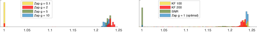
Figure 1: Average rewards obtained using various Q-learning algorithms

In this section we illustrate the performance of the Zap Q-learning algorithm in comparison with existing techniques, on a finance problem that has been studied in prior work [6, 15]. We observe that the Zap algorithm performs very well, despite the fact that some of the technical assumptions made in Section III do not hold.

V-A Finance model

The following finance example is used in [6, 15] to evaluate the performance of their algorithms for optimal stopping. The reader is referred to these references for complete details of the problem set-up.

The Markovian state process considered is the vector of ratios: $X_{n}=(\widetilde{p}_{n-99},\widetilde{p}_{n-98},\ldots,\widetilde{p}_{n})^{\hbox{\it\tiny T}}/\widetilde{p}_{n-100}$, $n\geq 0$, in which $\{\widetilde{p}_{t}:t\in\mathbb{R}\}$ is a geometric Brownian motion (derived from an exogenous price-process). This uncontrolled Markov chain is positive Harris recurrent on the state space ${\sf X}\equiv\mathbb{R}^{100}$, so ${\sf X}$ is not compact. The Markov chain is uniformly ergodic.

The “time to exercise” is modeled as a stopping time $\tau\in{\mathchoice{\mbox{\boldmath$Z$}}{\mbox{\boldmath$Z$}}{\mbox{\boldmath$\scriptstyle Z$}}{\mbox{\boldmath$\scriptscriptstyle Z$}}}^{+}$. The associated expected reward is defined as ${\sf E}[\beta^{\tau}r(X_{\tau})]$, with $r(X_{n})\mathbin{:=}X_{n}(100)=\widetilde{p}_{n}/\widetilde{p}_{n-100}$ and $\beta\in(0,1)$ fixed. The objective of finding a policy that maximizes the expected reward is modeled as an optimal stopping time problem.

The value function is defined to be the infimum (4), with $c\equiv 0$ and ${c}_{{s}}\equiv-r$ (the objective in Section I is to minimize the expected cost, while here, the objective is to maximize the expected reward). The associated Q-function is defined using (5), and the associated optimal policy using (6): $\phi^{*}(x)=\mathbb{I}\{r(x)\geq Q^{*}(x)\}.$

When the Q-function is linearly approximated using (10), for a fixed parameter vector $\theta$, the associated value function can be expressed:

$$h_{\phi^{\theta}}(x) \mathbin{:=}{\sf E}[\beta^{\tau_{\theta}}r(X_{\tau_{\theta}})\mid x_{0}=x]\,,$$ (45)

where,

$$\tau_{\theta} \mathbin{:=}\min\{n\colon\phi^{\theta}(X_{n})=1\}$$ (46)

$$\phi^{\theta}(x) \mathbin{:=}\mathbb{I}\{r(x)\geq Q^{\theta}(x)\}$$

Given a parameter estimate $\theta$ and the initial state $X(0)=x$, the corresponding average reward $h_{\phi^{\theta}}(x)$ was estimated using Monte-Carlo in the numerical experiments that follow.

V-B Approximation & Algorithms

Along with Zap Q-learning algorithm we also implement the fixed point Kalman filter algorithm of [6] to estimate $\theta^{*}$. This algorithm is given by the update equations (20) and (21). The computational as well as storage complexities of the least squares Q-learning algorithm (and its variants) [18] are too high for implementation.

V-C Implementation Details

The experimental setting of [6, 15] is used to define the set of basis functions and other parameters. We choose the dimension of the parameter vector $d=10$, with the basis functions defined in [6]. The objective here is to compare the performances of the fixed point Kalman filter algorithm with the Zap-Q learning algorithm in terms of the resulting average reward (45).

Recall that the step-size for the Zap Q-learning algorithm is given in (25). We set $\gamma_{n}={n^{-0.85}}$ for all implementations of the Zap algorithm, but similar to what is done in [6], we experiment with different choices for $\alpha_{n}$. Specifically, in addition to $\alpha_{n}=n^{-1}$, we let:

$$\alpha_{n}=\frac{g}{b+n}$$ (47)

with $b=1e4$ and experiment with $g=2,5,$ and $10$. In addition, we also implement Zap with $(\alpha_{n}=0.1/n\,,\gamma_{n}=1/n^{0.85})$. Based on the discussion in Section III-C, we expect this choice of step-size sequences to result in infinite asymptotic variance.

In the implementation of the fixed point Kalman filter algorithm, as suggested by the authors, we choose step-size $\alpha_{n}\!=\!1/n$ for the matrix gain update rule in (21), and step-size of the form (47) for the parameter update in (20). Specifically, we let $b=1e4$, and $g=100$ and $200$.

The number of iterations for each of the algorithm is fixed to be $N=2e6$.

V-D Experimental Results

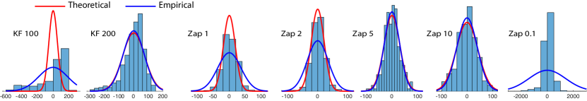
Figure 2: Asymptotic variance for various Q-learning algorithms for optimal stopping in finance

The average reward histogram was obtained by the following steps: We simulate $500$ parallel simulations of each of the algorithms to obtain as many estimates of $\theta^{*}$. Each of these estimates defines a policy $\phi^{\theta_{N}}$ defined in (46). We then estimate the corresponding average reward $h_{\phi^{\theta_{N}}}(x)$ defined in (45), with $X(0)=x=1$.

Along with the average discounted rewards, we also plot the histograms to visualize the asymptotic variance (33), for each of the algorithms. The theoretical values of the covariance matrices $\Sigma^{*}$ and $\Sigma^{G}_{\Theta}$ were estimated through the following steps: The matrices $A(\theta^{*})$ and $\Sigma_{\psi}$ (the limit of the matrix gain used in [6]) were estimated via Monte-Carlo. Estimation of $A(\theta^{*})$ requires an estimate of $\theta^{*}$; this was taken to be $\theta_{N}$ obtained using the Zap-Q algorithm with $\alpha_{n}=n^{-1}$ and $\gamma_{n}=n^{-0.85}$. This estimate of $\theta^{*}$ was also used to estimate the covariance matrix $\Sigma_{\Delta}$ defined in (37) using the batch means method. The matrices $\Sigma^{G}_{\Theta}$ and $\Sigma^{*}$ were then obtained using (34) and (38), respectively.

Fig. 1 contains the histograms of the average rewards obtained using the above algorithms. Fig. 2 contains the histograms of $\sqrt{N}\big{(}\theta_{N}(8)-\theta^{*}(8)\big{)}$ along with a plot of the theoretical prediction.

It was observed that the eigenvalues of the matrix $A(\theta^{*})$ have a wide spread: The condition-number is of the order $10^{4}$. Despite a badly conditioned matrix gain, it is observed in Fig. 1, that the average rewards of the Zap-Q algorithms are better than its competitors. It is also observed that the algorithm is robust to the choice of step-sizes. In Fig. 2 we observe that the asymptotic behavior of the algorithms is close match to the theoretical prediction. Specifically, large variance of Zap-Q with step-size $\alpha_{n}=0.1/n$ confirms that the asymptotic variance is very large (ideally, infinity), if the eigenvalues of the matrix $GA(\theta^{*})>-{\mathchoice{\genfrac{}{}{}{1}{1}{2}}{\genfrac{}{}{}{1}{1}{2}}{\genfrac{}{}{}{3}{1}{2}}{\genfrac{}{}{}{3}{1}{2}}}$.

VI Conclusion

In this paper, we extend the theory for the Zap Q-learning algorithm to a linear function approximation setting, with application to optimal stopping. We prove convergence of the algorithm using ODE analysis, and also observe that it achieves optimal asymptotic variance. The extension of the previous analysis to the current setting is not trivial: Analysis of Zap-Q in the tabular case is much simpler, with lots of special structures, and in general, the theory for convergence of Q-learning algorithms in a function approximation setting does not exist. More importantly, we believe that the ODE analysis obtained in this paper provides important insights into the behavior of the Zap-Q algorithm, even in a function approximation setting. This may be a starting point for analysis of Q-learning algorithms in general function-approximation settings, which is an on-going work.

VII APPENDIX

Proof of Lemma III.2

Based on the definition (29), we have:

$$\|F^{\theta}Q-F^{\theta}Q^{\prime}\| =\beta\|PH^{\theta}Q-PH^{\theta}Q^{\prime}\|$$

$$\leq\beta\|H^{\theta}Q-H^{\theta}Q^{\prime}\|$$

$$\leq\beta\|Q-Q^{\prime}\|\,,$$

where the first inequality follows from the fact that $\|P\|\leq 1$ (with $\|P\|$ being the induced operator norm in $L_{2}(\pi)$). The last inequality is true because:

$$H^{\theta}Q(x)-H^{\theta}Q^{\prime}(x)=S_{\theta}\big{(}Q-Q^{\prime}\big{)}(x)\,,\quad x\in{\sf X}$$

$\sqcap$$\sqcup$

Proof of Lemma III.3

To show result (i), we rewrite $A(\theta)$ as the difference of two matrices, $A(\theta)=A_{NL}(\theta)-A_{L}$, denoting $A_{NL}(\theta)$ to be the part of the matrix that depends on $\theta$ and $A_{L}$ to be the one that is independent of $\theta$:

$$A_{NL}(\theta) \mathbin{:=}{\sf E}[\psi(X_{n})\beta S_{\theta}\psi^{\hbox{\it\tiny T}}(X_{n+1})]$$

$$A_{L} \mathbin{:=}{\sf E}[\psi(X_{n})\psi^{\hbox{\it\tiny T}}(X_{n})]$$

Proving (30) is equivalent to proving:

$$v^{\hbox{\it\tiny T}}A_{NL}(\theta)v-v^{\hbox{\it\tiny T}}A_{L}v\leq(\beta-1)v^{\hbox{\it\tiny T}}\Sigma_{\psi}v,\quad v\in\mathbb{R}^{d}.$$

The proof is easier to follow if we suppose that the vector $v$ is a difference of two parameter vectors, $v=\theta^{1}-\theta^{2}$. Expanding the left hand side of the above inequality:

$$v^{\hbox{\it\tiny T}}A_{NL}(\theta)v =(\theta^{1}-\theta^{2})^{\hbox{\it\tiny T}}{\sf E}\big{[}\psi(X_{n})\beta PH^{\theta}\big{(}Q^{\theta^{1}}(X_{n})-Q^{\theta^{2}}(X_{n})\big{)}\big{]}$$

$$=\beta{\sf E}\big{[}\big{(}Q^{\theta^{1}}(X_{n})-Q^{\theta^{2}}(X_{n})\big{)}PH^{\theta}\big{(}Q^{\theta^{1}}(X_{n})-Q^{\theta^{2}}(X_{n})\big{)}\big{]}.$$

Next, using Cauchy-Schwartz and the fact that $\|P\|_{\pi}\leq 1$,

$$v^{\hbox{\it\tiny T}}A_{NL}(\theta)v \leq\beta\|Q^{\theta^{1}}-Q^{\theta^{2}}\|\|H^{\theta}(Q^{\theta^{1}}-Q^{\theta^{2}})\|$$

$$\leq\beta\|Q^{\theta^{1}}-Q^{\theta^{2}}\|^{2}$$

$$=\beta v^{\hbox{\it\tiny T}}A_{L}v.$$

$$=(\beta-1)v^{\hbox{\it\tiny T}}A_{L}v+v^{\hbox{\it\tiny T}}A_{L}v.$$

Rearranging the terms, and noting that $\Sigma_{\psi}=A_{L}$, the statement of the Lemma follows:

$$v^{\hbox{\it\tiny T}}A(\theta)v =v^{\hbox{\it\tiny T}}A_{NL}(\theta)v-v^{\hbox{\it\tiny T}}A_{L}v$$ (48)

$$\leq(\beta-1)v^{\hbox{\it\tiny T}}\Sigma_{\psi}v$$

Next, for fixed matrix $A(\theta)$ with eigenvalue-eigenvector pair $\lambda_{A}\in\mathbb{C}$, $v=a+bi\in\mathbb{C}^{d}$, we consider

$$v^{*}A(\theta)v=(a^{\hbox{\it\tiny T}}-b^{\hbox{\it\tiny T}}i)A(\theta)(a+bi)=a^{\hbox{\it\tiny T}}A(\theta)a+b^{\hbox{\it\tiny T}}A(\theta)b+[a^{\hbox{\it\tiny T}}A(\theta)b-b^{\hbox{\it\tiny T}}A(\theta)a]i$$

where $v^{*}$ denotes the conjugate transpose of $v$. With $v^{*}A(\theta)v=\lambda_{A}v^{*}v$, it follows that

$$\text{Re}\{\lambda_{A}\}v^{*}v=\text{Re}\{v^{*}A(\theta)v\}=a^{\hbox{\it\tiny T}}A(\theta)a+b^{\hbox{\it\tiny T}}A(\theta)b$$

Let $\lambda_{\psi}>0$ be the largest eigenvalue of $\Sigma_{\psi}$, by the inequality (48), the following relation holds

$$\text{Re}\{\lambda_{A}\}v^{*}v =a^{\hbox{\it\tiny T}}A(\theta)a+b^{\hbox{\it\tiny T}}A(\theta)b$$

$$\leq(\beta-1)\lambda_{\psi}[a^{\hbox{\it\tiny T}}a+b^{\hbox{\it\tiny T}}b]$$

$$=(\beta-1)\lambda_{\psi}v^{*}v$$

Therefore, $\text{Re}\{\lambda_{A}\}$ is negative and bounded above by $(\beta-1)\lambda_{\psi}$. For the last part, $\|A(\theta)^{-1}\|_{F}$ is bounded using an inequality from [5]

$$\|A(\theta)^{-1}\|_{F}\leq\frac{\sqrt{d}}{|{\mathop{\rm det}}A(\theta)|}\Big{(}\frac{\|A(\theta)\|_{F}}{d-1}\Big{)}^{\frac{d-1}{2}}$$ (49)

where $d$ is the dimension. Provided the bound over eigenvalues of $A(\theta)$ and compactness assumption of state space ${\sf X}$, there exists some constant $\ell_{A}$ such that

$$\|A(\theta)^{-1}\|_{F}\leq\frac{\sqrt{d}}{[(1-\beta)\lambda_{\psi}]^{d}}\Big{(}\frac{\ell_{A}}{d-1}\Big{)}^{\frac{d-1}{2}}$$ (50)

The claim of uniform boundedness of $\{A(\theta)^{-1}:\theta\in\mathbb{R}^{d}\}$ then follows. $\blacksquare$

Proof of Lemma III.4

For any two parameter vectors $\theta^{1},\theta^{2}\in\mathbb{R}^{d}$, we have:

$$\|b(\theta^{1})-b(\theta^{2})\| =\|\psi(-FQ^{\theta^{1}}+FQ^{\theta^{2}}+Q^{\theta^{1}}-Q^{\theta^{2}})\|$$

$$\leq\|\psi(FQ^{\theta^{1}}-FQ^{\theta^{2}})\|+\|\psi(Q^{\theta^{1}}-Q^{\theta^{2}})\|$$

$$\leq\beta\|\psi(Q^{\theta^{1}}-Q^{\theta^{2}})\|+\|\psi(Q^{\theta^{1}}-Q^{\theta^{2}})\|$$

$$\leq(1+\beta)\|\psi\|^{2}\|\theta^{1}-\theta^{2}\|.$$

$\blacksquare$

Lemma VII.1

Suppose that $f$ is a bounded function on ${\sf X}$ with zero mean. Then the sequence $\{f(X_{n})\}$ is ODE-friendly, with $\{\varepsilon_{k}\}$ equal to zero, and ${\cal T}_{k}=\hat{f}(X_{k})$, with $\hat{f}$ the solution to Poisson’s equation with forcing function $f$; That is, ${\hat{f}}$ satisfies

$${\hat{f}}(x)=f(x)-\pi(f)+{\sf E}[{\hat{f}}(X_{n+1})|X_{n}=x]\,,x\in{\sf X}\,,$$

where $\pi(f)\mathbin{:=}{\sf E}[f(X)]\,,X\sim\pi$.     $\sqcap$$\sqcup$

Proof:

Let $\hat{f}:{\sf X}\rightarrow\mathbb{R}^{d}$ solve Poisson’s equation:

$${\sf E}[\hat{f}(X_{n+1})-\hat{f}(X_{n})|\mathcal{F}_{n}]=f(X_{n})$$

with the forcing function $f(X_{n})$ in Lemma VII.1. The following decomposition is obtained:

$$f(X_{n}) ={\sf E}[\hat{f}(X_{n+1})-\hat{f}(X_{n})|\mathcal{F}_{n}]$$

$$=\underbrace{{\sf E}[\hat{f}(X_{n+1})|\mathcal{F}_{n}]-\hat{f}(X_{n+1})}_{\text{Martingale difference}}+\underbrace{\hat{f}(X_{n+1})-\hat{f}(X_{n})}_{\text{telescoping}}$$

where $\hat{f}(X_{n})$ is bounded since the forcing function $f(X_{n})$ is bounded [9].     $\sqcap$$\sqcup$

Lemma VII.2

Denote for $n\geq 0$, $M_{\psi,\theta}({n+1})=\psi(X_{n}){\cal S}_{\theta}\psi^{\hbox{\it\tiny T}}(X_{n+1})$. There exists a constant $\ell_{M}<\infty$ such that, with probability one,

$$\|{\sf E}\big{[}M_{\psi,\theta^{1}}({n+1})-M_{\psi,\theta^{2}}({n+1})\mid{\cal F}_{n}\big{]}\|\leq\ell_{M}\|\theta^{1}-\theta^{2}\|$$

$\sqcap$$\sqcup$

Proof:

For $\theta^{1},\theta^{2}$, by Markov property with $X_{n}=x$, we rewrite the term as

$${\sf E}\big{[}\psi(X_{n}){\cal S}_{\theta^{1}}\psi(X_{n+1})^{\hbox{\it\tiny T}}|\mathcal{F}_{n}\big{]}-{\sf E}\big{[}\psi(X_{n}){\cal S}_{\theta^{2}}\psi(X_{n+1})^{\hbox{\it\tiny T}}|\mathcal{F}_{n}\big{]}$$

$$={\sf E}\big{[}\psi(x){\cal S}_{\theta^{1}}\psi(X_{n+1})^{\hbox{\it\tiny T}}|X_{n}=x\big{]}-{\sf E}\big{[}\psi(x){\cal S}_{\theta^{2}}\psi(X_{n+1})^{\hbox{\it\tiny T}}|X_{n}=x\big{]}$$

By Assumption A3, the terminating cost function $c_{s}-1$ is in the span of basis. There exists some constant $\theta_{cs}$ such that

$$c_{s}(y)\equiv\psi^{\hbox{\it\tiny T}}(y)\theta_{cs}+1,\quad\forall y\in{\sf X}.$$

Denote $Z\sim\mathcal{N}(\psi(x),I)$ as the random variable with density $p_{Z}(\cdot)$, we have, for some $\ell_{E}>0$,

$$\|{\sf E}\big{[}\psi(x){\cal S}_{\theta^{1}}\psi(X_{n+1})^{\hbox{\it\tiny T}}|X_{n}=x\big{]}-{\sf E}\big{[}\psi(x){\cal S}_{\theta^{2}}\psi(X_{n+1})^{\hbox{\it\tiny T}}|X_{n}=x\big{]}\|$$

$$\leq{\sf E}\big{[}\|\psi(x)\psi^{\hbox{\it\tiny T}}(X_{n+1})\|\cdot\big{|}\mathbb{I}\{\psi(X_{n+1})^{\hbox{\it\tiny T}}\theta^{1}\leq c_{s}(X_{n+1})\}-\mathbb{I}\{\psi(X_{n+1})^{\hbox{\it\tiny T}}\theta^{2}\leq c_{s}(X_{n+1})\}\big{|}|X_{n}=x\big{]}$$

$$={\sf E}\big{[}\|\psi(x)\psi^{\hbox{\it\tiny T}}(X_{n+1})\|\cdot\big{|}\mathbb{I}\{\psi(X_{n+1})^{\hbox{\it\tiny T}}(\theta^{1}-\theta_{cs})\leq 1\}-\mathbb{I}\{\psi(X_{n+1})^{\hbox{\it\tiny T}}(\theta^{2}-\theta_{cs})\leq 1\}\big{|}|X_{n}=x\big{]}$$

$$=\int\|\psi(x)z^{\hbox{\it\tiny T}}\|\cdot\ell(z|x)\cdot\big{|}\mathbb{I}\{z^{\hbox{\it\tiny T}}(\theta^{1}-\theta_{cs})\leq 1\}-\mathbb{I}\{z^{\hbox{\it\tiny T}}(\theta^{2}-\theta_{cs})\leq 1\}\big{|}p_{Z}(z)dz$$

$$\leq\ell_{E}\int\big{|}\mathbb{I}\{z^{\hbox{\it\tiny T}}(\theta^{1}-\theta_{c})\leq 1\}-\mathbb{I}\{z^{\hbox{\it\tiny T}}(\theta^{2}-\theta_{c})\leq 1\}\big{|}p_{Z}(z)dz$$

$$=\ell_{E}{\sf E}[\big{|}\mathbb{I}\{Z^{\hbox{\it\tiny T}}(\theta^{1}-\theta_{c})\leq 1\}-\mathbb{I}\{Z^{\hbox{\it\tiny T}}(\theta^{2}-\theta_{c})\leq 1\}\big{|}\big{]}$$

As a result, we only need to show that the expectation in the last line is Lipschitz continuous for a Gaussian random variable, for which a bounded derivative of ${\sf E}[\mathbb{I}\{Z^{\hbox{\it\tiny T}}\theta\leq 1\}]$ w.r.t $\theta$ will suffice. For each $\theta$, $Z^{\hbox{\it\tiny T}}\theta$ follows Gaussian distribution $\mathcal{N}(\theta^{\hbox{\it\tiny T}}\psi(x),\theta^{\hbox{\it\tiny T}}\theta)$. Denote ${\sf E}[\mathbb{I}\{Z^{\hbox{\it\tiny T}}\theta\leq 1\}]$ as $m(\theta)$

$$m(\theta)\mathbin{:=}{\sf E}[\mathbb{I}\{Z^{\hbox{\it\tiny T}}\theta\leq 1\}\big{]}=\int_{-\infty}^{1}\frac{1}{\sqrt{2\pi\theta^{\hbox{\it\tiny T}}\theta}}\exp\Big{(}-\frac{1}{2\|\theta\|^{2}}(v-\theta^{\hbox{\it\tiny T}}\psi(x))^{2}\Big{)}dv$$

Applying the change of variable $u=\frac{1}{\sqrt{2\|\theta\|^{2}}}(v-\theta^{\hbox{\it\tiny T}}\psi(x))$, we have

$$m(\theta) =\int_{-\infty}^{\frac{1}{\sqrt{2\|\theta\|^{2}}}(1-\theta^{\hbox{\it\tiny T}}\psi(x))}\frac{1}{\sqrt{2\pi\|\theta\|^{2}}}\exp\big{(}-u^{2}\big{)}du\sqrt{2\|\theta\|^{2}}$$

$$=\frac{1}{\sqrt{\pi}}\int_{-\infty}^{\frac{1}{\sqrt{2\|\theta\|^{2}}}(1-\theta^{\hbox{\it\tiny T}}\psi(x))}\exp\big{(}-u^{2}\big{)}du$$

Its derivative is

$$\frac{d}{d\theta}m(\theta)=[\frac{1}{\sqrt{2\pi}}\frac{-\psi(x)\|\theta\|-(1-\psi(x)^{\hbox{\it\tiny T}}\theta)\cdot\|\theta\|^{-1}\theta}{\|\theta\|^{2}}]\exp\big{(}-\frac{(1-\theta^{\hbox{\it\tiny T}}\psi(x))^{2}}{2\|\theta\|^{2}}\big{)}$$

We observe that

1. If $\|\theta\|\rightarrow\infty$, the exponential term is bounded by 1, and the coefficient before exponential term goes to zero since

   $$\frac{\psi(x)}{\|\theta\|}+\frac{(1-\psi(x)^{\hbox{\it\tiny T}}\theta)}{\|\theta\|^{2}}\rightarrow 0$$

2. $m^{\prime}(\theta)$ also vanishes as $\|\theta\|\rightarrow 0$ since

   $$\big{[}\frac{\psi(x)}{\|\theta\|}+\frac{(1-\psi(x)^{\hbox{\it\tiny T}}\theta)}{\|\theta\|^{2}}\big{]}\exp\big{(}-\frac{(1-\theta^{\hbox{\it\tiny T}}\psi(x))^{2}}{\sqrt{2\|\theta\|^{2}}}\big{)}\rightarrow 0$$

Since the state space ${\sf X}$ is compact, there exists a deterministic bound over $m^{\prime}(\theta)$ that does not depend on $x$. As a result, the objective in Lemma VII.2 is Lipschitz continuous with some deterministic Lipschitz constant $\ell_{M}$.     $\sqcap$$\sqcup$

Lemma VII.3

There is a constant $B_{Z}$ such that the following holds: For any family of zero mean functions $\{f_{\theta}\}$ satisfying for some constants $B_{F}$, $\ell_{F}$,

$$\sup_{x}\|f_{\theta}(x)\| \leq B_{F},$$

$$\sup_{x}\|f_{\theta^{1}}(x)-f_{\theta^{2}}(x)\| \leq\ell_{F}\|\theta^{1}-\theta^{2}\|$$

for all $\theta,\theta^{1},\theta^{2}$, then, there are solutions to corresponding Poisson’s equation, $\{{\hat{f}}_{\theta}\}$, with zero mean, and satisfying

$$\sup_{x}\|{\hat{f}}_{\theta^{1}}(x)-{\hat{f}}_{\theta^{2}}(x)\|\leq B_{Z}\ell_{F}\|\theta^{1}-\theta^{2}\|$$

$\sqcap$$\sqcup$

Proof:

Let $P$ denote transition kernel of the Markov chain, we define the following fundamental kernel $\mathcal{Z}$

$$\mathcal{Z} \mathbin{:=}[I-P+\mathbbm{1}\otimes\pi]^{-1}=\sum_{n=0}^{\infty}[P-\mathbbm{1}\otimes\pi]^{n}=I+\sum_{n=1}^{\infty}[P^{n}-\mathbbm{1}\otimes\pi]$$ (51)

Note that $\hat{f}_{\theta}=\mathcal{Z}f_{\theta}$ solves Poisson’s equation:

$$P\hat{f}_{\theta}=\hat{f}_{\theta}-f_{\theta}$$

Since $\mathcal{Z}:L_{\infty}\rightarrow L_{\infty}$ is a bounded linear operator, we have that for any $x\in{\sf X}$,

$$\|h_{\theta^{1}}(x)-h_{\theta^{2}}(x)\|\leq\|h_{\theta^{1}}-h_{\theta^{2}}\|_{\infty}\leq\|\mathcal{Z}\|_{\infty}\|f_{\theta^{1}}-f_{\theta^{2}}\|_{\infty}\leq\ell_{F}\|\mathcal{Z}\|_{\infty}\|\theta^{1}-\theta^{2}\|$$

where $\|\mathcal{Z}\|_{\infty}$ denotes the induced operator norm.     $\sqcap$$\sqcup$

Proof of Lemma IV.1

Based on (23, 24), the two error sequences in (42) are

$${\cal E}^{\theta}_{n+1} =c(X_{n})\psi(X_{n})-b^{*}+\beta{\cal S}^{c}_{\theta_{n}}{c}_{{s}}(X_{n+1})-\beta\overline{c}_{{s}}(\theta_{n})$$

$${\cal E}^{A}_{n+1} =A_{n+1}-A(\theta_{n})$$

The argument proceeds by decomposing noise sequences into tractable terms, each of which is shown to be ODE-friendly by standard arguments based on solutions to Poisson’s equation [11]. We only present the treatment for ${\cal E}^{A}_{n+1}$ here since same technique can be applied to ${\cal E}^{A}_{n+1}\theta_{n}$ and ${\cal E}_{n+1}^{\theta}$.

Denote for $n\geq 0$,

$$M_{\psi,\theta}({n+1})=\psi(X_{n}){\cal S}_{\theta}\psi^{\hbox{\it\tiny T}}(X_{n+1})$$

For noise sequence $\mathcal{E}_{n+1}^{A}$ in (42b), we have

$${\cal E}^{A}_{n+1}=A_{n+1}-A(\theta_{n}) =\psi(X_{n})\big{[}\beta{\cal S}_{\theta_{n}}\psi(X_{n+1})-\psi(X_{n})\big{]}^{\hbox{\it\tiny T}}-{\sf E}\big{[}\psi(X_{n})[\beta{\cal S}_{\theta_{n}}\psi(X_{n+1})-\psi(X_{n})]^{\hbox{\it\tiny T}}\big{]}$$ (52)

$$=\tilde{A}_{n+1}^{1}+\beta\tilde{A}_{n+1}^{2}+\beta\tilde{A}_{n+1}^{3}$$

where

$$\tilde{A}_{n+1}^{1} =-\psi(X_{n})\psi^{\hbox{\it\tiny T}}(X_{n})+{\sf E}[\psi(X_{n})\psi^{\hbox{\it\tiny T}}(X_{n})]$$

$$\tilde{A}_{n+1}^{2} =M_{\psi,\theta_{n}}({n+1})-{\sf E}[M_{\psi,\theta_{n}}({n+1})\mid{\cal F}_{n}]$$

$$\tilde{A}_{n+1}^{3} ={\sf E}[M_{\psi,\theta_{n}}({n+1})\mid{\cal F}_{n}]-{\sf E}[M_{\psi,\theta_{n}}({n+1})]$$

Lemma VII.1 implies that the sequence $\{\tilde{A}^{1}_{n+1}\}$ is ODE-friendly since it is bounded over state space ${\sf X}$, and has zero mean. $\{\tilde{A}_{n+1}^{2}\}$ is ODE friendly as it is martingale difference sequence with bounded moments.

For $\tilde{A}_{n+1}^{3}$, let $\hat{f}_{\theta}:\Theta\times{\sf X}\rightarrow\mathbb{R}^{d\times d}$ solve Poisson’s equation:

$${\sf E}[\hat{f}_{\theta}(X_{n+1})-\hat{f}_{\theta}(X_{n})|\mathcal{F}_{n}]=f_{\theta}(X_{n})$$

with forcing function $f_{\theta}(X_{n})\mathbin{:=}\tilde{A}^{3}_{n+1}$. The following representation is obtained:

$$f_{\theta_{n}}(X_{n})= {\sf E}[\hat{f}_{\theta_{n}}(X_{n+1})-\hat{f}_{\theta_{n}}(X_{n})|\mathcal{F}_{n}]$$

$$= {\sf E}[\hat{f}_{\theta_{n}}(X_{n+1})|\mathcal{F}_{n}]-\hat{f}_{\theta_{n}}(X_{n+1})+\hat{f}_{\theta_{n}}(X_{n+1})-\hat{f}_{\theta_{n}}(X_{n})$$

$$= \underbrace{{\sf E}[\hat{f}_{\theta_{n}}(X_{n+1})|\mathcal{F}_{n}]-\hat{f}_{\theta_{n}}(X_{n+1})}_{\text{Martingale difference}}+\underbrace{\hat{f}_{\theta_{n+1}}(X_{n+1})-\hat{f}_{\theta_{n}}(X_{n})}_{\text{telescoping}}+\underbrace{\hat{f}_{\theta_{n}}(X_{n+1})-\hat{f}_{\theta_{n+1}}(X_{n+1})}_{\text{perturbation}}$$

which admits the form of being ODE-friendly, provided the perturbation term $\varepsilon_{n}:=\hat{f}_{\theta_{n}}(X_{n+1})-\hat{f}_{\theta_{n+1}}(X_{n+1})$ satisfies

$$\sum_{k=1}^{\infty}\gamma_{k}\|\varepsilon_{k}\|<\infty,\quad a.s..$$

Recall that Lemma VII.2 shows $\tilde{A}_{n+1}^{3}$ is Lipschitz continuous with deterministic Lipschitz constant. Combining this with Lemma VII.3 shows that $\hat{f}_{\theta}(X_{n+1})$ is uniformly Lipschitz continuous w.r.t $\theta$ with Lipschitz constant $B_{Z}\ell_{F}$, which indicates

$$\sum_{k=1}^{\infty}\gamma_{k}\|\varepsilon_{k}\| =\sum_{k=1}^{\infty}\gamma_{k}\|\hat{f}_{\theta_{k}}(X_{k+1})-\hat{f}_{\theta_{k+1}}(X_{k+1})\|\leq\sum_{k=1}^{\infty}\gamma_{k}B_{Z}\ell_{F}\|\theta_{k}-\theta_{k+1}\|$$

$$\leq B_{Z}\ell_{F}\sum_{k=1}^{\infty}\gamma_{k}\alpha_{k}\|\widehat{A}_{k}^{\dagger}\psi(X_{k})(c(X_{k})+\beta\min(c_{s}(X_{k+1}),Q^{\theta_{k}}(X_{k+1}))-Q^{\theta_{k}}(X_{k}))\|$$

which is bounded by the boundedness assumption over $\{\theta_{n}\}$ and the fact that we use projected pseudo-inverse of $\widehat{A}_{n+1}$. $\blacksquare$

Proof of Lemma IV.2

Consider the update rules for $\theta_{n},\widehat{A}_{n}$ in (23) and (24). When both update rules are viewed as over the faster time-scale (that is, with step-size sequence $\{\gamma_{n}\}$), they can be rewritten as [2]:

$$\theta_{n+1}= \theta_{n}+\gamma_{n+1}\big{[}o(1)\big{]}$$ (53)

$$\widehat{A}_{n+1}= \widehat{A}_{n}+\gamma_{n+1}\big{[}A(\theta_{n})-\widehat{A}_{n}+\mathcal{E}^{A}_{n+1}\big{]}$$

where the $o(1)$ term is:

$$o(1)=-\frac{\alpha_{n+1}}{\gamma_{n+1}}\widehat{A}_{n}^{\dagger}\psi(X_{n})\big{[}c(X_{n})+\beta\min(c_{s}(X_{n+1}),Q^{\theta_{n}}(X_{n+1}))-Q^{\theta_{n}}(X_{n})\big{]}$$

It goes to zero provided stability assumption of $\{\theta_{n}\}$ and boundedness of $\widehat{A}_{n}^{\dagger}$. It follows that $\{\theta_{n},\widehat{A}_{n}\}$ converges a.s. to the internally chain transitive invariant set of the following ODE [2]

$$\dot{w}(t) =0$$

$$\dot{\mathcal{A}}(t) =A(w_{t})-\mathcal{A}(t)$$

Which is $\{(\theta,A(\theta)):\theta\in\mathbb{R}^{d}\}$. In other words, $\|\hat{A}_{n}-A(\theta_{n})\|$ converges to 0 a.s.. While the invertibility of $A(\theta)$ has been established in Lemma III.3. $\blacksquare$

Proof of Lemma IV.3

Within time interval $[s,s+T]$, consider the evolution of $\overline{w}_{t_{k}}$ over slow time scale defined by $\{\alpha_{k}\}$, where $t_{k}$ denote the time of $k$-th update of $\theta$.

$$\overline{w}_{t_{k+1}}=\overline{w}_{t_{k}}- \alpha_{k+1}\widehat{A}_{k+1}^{\dagger}\psi(X_{k})\Big{[}c(X_{k})$$

$$+\beta\min(c_{s}(X_{k+1}),\overline{w}_{t_{k}}^{\hbox{\it\tiny T}}\psi(X_{k+1}))-\overline{w}_{t_{k}}^{\hbox{\it\tiny T}}\psi(X_{k})\Big{]}$$

Write it in standard stochastic approximation form and replace $\widehat{A}_{k+1}^{\dagger}$ with $-A(\theta_{k})^{-1}+o(1)$ by Lemma III.3 and IV.2

$$\overline{w}_{t_{k+1}}=\overline{w}_{t_{k}}- \alpha_{k+1}A^{-1}(\overline{w}_{t_{k}})\Big{[}A(\overline{w}_{t_{k}})\overline{w}_{t_{k}}+\beta\overline{c}_{{s}}(\overline{w}_{t_{k}})+b^{*}$$

$$+\mathcal{E}_{k+1}^{A}\overline{w}_{t_{k}}+\mathcal{E}_{k+1}^{\theta}\Big{]}+o(\alpha_{k+1})$$

With the noise terms being

$$\mathcal{E}_{k+1}^{A}\overline{w}_{t_{k}} =A_{k+1}\overline{w}_{t_{k}}-A(\overline{w}_{t_{k}})\overline{w}_{t_{k}}$$

$$\mathcal{E}_{k+1}^{\theta} =c(X_{k})\psi(X_{k})-b^{*}+\beta{c}_{{s}}(X_{k+1})\mathbb{I}{\{Q^{\theta_{k}}(X_{k+1})>{c}_{{s}}(X_{k+1})\}}-\beta\overline{c}_{{s}}(\theta_{k})$$

With them being shown ODE-friendly in Lemma IV.1, the ODE approximation for $\overline{w}_{t}$ follows under the stability assumption of $\theta_{n}$ [13]. $\blacksquare$

Proof of Lemma IV.4

For result in (i), the first relation holds since mapping $b(\cdot)$ is Lipschitz continuous. The sub-sequential limit $w_{t}$ is the solution of the ODE in (43) since the right hand side of (43) is Lipschitz continuous. It is differentiable everywhere within $[0,T]$.

By definition in (26a), $b_{t}=b(w_{t})$ can be written as follows:

$$b_{t} =-A(w_{t})w_{t}-\beta\overline{c}_{{s}}(w_{t})$$ (54)

$$=-{\sf E}\big{[}\psi(X_{n})(\beta\min\big{(}c_{s}(X_{n+1}),Q^{w_{t}}(X_{n+1})\big{)}-Q^{w_{t}}(X_{n}))\big{]}$$

$$={\sf E}\big{[}\psi(X_{n})c^{w_{t}}(X_{n})\big{]}$$

where, for any $w\in\mathbb{R}^{d}$, $c^{w}$ is the cost function that solves the fixed point equation (5) with $\theta^{*}$ replaced by $w$:

$$c^{w}(x)\mathbin{:=}-{\sf E}\big{[}\beta\min(c_{s}(X_{n+1}),Q^{w}(X_{n+1}))\mid X_{n}=x\big{]}+Q^{w}(x),\qquad x\in{\sf X}$$

The cost function $c^{w}$ is Lipschitz in $w$. Therefore it is Lipschitz continuous over $[0,T]$ and absolutely continuous over $[0,T]$ that has derivative almost everywhere. Let $t_{0}$ be a point of differentiability for $c_{t}=c^{w_{t}}$. Both $w_{t}$ and $c_{t}(x)$ (for each $x\in{\sf X}$) are approximated by a line at this time point:

$$w_{t} =w_{t_{0}}+(t-t_{0})v^{w}+o(|t-t_{0}|)$$

$$c_{t}(x) =c_{t_{0}}(x)+(t-t_{0})v^{c}(x)+o(|t-t_{0}|),\quad t\sim t_{0}$$

where $v^{w},v^{c}(x)$ are the respective derivatives. The assertion

$$v^{c}(x)=-{\sf E}[\beta{\cal S}_{w_{t_{0}}}\psi(X_{n+1})^{\hbox{\it\tiny T}}-\psi(X_{n})^{\hbox{\it\tiny T}}\mid X_{n}=x]v^{w}$$ (55)

will then imply the statement of the Lemma.

Denote $L_{t}^{c}=c_{t_{0}}+(t-t_{0})v^{c}$, $L_{t}^{w}=w_{t_{0}}+(t-t_{0})v^{w}$. For each $t$, we have:

$$L^{c}_{t}(x)= -{\sf E}[\beta\min(c_{s}(X_{n+1}),Q^{L^{w}_{t}}(X_{n+1}))-Q^{L^{w}_{t}}(X_{n})\mid X_{n}=x]$$

$$= -{\sf E}[\beta{\cal S}_{L^{w}_{t}}Q^{L^{w}_{t}}(X_{n+1})+\beta{\cal S}^{c}_{L^{w}_{t}}c_{s}(X_{n+1})-Q^{L^{w}_{t}}(X_{n})\mid X_{n}=x]$$

$$\geq -{\sf E}[\beta{\cal S}_{w_{t_{0}}}Q^{L^{w}_{t}}(X_{n+1})+\beta{\cal S}^{c}_{w_{t_{0}}}c_{s}(X_{n+1})-Q^{L^{w}_{t}}(X_{n})\mid X_{n}=x]$$

$$= c_{t_{0}}(x)-(t-t_{0}){\sf E}[\beta{\cal S}_{w_{t_{0}}}\psi(X_{n+1})^{\hbox{\it\tiny T}}-\psi(X_{n})^{\hbox{\it\tiny T}}\mid X_{n}=x]v^{w}$$

The above inequality is true for both $t>t_{0}$ and $t<t_{0}$. For $t\sim t_{0}$, it follows that the inequality becomes an equality, and therefore (55) holds. The ODE (44) for $b_{t}$ holds by replacing $w_{t}$ with $b_{t}$ in (43) using the above derivative. $\blacksquare$

References

- [1] D. Bertsekas and J. N. Tsitsiklis. Neuro-Dynamic Programming. Atena Scientific, Cambridge, Mass, 1996.
- [2] V. S. Borkar. Stochastic Approximation: A Dynamical Systems Viewpoint. Hindustan Book Agency and Cambridge University Press (jointly), Delhi, India and Cambridge, UK, 2008.
- [3] V. S. Borkar and S. P. Meyn. The ODE method for convergence of stochastic approximation and reinforcement learning. SIAM J. Control Optim., 38(2):447–469, 2000. (also presented at the IEEE CDC, December, 1998).
- [4] S. Chen, A. M. Devraj, A. Bušić, and S. P. Meyn. Zap q-learning for optimal stopping time problems. arXiv preprint arXiv, 2019.
- [5] G. Cheng. Note on some upper bounds for the condition number. JOURNAL OF MATHEMATICAL INEQUALITIES, 8(2):369–374, 2014.
- [6] D. Choi and B. Van Roy. A generalized Kalman filter for fixed point approximation and efficient temporal-difference learning. Discrete Event Dynamic Systems: Theory and Applications, 16(2):207–239, 2006.
- [7] A. M. Devraj and S. Meyn. Zap Q-learning. In Advances in Neural Information Processing Systems, pages 2235–2244, 2017.
- [8] A. M. Devraj and S. P. Meyn. Fastest convergence for Q-learning. ArXiv e-prints, July 2017.
- [9] S. P. Meyn and R. L. Tweedie. Markov chains and stochastic stability. Cambridge University Press, Cambridge, second edition, 2009. Published in the Cambridge Mathematical Library. 1993 edition online.
- [10] A. Nedic and D. Bertsekas. Least squares policy evaluation algorithms with linear function approximation. Discrete Event Dynamic Systems: Theory and Applications, 13(1-2):79–110, 2003.
- [11] A. Shwartz and A. Makowski. On the Poisson equation for Markov chains: existence of solutions and parameter dependence. Technical Report, Technion—Israel Institute of Technology, Haifa 32000, Israel., 1991.
- [12] R. S. Sutton. Learning to predict by the methods of temporal differences. Mach. Learn., 3(1):9–44, 1988.
- [13] V. B. Tadic and S. P. Meyn. Asymptotic properties of two time-scale stochastic approximation algorithms with constant step sizes. In Proceedings of the 2003 American Control Conference, 2003., volume 5, pages 4426–4431. IEEE, 2003.
- [14] J. N. Tsitsiklis and B. Van Roy. An analysis of temporal-difference learning with function approximation. IEEE Trans. Automat. Control, 42(5):674–690, 1997.
- [15] J. N. Tsitsiklis and B. Van Roy. Optimal stopping of Markov processes: Hilbert space theory, approximation algorithms, and an application to pricing high-dimensional financial derivatives. IEEE Trans. Automat. Control, 44(10):1840–1851, 1999.
- [16] C. J. C. H. Watkins. Learning from Delayed Rewards. PhD thesis, King’s College, Cambridge, Cambridge, UK, 1989.
- [17] C. J. C. H. Watkins and P. Dayan. -learning. Machine Learning, 8(3-4):279–292, 1992.
- [18] H. Yu and D. P. Bertsekas. Q-learning algorithms for optimal stopping based on least squares. In 2007 European Control Conference (ECC), pages 2368–2375. IEEE, 2007.