Investigation of the Outburst Activity of the Black Hole Candidate GRS 1739-278

Аннотация

We have performed a joint spectral and timing analysis of the outburst of GRS 1739-278 in 2014 based on Swift and INTEGRAL data. We show that during this outburst the system exhibited both intermediate states: hard and soft. Peaks of quasi-periodic oscillations (QPOs) in the frequency range 0.1-5 Hz classified as type-C QPOs have been detected from the system. Using Swift/BAT data we show that after the 2014 outburst the system passed to the regime of mini-outburst activity: apart from the three mini-outbursts mentioned in the literature, we have detected four more mini-outbursts with a comparable ($\sim$20 mCrab) flux in the hard energy band (15-50 keV). We have investigated the influence of the accretion history on the outburst characteristics: the dependence of the peak flux in the hard energy band in the low/hard state on the time interval between the current and previous peaks has been found (for the outbursts during which the system passed to the high/soft state).
Keywords: X-ray novae, black holes, accretion, GRS 1739-278.

1 INTRODUCTION

During outbursts the transient systems with black hole candidates exhibit several characteristic states. The hardness-intensity and hardness-rms diagrams, on which the systems, as a rule, exhibit characteristic dependences, are used for their classification (Grebenev et al. 1993; Tanaka and Shibazaki 1996; Remillard and McClintock 2006; Belloni 2010; Belloni and Motta 2016). Initially, two states of such systems were detected: low/hard and high/soft (see Remillard and McClintock (2006) and references therein). According to the most popular accretion flow model, in such systems it is believed that the accretion disk in the low/hard state is truncated at a large inner radius, while the region between the disk and the compact object is filled with an optically thin hot plasma, a corona, which makes a major contribution to the source’s emission in the form of a power law with a high-energy cutoff. As the outburst develops, the inner radius of the accretion disk decreases and in the high/soft state the accretion disk makes a major contribution to the system’s emission (Grebenev et al. 1997; Gilfanov 2010).

Subsequently, it was found that between these well-defined states the system could be in transition ones, whose established classification is currently absent (Remillard and McClintock 2006; Belloni and Motta 2016). In this paper we used the classification from Belloni and Motta (2016), according to which the source exhibits hard and soft intermediate states. These states are characterized by both thermal and power-law components in the source’s energy spectrum, but they do not differ greatly from the viewpoint of their spectral characteristics. Nevertheless, there are several distinctive features of these states. In the hard intermediate (and low/hard) state peaks of type C quasi-periodic oscillations (QPOs) and broadband noise at low frequencies with a fractional rms of both components of tens of percent are often observed in the source’s power spectrum. Type-B QPOs, which, as a rule, have a fractional rms of a few percent, and weak (rms < 10%), frequency-dependent noise at low frequencies are detected in the soft intermediate state (Belloni and Motta 2016). The QPO frequency has inverse (type C) and direct (type B) dependences on the flux in the power-law component (Motta et al. 2011). The most popular QPO model is based on the Lense-Thirring precession of a hot corona near the compact object (Ingram et al. 2009), but there is no full physical picture for the formation of QPOs of different types. In the low/hard and hard intermediate states the systems with black hole candidates are observed in the radio band. During the transition to the soft intermediate state the system crosses the so-called "jet line"  and ceases to radiate in the radio band (Remillard and McClintock 2006; Belloni 2010). Thus, an investigation of the intermediate states is required for a more detailed study of the physical processes responsible for the formation of QPOs and jets.

It is believed that during an outburst the system must pass from the low/hard to high/soft state and back, exhibiting the intermediate states and a characteristic "q"  shape on the hardness-intensity diagram (Belloni and Motta 2016). However, many sources with black hole candidates exhibit the so-called failed outbursts, when the system does not reach the high/soft state (Ferrigno et al. 2012, 2014a; Del Santo et al. 2015; Mereminskiy et al. 2017).

The same system can exhibit both types of outbursts (Motta et al. 2010; Furst et al. 2015; Mereminskiy et al. 2017), with the same type of outbursts occurring at peak luminosities differing by tens of times. For example, in GRS 1739-278 the transition to the high/soft state was observed both during bright outbursts, when the peak flux reached 300 mCrab (15-50 keV), and mini-outbursts with a peak flux of 40 mCrab (15-50 keV) (Yan and Yu 2017). Different types of outbursts occur at close peak luminosities - a failed outburst at a peak flux of 30 mCrab in the 15- 50 keV energy band was detected in the same system GRS 1739-278 (Mereminskiy et al. 2017).

At present, there is no full understanding of what physical conditions are necessary for the system’s transition from the low/hard to high/soft state, but it is clear that not only the change in accretion rate is responsible for this process. A hysteresis behavior is observed on the hardness-intensity diagram even within one full-fledged outburst of the source, i.e., the transition from the hard state to the soft one occurs at luminosities greater than the luminosity during the transition from the soft state to the hard one by several (or even tens of) times. The corona size (Homan et al. 2001), the accretion disk size (Smith et al. 2001), the evolution history of the inner accretion disk radius (Zdziarski et al. 2004), and the accretion disk mass (Yu et al. 2004; Yu and Yan 2009) are considered as additional parameters. Yu et al. (2007) and Wu et al. (2010) found a correlation between the luminosity at which the transition from the low/hard to high/soft state occurs and the peak luminosity in the high/soft state, based on which they put forward the idea about the influence of the accretion disk mass on the outburst evolution, and a correlation between the peak flux in the low/hard state and the time interval between the current and previous peak fluxes in the low/hard state. Based on these dependences, the authors hypothesized that the peak luminosity in the low/hard state is also determined by the mass of the accretion disk accumulated between outbursts. Yu et al. (2004, 2009) used mostly low-mass systems with neutron stars, which accounted for about 70% of the samples, to construct the relationship between the luminosity of the transition from the low/hard to high/soft state and the peak luminosity in the high/soft state. In contrast, the correlation between the peak flux in the low/hard state and the time interval between the current and previous peak fluxes in the low/hard state was found only for one system, GX 339-4 (based on eight outbursts detected from 1991 to 2006), and requires a further confirmation based on data for the outbursts from 2006 to 2018. Thus, an investigation of transient systems exhibiting several outbursts is required to develop a physical model for the outbursts of binary systems with black hole candidates, which allows the evolution of binary parameters from outburst to outburst to be measured. GRS 1739-278 belongs to such sources.

1.1 GRS 1739-278 

The X-ray source GRS 1739-278 was discovered by the SIGMA coded-mask telescope onboard the GRANAT observatory on March 18, 1996 (Paul et al. 1996). The peak flux from the source during the first recorded outburst was $\sim 800-1000$ mCrab in the 2-10 keV energy band (Borozdin et al. 1998). The corresponding radio source was detected by Durouchoux et al. (1996). During the 1996 outburst the system passed from the low/hard to high/soft state (Borozdin et al. 1998). QPO peaks at 5 Hz were detected in the source (Borozdin and Trudolyubov 2000). From the shape of the power spectrum and the total fractional rms it can be concluded that the system was recorded in the soft intermediate state and the recorded QPOs are type-B ones.

The second outburst was recorded by the Swift/BAT monitor on March 9, 2014 (Krimm et al. 2014). A spectral analysis of this outburst based on Swift/XRT data was performed by Yu and Yan (2017) and Wang et al. (2018). They showed that during the outburst the system passed from the low/hard to high/soft state through the intermediate one, but no detailed analysis of the intermediate state was made. At the outburst onset (March 19, 2014) the system was also recorded by the INTEGRAL observatory. According to the analysis of these data, the source was recorded up to energies of $\sim 200$ keV, while the energy spectrum was fitted by a power law with a cutoff with the following parameters: a photon index $\Gamma=1.4\pm 2$ and a cutoff energy $E_{cut}=90^{+40}_{-20}$ keV (Filippova et al. 2014b). The source was observed by the NuSTAR observatory (Miller et al. 2015) 17 days after the outburst onset (March 26, 2014). A spectral analysis of the NuSTAR data showed that the system continued to be in the low/hard state. The reflected component of the hard emission presumably associated with an accretion disk whose inner radius must reach the innermost stable orbit was observed in the source’s spectrum, but the disk component itself was not recorded in the spectrum. Mereminskiy et al. (2019) performed a detailed timing analysis of the NuSTAR data, based on which QPOs at frequencies 0.3-0.7 Hz were detected in the variability power spectrum for GRS 1739-278. Based on data from the MAXI monitor, Wang et al. (2018) showed that the system passed back from the high/soft to low/hard state in November-December 2014.

Two mini-outbursts (the peak flux in the 15-50 keV energy band was $\sim 40$ mCrab) were detected from the system 200 days after this outburst. A spectral analysis of the Swift/XRT data showed that during these mini-outbursts the system passed from the low/hard to high/soft state and returned back to the low/hard one (Yu and Yan 2017).

The next outburst from the source was detected in September 2016 (Mereminskiy et al. 2016). During this outburst the peak flux in the 20-60 keV energy band was $\sim 30$ mCrab. Based on our analysis of the INTEGRAL and Swift data, it was shown that during the outburst the system was in the low/hard state and exhibited no transition to the high state. i.e., the outburst turned out to be a failed one (Mereminskiy et al. 2017). Some softening of the spectrum was recorded, i.e., the photon index increased from 1.73 at the outburst onset to 1.86 at the peak flux, with the power law having been observed up to energies $\sim 150$ keV without cutoffs; no contribution to the emission from the accretion disk was recorded.

In this paper for the first time we have performed a simultaneous study of the spectral evolution and temporal variability of the system over the entire 2014 outburst, which has allowed the source’s intermediate states to be classified in detail, made a comparative analysis of the system’s behavior in all of the outbursts detected to date, and investigated the system’s behavior between outbursts.

2 OBSERVATIONS

2.1 Swift Data

GRS 1739-278 during the 2014 outburst was observed by the Swift/XRT telescope in the windowed timing mode (Burrows et al. 2005) from March 20, 2014 (MJD 56736) to November 1, 2014 (MJD 56962), i.e., the observations were begun on the 11th day after the outburst onset. A total of 39 observations with ObsID 000332030XY were carried out; below we will use the last two digits to denote the observation number.

The Swift/XRT light curves and spectra of the source were obtained using an online repository (Evans et al. 2007). Events with grade 0 were selected to analyze the energy spectra. The source’s spectra were investigated in the 0.8-10 keV energy band, because at energies below 0.8 keV the response matrix is known inaccurately due to instrumental effects. The spectra obtained through the online repository by adding the counts in different bins were brought to the form in which there were at least 100 counts per energy channel with the grppha utility. This allowed the $\chi^{2}$ statistic to be used in fitting the spectra in the Xspec package (Arnaud 1996). Instrumental features at energies of 1.8 and 2.3 keV were detected in several spectra (marked in Table 1 by $\dagger$). Therefore, when fitting these data, we, following the recommendations given at the mentioned link, used the gain command in the Xspec package, which modifies the response matrix by shifting the energies at which it was determined. The offset parameters are given in Table 2. Deviations of the data from the model at energies below 1 keV were also observed in several spectra (marked in Table 1 by $\star$). This feature of the spectrum is related to the position of the source’s image on the telescope’s detector. Using the telescope’s response matrix dependent on the source’s position on the detector (swxwt0s6psf1_20131212v001.rmf) allowed the quality of the data fit at low energies to be improved.

To construct the light curves, we used the 0.5-10 keV energy band, events with grade 0-2, the data were averaged over one observation. The typical exposure time for XRT observations was $\sim 1-2$ ks (see Table 1). The light curves used for our Fourier analysis were constructed in the 0.5-10, 0.5-3, and 3-10 keV energy bands with a time resolution of 0.01 s.

The Swift/BAT light curve of the source was retrieved from the online database of light curves (Krimm et al. 2013).

2.2 INTEGRAL Data

We also used the data from the JEM-X and ISGRI/IBIS telescopes onboard the INTEGRAL observatory (Winkler et al. 2003) processed with the HEAVENS service (Walter et al. 2010). These data in combination with the quasi-simultaneous Swift/XRT spectral data were used to construct the source’s broadband spectra in the energy range 0.8-200 keV. When fitting the spectra, we took into account the systematic errors of 1 and 3% for the ISGRI and JEM - X instruments, respectively. The times and exposures of observations for the broadband spectra are given in Table 3.

Таблица 1: Parameters of the best-fit models for the XRT energy spectra

$ID^{a}$	MJD- -56000b	Exp. XRTc s	$N_{H}^{d}$, $10^{22}$cm-2	$\Gamma^{e}$	$T_{in}$, keV f	$R_{in}cos^{-1/2}(i)$, km g	Fluxh	$f_{po}^{j}$	$\chi_{N}^{2}/dof$
$01$	736	$79$	$1.51_{-0.63}^{+0.67}$	$1.24_{-0.36}^{+0.37}$	-	-	$1.57_{-0.29}^{+0.13}$	100	$0.31/7$
$02$	$741$	$2067$	$1.64\pm 0.04$	$1.38\pm 0.03$	-	-	$3.49\pm 0.04$	100	$1.09/459$
$03$	742	$1924$	$1.65\pm 0.03$	$1.38\pm 0.02$	-	-	$4.53\pm 0.04$	100	$1.06/496$
			$2.08_{-0.1}^{+0.11}$	$1.5$	$0.24_{-0.03}^{+0.02}$	$196.05_{-52.37}^{+70.17}$	$4.44_{-0.04}^{+0.03}$	$89\pm 5$	$1.11/495$
			$2.96\pm 0.09$	$1.8$	$0.18\pm 0.01$	$1378.65_{-198.48}^{+235.78}$	$4.2\pm 0.03$	$51\pm 4$	$1.64/495$
$04^{\dagger}$	747	$2463$	$1.82_{-0.06}^{+0.08}$	$2.05_{-0.04}^{+0.08}$	-	-	$7.29_{-0.08}^{+0.07}$	$100$	$1.3/598$
			$1.52_{-0.02}^{+0.08}$	$1.5$	$0.79_{-0.06}^{+0.04}$	$15.7_{-0.73}^{+3.94}$	$7.87_{-0.11}^{+0.06}$	$82\pm 4$	$1.28/597$
			$1.74_{-0.06}^{+0.08}$	$1.8$	$0.65_{-0.09}^{+0.05}$	$19.22_{-3.96}^{+6.33}$	$7.62_{-0.1}^{+0.03}$	$90\pm 5$	$1.27/597$
			$1.9_{-0.07}^{+0.09}$	$2$	$0.51_{-0.06}^{+0.05}$	$25.76_{-10.15}^{+12.89}$	$7.41_{-0.23}^{+0.03}$	$94\pm 4$	$1.28/597$
$05^{\dagger}$	751	$1832$	$1.57_{-0.07}^{+0.08}$	$1.88\pm 0.05$	-	-	$6.76_{-0.05}^{+0.06}$	100	$1.17/552$
			$1.37\pm 0.06$	$1.5$	$0.76_{-0.06}^{+0.1}$	$12.72_{-1.51}^{+1.98}$	$7.17_{-0.14}^{+0.05}$	$88\pm 5$	$1.18/551$
			$1.62_{-0.1}^{+0.07}$	$1.8$	$0.55_{-0.1}^{+0.15}$	$18.49_{-6.13}^{+13.25}$	$6.87_{-0.2}^{+0.03}$	$96\pm 4$	$1.17/551$
			$1.85_{-0.07}^{+0.1}$	$2$	$0.26_{-0.03}^{+0.1}$	$143.63_{-71.44}^{+135.22}$	$6.62_{-0.08}^{+0.04}$	$93\pm 7$	$1.18/551$
$06$	757	$1811$	$2.26\pm 0.03$	$2.25\pm 0.02$	-	-	$10.67_{-0.08}^{+0.07}$	100	$1.43/496$
			$1.74\pm 0.03$	$1.5$	$1.12\pm 0.04$	$14.24_{-0.85}^{+0.94}$	$10.56_{-0.11}^{+0.07}$	$53\pm 4$	$1.28/495$
			$1.85\pm 0.03$	$1.8$	$1.13\pm 0.05$	$12.09_{-0.84}^{+0.97}$	$10.51\pm 0.1$	$66\pm 6$	$1.25/495$
			$1.95\pm 0.03$	$2$	$1.21_{-0.07}^{+0.06}$	$9.21_{-0.68}^{+0.81}$	$10.46_{-0.10}^{+0.09}$	$75\pm 8$	$1.25/495$
$07$	761	$1612$	$2.15\pm 0.03$	$2.11\pm 0.02$	-	-	$8.35_{-0.05}^{+0.06}$		$1.53/514$
			$2.15_{-0.04}^{+0.05}$	$1.5$	$0.61\pm 0.02$	$41.96_{-4.21}^{+4.7}$	$8.9_{-0.1}^{+0.05}$	$70\pm 2$	$1.13/513$
			$2.31_{-0.05}^{+0.06}$	$1.8$	$0.49\pm 0.02$	$62.57_{-9.27}^{+10.74}$	$8.68_{-0.08}^{+0.05}$	$78\pm 3$	$1.1/513$
			$2.43\pm 0.07$	$2$	$0.4_{-0.02}^{+0.03}$	$97.64_{-20.61}^{+24.37}$	$8.47_{-0.1}^{+0.03}$	$82\pm 4$	$1.21/513$
$08^{\star}$	764	$808$	$2.27\pm 0.05$	$2.28\pm 0.03$	-	-	$10.11_{-0.10}^{+0.11}$	1 00	$1.36/366$
			$1.69\pm 0.04$	$1.5$	$1.17\pm 0.06$	$13.15_{-1.07}^{+1.23}$	$9.91_{-0.2}^{+0.11}$	$48\pm 7$	$1.16/365$
			$1.79\pm 0.05$	$1.8$	$1.2\pm 0.07$	$11.27_{-0.94}^{+1.15}$	$9.86_{-0.21}^{+0.16}$	$60\pm 10$	$1.16/365$
			$1.89\pm 0.05$	$2$	$1.28_{-0.09}^{+0.08}$	$9.13_{-0.73}^{+0.89}$	$9.80_{-0.14}^{+0.17}$	$67\pm 12$	$1.16/365$
$09^{\dagger}$	771	$1872$	$1.75_{-0.11}^{+0.1}$	$2.08\pm 0.08$	-	-	$6.14_{-0.11}^{+0.07}$	100	$1.14/504$
			$1.4_{-0.09}^{+0.07}$	$1.5$	$0.84_{-0.07}^{+0.12}$	$12.87_{-2.89}^{+2.9}$	$6.57_{-0.14}^{+0.09}$	$81\pm 7$	$1.14/503$
			$1.58_{-0.09}^{+0.1}$	$1.8$	$0.73_{-0.1}^{+0.16}$	$12.53_{-4.37}^{+6.32}$	$6.39_{-0.18}^{+0.07}$	$90\pm 8$	$1.14/503$
			$1.74_{-0.08}^{+0.1}$	$2$	$0.63_{-0.15}^{+0.29}$	$11.57_{-8.42}^{+13.53}$	$6.21_{-0.19}^{+0.04}$	$96\pm 7$	$1.14/503$
$10^{\star}$	776	$1507$	$2.73\pm 0.04$	$2.22\pm 0.02$	-	-	$16.94_{-0.12}^{+0.1}$	100	$1.37/525$
			$2.32\pm 0.04$	$2$	$1.42\pm 0.06$	$9.53_{-0.52}^{+0.57}$	$16.45_{-0.14}^{+0.16}$	$68\pm 9$	$1.09/524$
			$2.51_{-0.06}^{+0.05}$	$2.4$	$1.85_{-0.05}^{+0.06}$	$6.05_{-0.6}^{+0.58}$	$16.26_{-0.26}^{+0.1}$	$66\pm 9$	$1.12/524$
			$1.8\pm 0.02$	-	$1.72\pm 0.02$	$10.09_{-0.23}^{+0.24}$	$15.53_{-0.13}^{+0.09}$	0	$1.64/525$
$11^{\star\dagger}$	781	$1922$	$2.37_{-0.09}^{+0.13}$	$1.72_{-0.03}^{+0.08}$	-	-	$27.3_{-0.41}^{+0.34}$	100	$1.74/525$
			$1.92_{-0.05}^{+0.09}$	$2$	$1.45_{-0.06}^{+0.03}$	$15.95_{-1.49}^{+1.6}$	$19.76_{-0.3}^{+0.22}$	$11\pm 7$	$1.11/524$
			$2.02_{-0.18}^{+0.11}$	$2.4$	$1.46_{-0.08}^{+0.07}$	$16.07_{-1.91}^{+1.39}$	$19.63_{-0.32}^{+0.27}$	$11\pm 8$	$1.11/524$
			$1.81_{-0.06}^{+0.12}$	-	$1.49_{-0.07}^{+0.05}$	$15.58_{-1.24}^{+1.87}$	$19.55_{-0.76}^{+0.18}$	0	$1.12/525$
$12$	786	$1868$	$2.38\pm 0.03$	$2.3\pm 0.02$	-	-	$8.64_{-0.05}^{+0.06}$	100	$1.18/495$
			$2.04\pm 0.03$	$2$	$1.14\pm 0.06$	$9.73_{-0.72}^{+0.86}$	$8.49\pm 0.08$	$74\pm 6$	$0.99/494$
			$2.25\pm 0.04$	$2.4$	$1.70_{-0.06}^{+0.08}$	$4.2_{-0.58}^{+0.54}$	$8.36_{-0.13}^{+0.04}$	$77\pm 9$	$1.04/494$
			$1.53\pm 0.02$	-	$1.58\pm 0.02$	$8.4_{-0.19}^{+0.2}$	$7.83_{-0.06}^{+0.05}$	0	$1.97/495$

Table 1 (Cont.)

$ID^{a}$	MJD- -56000b	Exp. XRTc s	$N_{H}^{d}$, $10^{22}$cm-2	$\Gamma^{e}$	$T_{in}$, keV f	$R_{in}cos^{-1/2}(i)$, km g	Fluxh	$f_{po}^{j}$	$\chi_{N}^{2}/dof$
$13^{\star}$	791	$1887$	$2.34\pm 0.03$	$2.34\pm 0.02$	-	-	$7.67_{-0.07}^{+0.05}$	100	$1.16/497$
			$1.96\pm 0.03$	$2$	$1.13\pm 0.05$	$9.76_{-0.66}^{+0.77}$	$7.55_{-0.08}^{+0.07}$	$71\pm 6$	$0.99/496$
			$2.12\pm 0.04$	$2.4$	$1.58\pm 0.05$	$4.88^{+0.47}_{-0.50}$	$7.37^{+0.04}_{-0.08}$	$78\pm 9$	$1.02/496$
			$1.48\pm 0.02$	-	$1.55\pm 0.02$	$8.27\pm 0.19$	$6.96_{-0.07}^{+0.04}$	0	$1.99/497$
$14^{\star\dagger}$	796	$2098$	$2.85_{-0.07}^{+0.09}$	$2.27_{-0.03}^{+0.11}$	-	-	$9.67_{-0.09}^{+0.07}$	100	$1.43/542$
			$2.09_{-0.08}^{+0.07}$	$2$	$1.25\pm 0.05$	$11.74_{-1.62}^{+0.64}$	$8.31_{-0.16}^{+0.07}$	$43\pm 10$	$1.09/541$
			$2.34\pm 0.09$	$2.4$	$1.28\pm 0.07$	$10.65_{-0.99}^{+1.59}$	$8.17_{-0.14}^{+0.08}$	$54\pm 10$	$1.09/541$
			$1.59_{-0.01}^{+0.09}$	-	$1.42_{-0.04}^{+0.06}$	$10.68_{-0.82}^{+0.79}$	$7.66\pm 0.07$	0	$1.33/542$
$15$	801	$1988$	$2.46\pm 0.03$	$2.39\pm 0.02$	-	-	$8.68_{-0.06}^{+0.07}$	100	$1.34/472$
			$2.01\pm 0.03$	$2$	$1.16\pm 0.05$	$10.86_{-0.65}^{+0.75}$	$8.48_{-0.10}^{+0.08}$	$65\pm 6$	$1.06/471$
			$2.22\pm 0.05$	$2.4$	$1.48_{-0.04}^{+0.05}$	$6.06_{-0.56}^{+0.53}$	$8.36_{-0.12}^{+0.04}$	$73\pm 10$	$1.08/471$
			$1.57\pm 0.02$	-	$1.52\pm 0.02$	$9.31_{-0.22}^{+0.23}$	$7.87_{-0.06}^{+0.05}$	0	$1.81/472$
$16^{\star}$	806	$1889$	$2.29\pm 0.03$	$2.35\pm 0.02$	-	-	$6.74_{-0.05}^{+0.04}$	100	$1.12/524$
			$2.01\pm 0.03$	$2$	$0.92\pm 0.05$	$12.82_{-1.13}^{+1.33}$	$6.76_{-0.06}^{+0.04}$	$78\pm 4$	$1.05/523$
			$2.25\pm 0.03$	$2.4$	$1.72_{-0.14}^{+0.24}$	$2.28_{-0.78}^{+0.69}$	$6.65_{-0.16}^{+0.03}$	$92\pm 8$	$1.11/523$
			$1.43$	-	$1.52$	$8.08$	$6.05$	0	$3.08/524$
$17^{\star\dagger}$	811	$2045$	$3.13_{-0.39}^{+0.15}$	$2.29_{-0.03}^{+0.05}$	-	-	$10.6\pm 0.12$	100	$1.77/504$
			$2.0_{-0.11}^{+0.07}$	$2$	$1.25_{-0.04}^{+0.08}$	$13.28_{-1.55}^{+1.06}$	$8.69_{-0.26}^{+0.16}$	$29\pm 7$	$1.11/503$
			$2.19_{-0.12}^{+0.07}$	$2.4$	$1.26_{-0.05}^{+0.06}$	$12.72_{-1.26}^{+1.28}$	$8.61_{-0.13}^{+0.08}$	$37\pm 13$	$1.12/503$
			$1.66_{-0.02}^{+0.09}$	-	$1.42_{-0.07}^{+0.04}$	$11.31_{-0.67}^{+1.27}$	$8.37_{-0.32}^{+0.04}$	0	$1.23/504$
$19^{\star}$	823	$2355$	$2.0\pm 0.03$	$2$	$1.29\pm 0.03$	$9.94_{-0.3}^{+0.32}$	$6.7_{-0.04}^{+0.06}$	$41\pm 5$	$1.07/519$
			$2.15\pm 0.05$	$2.4$	$1.4\pm 0.02$	$8.23\pm 0.28$	$6.64_{-0.06}^{+0.05}$	$47\pm 7$	$1.12/519$
			$1.72\pm 0.02$	-	$1.46\pm 0.01$	$9.22_{-0.17}^{+0.18}$	$6.43_{-0.04}^{+0.03}$	0	$1.43/520$
$20^{\dagger}$	826	$1922$	$2.65_{-0.11}^{+0.03}$	$2.58_{-0.08}^{+0.07}$	-	-	$6.76_{-0.07}^{+0.05}$	100	$1.22/503$
			$1.82_{-0.03}^{+0.07}$	$2$	$1.08_{-0.06}^{+0.04}$	$11.3_{-0.95}^{+1.89}$	$6.52_{-0.14}^{+0.06}$	$64\pm 11$	$1.11/502$
			$2.14_{-0.03}^{+0.1}$	$2.4$	$1.12\pm 0.07$	$9.49_{-1.49}^{+1.39}$	$6.35_{-0.09}^{+0.07}$	$76\pm 12$	$1.09/502$
			$1.11_{-0.06}^{+0.04}$	-	$1.48_{-0.02}^{+0.07}$	$8.13_{-0.74}^{+0.57}$	$5.8_{-0.15}^{+0.05}$	0	$1.75/503$
$21^{\dagger}$	831	$826$	$2.95_{-0.39}^{+0.29}$	$2.65\pm 0.19$	-	-	$7.69_{-0.16}^{+0.1}$	100	$1.33/364$
			$2.04_{-0.05}^{+0.1}$	$2$	$1.12_{-0.06}^{+0.08}$	$14.23_{-0.96}^{+2.52}$	$6.75_{-0.21}^{+0.12}$	$35\pm 10$	$1.07/363$
			$2.26_{-0.15}^{+0.11}$	$2.4$	$1.13_{-0.07}^{+0.09}$	$13.1_{-2.17}^{+2.36}$	$6.67_{-0.18}^{+0.16}$	$46\pm 14$	$1.06/363$
			$1.64\pm 0.07$	-	$1.31\pm 0.07$	$12.06_{-1.75}^{+1.32}$	$6.23_{-0.13}^{+0.07}$	0	$1.21/364$
$22^{\star\dagger}$	850	$1822$	$2.09_{-0.08}^{+0.07}$	$2$	$0.95\pm 0.03$	$21.91_{-1.86}^{+0.98}$	$5.84_{-0.08}^{+0.07}$	$23\pm 4$	$1.14/471$
			$2.23_{-0.08}^{+0.04}$	$2.4$	$0.94_{-0.02}^{+0.03}$	$21.92_{-1.91}^{+2.16}$	$5.81_{-0.11}^{+0.04}$	$32\pm 6$	$1.14/471$
			$1.74_{-0.06}^{+0.1}$	-	$1.1_{-0.05}^{+0.03}$	$17.26_{-1.52}^{+1.58}$	$5.49_{-0.14}^{+0.04}$	0	$1.45/472$
$23$	860	$2450$	$2.08\pm 0.02$	$2$	$1.11\pm 0.02$	$17.17_{-0.42}^{+0.44}$	$7.76_{-0.05}^{+0.04}$	$26\pm 3$	$1.22/525$
			$2.21\pm 0.03$	$2.4$	$1.13\pm 0.02$	$15.8_{-0.34}^{+0.35}$	$7.73\pm 0.04$	$37\pm 4$	$1.22/525$
			$1.9\pm 0.02$	-	$1.23\pm 0.01$	$15.06\pm 0.23$	$7.48\pm 0.03$	0	$1.65/526$
$24$	870	$1326$	$2.06\pm 0.04$	$2$	$1.16\pm 0.02$	$16.16_{-0.50}^{+0.54}$	$6.99\pm 0.06$	$12\pm 5$	$0.98/449$
			$2.12_{-0.06}^{+0.05}$	$2.4$	$1.17\pm 0.02$	$15.68_{-0.39}^{+0.42}$	$6.98\pm 0.06$	$16\pm 7$	$0.98/449$
			$1.98\pm 0.02$	-	$1.21\pm 0.01$	$15.34_{-0.33}^{+0.34}$	$6.88_{-0.04}^{+0.03}$	0	$1.01/450$
$25$	880	$1856$	$2.1\pm 0.03$	$2$	$1.11\pm 0.02$	$18.36_{-0.51}^{+0.54}$	$7.53_{-0.08}^{+0.04}$	$14\pm 3$	$0.88/470$
			$2.17\pm 0.04$	$2.4$	$1.12\pm 0.02$	$17.71_{-0.42}^{+0.44}$	$7.51_{-0.06}^{+0.05}$	$21\pm 5$	$0.88/470$
			$1.99\pm 0.02$	-	$1.17\pm 0.01$	$16.99_{-0.31}^{+0.32}$	$7.37_{-0.04}^{+0.03}$	0	$0.98/471$

Table 1 (Cont.)

$ID^{a}$	MJD- -56000b	Exp. XRTc s	$N_{H}^{d}$, $10^{22}$cm-2	$\Gamma^{e}$	$T_{in}$, keV f	$R_{in}cos^{-1/2}(i)$, km g	Fluxh	$f_{po}^{j}$	$\chi_{N}^{2}/dof$
26	890	2164	$1.88\pm 0.03$	$2$	$1.17\pm 0.02$	$16.78_{-0.42}^{+0.45}$	$7.46_{-0.05}^{+0.06}$	$3\pm 2$	$1.02/471$
			$1.89_{-0.04}^{+0.05}$	$2.4$	$1.17\pm 0.02$	$16.62_{-0.34}^{+0.35}$	$7.45_{-0.05}^{+0.07}$	$4\pm 2$	$1.02/471$
			$1.85\pm 0.02$	-	$1.18\pm 0.01$	$16.53\pm 0.31$	$7.43\pm 0.05$	0	$1.02/472$
27	900	1909	$2.05\pm 0.03$	$2$	$1.12\pm 0.02$	$16.69_{-0.40}^{+0.41}$	$6.54_{-0.04}^{+0.03}$	$12\pm 3$	$1.07/499$
			$2.1\pm 0.04$	$2.4$	$1.13\pm 0.01$	$16.20_{-0.33}^{+0.34}$	$6.53_{-0.04}^{+0.03}$	$17\pm 4$	$1.07/499$
			$1.96\pm 0.02$	-	$1.18\pm 0.01$	$15.67_{-0.26}^{+0.27}$	$6.44_{-0.03}^{+0.04}$	0	$1.15/500$
$28^{\star}$	910	982	$1.98\pm 0.04$	$2$	$1.1\pm 0.02$	$17.46_{-0.58}^{+0.62}$	$6.24_{-0.05}^{+0.06}$	$9\pm 4$	$1.12/417$
			$2.02\pm 0.05$	$2.4$	$1.1\pm 0.02$	$17.08_{-0.49}^{+0.52}$	$6.23_{-0.07}^{+0.06}$	$13\pm 6$	$1.12/417$
			$1.91\pm 0.03$	-	$1.14\pm 0.01$	$16.56_{-0.38}^{+0.39}$	$6.15_{-0.06}^{+0.04}$	0	$1.15/418$
29	920	638	$1.98\pm 0.05$	$2$	$1.05\pm 0.03$	$17.87_{-0.79}^{+0.86}$	$5.21_{-0.07}^{+0.05}$	$7\pm 5$	$1.0/342$
			$2.02\pm 0.07$	$2.4$	$1.06\pm 0.03$	$17.59_{-0.67}^{+0.73}$	$5.21_{-0.07}^{+0.06}$	$10\pm 6$	$1.0/342$
			$1.93\pm 0.03$	-	$1.09\pm 0.01$	$17.08_{-0.51}^{+0.53}$	$5.15\pm 0.04$	0	$1.01/343$
$30^{\dagger}$	924	857	$2.23_{-0.15}^{+0.13}$	$2$	$0.94_{-0.05}^{+0.06}$	$22.90_{-3.34}^{+3.17}$	$4.69_{-0.18}^{+0.00}$	$6\pm 3$	$1.08/373$
			$2.25_{-0.13}^{+0.15}$	$2.4$	$0.95_{-0.03}^{+0.05}$	$22.19_{-2.54}^{+3.70}$	$4.68_{-0.30}^{+0.05}$	$10\pm 5$	$1.07/373$
			$2.11_{-0.05}^{+0.13}$	-	$0.99_{-0.05}^{+0.04}$	$20.82_{-2.28}^{+3.25}$	$4.62_{-0.09}^{+0.02}$	0	$1.09/374$
$31^{\star}$	932	2073	$1.96\pm 0.03$	$2$	$1.0\pm 0.02$	$17.13_{-0.53}^{+0.56}$	$3.73\pm 0.03$	$8\pm 3$	$1.15/424$
			$2.0\pm 0.04$	$2.4$	$1.0\pm 0.02$	$16.92_{-0.48}^{+0.51}$	$3.73_{-0.03}^{+0.02}$		$1.15/424$
			$1.9\pm 0.02$	-	$1.04\pm 0.01$	$16.12_{-0.34}^{+0.35}$	$3.68_{-0.03}^{+0.02}$	0	$1.2/425$
32	940	1680	$2.13\pm 0.03$	$2$	$0.96\pm 0.01$	$19.70_{-0.61}^{+0.65}$	$3.90_{-0.04}^{+0.02}$	$9\pm 2$	$1.04/415$
			$2.18\pm 0.04$	$2.4$	$0.95\pm 0.01$	$19.48_{-0.58}^{+0.62}$	$3.89\pm 0.03$	$15\pm 4$	$1.03/415$
			$2.05\pm 0.02$	-	$1.01\pm 0.01$	$18.04_{-0.39}^{+0.40}$	$3.82_{-0.03}^{+0.02}$	0	$1.14/416$
35	953	1793	$2.06\pm 0.03$	$2$	$0.92\pm 0.02$	$19.03_{-0.67}^{+0.70}$	$3.27_{-0.03}^{+0.02}$	$14\pm 2$	$1.08/404$
			$2.12\pm 0.04$	$2.4$	$0.92\pm 0.02$	$18.60_{-0.62}^{+0.66}$	$3.26\pm 0.03$	$21\pm 4$	$1.08/404$
			$1.94\pm 0.02$	-	$0.99\pm 0.01$	$16.68_{-0.37}^{+0.39}$	$3.17\pm 0.02$	0	$1.27/405$
36	954	1751	$1.92\pm 0.03$	$2$	$0.93\pm 0.02$	$18.66_{-0.63}^{+0.66}$	$3.36_{-0.03}^{+0.02}$	$11\pm 3$	$1.12/400$
			$1.96\pm 0.04$	$2.4$	$0.94\pm 0.02$	$18.28_{-0.57}^{+0.61}$	$3.35_{-0.03}^{+0.02}$	$17\pm 4$	$1.12/400$
			$1.83\pm 0.02$	-	$0.99\pm 0.01$	$16.89_{-0.37}^{+0.38}$	$3.28\pm 0.02$	0	$1.24/401$
37	955	1931	$2.02\pm 0.03$	$2$	$0.9\pm 0.02$	$19.51_{-0.68}^{+0.71}$	$3.14_{-0.03}^{+0.02}$	$15\pm 2$	$1.03/409$
			$2.08\pm 0.03$	$2.4$	$0.9\pm 0.02$	$19.05_{-0.64}^{+0.68}$	$3.13_{-0.03}^{+0.02}$	$24\pm 4$	$1.03/409$
			$1.89\pm 0.02$	-	$0.98\pm 0.01$	$16.8_{-0.37}^{+0.38}$	$3.03\pm 0.02$	0	$1.27/410$
38	956	1920	$2.09\pm 0.03$	$2$	$0.88\pm 0.01$	$20.73_{-0.73}^{+0.77}$	$3.28_{-0.02}^{+0.03}$	$18\pm 2$	$1.08/409$
			$2.16\pm 0.03$	$2.4$	$0.88\pm 0.02$	$20.26_{-0.71}^{+0.76}$	$3.27_{-0.03}^{+0.02}$	$26\pm 3$	$1.07/409$
			$1.94\pm 0.02$	-	$0.98\pm 0.01$	$17.15_{-0.38}^{+0.39}$	$3.15\pm 0.02$	0	$1.48/410$
39	959.8	540	$2.09\pm 0.07$	$2$	$0.89\pm 0.03$	$19.23_{-1.43}^{+1.61}$	$2.86_{-0.07}^{+0.04}$	$16\pm 5$	$0.96/208$
			$2.15\pm 0.08$	$2.4$	$0.89\pm 0.03$	$18.79_{-1.34}^{+1.54}$	$2.85_{-0.07}^{+0.04}$	$24\pm 8$	$0.95/208$
			$1.95\pm 0.05$	-	$0.97\pm 0.02$	$16.35_{-0.73}^{+0.77}$	$2.75\pm 0.03$	0	$1.06/209$
40	960.3	2055	$1.91\pm 0.03$	$2$	$0.89\pm 0.01$	$18.36_{-0.64}^{+0.67}$	$2.62\pm 0.02$	$13\pm 2$	$1.0/387$
			$1.96\pm 0.03$	$2.4$	$0.89\pm 0.02$	$18.01_{-0.61}^{+0.65}$	$2.62_{-0.03}^{+0.02}$	$20\pm 3$	$1.01/387$
			$1.80\pm 0.02$	-	$0.96\pm 0.01$	$16.03_{-0.37}^{+0.38}$	$2.54_{-0.02}^{+0.01}$	0	$1.23/388$
41	961	1018	$1.73\pm 0.04$	$2$	$0.94\pm 0.02$	$16.36_{-0.77}^{+0.83}$	$2.60_{-0.04}^{+0.02}$	$7\pm 4$	$1.09/314$
			$1.75_{-0.06}^{+0.05}$	$2.4$	$0.94\pm 0.02$	$16.1_{-0.69}^{+0.75}$	$2.59_{-0.04}^{+0.03}$	$10\pm 6$	$1.09/314$
			$1.68\pm 0.03$	-	$0.97\pm 0.01$	$15.41_{-0.49}^{+0.50}$	$2.56\pm 0.02$	0	$1.11/315$
42	962	809	$1.82\pm 0.05$	$2$	$0.89\pm 0.03$	$17.91_{-1.06}^{+1.18}$	$2.37_{-0.05}^{+0.03}$	$8\pm 5$	$1.04/259$
			$1.84_{-0.07}^{+0.06}$	$2.4$	$0.89\pm 0.03$	$17.6_{-0.96}^{+1.07}$	$2.37_{-0.04}^{+0.03}$	$12\pm 8$	$1.05/259$
			$1.75\pm 0.04$	-	$0.93\pm 0.01$	$16.58_{-0.62}^{+0.65}$	$2.32_{-0.03}^{+0.02}$	0	$1.07/260$

a - XRT observation number, b - observation time, MJD 56000; c - XRT exposure; d - interstellar absorption; e-photon index; f-inner disk temperature; g-inner disk radius for a distance to the system of 8.5 kpc; h-total absorbed 0.8-10 keV flux of the model in units of $10^{-9}$ erg cm^-2 s^-1; i-contribution of the power-law component to the total flux 0.8-10 keV flux. The symbol $\dagger$ marks the spectra in fitting which the gain fit command was used (the slope and offset are given in Table 2). The symbol $\star$ marks the observations in which the position-sensitive response matrix was used (see the text).

Таблица 2: Parameters of the gain fit command used in fitting the XRT spectra

ID	Model	Slope	Offset, keV
$4$	po	$1.02\pm 0.01$	$0.03\pm 0.02$
	$(po+disk)\Gamma=1.5$	$0.97_{-0.0}^{+0.01}$	$0.1\pm 0.02$
	$(po+disk)\Gamma=1.8$	$1.0\pm 0.01$	$0.05\pm 0.02$
	$(po+disk)\Gamma=2$	$1.02_{-0.0}^{+0.01}$	$0.02\pm 0.02$
$5$	po	$1.02\pm 0.01$	$0.06_{-0.03}^{+0.02}$
	$(po+disk)\Gamma=1.5$	$0.99\pm 0.01$	$0.12\pm 0.02$
	$(po+disk)\Gamma=1.8$	$1.02_{-0.01}^{+0.0}$	$0.05_{-0.01}^{+0.02}$
	$(po+disk)\Gamma=2$	$1.04_{-0.0}^{+0.01}$	$0.01\pm 0.02$
$9$	po	$1.03\pm 0.02$	$0.04_{-0.03}^{+0.04}$
	$(po+disk)\Gamma=1.5$	$0.99\pm 0.01$	$0.12_{-0.02}^{+0.03}$
	$(po+disk)\Gamma=1.8$	$1.0\pm 0.01$	$0.08_{-0.03}^{+0.02}$
	$(po+disk)\Gamma=2$	$1.02\pm 0.01$	$0.04\pm 0.02$
$11$	po	$0.89\pm 0.01$	$0.18_{-0.03}^{+0.02}$
	$(po+disk)\Gamma=2$	$1.04_{-0.01}^{+0.02}$	$-0.01\pm 0.03$
	$(po+disk)\Gamma=2.4$	$1.05_{-0.02}^{+0.01}$	$-0.03_{-0.03}^{+0.04}$
	disk	$1.04_{-0.01}^{+0.02}$	$-0.0_{-0.04}^{+0.03}$
$14$	po	$1.0_{-0.01}^{+0.02}$	$-0.04_{-0.02}^{+0.03}$
	$(po+disk)\Gamma=2$	$1.07_{-0.01}^{+0.02}$	$-0.06\pm 0.02$
	$(po+disk)\Gamma=2.4$	$1.08_{-0.01}^{+0.02}$	$-0.09_{-0.03}^{+0.02}$
	disk	$1.08_{-0.02}^{+0.01}$	$-0.03_{-0.02}^{+0.03}$
$17$	po	$0.95\pm 0.01$	$-0.0_{-0.0}^{+0.04}$
	$(po+disk)\Gamma=2$	$1.04_{-0.02}^{+0.01}$	$-0.05_{-0.02}^{+0.04}$
	$(po+disk)\Gamma=2.4$	$1.04\pm 0.01$	$-0.07_{-0.02}^{+0.03}$
	disk	$1.03_{-0.02}^{+0.01}$	$-0.01\pm 0.03$
$20$	po	$1.04_{-0.02}^{+0.01}$	$-0.08\pm 0.03$
	$(po+disk)\Gamma=2$	$1.02\pm 0.01$	$0.02_{-0.03}^{+0.02}$
	$(po+disk)\Gamma=2.4$	$1.05\pm 0.01$	$-0.04_{-0.02}^{+0.01}$
	disk	$1.03_{-0.02}^{+0.01}$	$0.1_{-0.03}^{+0.04}$
$21$	po	$1.01_{-0.01}^{+0.02}$	$-0.03\pm 0.06$
	$(po+disk)\Gamma=2$	$1.07_{-0.03}^{+0.02}$	$-0.06_{-0.04}^{+0.05}$
	$(po+disk)\Gamma=2.4$	$1.08\pm 0.02$	$-0.08\pm 0.04$
	disk	$1.08_{-0.03}^{+0.01}$	$-0.03_{-0.02}^{+0.06}$
$22$	$(po+disk)\Gamma=2$	$1.06\pm 0.02$	$-0.1\pm 0.03$
	$(po+disk)\Gamma=2.4$	$1.07\pm 0.02$	$-0.12_{-0.02}^{+0.03}$
	disk	$1.07\pm 0.02$	$-0.07\pm 0.03$
$30$	$(po+disk)\Gamma=2$	$1.08\pm 0.03$	$-0.03\pm 0.01$
	$(po+disk)\Gamma=2.4$	$1.07_{-0.01}^{+0.03}$	$-0.03\pm 0.01$
	disk	$1.07_{-0.02}^{+0.03}$	$-0.02\pm 0.1$

When fitting the broadband spectra, we added the cross-calibration constants between the three instruments to take into account the nonsimultaneity of the observations. A difference of the cross-calibration constants between the JEM-X and ISGRI/IBIS instruments is observed when working with the INTEGRAL data (see, e.g., Filippova et al. 2014a).

Таблица 3: Times and exposures of observations for the broadband spectra obtained from INTEGRAL and XRT data

$ID^{a}$	MJD-56000b	Exp. $XRT$ s	Exp. $ISGRI$ s	Exp. $JEM-X$ s
$01$	736	$79$	4735	11244
$03$	742	$1925$	44637	10080
$05$	751	$1832$	4219	5006
$07$	761	$1613$	25806	68580
$09$	771	$1872$	5791	10738

a-XRT observation number; b-time of observation, MJD 56000.

3 DATA ANALYSIS

3.1 Light Curve during the 2014 Outburst

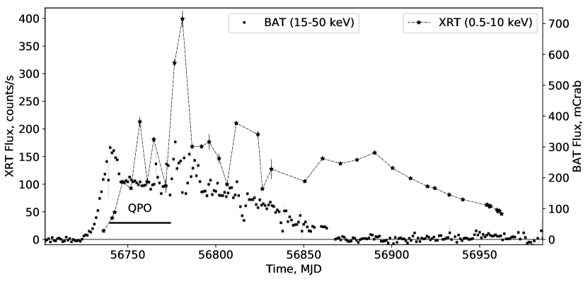
Рис. 1: Light curve of GRS 1739-278 during the 2014 outburst from Swift/XRT (designated by stars, the data were averaged over one observation) and Swift/BAT (designated by black squares, the data were averaged over one day) data. The horizontal line indicates the period of QPO observations in the variability power spectra for the source (observations 02-09).

Figure 1 shows the source’s light curve from Swift/XRT and Swift/BAT data in the 0.5-10 (the data points were averaged over one observation) and 15-50 keV (the data points were averaged over one day) energy bands, respectively. To convert the 15-50 keV flux to units corresponding to the flux from the Crab Nebula, we used the relation 1 Crab =0.22 counts s^-1 cm^-2. It can be seen from the figure that in the 15-50 keV energy band the flux from the source reached a maximum $\sim 0.3$ Crab $\sim 15$ days after the outburst onset, it then dropped by a factor of 1.5 in 5 days and was approximately at a constant level for $\sim 25$ days, after which it began to exhibit a peak-shaped variability that lasted for about 50 days and passed into the outburst decay phase. The emission from the source in this energy band ceased to be recorded $\sim 140$ days later.

In the 0.5-10 keV energy band the outburst reached its maximum ($\sim$1.1 Crab) with a delay relative to the maximum in the 15-50 keV energy band, 55 days after the onset, but the source exhibited a peak-shaped flux variability almost immediately from the outburst onset. On completion of this activity, 135 days after the outburst onset, the flux reached a constant level $\sim$150 counts s^-1 ($\sim$400 mCrab) and remained so for $\sim$30 days, after which it began to drop. The observations ceased on $\sim$240 day of the outburst, because the source fell into a region near the Sun inaccessible to observations. At this time the 0.5-10 keV flux was $\sim$50 counts s^-1 ($\sim$140 mCrab). In Fig. 2a the flux in the soft energy band (0.5- 10 keV) is plotted against the source’s hardness (the ratio of the 4-10 and 0.5-4 keV fluxes). It can be seen from the figure that the diagram has a shape that resembles the upper part of a typical "q"  diagram.

3.2 Spectral Analysis during the 2014 Outburst

When fitting the spectra, we used typical models describing the source’s spectrum: (1) in the low/hard state-a power law with a high-energy cutoff and low-energy absorption, phabs*cutoffpl (or in the case of fitting only the Swift/XRT data- a power law and low-energy absorption, phabs*powerlaw); (2) in the intermediate states-a power law with a high-energy cutoff, a multitemperature accretion disk, and low-energy absorption, phabs*(cutoffpl + diskbb) (or in the case of fitting only the Swift/XRT data-a power law, a multitemperature accretion disk, and low-energy absorption, phabs*(powerlaw + diskbb)); (3) in the high/soft state- a multitemperature accretion disk and low-energy absorption, phabs*diskbb, or the previous model, phabs*(powerlaw + diskbb). The quality of the available data does not allow us to apply the more complex spectral model including the reflection of Comptonized radiation from the accretion disk that was used in fitting the NuSTAR data (Miller et al. 2015; Mereminskiy et al. 2019).

The results of fitting the Swift/XRT spectra are presented in Table 1. The errors in the parameters are given for a 90% confidence interval. The table also provides the contribution of the unabsorbed power-law component to the total unabsorbed flux, the absorbed 0.8-10 keV flux, and the inner accretion disk radius estimated from the normalization in the diskbb model $N=(R_{in}/D_{10kpc})^{2}cosi$, where $R_{in}$ is the "apparent"  inner disk radius in km, $D_{10kpc}$ is the distance to the source in units of 10 kpc, and $i$ is the inclination to the plane of the sky. The distance to the source was taken to be 8.5 kpc.

When fitting the spectra obtained only from the Swift/XRT data, the available 0.8-10 keV energy band does not allow unambiguous constraints to be placed on the parameters of the power-law component in the case of using the multicomponent phabs*(powerlaw + diskbb) model. Therefore, when fitting the data at the initial outburst phases (from observation 03 to 09), we fixed the photon index at 1.5 and 1.8, which were derived when fitting the broadband spectra, at 2, and, in the subsequent observations, at 2 and 2.4, typical for the intermediate state (Remillard and McClintock 2006; Belloni and Motta 2016).

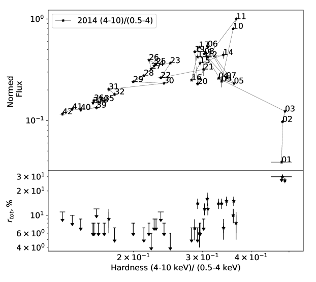
Рис. 2: Hardness-intensity and hardness-rms diagrams for the 2014 outburst. The hardness defined as the ratio of the count rates in the 4-10 and 0.5-4 keV energy bands is along the horizontal axis. (a) Swift/XRT photon count rate (in the 0.5-10 keV energy band) normalized to the maximum versus hardness. (b) Total fractional rms in the 0.5-10 keV energy band and the frequency range 0.01-50 Hz versus hardness. Each data point on the upper panel is labeled according to the observation number.

To fit the broadband spectra, we also used the phabs*highecut*simpl*diskbb model (the parameter $E_{c}$ in the highecut model was frozen at a minimum value of 0.0001 keV, which allowed the cutoffpl model to be imitated) that takes into account the physical cutoff of the power-law component at low energies in a simplified way. When estimating the errors in the parameters of the phabs*highecut*simpl*diskbb model, we fixed the absorption $N_{H}$ (and the parameter $f_{scat}$ for observation 03) at their values found. The results of fitting the broadband spectra are presented in Table 4. It can be seen from the table that this model gives a systematically larger inner accretion disk radius than does the model with the cutoffpl component, while the remaining parameters do not differ greatly.

It can be seen from Tables 1 and 4 that in observations 01-03 the model with a power law describes well the spectra, while in observation 03 the system’s spectrum can also be described by the power-law model with a multitemperature disk (the $\chi^{2}$ value is almost the same for the phabs*(powerlaw +diskbb) and phabs*powerlaw models). Beginning from the fourth observation, fitting the data by the model of a multitemperature disk with a power law is more preferable than that by the model only with a power law. Up to observation 23, fitting the data by a power law or a multitemperature disk with low-energy absorption gives a $\chi^{2}$ value systematically poorer than does the multicomponent model. In this case, the low-energy absorption, the temperature, and the inner radius of the accretion disk depend on the chosen photon index, i.e., the available data allow only the range of values (given in Table 1) in which the model parameters can lie to be specified.

Таблица 4: Parameters of the best-fit models $phabs*powerlaw$, $phabs*(diskbb+cutoffpl)$ and $phabs*highecut*simpl*diskbb$ with fixed $E_{c}=0.0001$ keV for the broadband energy spectra of GRS 1739-278.

$ID$	$C_{JEM-X}^{a}$	$C_{XRT}^{a}$	$N_{H}$, $10^{22}$cm${{}^{2}}^{b}$	$\Gamma^{c}$	$E_{cut}$, keV d	$f_{scat}^{e}$	$T_{in}$, keV f	$R_{in}cos^{-1/2}(i)$, km g	$f_{po}$, $\%^{h}$	Fluxj	$\chi^{2}/dof$
$01$	$0.51_{-0.08}^{+0.09}$	$1.24_{-0.34}^{+0.46}$	$1.9_{-0.42}^{+0.46}$	$1.45_{-0.21}^{+0.22}$	$95_{-29}^{+74}$		-	-	100	$1.2_{-0.5}^{+0.2}$	$1.76/17$
$03$	$0.74\pm 0.05$	$1.42_{-0.11}^{+0.12}$	$1.6\pm 0.04$	$1.2\pm 0.03$	$20.7_{-1.2}^{+1.4}$		-	-	100	$3.1\pm 0.2$	$1.22/506$
	$0.74\pm 0.05$	$1.42_{-0.12}^{+0.13}$	$1.84_{-0.15}^{+0.17}$	$1.21\pm 0.05$	$20.6_{-1.4}^{+1.5}$		$0.33_{-0.05}^{+0.09}$	$46_{-28}^{+48}$	93	$3.1_{-0.3}^{+0.2}$	$1.21/504$
	$0.73\pm 0.05$	$1.37_{-0.11}^{+0.12}$	$2.05$	$1.26_{-0.02}^{+0.03}$	$21.4_{-1.2}^{+1.3}$	0.68	$0.28\pm 0.01$	$211_{-22}^{+25}$		$3.2_{-0.3}^{+0.2}$	$1.22/506$
$05$	$0.81_{-0.07}^{+0.08}$	$1.8_{-0.16}^{+0.18}$	$1.83\pm 0.03$	$1.8\pm 0.03$	$35.9_{-3.9}^{+4.7}$		-	-	100	$3.9\pm 0.3$	$1.64/564$
	$0.84_{-0.07}^{+0.08}$	$2.19_{-0.21}^{+0.24}$	$2.04\pm 0.06$	$1.51_{-0.07}^{+0.06}$	$25.0_{-2.5}^{+2.9}$		$0.47_{-0.03}^{+0.04}$	$38.8_{-7.5}^{+10.0}$	80	$3.3_{-0.5}^{+0.2}$	$1.33/562$
	$0.84_{-0.07}^{+0.08}$	$2.21_{-0.21}^{+0.24}$	$1.93$	$1.5\pm 0.06$	$24.9_{-2.4}^{+2.9}$	$0.58\pm 0.01$	$0.47\pm 0.02$	$64.5_{-6.8}^{+8.2}$		$3.3_{-0.3}^{+0.2}$	$1.33/563$
$07$	$0.64\pm 0.03$	$1.54_{-0.09}^{+0.1}$	$2.15\pm 0.03$	$2.03\pm 0.03$	$38.5_{-2.8}^{+3.1}$		-	-	100	$5.3_{-0.3}^{+0.4}$	$1.61/524$
	$0.67_{-0.03}^{+0.04}$	$1.79_{-0.12}^{+0.13}$	$2.43_{-0.08}^{+0.09}$	$1.88\pm 0.05$	$32.2_{-2.4}^{+2.7}$		$0.38\pm 0.03$	$84.5_{-21.2}^{+29.5}$	81	$4.7_{-0.4}^{+0.3}$	$1.43/522$
	$0.67_{-0.03}^{+0.04}$	$1.8_{-0.12}^{+0.13}$	$2.34$	$1.87\pm 0.05$	$31.9_{-2.3}^{+2.6}$	$0.5\pm 0.02$	$0.38\pm 0.02$	$137.1_{-16.6}^{+20.6}$		$4.6_{-0.4}^{+0.2}$	$1.43/523$
$09$	$0.65\pm 0.05$	$1.22_{-0.10}^{+0.11}$	$1.95\pm 0.03$	$1.97\pm 0.03$	$37.0_{-3.7}^{+4.4}$		-	-	100	$5.3\pm 0.4$	$1.32/516$
	$0.71_{-0.05}^{+0.06}$	$1.54_{-0.14}^{+0.16}$	$2.08_{-0.06}^{+0.07}$	$1.67\pm 0.07$	$26.5_{-2.6}^{+3.0}$		$0.49\pm 0.04$	$40.4_{-8.1}^{+11.0}$	82	$4.3_{-0.6}^{+0.3}$	$1.11/514$
	$0.71_{-0.05}^{+0.06}$	$1.54_{-0.14}^{+0.15}$	$1.97$	$1.67_{-0.07}^{+0.06}$	$26.5_{-2.5}^{+2.9}$	$0.55\pm 0.02$	$0.48\pm 0.03$	$71.2_{-8.4}^{+10.3}$		$4.2_{-0.5}^{+0.3}$	$1.1/515$

a-cross-calibration constants for JEM-X and XRT relative to ISGRI, respectively; b-interstellar absorption; c-photon index; d- cutoff energy of the cutoffpl model; e-disk fraction subject to Comptonization (simpl); f-accretion disk temperature; g-inner disk radius for a distance to the system of 8.5 kpc; h-contribution of the power-law component to the total 0.8-10 keV flux; i-absorbed 0.8-10 keV flux of the broadband model, in units of $10^{-9}$ erg cm^-2 s^-1. The errors are given for a 90% confidence interval.

In observations 24-42 the data are well fitted by the model of a multitemperature disk with low-energy absorption. Although adding the power-law component when fitting some of the spectra formally reduces the $\chi^{2}$ value, the contribution of the powerlaw component is so small ($30\%$) that a change in the photon index within the range 2-2.4 has virtually no effect on the remaining model parameters.

3.3 Temporal Variability during the 2014 Outburst

To analyze the source’s variability, we constructed its power spectra in several energy bands: 0.5-10 (F), 0.5-3 (A), and 3-10 keV (B). QPOs were detected in the power spectra constructed for observations 02-09. As the best-fit model for the power spectra obtained in these observations we used a model consisting of two Lorentz profiles (one Lorentz profile described the broadband To analyze the source’s variability, we constructed its power spectra in several energy bands: 0.5-10 (F), 0.5-3 (A), and 3-10 keV (B). QPOs were detected in the power spectra constructed for observations 02-09. As the best-fit model for the power spectra obtained in these observations we used a model consisting of two Lorentz profiles (one Lorentz profile described the broadband

$$\begin{array}[]{l}P(f)=\frac{N_{qpo}}{\pi}\frac{\delta f_{qpo}/2}{(f-f_{qpo})^{2}+(\delta f_{qpo}/2)^{2}}+\\ \frac{N_{sub}}{\pi}\frac{\delta f_{sub}/2}{(f-f_{sub})^{2}+(\delta f_{sub}/2)^{2}}+P_{noise}\end{array}$$

where $f_{qpo}$ and $\delta f_{qpo}$ are the frequency and width of the Lorentzian responsible for the QPOs, $f_{sub}$ and $\delta f_{sub}$ are the frequency and width of the Lorentzian responsible for the broadband noise, $N_{qpo}$ and $N_{sub}$ are the normalizations of the QPO and broadband noise components, $P_{noise}$ is the constant responsible for the Poisson noise level. In the subsequent analysis we assumed that $f_{sub}$ = 0. This model describes well the power spectra of black hole candidates in the low/hard and low intermediate states (Belloni and Motta 2016).

To determine the parameters of the best-fit model, we used the maximum likelihood method (see Leahy et al. 1983; Vikhlinin et al. 1994). As the likelihood function we used the product of the probability density functions for a $\chi^{2}$ distribution with 2n degrees of freedom:

$$L=\prod{f_{\chi^{2}_{2n}}({{P_{i,src}2n}\over{P_{i,model}}})},$$ (1)

where $P_{i,src}$ is the measured rms power of the source in the i-th frequency bin, $P_{i,model}$ is the rms power of the source in the same bin obtained from the model, and n is the number of bins into which the light curve was partitioned.

Таблица 5: Best-fit parameters for the variability power spectra of GRS 1739-278.

$ID$	Banda	$\delta f_{qpo}$, Hz b	$f_{qpo}$, Hz c	$\delta f_{zl}$, Hz d	$Q=\frac{f_{qpo}}{\delta f_{qpo}}$ e	$rms_{qpo},\%$ f	$rms_{tot},\%$ f	$2\Delta L$ g( $log(p)$ h)
02	F	$0.03\pm 0.01$	$0.106\pm 0.004$	$0.33\pm 0.03$	$3.4\pm 1.3$	$13.9\pm 1.8$	$30.0\pm 1.0$	$39$($-7.8$)
	A	$0.04\pm 0.02$	$0.103\pm 0.005$	$0.32_{-0.05}^{+0.04}$	$8.0\pm 4.2$	$13.5_{-2.5}^{+2.3}$	$27.0\pm 1.0$	$28$($-5.4$)
	B	$0.03_{-0.02}^{+0.01}$	$0.113_{-0.012}^{+0.004}$	$0.31_{-0.04}^{+0.03}$	$4.2\pm 2.5$	$14.5_{-2.7}^{+2.4}$	$32.0\pm 1.0$	$27$($-5.2$)
03	F	$0.03\pm 0.01$	$0.377_{-0.003}^{+0.004}$	$0.62_{-0.04}^{+0.05}$	$11.7\pm 3.4$	$9.9_{-1.0}^{+0.9}$	$27.0\pm 1.0$	$81$($-16.7$)
	A	$0.03\pm 0.01$	$0.379\pm 0.005$	$0.57\pm 0.09$	$11.6\pm 5.1$	$8.7_{-1.3}^{+1.2}$	$23.0\pm 1.0$	$37$($-7.3$)
	B	$0.04\pm 0.01$	$0.377_{-0.004}^{+0.005}$	$0.61\pm 0.05$	$10.3\pm 3.6$	$11.2\pm 1.3$	$31.0\pm 1.0$	$58$( $-11.8$)
04	F	$0.29\pm 0.03$	$2.182\pm 0.012$	$1.59\pm 0.28$	$7.6\pm 0.9$	$10.3\pm 0.4$	$14.0\pm 1.0$	$338$($-72.2$)
	A	$0.32_{-0.11}^{+0.1}$	$2.208\pm 0.039$	$1.47_{-0.84}^{+0.64}$	$6.8\pm 2.3$	$7.2_{-0.9}^{+0.8}$	$10.0\pm 1.0$	$45$($-9.0$)
	B	$0.21\pm 0.03$	$2.19\pm 0.01$	$5.09_{-0.67}^{+0.64}$	$10.4\pm 1.5$	$13.5\pm 0.6$	$25.0\pm 1.0$	$295$($-62.9$)
05	F	$0.34\pm 0.04$	$1.69\pm 0.01$	$0.89_{-0.20}^{+0.19}$	$5.0\pm 0.6$	$12.6\pm 0.5$	$15.0\pm 0.0$	$262$($-55.8$)
	A	$0.31_{-0.13}^{+0.11}$	$1.73\pm 0.04$	$1.08_{-0.66}^{+0.44}$	$5.6\pm 2.3$	$7.7\pm 1.1$	$10.0\pm 1.0$	$31$($-6.1$)
	B	$0.24_{-0.03}^{+0.04}$	$1.7\pm 0.01$	$5.17_{-0.77}^{+0.83}$	$7.2\pm 1.1$	$15.5\pm 0.8$	$27.0\pm 1.0$	$235$( $-49.7$)
06	F	$0.4_{-0.17}^{+0.15}$	$5.07\pm 0.06$	$1.5_{-0.34}^{+0.32}$	$12.7\pm 5.3$	$6.7\pm 0.9$	$12.0\pm 1.0$	$32$($-6.3$)
	A	-	-	$0.75_{-0.52}^{+0.21}$	-	-	$6.0_{-2.0}^{+1.0}$	$0(-)$
	B	$0.24\pm 0.10$	$5.06\pm 0.03$	$2.18_{-0.48}^{+0.49}$	$21.1\pm 9.1$	$8.9\pm 1.2$	$19.0\pm 1.0$	$34$($-6.7$)
07	F	$0.48\pm 0.08$	$2.48\pm 0.03$	$0.93_{-0.19}^{+0.18}$	$5.2\pm 0.9$	$10.6\pm 0.6$	$15.0\pm 1.0$	$120$($-25.1$)
	A	$0.34_{-0.24}^{+0.20}$	$2.41\pm 0.09$	$0.99_{-0.58}^{+0.35}$	$7.1\pm 4.9$	$6.4_{-1.7}^{+1.5}$	$10.0\pm 1.0$	$13$($-2.3$)
	B	$0.49\pm 0.09$	$2.52\pm 0.03$	$1.12_{-0.22}^{+0.20}$	$5.1\pm 1.0$	$15.2_{-1.0}^{+0.9}$	$22.0\pm 1.0$	$90$($-18.7$)
08	F	$0.54_{-0.35}^{+0.33}$	$5.09\pm 0.14$	$1.08_{-0.38}^{+0.37}$	$9.4\pm 6.2$	$7.2\pm 1.6$	$12.0\pm 1.0$	$14$($-2.5$)
	A	-	-	$2.63_{-1.44}^{+1.04}$	-	-	$12.0\pm 2.0$	$0(-)$
	B	-	-	$9.55_{-3.78}^{+3.34}$	-	-	$21.0\pm 3.0$	$0(-)$
09	F	$0.31\pm 0.06$	$2.19\pm 0.02$	$0.28\pm 0.08$	$7.1\pm 1.5$	$11.7\pm 0.8$	$14.0\pm 1.0$	$91$($-18.9$)
	A	$0.39_{-0.23}^{+0.21}$	$2.25\pm 0.09$	$0.47_{-0.31}^{+0.10}$	$5.8\pm 3.5$	$7.4_{-1.5}^{+1.6}$	$10.0\pm 1.0$	$18$($-3.4$)
	B	$0.18\pm 0.05$	$2.15\pm 0.02$	$2.7_{-0.90}^{+0.92}$	$11.9\pm 3.1$	$15.0_{-1.3}^{+1.4}$	$25.0\pm 2.0$	$80$($-16.5$)

a-0.5-10 (F), 0.5-3 (A), and 3-10 keV (B) energy bands; b-width of the QPO peak; c-frequency of the QPO peak; d-width of the underlying component; e-QPO quality factor; f-QPO fractional rms and total fractional rms; g-statistic of the likelihood ratio test; h-logarithm of the probability that this difference of the likelihood functions is a random variable. The errors were determined for a 68% confidence interval (see the text).

To find the error in the parameters of the best-fit model, we used the Monte Carlo method. The data were randomly selected 1000 times around the best-fit model $P_{i,model}$ according to the law $P_{i}=\chi^{2}_{2n}(P_{i,model}/2n)$. The randomly selected data were also fitted by the model using the maximum likelihood method. The sought-for error in a parameter was found as a difference between the mean value and the lower (upper) limit on the parameter corresponding to the 16% (84%) quantile of the distribution.

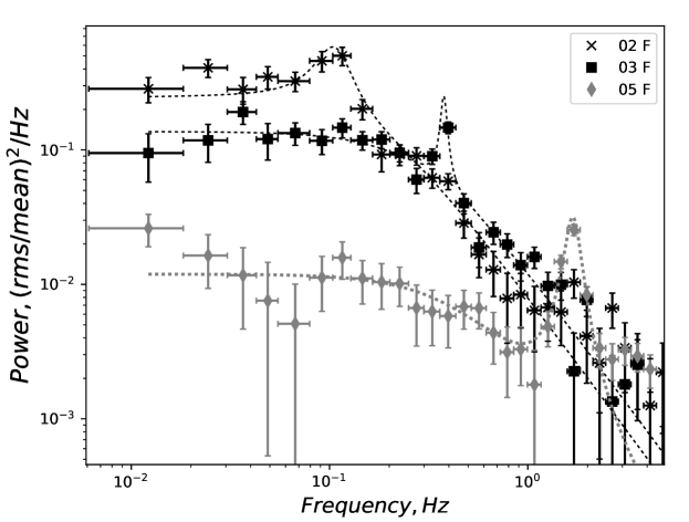
Рис. 3: Variability power spectra for the source in percentage normalization for observations 02 (black crosses), 03 (black squares), and 05 (gray diamonds) in the F (0.5-10 keV) band. The thin lines indicate the model fits to the spectra. The Poisson noise level was subtracted.

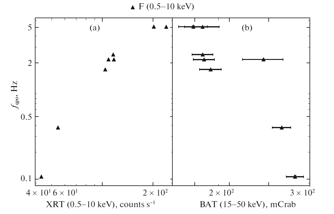
Рис. 4: (a) QPO frequency versus 0.8-10 keV flux. (b) QPO frequency versus 15-50 keV flux.

To determine the QPO significance, we calculated the doubled difference of logarithmic likelihood functions $2\log(L_{qpo}/L_{null})$, where $L_{qpo}$ and $L_{null}$ are the values of the likelihood function for the model with and without QPOs, respectively, and the probability that this difference is a random variable. The difference of the likelihood functions has a $\chi^{2}_{k}$ distribution (Cash 1979), where k is the difference of the numbers of free parameters in the models with and without QPOs, in our case, k = 3.

The results of fitting the power spectra with QPOs are presented in Table 5. No QPOs were recorded in observation 06 in the A band and in observation 08 in both and . For these power spectra we calculated an upper limit on the QPO fractional rms at 90$\%$ confidence by assuming the QPO frequency and quality factor in the A and B band to coincide with those in the F band. For observation 06 in the A band the upper limit is $r_{qpo}\leavevmode\nobreak\ <\leavevmode\nobreak\ 6\%$ ; in observation 08, $r_{qpo}\leavevmode\nobreak\ <\leavevmode\nobreak\ 10$ and 15$\%$ for the A and B bands, respectively. It can be seen from Table 5 that the QPO frequency does not depend on the energy band. Note that, as follows from the literature, the systems with black hole candidates show both no correlation between the QPO frequency and energy and direct and inverse proportionality (Yan et al. 2012; Li et al. 2013a, 2013b).

Figure 3 presents the power spectra with QPOs in the full energy band (0.5-10 keV) for several observations (02, 03, and 05). The QPO frequency is clearly seen to change from observation to observation.

To determine the type of QPOs, it is necessary to measure the parameters of both the QPO peak itself and the broadband noise. It follows from Fig. 3 and Table 5 that broadband noise whose total fractional rms is greater than 10$\%$ is present in the power spectra under study at low frequencies, which, as was said in the Introduction, is characteristic for type- C QPOs. We constructed the dependence of the QPO frequency on the flux in the soft (0.5-10 keV) and hard (15-50 keV) energy bands (Fig. 4). Since the contribution of the disk component in the 15- 50 keV energy band is minor, this may be considered as the dependence of the QPO frequency on the flux in the power-law component. It can be seen from the figure that the dependence of the QPO frequency on the flux in the soft and hard energy bands is direct and inverse, respectively; such a behavior is also characteristic for type-C QPOs (Motta et al. 2011). Stiele et al. (2011) showed that type-B QPOs are observed only at certain photon indices of the spectral component describing the Comptonized radiation. At the transition stage from the hard to soft state the photon index must be greater than or of the order of 2.2. In our case, it can be seen from Table 4 that the photon index is less than or of the order of 2, which again provides evidence for type-C QPOs.

For several systems, it was shown on the basis of Fourier spectroscopy that the corona makes a major contribution to the system’s variability (Churazov et al. 2001; Sobolewska and Zycki 2006), i.e., the fractional rms must decrease with decreasing contribution of the power-law component to the flux, which we observe. In observations 02 and 03, when the fractional rms in the A and B energy bands is determined by the power-law component, the total fractional rms in the soft energy band (A) is smaller than that in the hard (B) energy band by a factor of 1.2-1.3. At the same time, in observations 04-09, when the disk component is also present in the soft energy band, the fractional rms in the A band is smaller than that in the B band by a factor of 2-3.

For observations 10-42, when no QPOs were recorded, we determined the total fractional rms in the 0.5-10 keV energy band. For this purpose, we fitted the power spectra either by a power law with a constant or only by a constant by the maximum likelihood method. If we failed to extract the powerlaw component, then the source’s limiting white noise power was estimated. For this purpose, we searched for $P_{source}$ at which the measured power in the frequency range 0.01-50 Hz was the 10% quantile of the normal distribution $\mathcal{N}(P_{noise}+P_{source},(P_{noise}+P_{source})/Nn)$, where N is the number of frequency bins and $P_{source}$ is the measured Poisson noise level.

A diagram of the derived dependence of the total fractional rms on hardness (the ratio of the 4-10 and 0.5-4 keV fluxes) is shown in Fig. 2b. It follows from the figure that the total fractional rms of the source in the time of observations decreased from $\sim$30 to $\sim$8% or less.

3.4 Observed States during the 2014 Outburst

It follows from our spectral analysis (see Tables 1 and 4) that during observations 01-03 the photon index of the power-law component was $\sim 1.2-1.4$, while it follows from Table 5 that the total fractional rms during observations 02 and 03 was 30 and 27%, respectively. The values of these parameters suggest that the system was in the low/hard state in the period from observation 01 to 03.

From observation 04 to 09 the total fractional rms decreased to 12-15%, type-C QPOs were observed in the variability power spectrum, and the accretion disk contribution, along with the power-law component, is recorded in the source’s energy spectrum, which is typical for the hard intermediate state. The total fractional rms was $10\pm 2$ % during observation 10, $8\pm 3\%$ in observation 11, and 14-16% in observations 12 and 13, which also provides evidence for the hard intermediate state.

From observation 14 to 23 the source’s energy spectrum is still described by the model of an accretion disk with a power-law component, but the fractional rms of the source dropped below 10%. In many observations we managed to obtain only upper limits at a level <10%. Thus, it can be concluded that the system passed to the soft intermediate state between observations 13 and 14.

During observation 11 (when not only the total fractional rms, but also the contribution of the powerlaw component to the flux from the system decreased almost by a factor of 2 compared to the adjacent observations, see Table 1) the system may have passed to the soft intermediate state, but this cannot be asserted based on the available data. Despite the fact that fitting the data by the phabs*(diskbb +powerlaw) and phabs*diskbb models gives identical $\chi^{2}$ values, we think that the first model is most probable, because the source exhibits a significant flux (150 mCrab) in the 15-50 keV energy band.

From observation 24 to 42 the source’s energy spectra are well described by the model of a multitemperature disk with low-energy absorption, i.e., it can be argued that the system passed to the high/soft state. Although adding the power-law component when fitting some of the spectra formally reduces the $\chi^{2}$ value, nevertheless, first, the contribution of the power-law component is minor ($30\%$) and, second, a weak power-law can also be observed in the high/soft state (Belloni and Motta 2016). It is worth noting that the powerlaw model has no low-energy cutoff and the estimate of the contribution from the power-law component to the total flux is an upper limit, i.e., the fraction of the nonthermal component is actually smaller. Furthermore, it can be seen from Fig. 1 that after observation 23 the source is barely recorded in the 15-50 keV energy band, which also provides evidence for the transition to the high/soft state.

The source’s characteristic spectra corresponding to the low/hard, intermediate low/hard, and high/soft states (observations 01, 09, and 42, respectively) are presented in Fig. 5.

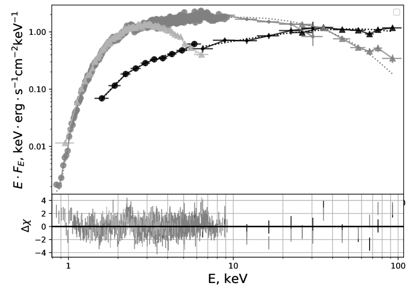
Рис. 5: Characteristic energy spectra of GRS 1739-278 and their best-fit-models during different spectral states: observation 01 (low/hard state)-black circles, dots, and triangles: the Swift/XRT, INTEGRAL/JEMX, and INTEGRAL/ISGRI data, respectively; observation 09 (intermediate state)-dark-gray circles, dots, and triangles: the Swift/XRT, INTEGRAL/JEMX, and INTEGRAL/ISGRI data, respectively; observation 42 (high/soft state)-light-gray triangles (Swift/XRT data). The thin dash-dotted lines indicate the best-fit models (see Tables 1 and 3). The lower panel shows the deviation of the data from the models.

Figure 6 shows the periods of time and the states in which the source was and presents the time dependences of the accretion disk temperature at the inner radius, the contribution of the power-law component to the total flux, and the total fractional rms. The accretion disk temperature at the inner radius and the contribution of the power-law component were taken from the model in which the photon index was fixed at 2.

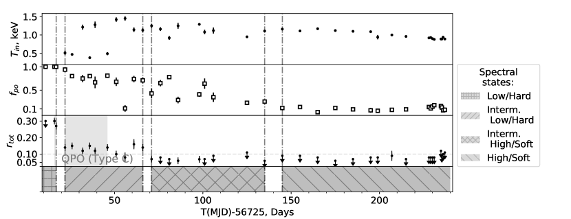
Рис. 6: (a) Accretion disk temperature at the inner radius versus time. (b) Contribution of the power-law component to the total flux versus time. (c) Total fractional rms versus time. The accretion disk temperature at the inner radius and the contribution of the power-law component are given for the model in which the photon index was fixed at 2. The periods of time when the source was in the low/hard, intermediate hard and soft, and high/soft states are also marked in the figure.

On the whole, our results on the transitions between states are consistent with those from Yan and Yu (2017) and Wang et al. (2018).

3.5 Mini-Outbursts of the System

We performed an analysis of the light curve for GRS 1739-278 over the entire period of observations since its discovery aimed at searching for undetected outbursts. From 1996 to mid-2011 the source was regularly observed by the ASM/RXTE all-sky monitor in the 1.2-12 keV energy band (Levine et al. 1996). According to these data, after the bright 1996 outburst the source exhibited no outburst activity and was not detected. Since 2005 the source has been observed almost continuously by the Swift/BAT telescope in the 15-50 keV energy band. From 2005 to 2014 no outbursts were detected on the light curve and the mean flux was $1.0\pm 0.4$ mCrab. After the end of the 2014 outburst the mean flux from the source rose to $9.7\pm 0.2$ mCrab.

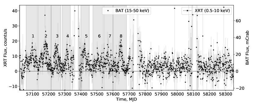
Рис. 7: Light curve of GRS 1739-278 for 2015-2016 from Swift/XRT (black stars, the data were averaged over one observation) and Swift/BAT (black squares, the data were averaged over one day) data. The shaded regions indicate the time intervals during which the outburst significance was determined (see the text and Fig. 8)

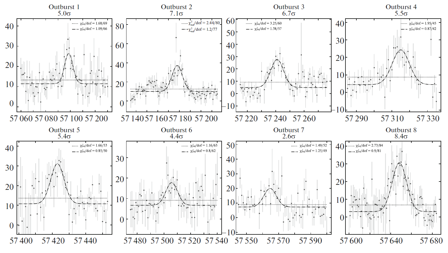
Рис. 8: Fitting the source’s outbursts detected from Swift/BAT data (15-50 keV) (see Fig. 7) by a constant (black dotted line) and a constant with the addition of a Gaussian profile (black dash-dotted line). The $\chi^{2}$ value is given for the fit by each model. The outburst detection significance is specified in the panel header.

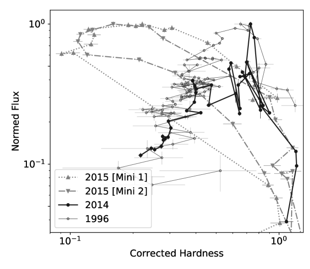
Рис. 9: Hardness-intensity diagram for the 1996 and 2014 outbursts as well as the first and second 2015 mini-outbursts (during which the system exhibited the transition from the low/hard to high/soft state), marked by the white circles, black circles, gray upper and lower triangles, respectively. The corrected hardness (see the text) is along the horizontal axis, the counts normalized to the maximum of each outburst is along the vertical axis: based on the ASM and XRT data in the 1.2-12 and 0.5-10 keV energy bands, respectively.

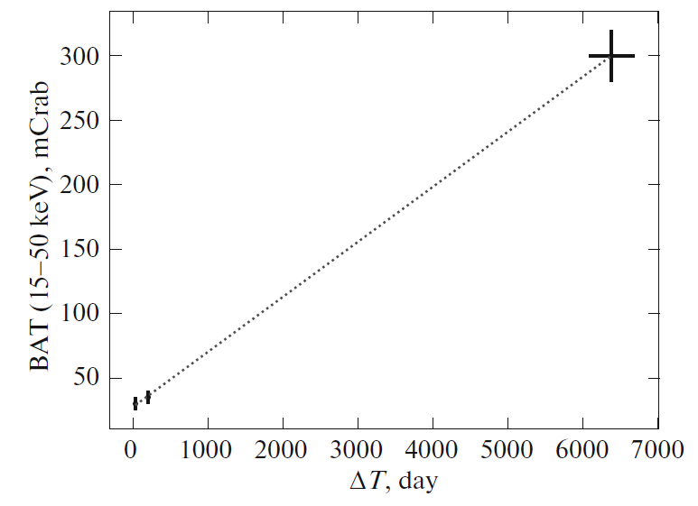
Рис. 10: BAT flux (in mCrab) at the peak of the outburst low/hard state versus time elapsed from the maximumin the low/hard state in the previous outburst. The dotted line indicates a linear best-fit model in the form 0.043 $mCrab/day$ $\Delta T$ + 27 mCrab.

A detailed analysis of the Swift/BAT light curve after the 2014 outburst showed that, apart from the mini-outbursts mentioned in the literature, the system exhibited several more similar events. To determine the statistical significance of the detected outbursts, we performed an analysis in which we partitioned the light curves into bins containing these outbursts (indicated by the gray rectangles in Fig. 7) and fitted the time dependence of the flux by two models: a constant and a constant with a Gaussian profile as the first approximation for the outburst profile. The outburst detection significance was defined as the probability of the difference of the $\chi^{2}$ values for both best-fit models (F-test). The results of our analysis are shown in Fig. 8; the outburst detection significance is given above each panel. It follows from the figure that the mini-outbursts mentioned in the literature had a significance of 7-8$\sigma$ (mini-outbursts 2, 3, and 8), while the detected four mini-outbursts have a significance of 4-5.5$\sigma$. Since outburst 7 has a low significance, 2.6$\sigma$, we did not include it in our final conclusions. After the failed 2016 outburst the system returned to a quiescent state with a mean flux of $5.0\pm 0.3$ mCrab.

3.6 Evolution of the Outbursts of the System in 1996, 2014, and 2015

Using the RXTE/ASM archival data, we constructed the hardness-intensity diagram for the 1996 outburst and compared it with that for the 2014 outburst and the 2015 mini-outbursts, when the system passed to the high/soft state. To make a proper comparison of the diagrams, it is necessary to take into account the difference in the energy bands and characteristics of the instruments. For this purpose, we calculated the hardness using the best-fit spectral models for several states. In the 1996 outburst we chose the KVANT/TTM observations on February 6-7, 1996, and the RXTE/PCA observations on March 31, 1996, and May 29, 1996 (see Borozdin et al. 1998). For the 2014 outburst we used observations 01, 11, and 32. The first observations for each outburst correspond to the time of the largest recorded hardness, the second observations refer to the time of the source’s maximum soft X-ray intensity, and the third observations refer to the high/soft state, when the power-law contribution to the total flux is minor. Using this sample of observations, we calculated the hardness for the 5-10 and 1.5-5 keV energy bands. The hardness ratios were found to be 1.29, 0.57, and 0.30, respectively, in the 1996 outburst and 1.29, 0.64, and 0.23 in the 2014 outburst. Having calculated the hardness from the light curves in the above reference observations, we found the ratios of the "true"  (based on the models) and observed (based on the light curves) hardnesses. The scatter of these ratios relative to the mean value is $12-15\%$; therefore, we used the mean value as a coefficient to convert the observed hardness-intensity diagram to the true one. The same coefficient was used For the 2014 outburst and the 2015 mini-outbursts. For the convenience of comparing the diagram shapes, we also normalized the flux to its maximum value. The derived diagrams are presented in Fig. 9. It can be seen from the figure that during the bright outbursts the curves have a similar shape, with the behavior of the source on the hardness-intensity diagram during the bright outbursts differing significantly from its behavior during the mini-outbursts. We estimated the luminosity at which a minimum hardness was reached during the outbursts by assuming the distance to the system to be 8.5 kpc: $L_{1.2-12\text{\,keV}}\sim 1.5\times 10^{37}$ erg s^-1 for the 1996 outburst, $L_{0.5-10\text{\,keV}}\sim 2\times 10^{37}$ erg s^-1 for the 2014 outburst, and$L_{0.5-10\text{\,keV}}\sim(5-6)\times 10^{36}$ erg s^-1 for the mini-outbursts.

Yu et al. (2007) and Wu et al. (2010) constructed the dependence of the peak flux in the 20-160 keV energy band during the low/hard state on the time between the current and previous peak fluxes in the low/hard state for GX 339-4 (a low-mass binary system with a black hole candidate) and attempted to fit this dependence by a linear law. We constructed the same dependence of the peak flux in the 15-50 keV energy band in the low/hard state on the time to the previous peak in the low/hard state for GRS 1739-278 by taking into account the bright 1996 and 2014 outbursts and the 2015 mini-outbursts (Fig. 10). The time of the transition to the hard state at the end of the 2014 outburst was taken from Wang et al. (2018). The linear dependence that best fits the data for GRS 1739-278 looks as follows: $F_{hard}(\Delta T)=(0.043\pm 0.003)\frac{\text{mCrab}}{\text{day}}\Delta T+(27\pm 2)\text{mCrab}$.

4 CONCLUSIONS

In this paper we performed a joint study of the spectral and temporal evolution of GRS 1739-278 during the 2014 outburst and made a comparative analysis of the system’s behavior during the remaining outbursts mentioned in the literature and in the periods between them. Our results can be briefly summarized as follows.

• We showed that during the 2014 outburst the system passed to the hard intermediate state 22 days after the outburst onset, to the soft intermediate state 66 days later (possibly exhibiting this state on day 55 and returning to the hard intermediate state no later than 4 days after), and to the high/soft state 145 days later.

• QPOs in the frequency range 0.1-5 Hz were detected during the outburst of GRS 1739-278 in 2014. All QPOs are type-C ones. No energy dependence of the QPO frequency was found.

• We showed that after the 2014 outburst the system passed to the regime of mini-outburst activity and, apart from the three mini-outbursts mentioned in the literature (Yu and Yan 2017; Mereminskiy et al. 2017), we detected four more mini-outbursts with a comparable ($\sim$20 mCrab) flux in the hard energy band (15-50 keV).

• We showed that the hardness-intensity diagram for the 2015 mini-outbursts, during which the system exhibited the transition to the high/soft state, differs from that for the bright 1996 and 2014 outbursts: the minimum hardness during the mini-outbursts was reached at fluxes of at least $60-80\%$ of the peak one, while in the bright outbursts the minimum hardness was reached at fluxes of $\sim 10\%$ of the peak one. The 0.5-10 keV luminosity of the source corresponding to these times differed approximately by a factor of 3: $L_{0.5-10\text{\, keV}}\sim 2\times 10^{37}$ erg s^-1 for the bright outburst and $L_{0.5-10\text{\,keV}}\sim(5-6)\times 10^{36}$ erg s^-1 for the mini-outbursts.

• We constructed the dependence of the peak flux in the hard energy band during the low/hard state on the time interval between outbursts. This dependence can be fitted by a linear law, which may point to the dependence of the system’s peak flux in the low/hard state on the mass of the accretion disk being accumulated.

5 ACKNOWLEDGMENTS

This work was financially supported by RSF grant no. 14-12-01287. We used the data provided by the UK Swift Science Data Center at the University of Leicester and the INTEGRAL Science Data Centers at the University of Geneva and the Space Research Institute of the Russian Academy of Sciences.

6 REFERENCES

• 1. K. A. Arnaud, Astron. Data Anal. Software Syst. V 101, 17 (1996).

• 2. T. M. Belloni, Lect. Notes Phys. 794, 53 (2010).

• 3. T. M. Belloni and S. E. Motta, Astrophys. Space Sci. Lib. 440, 61 (2016).

• 4. K. N. Borozdin and S. P. Trudolyubov, Astrophys. J. 533, L131 (2000).

• 5. K. Borozdin, N. Alexandrovich, R. Sunyaev, et al., IAU Circ. 6350 (1996).

• 6. K.N. Borozdin, M. G. Revnivtsev, S. P. Trudolyubov, et al., Astron. Lett. 24, 435 (1998).

• 7. D. N. Burrows, J. E. Hill, J. A. Nousek, et al., Space Sci. Rev. 120, 165 (2005).

• 8. F. Capitanio, T. Belloni, M. del Santo, et al., Mon. Not. R. Astron. Soc. 398, 1194 (2009).

• 9. W. Cash, Astrophys. J. 228, 939 (1979).

• 10. P. Durouchoux, I. A. Smith, K. Hurley et al., IAU Circ. 6383, 1 (1996).

• 11. P. A. Evans, A. P. Beardmore, K. L. Page, et al., Astron. Astrophys. 469, 379 (2007).

• 12. C. Ferrigno, E. Bozzo, M. del Santo, et al., Astron. Astrophys. 537, L7 (2012).

• 13. E. Filippova, E. Bozzo, and C. Ferrigno, Astron. Astrophys. 563, A124 (2014a).

• 14. E. Filippova, E. Kuulkers, N.M. Skadt, et al., Astron. Telegram 5991, 1 (2014b).

• 15. F. Furst, M. A. Nowak, J. A. Tomsick, et al., Astrophys. J. 808, 122 (2015).

• 16. M. R. Gilfanov, Lect. Notes Phys. 794, 17 (2010).

• 17. S. Grebenev, R. Sunyaev,M. Pavlinsky, et al., Astron. Astrophys. Suppl. Ser. 97, 281 (1993).

• 18. S. Grebenev, R. Sunyaev, and M. Pavlinsky, Adv. Space Res. 19, 15 (1997).

• 19. J. Homan, R. Wijnands,M. van der Klis, et al., Astrophys. J. 132, 377 (2001).

• 20. A. Ingram, C. Done, and P. C. Fragile,Mon. Not. R. Astron. Soc. 397, L101 (2009).

• 21. M. van der Klis, in Timing Neutron Stars, Ed. by H. Ogelman and E. P. J. van den Heuvel, NATO ASI Ser. C 262, 27 (1988).

• 22. H. A. Krimm, S. T. Holland, R. H. D. Corbet, et al., Astrophys. J. 209, 14 (2013).

• 23. H. A. Krimm, S. D. Barthelmy, W. Baumgartner, et al., Astron. Telegram 5986, 1 (2014).

• 24. D. A. Leahy,W. Darbro,R. F. Elsner, et al., Astrophys. J. 266, 160 (1983).

• 25. A.M. Levine, H. Bradt, W. Cui, et al., Astrophys. J. 469, L33 (1996).

• 26. Z. B. Li, J. L. Qu, L.M. Song, et al., Mon. Not. R. Astron. Soc. 428, 1704 (2013a).

• 27. Z. B. Li, S. Zhang, J. L. Qu, et al., Mon. Not. R. Astron. Soc. 433, 412 (2013b).

• 28. I. Mereminskiy, R. Krivonos, S. Grebenev, et al., Astron. Telegram 9517, 1 (2016).

• 29. I. A. Mereminskiy, E. V. Filippova, R. A. Krivonos, S. A. Grebenev, R. A. Burenin, and R. A. Sunyaev, Astron. Lett. 43, 167 (2017).

• 30. I. A. Mereminskiy, A. N. Semena, S.D. Bykov, et al., Mon. Not. R. Astron. Soc. 482, 1392 (2019).

• 31. J. M. Miller, J. A. Tomsick, M. Bachetti, et al., Astrophys. J. 799, L6 (2015).

• 32. S.Motta, T.Munoz-Darias, and T.Belloni,Mon.Not. R. Astron. Soc. 408, 1796 (2010).

• 33. S. Motta, T. Munoz-Darias, P. Casella, et al., Mon. Not. R. Astron. Soc. 418, 2292 (2011).

• 34. J. Paul, L. Bouchet, E. Churazov, et al., IAU Circ. 6348, 1 (1996).

• 35. R. A. Remillard and J. E. McClintock, Ann. Rev. Astron. Astrophys. 44, 49 (2006).

• 36. J. Rodriguez, S. Corbel, E. Kalemci, et al., Astrophys. J. 612, 1018 (2004).

• 37. M. del Santo, T.M. Belloni, J. A. Tomsicket al.,Mon. Not. R. Astron. Soc. 456, 3585 (2016).

• 38. D. M. Smith, W. A. Heindl, C. B. Markwardt, et al., Astrophys. J. 554, L41 (2001).

• 39. M. A. Sobolewska and P. T. Zycki, Mon. Not. R. Astron. Soc. 370, 405 (2006).

• 40. J. F. Steiner, R. Narayan, J. E. McClintock, et al., Publ. Astron. Soc. Pacif. 121, 1279 (2009).

• 41. H. Stiele, S. Motta, T. Munoz-Darias, et al., Mon. Not. R. Astron. Soc. 418, 1746 (2011).

• 42. Y. Tanaka and N. Shibazaki, Ann. Rev. Astron. Astrophys. 34, 607 (1996).

• 43. M. Vargas, A. Goldwurm, J. Paul, et al., Astron. Astrophys. 313, 828 (1996).

• 44. A. Vikhlinin, E. Churazov, M. Gilfanov, et al., Astrophys. J. 424, 395 (1994).

• 45. R. Walter, R. Rohlfs, M. T. Meharga, et al., in Proceedings of the 8th Integral Workshop on The Restless Gamma-ray Universe INTEGRAL 2010, PoS(INTEGRAL2010)162.

• 46. S.Wang, N. Kawai,M. Shidatsu, et al., Publ. Astron. Soc. Jpn. 70, 67 (2018).

• 47. Y. X.Wu,W.Yu, Z. Yan, et al., Astron. Astrophys. 512, A32 (2010).

• 48. S. P. Yan, J. L. Qu, G. Q. Ding, et al., Astron. Astrophys. Suppl. Ser. 337, 137 (2012).

• 49. Z. Yan and W. Yu, Mon. Not. R. Astron. Soc. 470, 4298 (2017).

• 50. W. Yu and Z. Yan, Astrophys. J. 701, 1940 (2009).

• 51. W. Yu, M. van der Klis, and R. Fender, Astrophys. J. 611, L121 (2004).

• 52. W.Yu, F. K.Lamb,R.Fender, et al., Astrophys. J. 663, 1309 (2007).

• 53. A. A. Zdziarski,M.Gierlinski, J.Mikolajewska, et al., Mon. Not. R. Astron. Soc. 351, 791 (2004).