MS-OPT-19-01028.R1

Chen and Mišić

Decision Forest: A Nonparametric Approach to Modeling Irrational Choice

Decision Forest: A Nonparametric Approach to Modeling Irrational Choice

Yi-Chun Chen UCLA Anderson School of Management, University of California, Los Angeles, California 90095, United States, yi-chun.chen.phd@anderson.ucla.edu Velibor V. Mišić UCLA Anderson School of Management, University of California, Los Angeles, California 90095, United States, velibor.misic@anderson.ucla.edu

Customer behavior is often assumed to follow weak rationality, which implies that adding a product to an assortment will not increase the choice probability of another product in that assortment. However, an increasing amount of research has revealed that customers are not necessarily rational when making decisions. In this paper, we propose a new nonparametric choice model that relaxes this assumption and can model a wider range of customer behavior, such as decoy effects between products. In this model, each customer type is associated with a binary decision tree, which represents a decision process for making a purchase based on checking for the existence of specific products in the assortment. Together with a probability distribution over customer types, we show that the resulting model – a decision forest – is able to represent any customer choice model, including models that are inconsistent with weak rationality. We theoretically characterize the depth of the forest needed to fit a data set of historical assortments and prove that with high probability, a forest whose depth scales logarithmically in the number of assortments is sufficient to fit most data sets. We also propose two practical algorithms – one based on column generation and one based on random sampling – for estimating such models from data. Using synthetic data and real transaction data exhibiting non-rational behavior, we show that the model outperforms both rational and non-rational benchmark models in out-of-sample predictive ability.

nonparametric choice modeling; decision trees; non-rational behavior; linear optimization First version: April 22, 2019. Second version: May 18, 2020. This version: July 25, 2021. Forthcoming in Management Science.

1 Introduction

A common problem in business is to decide which products to offer to customers by using historical sales data. The problem can be generally stated as follows: a firm offers a set of products (an assortment) to a group of customers. Each customer makes a decision to either purchase one of the products or not purchase any of the products. The goal of the firm is to decide which products to offer, so as to maximize the expected revenue when customers exercise their preferences.

In order to make such decisions, it is critical to have access to a model for predicting customer choices. Customer choice models have been used to model and predict the substitution behavior of customers when they are offered different assortments of products. In general, a choice model can be thought of as a conditional probability distribution over all purchase options given an assortment that is offered. A rich literature spanning marketing, psychology, economics, and operations management has contributed to the understanding of choice models.

A widely-used assumption is that customers are rational, i.e., choice models are assumed to follow rational choice theory and are based on the random utility maximization (RUM) principle. The RUM principle requires that each product is endowed with a stochastic utility. When a customer encounters the assortment and needs to make a purchase decision, all utilities are realized and the customer will choose the product from the assortment with the highest realized utility. A consequence of the RUM principle is that whenever we add a product to an assortment, the choice probability of each incumbent product either stays the same or decreases. This property is known as regularity or weak rationality.

However, customers are not always rational. There is an increasing body of experimental evidence, arising in the fields of marketing, economics, and psychology, which suggests that the aggregate choice behavior of individuals is not always consistent with the RUM principle and often violates the weak rationality property. A well-known example is the experiment involving subscriptions to The Economist magazine from Ariely (2008), which is re-created in Table 1. One hundred MIT students were asked to make decisions given two different assortments of subscription options. In the first assortment in Table 1, two subscription options are given: “Internet-Only” ($59.00) and “Print-&-Internet” ($125.00). The first option is chosen by the majority of the students (68 out of 100). In the second assortment, the students are given one more option: “Print-Only” ($125.00). For this second assortment, due to the obvious advantage in “Print-&-Internet” over “Print-Only”, no one chose the latter option. But with the addition of the the “Print-Only” option, the number of subscribers of the “Print-&-Internet” option actually increased from $32$ to $84$, thus demonstrating a violation of the weak rationality property. Here, the option “Print-Only” serves as a decoy or an anchor: its presence can influence an individual’s preference over the two other options “Internet-Only” and “Print-&-Internet”. While this example comes from a classroom experiment, there has been an extensive peer-reviewed research literature on this phenomenon, known as the decoy or attraction effect, since the seminal work of Huber et al. (1982).

Table 1: Behavioral experiment involving subscriptions to The Economist; reproduced from Ariely (2008)

Option	Price	Num. of Subscribers
Internet-Only	$59.00	68
Print-&-Internet	$125.00	32
Option	Price	Num. of Subscribers
Internet-Only	$59.00	16
Print-Only	$125.00	0
Print-&-Internet	$125.00	84

The example that we have described above is important for two reasons. First, even for this very simple example, no choice model based on RUM can perfectly capture the subscribers’ observed behaviors; as such, choice predictions based on RUM models will be inherently biased if customers do not behave according to a RUM model. Second, the presence of irrationality in customer choice behavior can have significant operational implications on which products should be offered. As a concrete example, observe that in Table 1, assuming that customers have no outside option, the expected per-customer revenue arising from the first assortment is $80.12, whereas the expected per-customer revenue of the second assortment is $114.44 – an increase of more than 40%! Indeed, outside of experimental settings (as in the above example), deviations from rational behavior have been observed – and exploited – in business practice. For example, when Williams-Sonoma observed low sales of a bread bakery machine priced at $275, it introduced a larger and more expensive version priced at $429; few customers bought the new model, but sales of the original model almost doubled (Poundstone 2010).

In this paper, we propose a new type of choice model, called the decision forest model, that is flexible enough to model non-rational choice behavior, i.e., choice behavior that is inconsistent with the RUM principle. In this choice model, one assumes that the customer population can be described as a finite collection of customer types, where each customer type is associated with a binary decision tree, together with a probability distribution over those types. Each decision tree defines a sequence of queries that the customer follows in order to reach a purchase decision, where each query involves checking whether a particular product is contained in the assortment or not.

We make the following specific contributions:

1. Model: We propose a new model for customer choice based on representing the customer population as a probability distribution over decision trees. We provide several examples of how well-known behavioral anomalies, such as the decoy effect and the preference cycle, can be represented by this model. We also prove a key theoretical result: any choice model, whether it obeys the RUM property or not, can be represented as a probability distribution over binary decision trees. As a result, our model can be regarded as a nonparametric model for general choice behavior.

2. Model complexity guarantees: We consider the problem of how to estimate our forest model from data and establish two guarantees on the complexity of the trees required to learn the model. Our first result states that for any data set of $M$ historical assortments for $N$ products there exists a decision forest model consisting of $M(N+1)+1$ trees, each of depth at most $\min\{M+1,N+1\}$ and with at most $2M$ leaves, that perfectly fits the data. Our second result states that with very high probability over the sample of $M$ historical assortments, forests consisting of trees of depth scaling logarithmically with the number of assortments $M$ are sufficient to perfectly fit the data. Thus, when data is limited, we can use less complex (simpler) models to fit the data.

3. Estimation methods: We formulate the problem of estimating the decision forest model from data as an optimization problem and propose two solution methods. The first method, based on column generation, involves sequentially adding new trees to a growing collection. While this approach guarantees optimality when the column generation subproblem is solved exactly as an integer program, it is not computationally scalable. We thus propose a top-down learning algorithm for heuristically solving the subproblem, leading to a heuristic column generation approach. The second method, called randomized tree sampling, is based on randomly sampling a large number of trees and then finding the corresponding probability distribution over these trees by solving an optimization problem. This method removes the computational effort needed to search for decision trees by generating them through a simple and efficient randomization scheme. We provide a theoretical result to justify the usage of this method showing that the training error of the obtained model is bounded by the error of a model defined relative to the sampling distribution plus a term that decays with rate $1/\sqrt{K}$, where $K$ is the number of sampled trees.

4. Practical performance: We evaluate the performance of our proposed model using real sales data from the IRI Academic Data Set (Bronnenberg et al. 2008) and compare to other methods in the literature. We show that decision forest models lead to a significant improvement in out-of-sample prediction, as measured by Kullback-Leibler divergence, over the multinomial logit (MNL) model, the latent-class MNL model, the ranking-based model, and the HALO-MNL model (Maragheh et al. 2018) across a large range of product categories. We also demonstrate how the decision forest model can be used to extract insights about substitution and complementarity effects and identify interesting customer behaviors within a specific product category.

The rest of this paper is organized as follows. In Section 2, we review the relevant literature in rational and non-rational choice modeling. In Section 3, we present our decision forest model and theoretically characterize its expressive power. In Section 4, we present our theoretical results on model complexity. In Section 5, we present our two estimation methods. In Section 6, we numerically show the effectiveness of our approach on real-world data. In Section 7, we conclude. All proofs are provided in the electronic companion, along with additional numerical experiments based on real and synthetic data.

2 Literature Review

In this section, we review the relevant literature. We first review prior work in rational choice modeling (Section 2.1), followed by prior research in non-rational choice modeling (Section 2.2). As a key contribution of this paper is the universality property of the decision forest model (see Theorem 3.2 in Section 3.6), in Section 2.3, we review two classes of choice models that also share this property and compare them with our model. Finally, we relate our proposed model to other research areas in Section 2.4.

2.1 Rational Choice Modeling

Numerous discrete choice models have been proposed based on the RUM principle, such as the multinomial logit (MNL), latent-class MNL (LC-MNL), and nested logit (NL) model; we refer the reader to Ben-Akiva and Lerman (1985) and Train (2009) for more details.

There has been a significant effort to develop “universal” choice models. A well-known universality result in choice modeling comes from the paper of McFadden and Train (2000), which showed that any RUM choice model can be approximated to an arbitrary precision by a mixture of MNL models. Outside of logit models, earlier research proposed the ranking-based model (also known as the stochastic preference model), in which one represents a choice model as a probability distribution over rankings; Block and Marschak (1959) showed that the class of RUM choice models is equivalent to the class of ranking-based models. Later, the seminal paper of Farias et al. (2013) developed a data-driven approach for making revenue predictions via the ranking-based model; specifically, the method involves computing the worst-case revenue of a given assortment over all ranking-based models that are consistent with the available choice data. Subsequent research on ranking-based models has studied other estimation approaches (van Ryzin and Vulcano 2014, Mišić 2016, Jagabathula and Rusmevichientong 2016, 2019), as well as methods for obtaining optimal or near-optimal assortments (Aouad et al. 2015, 2018a, Feldman et al. 2018, Bertsimas and Mišić 2019). Another model is the Markov chain model of customer choice (Blanchet et al. 2016). By modeling substitution behavior between products as transitions between states in the Markov chain, the model provides a good approximation to any choice model based on the RUM principle. Since the original paper of Blanchet et al. (2016), later research has considered other methods of estimating such models from limited data (Şimşek and Topaloglu 2018) as well as methods for solving core revenue management problems under such models (Feldman and Topaloglu 2017, Désir et al. 2015a, b). In a different direction, the papers of Natarajan et al. (2009) and Mishra et al. (2014) proposed the marginal distribution model, which is the choice model obtained by finding the joint distribution of errors in the random utility model that is consistent with given marginal error distributions and maximizes the customer’s expected utility.

As discussed before, there exist many experimental and empirical examples of choice behavior that deviates from RUM, and thus cannot be modeled using the ranking-based model. Our model, on the other hand, is general enough to represent models that cannot be represented using RUM. Our model can be regarded as a natural extension of the nonparametric model of Farias et al. (2013) to the realm of non-rational choice models.

2.2 Non-rational Choice Modeling

The study of non-rational choice has its roots in the seminal work of Kahneman and Tversky (1979), which demonstrated how expected utility theory fails to explain certain choice phenomena, and proposed prospect theory as an alternative model. Since this paper, significant research effort has been devoted to the study of non-rational decision making. Within this body of research, our work relates to the significant empirical and theoretical work in behavioral economics on context-dependent choice (Tversky and Simonson 1993), which includes important context effects such as the compromise effect (Simonson 1989), the attraction effect (Huber et al. 1982), and the similarity effect (Tversky 1972).

Recently, new choice models have been proposed for modeling behavior outside of the RUM class. Within behavioral economics, examples include the generalized Luce model (Echenique and Saito 2015) and the perception-adjusted Luce model (PALM) (Echenique et al. 2018). The focus of these papers is descriptive, in that they develop axiomatic theories for new models. In contrast, the focus of our paper is prescriptive, as we develop optimization-based methods for estimating our decision forest models from limited data.

Within operations management, examples of new choice models include the general attraction model (GAM) (Gallego et al. 2014), the HALO-MNL model (Maragheh et al. 2018) and the generalized stochastic preference (GSP) model (Berbeglia 2018). The main difference between our model and these prior models is in expressive power. As we will show in Section 3.6, our choice model is universal and is able to represent any discrete choice model that may or may not be in the RUM class; in contrast, for each of the generalized Luce model, PALM, GAM, HALO-MNL model and GSP model, there either exist choice models that do not obey the RUM principle and cannot be represented by the model, or the representational power of the model is unknown.

Lastly, the recent paper of Jagabathula and Rusmevichientong (2019) introduced the concept of loss of rationality. The loss of rationality is defined as the lowest possible information loss attained by fitting an RUM model to a given choice dataset; in other words, it is the lack of fit between the given data and the entire RUM class. By computing this lack of fit, one can determine whether it is necessary to consider models outside of the RUM class. The focus of our paper is different, in that we propose a specific answer to the question of how one should model customer behavior that may be irrational, and as such is complementary to that of Jagabathula and Rusmevichientong (2019).

2.3 Previous Universality Results

Within the economics literature, there are two classes of non-rational models that have the same expressive power as the decision forest model. We review these two classes of models in detail, followed by our contribution to this “universality” paradigm.

The first is the class of game tree models and randomized game tree models. The game tree model was proposed by Xu and Zhou (2007) as a model for how an option is deterministically chosen from a given choice set. In a game tree model, the tree encodes a hierarchy where each leaf corresponds to a product, and each non-leaf node correspond to a decision maker that is endowed with a ranking over the product universe. To make a decision, one starts at the non-leaf nodes whose children are leaves, and the decision maker at each such non-leaf node chooses its most preferred product according to its ranking. The parent nodes of those non-leaf nodes then choose from the products chosen by their children. This process repeats until reaching the decision maker at the root of the tree who makes the final decision. The model can thus be thought of as a representation of how an organization, through several rounds of decision making, reaches a decision. This type of model bears a superficial similarity to ours in that both models involve trees. However, the details differ significantly: in our trees, the decision process starts at the root (rather than the leaves) and involves checking for the existence/non-existence of a product in the assortment, until reaching a leaf. In addition, the trees that we describe are always binary, whereas game trees can in general be non-binary trees. Since the paper of Xu and Zhou (2007), other research has extended this type of model in different ways. For example, Horan (2011) considers game trees where all of the decision makers follow the same ranking. In the subsequent literature, the paper of Li and Tang (2017) considers the randomized game tree model, where one assumes a probability distribution over the tuple of rankings for the non-leaf nodes; that paper shows that this model can represent any discrete choice model, which is similar to our universality result (Theorem 3.2 in Section 3.6).

The second type of model that has the universality property is the pro-con model in the working paper of Dogan and Yildiz (2018). In this choice model, one considers two sets of rankings: “pro” rankings and “con” rankings. Then, over the union of the pro and con rankings, one posits a signed probability distribution, where the pro rankings receive positive probabilities, and the con rankings receive negative probabilities. The choice probability of a product given an assortment is the sum of the (positive) probabilities for the pro rankings for which that product is highest ranked, plus the sum of the (negative) probabilities for the con rankings for which that product is lowest ranked. The model aims to represent the idea of a decision maker who makes decisions by listing the pros and cons of an option, adding up the pros and subtracting the cons. The main result of Dogan and Yildiz (2018) is the result that every choice model can be represented as a pro-con model, which is again similar to our universality result (Theorem 3.2 in Section 3.6). While that paper develops a similar universality result, the proof requires a very careful induction argument, results from number theory and results from network flow optimization; in contrast, the proof of our universality result is simpler, requiring one to only define a specific and intuitively-chosen family of trees and to re-arrange sums.

While these two classes of models also have the universality result, to date, all research on the game tree models and the pro-con model has been theoretical and descriptive in nature, and has focused on categorizing and relating these models to existing models. These papers do not include methodological contributions: specifically, there has not been any research that answers the question of how to efficiently estimate these models from data, and that empirically validates these models on real data. In contrast, in our paper, we show that our proposed model can be estimated from data in two tractable ways (Section 5), and its performance can be validated using real transaction data (Section 6). Stated more concisely, the main contribution of our paper is a universal choice model that is practical and ready to be used by practitioners for real-world applications.

2.4 Other areas

Lastly, our model is also related to the rich literature on tree models in machine learning. Many machine learning methods construct binary tree models that can be used for classification or regression, such as ID3 (Quinlan 1986), C4.5 (Quinlan 1993) and classification and regression trees (CART; Breiman et al. 1984). In addition, there are also many predictive models that consist of ensembles or forests of trees, such as random forests (Breiman 2001) and boosted trees (Freund and Schapire 1996). The main difference between our work and prior work in machine learning is in the use of forests for discrete choice modeling, that is, using a forest to probabilistically model how customers choose from an assortment. To the best of our knowledge, the use of tree ensemble models for discrete choice modeling has not been proposed before.

We do note that some work in operations management has considered the use of tree ensemble models for demand modeling. Two examples of such papers are Ferreira et al. (2015) and Mišić (2020), which use random forests to model aggregate demand or profit as a function of product prices. These papers, however, do not model substitution effects as a function of the product assortment.

3 Decision Forest Customer Choice Model

In this section, we present our decision forest choice model. We begin in Section 3.2 by introducing binary decision trees and defining how customers make purchases according to such decision trees. We then define our choice model in Section 3.3, and compare it to the ranking-based model in Section 3.4. We describe a couple of well-known examples of behavioral anomalies that can be represented by our model in Section 3.5. Finally, we establish our first key theoretical result, namely that decision forest models can represent any customer choice model, in Section 3.6.

3.1 Choice Modeling Background

Consider a universe of $N$ products, denoted by the set $\mathcal{N}\equiv\{1,2,\ldots,N\}$. The full set of purchase options is denoted by $\mathcal{N}^{+}\equiv\{0,1,2,\ldots,N\}$, where $0$ corresponds to an outside or “no-purchase” option. An assortment $S$ is a subset of $\mathcal{N}$. When offered the assortment $S$, the customer may choose to purchase one of the products in $S$, or choose the no-purchase option 0.

The behavior of the customer population is represented through a discrete choice model. A discrete choice model is defined as a conditional probability distribution $\mathbf{P}(\cdot\mid\cdot):\mathcal{N}^{+}\times 2^{\mathcal{N}}\rightarrow[0,1]$ that gives the probability of an option in $\mathcal{N}^{+}$ being purchased when the customer is offered a particular set of products; that is, $\mathbf{P}(o\mid S)$ is the probability of the customer choosing the option $o\in S\cup\{0\}$, when offered the assortment $S\subseteq\mathcal{N}$. Note that $\mathbf{P}(o\mid S)=0$ whenever $o\notin S\cup\{0\}$, which models the fact that the customer cannot choose a product $o$ that is not in the assortment $S$.

Before continuing, we pause to formally define the concepts of random utility maximization (RUM) and the regularity property. Many previously proposed discrete choice models are based on the RUM concept. In a RUM discrete choice model, each option $o\in\mathcal{N}^{+}$ is associated with a random variable $V_{o}$, which corresponds to a stochastic utility for the option $o$. When offered the assortment $S\subseteq\mathcal{N}$, the customer’s choice is given by the random variable $\arg\max_{o\in S\cup\{0\}}V_{o}$; in other words, the utilities $V_{0},\dots,V_{N}$ are realized, and the customer chooses the option from $S\cup\{0\}$ that offers the highest utility. Under such a choice model, the choice probabilities are given by

$$\mathbf{P}(o\mid S)=\mathbf{P}(V_{o}>V_{j}\ \text{for all}\ j\in S\cup\{0\},j\neq o).$$ (1)

By specifying the joint distribution of the random vector $(V_{0},V_{1},\dots,V_{N})$, one can obtain many different types of choice models. For example, if each $V_{i}=U_{i}+\epsilon_{i}$ where each $U_{i}$ is a deterministic constant and each $\epsilon_{i}$ follows an independent standard Gumbel distribution, then the choice model $\mathbf{P}(\cdot\mid\cdot)$ corresponds to the standard multinomial logit model (Train 2009).

A property that is satisfied by RUM choice models is the regularity or weak rationality property, which corresponds to the following family of inequalities:

$$\mathbf{P}(i\mid S\cup\{j\})\leq\mathbf{P}(i\mid S),\quad\forall\ S\subseteq\mathcal{N},\ i\in S\cup\{0\},\ j\in\mathcal{N}\setminus S.$$ (2)

In words, whenever we add a new product $j$ to an assortment $S$, the choice probability of each existing product in $S$ cannot increase. Note that every RUM choice model satisfies the regularity property; however, there exist discrete choice models that satisfy the regularity property and that are outside of the RUM class (Block and Marschak 1959).

3.2 Decision Trees

The choice model that we will define is based on representing the customer population through a collection of customer types. A customer type is associated with a purchase decision tree $t$, which is structured as a directed binary tree graph. We use $\mathbf{leaves}(t)$ and $\mathbf{splits}(t)$ to denote the sets of leaf nodes and non-leaf nodes (also called split nodes) of decision tree $t$, respectively. For each split node $s$ in $\mathbf{splits}(t)$, we define $\mathbf{LL}(s)$ and $\mathbf{RL}(s)$ as the sets of leaves that belong to the left and right subtree rooted at split node $s$, respectively. Similarly, for each leaf node $\ell$, we define $\mathbf{LS}(\ell)$ and $\mathbf{RS}(\ell)$ as the sets of all split nodes for which $\ell$ is to the left or to the right, respectively. We use $r(t)$ to denote the root node of tree $t$. Each node in the tree, whether it is a split or a leaf, is associated with a purchase option; let $x_{v}$ denote the purchase option associated with node $v$.

Given an assortment $S\subseteq\mathcal{N}$ and a customer following purchase decision tree $t$, the customer will make their purchase decision as follows: starting at the root node $r(t)$, the customer will check whether the purchase option of that node is contained in the assortment $S$ or not. If this option is a member of $S$, the customer proceeds to the left child node; otherwise, if it is not in the assortment $S$, the customer proceeds to the right child node. The process then repeats until a leaf node is reached. The purchase option $o$ that corresponds to the leaf node is then the customer’s purchase decision.

Figure 1 visualizes an example of a purchase decision tree. Consider a customer following the tree in Figure 1, and consider three assortments: $S_{A}=\{1,2,4\}$, $S_{B}=\{2,4\}$, and $S_{C}=\{1,3\}$. When offered $S_{A}$, she will choose product $2$; when offered $S_{B}$, she will choose product $4$; and finally, when offered $S_{C}$, she will choose the no-purchase option $0$.

To ensure that a purchase decision tree is well-defined, we impose three additional requirements on it:

1. For each split $s\in\mathbf{splits}(t)$, $x_{s}\in\mathcal{N}$.

2. For each leaf $\ell\in\mathbf{leaves}(t)$, $x_{\ell}\in\left(\{0\}\cup\bigcup_{s\in\mathbf{LS}(\ell)}\{x_{s}\}\right)$.

3. For each leaf $\ell\in\mathbf{leaves}(t)$ and any two distinct splits $s$ and $s^{\prime}$ from set $\mathbf{LS}(\ell)\cup\mathbf{RS}(\ell)$, $x_{s}\neq x_{s^{\prime}}$.

Requirement 1 is needed because the no-purchase option can never belong to the assortment; thus, setting $x_{s}=0$ at a particular split will force the decision process to always proceed to the right. Requirement 2 is needed to ensure that each possible purchase decision is consistent with the path followed in the tree and that the customer is only able to select products that have been observed to exist in the assortment. An example of a tree that does not satisfy the second requirement is given in Figure 2. Observe that if the assortment $\{1,2\}$ is offered to a customer following this tree, the customer will choose to purchase product 3, which is not part of the assortment. As another example, if the assortment $\{2,3\}$ is offered, the customer would choose product $1$, which again does not exist in the assortment. Finally, Requirement 3 enforces that each product appears at most once in the split nodes on the path from the root $r(t)$ to any leaf $\ell$. This requirement ensures that for each leaf in the tree, there exists some assortment that will be mapped to it. An example of a tree that does not satisfy the requirement is given in Figure 3, where product 1 appears twice on the path from the root to the third leaf node from the left. In order to reach this leaf, product 1 must simultaneously be included and not included in the assortment, which is impossible. As a result, this leaf node can never be reached given any assortment.

Figure 1: An example of a decision tree.

Figure 2: An example of a decision tree that does not satisfy Requirement 2.

Figure 3: An example of a decision tree that does not satisfy Requirement 3.

Before describing our choice model, we introduce two useful definitions. We define the depth of tree $t$ as $\text{Depth}(t)=\max\{\textrm{dist}(r(t),\ell)+1\mid\ell\in\mathbf{leaves}(t)\}$, where the distance $\textrm{dist}(r(t),l)$ is the number of edges connecting leaf $\ell$ and root $r(t)$. Note that our definition of depth starts at 1, i.e., a tree consisting of a single leaf would have $\text{Depth}(t)=1$. We also say that a tree is balanced if and only if all leaves in the tree have same distance to the root. For example, the tree in Figure 1 is a balanced tree of depth $4$. Lastly, notice that Requirement 3 implies that all purchase decision trees have depth at most $N+1$. Therefore, there are only finitely many purchase decision trees that satisfy Requirement 1-3.

3.3 Decision Forest Model

We now present our choice model based on purchase decision trees. Consider a collection $F$ of purchase decision trees; we will refer to $F$ as a decision forest. Let ${\boldsymbol{\lambda}}:F\rightarrow[0,1]$ be a probability distribution over all decision trees in forest $F$. Each tree $t$ in the decision forest $F$ can be thought of as a customer type. For each type $t$, the probability $\lambda_{t}$ can be thought of as the percentage of customers in the population that behave according to the purchase decision tree $t$; alternatively, one can think of $\lambda_{t}$ as the probability that a random customer will choose according to tree $t$. Define $\hat{A}(S,t)\in\mathcal{N}^{+}$ as the purchase option that a customer associated with decision tree $t$ would choose when an assortment $S$ is given. Therefore, for any assortment $S$, the probability that a random customer selects option $o\in\{0,1,2,\ldots,N\}$ is

$$\mathbf{P}^{(F,{\boldsymbol{\lambda}})}(o\mid S)=\sum_{t\in F}\lambda_{t}\cdot\mathbb{I}\{o=\hat{A}(S,t)\},$$ (3)

where $\mathbb{I}\{\cdot\}$ is the indicator function ($\mathbb{I}\{B\}=1$ if $B$ is true and $0$ otherwise). Note that if a product $p\in\mathcal{N}=\{1,2,\ldots,N\}$ is not in assortment $S$, i.e., $p\notin S$, then $\mathbf{P}^{(F,\boldsymbol{\lambda})}(p\mid S)=0$; this is a consequence of Requirement 2 from Section 3.2, that is, for any leaf, we must have $x_{\ell}\in\left(\{0\}\cup\bigcup_{s\in\mathbf{LS}(\ell)}\{x_{s}\}\right)$. We refer to the pair $(F,\boldsymbol{\lambda})$ as a decision forest model.

3.4 Comparison to ranking-based model

Our decision forest model resembles the ranking-based model of Farias et al. (2013). In the model of Farias et al. (2013), each customer type corresponds to a ranking over all products and the no-purchase option. When offered an assortment, a customer will choose the product in the assortment that is most preferred according to that customer’s ranking. A ranking-based model can be represented as a collection $\Sigma$ of rankings and a probability distribution $\boldsymbol{\lambda}$ over rankings in $\Sigma$. The ranking-based choice model is thus given by

$$\mathbf{P}^{(\Sigma,{\boldsymbol{\lambda}})}(o\mid S)=\sum_{\sigma\in\Sigma}\lambda_{\sigma}\cdot\mathbb{I}\{\text{ranking }\sigma\text{ selects option }o\text{ given }S\}.$$

The ranking-based model and the decision forest model are structurally similar, in that they are both probability distributions over a collection of “primitive” choice models. However, it turns out that the decision forest model is more general than the ranking-based model, which we formalize in the proposition below.

Proposition 3.1

Let $\Sigma=\{\sigma_{1},\ldots,\sigma_{m}\}$ be a collection of rankings and $\boldsymbol{\lambda}$ be a probability distribution over them. Then there exists a forest $F$ such that, for all $o\in\mathcal{N}^{+}$ and $S\subseteq\mathcal{N}$,

$$\mathbf{P}^{(F,{\boldsymbol{\lambda}})}(o\mid S)=\mathbf{P}^{(\Sigma,\boldsymbol{\lambda})}(o\mid S).$$

Note that the class of RUM choice models is equivalent to the class of ranking-based models (Block and Marschak 1959). Thus, Proposition 3.1 also implies that we can represent any RUM choice model by a decision forest model. The proof of Proposition 3.1 is presented in Section 8.1, where we explicitly represent each ranking in $\Sigma$ by a purchase decision tree. We illustrate the same idea in the following example.

Example 1 (RUM choice model)

Consider a ranking-based model $(\Sigma,\boldsymbol{\lambda})$ that consists of two rankings $\sigma_{1}=\{2\succ 3\succ 0\}$ and $\sigma_{2}=\{3\succ 2\succ 1\succ 0\}$, where $a\succ b$ denotes that $a$ is preferred to $b$, and distribution $\boldsymbol{\lambda}=(0.4,0.6)$. This ranking-based choice model can be represented by a decision forest model $(F,\boldsymbol{\lambda})$ such that $F$ consists of two trees $t_{1}$ and $t_{2}$ (see Figure 4). The ranking $\sigma_{1}$ and the decision tree $t_{1}$ give the same decision process: if product $2$ is in the assortment, then the customer buys it; otherwise, if product $2$ is not in the assortment but $3$ is, then the customer buys product $3$; otherwise, if both $2$ and $3$ are not available, the customer will not buy anything. The equivalence between the ranking $\sigma_{2}$ and the tree $t_{2}$ can be argued in the same way. By using the same probability distribution, the decision forest model $(F,\boldsymbol{\lambda})$ is equivalent to the ranking-based model $(\Sigma,\boldsymbol{\lambda})$.

Figure 4: Decision tree $t_{1}$ (left) and $t_{2}$ (right) give the same purchase decisions as the two rankings $\sigma_{1}$ and $\sigma_{2}$ in Example 1, respectively.

Figure 5: A decision tree that cannot be modeled by a ranking-based model.

We remark that the reverse statement of Proposition 3.1 is not true. That is, there exist decision forest models that cannot be represented as a ranking-based model. For instance, consider a decision forest model that consists of a single purchase decision tree $t$ as in Figure 5, for which the probability $\lambda_{t}$ must be 1. This decision tree $t$ gives the following choice probabilities: $\mathbf{P}\left(1\mid\{1,2\}\right)=1$ and $\mathbf{P}\left(1\mid\{1\}\right)=0$. Since the inequality $\mathbf{P}\left(1\mid\{1,2\}\right)>\mathbf{P}\left(1\mid\{1\}\right)$ violates the regularity property (inequality (2)), no RUM choice model can satisfy both $\mathbf{P}\left(1\mid\{1,2\}\right)=1$ and $\mathbf{P}\left(1\mid\{1\}\right)=0$.

Before continuing, it is worth interpreting how choices are made by a purchase decision tree and differentiating them from those of a ranking. Example 1 shows how a ranking is effectively a purchase decision tree that is constrained to always grow to the right. In addition, each purchase decision of a leaf corresponds to the product on its parent split (with the exception of the right-most leaf, which is always the no-purchase option). A customer who chooses according to a ranking behaves in the following way: they check the assortment in accordance with a sequence of products (their ranking); as soon as they reach a product that is contained in the assortment, they choose it; and if they go through their entire sequence without successfully finding a product, they choose the no-purchase option. Such a decision process is always forced to immediately choose a product when the existence of the product in the assortment has been verified. In contrast, for a purchase decision tree, the decision process can be more complicated: if the customer checks for a product and finds that it is indeed contained in the assortment, the customer is not forced to immediately choose the product; instead, the customer can continue checking for other products in the assortment before making a purchase decision. This difference is why purchase decision trees are potentially valuable: a purchase decision tree can model more complicated, assortment-dependent customer behavior than a ranking can. Indeed, in Section 3.5, we will see some simple examples of non-rational behavior that can be represented in the decision forest framework.

3.5 Modeling Irrational Behavior by Decision Forest Models

Research in marketing, psychology, and economics has documented numerous examples of choice behavior that is inconsistent with the RUM principle. We show how two well-known examples of irrational choices, the decoy effect and the preference cycle, can be modeled by decision forests.

(a) Tree $t_{1}$ with $\lambda_{1}=0.52$

(b) Tree $t_{2}$ with $\lambda_{2}=0.16$

(c) Tree $t_{3}$ with $\lambda_{2}=0.32$

Figure 6: The forest-distribution pair $F=\{t_{1},t_{2},t_{3}\}$ and $\lambda=(\lambda_{1},\lambda_{2},\lambda_{3})$ that can model the decoy effect in The Economist subscription example in Table 1.

Example 2 (Decoy Effect)

In marketing, the decoy effect is the phenomenon whereby consumers tend to change their preference between two options when a third option exists and it is asymmetrically dominated. The experiment involving the The Economist from Ariely (2008), shown in Table 1, is an example of this effect. When the option “Print-Only” is strictly dominated by option “Print-&-Internet” (same price but with additional online access), the preference between the other two options changes.

We model the example in Table 1 as follows: denote the subscription options “Internet-Only”, “Print-Only”, and “Print-&-Internet” as products $1$, $2$, and $3$, respectively. Define $F=\{t_{1},t_{2},t_{3}\}$ as in Figure 6 and the corresponding distribution as $\boldsymbol{\lambda}=(0.52,0.16,0.32)$; it can be verified that this model leads to the choice probabilities in Table 1. Note that customers following $t_{2}$ will always choose “Internet-Only”(option $1$), regardless of whether “Print-Only”(option $2$) is available or not. Similarly, customers following $t_{3}$ will always choose “Print-&-Internet” (option 3). But for customers following $t_{1}$, the preference between “Internet-Only” (option $1$) and “Print-&-Internet” (option $3$) changes when“Print-Only” (product $2$) exists. As in Figure 6(a), if product $2$ is included in the assortment, the decision process proceeds to the left subtree and chooses according to the ranking $\{3\succ 0\}$, i.e., if product $3$ exists then we buy it; otherwise, we do not buy anything. If product $2$ is not included in the assortment, the decision process proceeds to the right subtree and chooses according to the ranking $\{1\succ 0\}$, i.e., if product $1$ exists then we buy it; otherwise, we do not buy anything. Thus, customers of type $t_{1}$ account for the decoy effect observed in Table 1.

Gamble	Prob. of Winning	Payoff
$A$	$7/24$	5.00
$B$	$8/24$	4.75
$C$	$9/24$	4.50
$D$	$10/24$	4.25
$E$	$11/24$	4.00

Table 2: Gambles used by Tversky (1969) to demonstrate preference cycle.

Figure 7: A decision tree representation of a preference cycle.

Example 3 (Preference Cycle)

The preference cycle is a behavorial anomaly in which the preference relation is not transitive. A classic example is given by Tversky (1969) and is re-created in Table 2 (see also Rieskamp et al. 2006). Participants were offered gambles varying in winning probabilities but with similar payoffs. One group of participants behaved in the following way: when offered two gambles with similar probabilities, they preferred the gamble with the larger payoff. Specifically, they preferred $A$ to $B$, $B$ to $C$, $C$ to $D$, and $D$ to $E$. However, when offered gambles where the winning probabilities were significantly different, they would prefer the gamble with the higher winning probability, e.g., preferring $E$ to $A$.

We can use a purchase decision tree to model this type of preference cycle, as in Figure 7. It is easy to see that, when assortments $\{A,B\}$, $\{B,C\}$, $\{C,D\}$, $\{D,E\}$, $\{A,E\}$ are given, participants who follow the decision tree would choose $A$, $B$, $C$, $D$, and $E$, respectively. Note that the right subtree of the root node corresponds to the ranking $\{A\succ B\succ C\succ D\succ E\}$ but the left subtree corresponds to the ranking $\{E\succ A\}$, therefore leading to the cycle.

3.6 Decision Forest Models are Universal

As we have shown that two classic examples of irrational choices can be modeled by decision forest model, a natural question to ask is: what is the class of the choice models that can be represented by a decision forest model? Stated differently, for any given general choice model $\mathbf{P}(\cdot\mid\cdot)$, does there exist a forest $F$ and a probability distribution $\boldsymbol{\lambda}$ such that $\mathbf{P}(o\mid S)=\mathbf{P}^{(F,\boldsymbol{\lambda})}(o\mid S)$ for every assortment $S$ and purchase option $o$? The answer, given by Theorem 3.2, is in the affirmative.

Theorem 3.2

Assume a universe of $N$ products. Let $F_{d}$ be the collection of all purchase decision trees that satisfy Requirement 1-3 in Section 3.2 and are of depth at most $d$. For any customer choice model $\mathbf{P}(\cdot\mid\cdot)$, there exists a distribution $\boldsymbol{\lambda}$ over $F_{N+1}$ such that

$$\mathbf{P}(o\mid S)=\mathbf{P}^{(F_{N+1},\boldsymbol{\lambda})}(o\mid S),$$ (4)

for any assortment $S$ and purchase option $o\in\mathcal{N}^{+}$.

The proof of Theorem 3.2, given in Section 8.2, follows by explicitly constructing a forest of balanced trees of depth $N+1$ that gives identical choice probabilities to $\mathbf{P}$, where each tree corresponds to a possible combination of purchase decisions on all $2^{N}$ assortments and the probability of each tree is given by the product of the choice probabilities of those purchase decisions. Theorem 3.2 shows that the decision forest model is universal: any choice model can be represented by a decision forest model. Additionally, Theorem 3.2 gives another way to prove Proposition 3.1: since any choice model can be modeled by the decision forest model, ranking-based choice models are thus included as a special case.

4 Model Complexity Guarantees

In this section, we theoretically analyze the problem of estimating a decision forest model $(F,\boldsymbol{\lambda})$ from data corresponding to a set of $M$ historical assortments. While Theorem 3.2 implies that a forest of trees of depth at most $N+1$ is sufficient to fit any data set, this choice may not be attractive when $N$ is large, as the trees will be extremely deep and contain an exponentially large number of leaves. In this section, we ask the question of whether it is possible to fit the data using a “simple” decision forest model. In Section 4.1, we define the estimation problem precisely and provide further motivation for considering simple decision forest models. We then show how the number of assortments relates to the depth of the trees, number of leaves of the trees, and number of trees in the forest.

4.1 Motivation for Simple Decision Forests

To motivate the value of considering simple forests, let us assume that we have access to sales rate information for a collection of historical assortments $S_{1},\dots,S_{M}$, and let $v_{o,S_{m}}$ denote the probability with which customers selected option $o\in\mathcal{N}^{+}$ when assortment $S_{m}$ was offered, for $m=1,2,\dots,M$. We let $\mathbf{v}_{S}$ denote the vector of $v_{o,S}$ values for each historical assortment $S$, and we use $\mathcal{S}=\{S_{1},\dots,S_{M}\}$ to denote the set of historical assortments.

We will make the assumption that $v_{o,S_{m}}$ is known exactly, that is, $v_{o,S_{m}}=\mathbf{P}(o\,|\,S_{m})$ for every $(o,S_{m})$, where $\mathbf{P}(\cdot\,|\,\cdot)$ is the ground truth choice model. This is a reasonable assumption if the number of transaction records for each assortment is large enough that each $v_{o,S_{m}}$ will be close to the true choice probability $\mathbf{P}(o\,|\,S_{m})$. Later, in Section 5.4, we will discuss how our estimation methodology can be readily adapted to the setting where the $v_{o,S_{m}}$ values are derived from limited data.

We now define the estimation problem. For now, let us assume that we have fixed a collection of candidate trees $F$. For each tree $t\in F$, let us define $A_{t,(o,S)}$ to be 1 if tree $t$ chooses option $o$ when offered assortment $S$, and 0 otherwise. Let us also define $\mathbf{A}_{t,S}$ to be the vector of $A_{t,(o,S)}$ values for $o\in\mathcal{N}^{+}$ with a given assortment $S$. Let $\boldsymbol{\lambda}=(\lambda_{t})_{t\in F}$ be the probability distribution over $F$. With these definitions, to find the probability distribution for the decision forest model, we must find a vector $\boldsymbol{\lambda}$ that satisfies the following system of constraints:

$$\sum_{t\in F}\mathbf{A}_{t,S}\lambda_{t}=\mathbf{v}_{S},\quad\forall\ S\in\mathcal{S},$$ (5a)

$$\mathbf{1}^{T}\boldsymbol{\lambda}=1,$$ (5b)

$$\boldsymbol{\lambda}\geq\mathbf{0}.$$ (5c)

In the above constraint system, constraints (5b) and (5c) model the requirement that $\boldsymbol{\lambda}$ be a probability distribution, while constraint (5a) requires that for each assortment $S$ in the data, the vector of predicted choice probabilities, $\sum_{t\in F}\mathbf{A}_{t,S}\lambda_{t}$, is equal to the vector of actual choice probabilities, $\mathbf{v}_{S}$. Thus, if we could select a reasonable set of candidate trees for our decision forest, then we could, at least in theory, solve the feasibility problem (5) to obtain the corresponding probability distribution $\boldsymbol{\lambda}$.

Notwithstanding any computational questions surrounding problem (5), the remaining question is how one should choose the forest $F$ of candidate trees. According to Theorem 3.2, decision forest models that are defined with $F=F_{N+1}$, where $F_{N+1}$ is the set of trees of depth at most $N+1$, are sufficient to represent any choice model, whether it belongs to the RUM class or not. Thus, an immediate choice of $F$ is $F_{N+1}$, and we would simply solve the feasibility problem (5) with $F_{N+1}$ to obtain the corresponding probability distribution $\boldsymbol{\lambda}$. However, upon closer examination, this particular choice of $F$ is problematic. The flexibility of the $F_{N+1}$ decision forest model that we established in Theorem 3.2 implies that, without any additional structure, it is impossible to learn this model from data. Specifically, a consequence of Theorem 3.2 is that there always exists a distribution and a set of trees of depth at most $N+1$ such that (i) the model perfectly fits the training data $\{(S,\mathbf{v}_{S})\}_{S\in\mathcal{S}}$, and (ii) the model also perfectly fits any other possible choice probabilities on the assortments outside of the training data. For example, there exists a forest model that is consistent with the training data $\{(S,\mathbf{v}_{S})\}_{S\in\mathcal{S}}$, but always chooses the no-purchase option for every other assortment, i.e., $\mathbf{P}(0\mid S)=1$ for any $S\notin\mathcal{S}$.

This challenge with estimating the decision forest model motivates the need to impose some form of structure on the set $F$ of candidate trees that may be used in the decision forest model. While there are many ways to quantify the size or complexity of a tree, we will primarily focus on two measures: (i) depth and (ii) number of leaves. Both of these measures are commonly applied in tree-based models found in machine learning. For example, the method of limiting the depth of decision trees has been widely used in machine learning algorithms, such as in CART (Breiman et al. 1984), to avoid overfitting. Similarly, limiting the number of leaves can also prevent overfitting and has been adapted in tree boosting methods (Chen and Guestrin 2016). Both depth and number of leaves are closely linked to model complexity: intuitively, as the purchase decision trees in the forest become deeper or have more leaves (which is equivalent to having more splits), each tree is able to exhibit a wider range of behavior as the assortment varies.

There are three advantages to estimating decision forest models consisting of simple trees:

1. Generalization. Given two decision forest models that perfectly fit a set of training assortments, it is reasonable to expect that the decision forest that is simpler will be more likely to yield good predictions on new assortments outside of the training set.

2. Tractability. It is also reasonable to expect that the estimation problem will become more tractable, as the set of possible trees will be much smaller than the set of all possible trees of depth $N+1$ as required by Theorem 3.2.

3. Behavioral plausibility. Lastly, forests of simple trees are more behaviorally plausible than trees of depth $N+1$. As discussed in Hauser (2014), customers often make purchase decisions by first forming a consideration set (a small set of products out of the whole assortment) and then choosing from among the considered products. Restricting the depth or limiting the number of leaves of each tree implies that customers only check for a small collection of products before making their purchase decision, and is congruent with empirical research on how customers choose.

Before presenting the results, we require some additional definitions. We define the size of a forest $F$ as $|F|$, the number of trees in the forest; the depth of a forest $F$ as $\max_{t\in F}\mathrm{Depth}(t)$, the maximal depth of any tree in the forest $F$; and the leaf complexity of a forest $F$ as $\max_{t\in F}|\mathbf{leaves}(t)|$, the maximal number of leaves of any tree in the forest $F$.

4.2 Forests of Simple Tree are Sufficient to Fit Data

Previously, we motivated the estimation of forests comprised of simple trees, i.e., trees whose depth is bounded by some value $d$ or trees whose number of leaves is bounded by some value $L$. However, selecting the right depth $d$ and $L$ is not straightforward. While Theorem 3.2 guarantees the existence of a forest of depth $N+1$ that is consistent with the training data $\{(S,\mathbf{v}_{S})\}_{S\in\mathcal{S}}$, it is not clear whether there exists a forest of depth $d\ll N+1$ that is consistent with the training data. Additionally, the trees guaranteed by Theorem 3.2 may have up to $2^{N}$ leaves.

In this section, we explore the relation between depth, leaf complexity, and size of a decision forest model to the number of historical assortments $M$. We propose two theoretical results that provide guidance on how these complexity parameters may be selected.

Theorem 4.1

For any training data $\mathcal{S}$ with $M$ distinct historical assortments, $\mathcal{S}=\{S_{1},\dots,S_{M}\}$, there exists a probability distribution $\boldsymbol{\lambda}$ and a forest $F$ of depth at most $\min\{N+1,M+1\}$, of leaf complexity at most $2M$, and of size at most $M(N+1)+1$ such that

$$\mathbf{P}^{(F,\boldsymbol{\lambda})}(o\mid S)=v_{o,S}$$

for all $S\in\mathcal{S}$ and $o\in\mathcal{N}^{+}$.

The proof of Theorem 4.1 (see Section 8.3 of the ecompanion) involves mathematical induction and polyhedral theory. In terms of depth, while Theorem 3.2 guarantees that we can fit the data with a forest of depth $N+1$, Theorem 4.1 ensures that we can fit the data with a forest of depth at most $\min\{N+1,M+1\}$. This result is particularly attractive when $M<N$. For example, if a seller has only offered $5$ historical assortments over $20$ products, then instead of building a decision forest of depth $21$ as in Theorem 3.2, the seller can fit the customer behavior in the data by a forest of depth $6$. In terms of leaf complexity, while Theorem 3.2 implicitly bounds the leaf complexity by $2^{N}$, Theorem 4.1 guarantees that the complexity that scales only linearly in $M$. This result is also attractive because in practice $M$ is unlikely to scale exponentially with respect to $N$ and thus $M\ll 2^{N}$. Finally, in term of size, Theorem 4.1 guarantees that number of trees in the decision forest scales as $O(NM)$. We note that Farias et al. (2013) established a similar size result for ranking-based models, showing that there exists a worst-case distribution over the set of all rankings that is consistent with the data and that has at most $K+1$ non-zero components, where $K$ is the number of item-assortment pairs (see the proof of Theorem 1 of that paper); our result here about forest size can be viewed as a generalization of that result to the decision forest model.

In the case that the number of products $N$ and the number of assortments $M$ are both large, then the forests furnished by Theorem 4.1 will be very deep. A natural question is whether it is possible to do better than $\min\{N+1,M+1\}$ in this setting. To address model complexity when both $N$ and $M$ are sufficiently large, we propose our second theoretical result, which is formalized below as Theorem 4.2. This theorem assumes a simple generative model of how historical assortments are chosen and establishes that, with high probability over the historical assortments, one can fit the data with a decision forest whose depth scales logarithmically in $M$.

Theorem 4.2

Assume the $M$ assortments $\mathcal{S}=\{S_{1},S_{2},S_{3},\dots,S_{M}\}$ of $N$ products are drawn uniformly at random and independently from the set of all $2^{N}$ possible assortments. With probability at least $1-O\left(M^{2}\cdot 2^{-CN/\log_{2}M}\right)$, there exists a distribution $\boldsymbol{\lambda}$ and a forest $F$ of depth $O\left(\log_{2}M\right)$ such that $\mathbf{P}^{(F,\boldsymbol{\lambda})}(o\mid S)=v_{o,S}$ for all $S\in\mathcal{S}$ and $o\in\mathcal{N}^{+}$, where $C>0$ is a positive constant.

Theorem 4.2 provides an asymptotic lower bound on the probability of the event that there exists a forest of depth logarithmic in $M$ that can perfectly fit the training data, where the randomness is over the draw of $M$ assortments from the set of all $2^{N}$ assortments. Note that the inequality $N\geq\log_{2}M$ always holds, since one will have at most $2^{N}$ assortments for $N$ products. On the other hand, in real-world data, $M$ is unlikely to scale exponentially with respect to $N$; for example, a retailer offering $1000$ products is unlikely to have offered $2^{1000}\approx 10^{300}$ subsets of those products in the past. Thus, when $N$ is large and $M$ does not scale exponentially with respect to $N$, the factor $N/\log_{2}M$ makes the probability lower bound very close to 1. Stated differently, when $N$ is large and $M$ is not too large, most data sets – that is, most collections of assortments $\mathcal{S}$ of $M$ assortments of the $N$ products – will admit a forest representation that has depth $O(\log_{2}M)$. We note that the result is completely independent of the choice probabilities: the result holds no matter what $(\mathbf{v}_{S})_{S\in\mathcal{S}}$ is.

To prove Theorem 4.2, we prove an intermediate result, Theorem LABEL:theorem:shallow_general_result (see Section LABEL:subsec:appendix_proof_thm:asymptotic_size_of_forest), which provides an explicit upper bound on the probability of not being able to find a forest of a specific choice of depth that is $O(\log_{2}M)$ that fits the data. To give a sense of the scale of the probability bound, for a retailer with $N=10000$ products and $M=2000$ historical assortments, the bound implies that the probability that the data set cannot be fit by a decision forest of depth at most $33$ is no greater than $6.2\times 10^{-12}$. In contrast, Theorem 3.2 and Theorem 4.1 yield decision forests of depths 10001 and 2001 respectively.

5 Estimation Methods

In this section, we describe two methods to estimate the decision forest model from data, based on column generation (Section 5.1) and randomized tree sampling (Section 5.2). In Section 5.3, we discuss two practical strategies for addressing overfitting. Lastly, in Section 5.4, we discuss how our methods can be extended to other forms of data and other types of objectives.

5.1 Method #1: Column Generation

Suppose for now that we select a large collection $F$ of candidate trees. As discussed earlier, we wish to find a probability distribution $\boldsymbol{\lambda}$ over $F$ that satisfies the constraint system (5) for $F$. If we specify the set of candidate trees $F$ according to the depth or leaf complexity given in Theorem 4.1 then we are guaranteed the existence of a probability distribution $\boldsymbol{\lambda}$ that satisfies the constraint system (5). However, the collection of trees $F$ may still be large enough that directly solving the feasibility problem (5) with $F$ is computationally unwieldy. More importantly, if we specify $F$ to consist of trees that are simpler (have a lower depth or fewer leaves) than those prescribed in Theorem 4.1, then it may not be possible to find a $\boldsymbol{\lambda}$ that exactly satisfies (5).

Thus, we will instead focus on finding a $\boldsymbol{\lambda}$ for which $\hat{\mathbf{v}}_{S}=\sum_{t\in F}\mathbf{A}_{t,S}\lambda_{t}$, the vector of predicted choice probabilities for the assortment $S$, is close to $\mathbf{v}_{S}$, the vector of actual choice probabilities for $S$, for all $S\in\mathcal{S}$. One approach to finding such a $\boldsymbol{\lambda}$ is to formulate an optimization problem where the objective is to minimize the average $L_{1}$ norm of the prediction errors in the choice probabilities over all historical assortments:

$$\underset{\boldsymbol{\lambda},\hat{\mathbf{v}}}{\text{minimize}} \frac{1}{|\mathcal{S}|}\cdot\sum_{S\in\mathcal{S}}\left\|\hat{\mathbf{v}}_{S}-\mathbf{v}_{S}\right\|_{1}$$ (6a)

subject to $$\hat{\mathbf{v}}_{S}=\sum_{t\in F}\mathbf{A}_{t,S}\lambda_{t},\quad\forall\ S\in\mathcal{S},$$ (6b)

$$\mathbf{1}^{T}\boldsymbol{\lambda}=1,$$ (6c)

$$\boldsymbol{\lambda}\geq\mathbf{0}.$$ (6d)

By introducing additional variables $\boldsymbol{\epsilon}^{+}_{S}$ and $\boldsymbol{\epsilon}^{-}_{S}$ for each assortment $S\in\mathcal{S}$, we can reformulate problem (6) as a linear optimization problem. For a given data set $\mathcal{S}$ and forest $F$, we refer to this problem as EstLO, which we define below:

$$\textsc{EstLO}(\mathcal{S},F)\ =\ \underset{\boldsymbol{\lambda},\boldsymbol{\epsilon}^{+},\boldsymbol{\epsilon}^{-}}{\text{minimize}}\quad \frac{1}{|\mathcal{S}|}\cdot\left(\sum_{S\in\mathcal{S}}\mathbf{1}^{T}\boldsymbol{\epsilon}^{+}_{S}+\sum_{S\in\mathcal{S}}\mathbf{1}^{T}\boldsymbol{\epsilon}^{-}_{S}\right)$$ (7a)

subject to $$\sum_{t\in F}\mathbf{A}_{t,S}\lambda_{t}+\boldsymbol{\epsilon}^{-}_{S}-\boldsymbol{\epsilon}^{+}_{S}=\mathbf{v}_{S},\quad\forall\ S\in\mathcal{S},$$ (7b)

$$\mathbf{1}^{T}\boldsymbol{\lambda}=1,$$ (7c)

$$\boldsymbol{\epsilon}^{+}_{S},\boldsymbol{\epsilon}^{-}_{S}\geq\mathbf{0},\quad\forall\ S\in\mathcal{S},$$ (7d)

$$\boldsymbol{\lambda}\geq\mathbf{0}.$$ (7e)

Before presenting our algorithm for solving this problem, we pause to comment on problem (7). Problem (7) is similar to the estimation problem that arises for ranking-based models. In particular, van Ryzin and Vulcano (2014) study a maximum likelihood estimation problem, while Mišić (2016) studies a similar $L_{1}$ estimation problem, both of which are formulated in a similar way to problem (7). Both van Ryzin and Vulcano (2014) and Mišić (2016) study solution methods for this general type of problem that are based on column generation, where one alternates between solving a master problem like (7) for a fixed set of rankings, and solving a subproblem to obtain the new ranking that should be added to the collection of rankings. In a different direction, the conditional gradient approach of Jagabathula and Rusmevichientong (2019) also involves iteratively adding rankings to a ranking-based model, which also involves solving a similar subproblem.

In the same way, one can also apply a column generation strategy to solve the decision forest estimation problem (7), which we now describe at a high level. For a fixed forest $\hat{F}$, we solve the problem $\textsc{EstLO}(\mathcal{S},\hat{F})$ to obtain the primal solution $\boldsymbol{\lambda}$ and the dual solution $(\boldsymbol{\alpha},\nu)$, where $\boldsymbol{\alpha}=(\alpha_{o,S})_{o\in\mathcal{N}^{+},S\in\mathcal{S}}$ is the dual variable corresponding to constraint (7b) and $\nu$ is the dual variable corresponding to the unit sum constraint (7c). We then solve a subproblem to identify the tree in $F$ with the lowest reduced cost:

$$\min_{t\in F}\left[-\sum_{S\in\mathcal{S}}\boldsymbol{\alpha}^{T}_{S}\mathbf{A}_{t,S}-\nu\right].$$ (8)

If the lowest reduced cost is nonnegative, we terminate with $\boldsymbol{\lambda}$ as the optimal solution. (Note that $\boldsymbol{\lambda}$ is an optimal solution to $\textsc{EstLO}(\mathcal{S},\hat{F})$; by setting $\lambda_{t}=0$ for all $t\in F\setminus\hat{F}$, $\boldsymbol{\lambda}$ can be extended to be an optimal solution of $\textsc{EstLO}(\mathcal{S},F)$.) If the reduced cost is negative, then we add the tree to $\hat{F}$, solve the problem again, and repeat the procedure until the reduced cost becomes nonnegative. The steps of this approach are summarized in Algorithm 1.

1:procedure ColumnGeneration($F$)

2:     Initialize $\hat{F}\leftarrow\emptyset$

3:     repeat

4:         Solve $\textsc{EstLO}(\mathcal{S},\hat{F})$ to obtain $\boldsymbol{\lambda}$, $\boldsymbol{\alpha}$, $\nu$

5:         Set $t^{*}\leftarrow\arg\min_{t\in F}\left[-\sum_{S\in\mathcal{S}}\boldsymbol{\alpha}^{T}_{S}\mathbf{A}_{t,S}-\nu\right]$

6:         Set $\hat{F}\leftarrow\hat{F}\cup\{t^{*}\}$

7:     until  $-\sum_{S\in\mathcal{S}}\boldsymbol{\alpha}^{T}_{S}\mathbf{A}_{t^{*},S}-\nu\geq 0$

8:     return $(\hat{F},\hat{\boldsymbol{\lambda}})$

Algorithm 1 Column generation method for solving problem (6).

The key difference in the column generation approach for decision forests compared to column generation approaches for ranking-based models is the subproblem (8): rather than optimizing over the set of all rankings of the $N+1$ options, one must optimize over a collection of trees. This subproblem can be formulated exactly as an integer optimization problem, with a structure that is different from the integer optimization problem that arises in ranking-based models (as in van Ryzin and Vulcano 2014); we provide the details of the formulation in Section LABEL:subsec:appendix_CG_integer_program of the ecompanion. Although the resulting exact column generation approach is able to solve problem (7) to provable optimality, it is unfortunately not scalable; for example, for trees of depth $d=4$, $N=8$ products and $M=50$ training assortments, the approach can require over 6 hours (see Section LABEL:subsec:appendix_CG_runtime of the ecompanion for detailed runtime results).

Motivated by the intractability of solving the subproblem (8) exactly, we consider an alternate strategy where we solve the subproblem heuristically. The heuristic procedure involves starting from a degenerate tree consisting of a single leaf, and then iteratively replacing each leaf with a split with two child leaf nodes. The leaf that is chosen for splitting, as well as the product that is placed on that leaf node and the purchase decisions for the two new leaves, are chosen in a greedy fashion, so as to result in the largest improvement in the reduced cost. The procedure terminates when the reduced cost can no longer be decreased. In addition, the procedure also grows each tree to a user-specified maximum depth of $d$; stated differently, a leaf cannot be considered for splitting when it reaches a depth of $d$.

We formally define our top-down induction heuristic as Algorithm 2. Within Algorithm 2, we use $t_{0}$ to denote a degenerate tree that consists of a single leaf node, whose purchase decision is the no-purchase option 0. We use $\mathbf{leaves}(t,d)$ to denote the set of all leaves in the tree $t$ that are at a depth up to (but not including) $d$. We define $Z_{t,\ell,p,o_{1},o_{2}}$ as the reduced cost of the tree that is obtained by replacing leaf $\ell$ of tree $t$ with a split, setting the product $x_{\ell}$ of that new split to the product $p$, and setting the left child leaf node’s purchase decision to $o_{1}$ and the right child leaf node’s purchase decision to $o_{2}$; we also use $\textsc{GrowTree}(t,\ell,p,o_{1},o_{2})$ to denote the tree that is obtained from growing tree $t$ in this way. Lastly, we use $P(\ell)$ to denote the set of products that have appeared in the ancestral splits of leaf $\ell$ (i.e., the set of products $p$ for which $x_{s}=p$ for some split $s$ along the path from the root node to leaf $\ell$). When choosing the product $p$ to appear on the split at leaf $\ell$, Algorithm 2 is restricted to using only those products that have not appeared in an ancestral split, i.e., those products in $\mathcal{N}\setminus P(\ell)$; this ensures that the trees generated by Algorithm 2 satisfy Requirement 3 in Section 3.2.

When we use the top-down induction heuristic (Algorithm 2) within the column generation method (Algorithm 1), we refer to the overall method as the heuristic column generation (HCG) method.

1:procedure TopDownInduction($\boldsymbol{\alpha}$, $\nu$, $d$)

2:     Initialize $t\leftarrow t_{0}$

3:     Initialize $Z_{c}\leftarrow\left[-\sum_{S\in\mathcal{S}}\boldsymbol{\alpha}_{S}^{T}\mathbf{A}_{t,S}-\nu\right]$

4:     while  $|\mathbf{leaves}(t,d)|>0$  do

5:         Compute $Z_{t,\ell,p,o_{1},o_{2}}$ for all $\ell\in\mathbf{leaves}(t,d)$, $p\in\mathcal{N}\setminus P(\ell)$,      $o_{1}\in\{p,0\}\cup\{x_{s}\mid s\in\mathbf{LS}(\ell)\}$, $o_{2}\in\{0\}\cup\{x_{s}\mid s\in\mathbf{LS}(\ell)\}$

6:         Set $Z^{*}\leftarrow\min_{\ell,p,o_{1},o_{2}}Z_{t,\ell,p,o_{1},o_{2}}$

7:         Set $(\ell^{*},p^{*},o^{*}_{1},o^{*}_{2})\leftarrow\arg\min_{(\ell,p,o_{1},o_{2})}Z_{t,\ell,p,o_{1},o_{2}}$

8:         if $Z^{*}<Z_{c}$ then

9:              Set $Z_{c}\leftarrow Z^{*}$

10:              Set $t\leftarrow\textsc{GrowTree}(t,\ell^{*},p^{*},o^{*}_{1},o^{*}_{2})$

11:         else

12:              break               

13:     return $t$, $Z_{c}$

Algorithm 2 Top-down induction method for heuristically solving column generation subproblem (8).

We comment on three important aspects of our heuristic column generation method. First, our top-down induction procedure resembles greedy heuristics that are used for other tree models in the machine learning literature, such as CART (Breiman et al. 1984), C4.5 (Quinlan 1993) and ID3 (Quinlan 1986). In addition, such algorithms are also used in algorithms that build collections of trees. Within this literature, our heuristic column generation method most resembles boosting, wherein one adds trees (or other weak learners) iteratively to reduce the training error; see, for example, Freund and Schapire (1996), Chen and Guestrin (2016) and Friedman (2001).

Second, since our top-down induction heuristic considers trees of maximum depth $d$, the overall column generation approach – Algorithm 1 combined with Algorithm 2 to solve the subproblem – effectively solves the problem $\textsc{EstLO}(\mathcal{S},F_{d})$, where $F_{d}$ is the set of unbalanced trees of depth at most $d$. We note that the overall approach heuristically solves $\textsc{EstLO}(\mathcal{S},F_{d})$; it does not guarantee that the resulting solution is an optimal solution of $\textsc{EstLO}(\mathcal{S},F_{d})$. However, we find that the approach performs well in practice. In Section LABEL:subsec:appendix_CG_runtime we numerically compare the heuristic column generation approach against the exact approach; we find that the heuristic approach obtains optimal or near-optimal training error in a fraction of the time required by the exact approach.

Third, the main complexity control in Algorithm 2 is the limit imposed on the depth of the tree. As discussed in Section 4.2, one could use the number of leaves instead of the depth to control the complexity of the trees. We can thus consider a variant of Algorithm 2 wherein one terminates the induction procedure upon reaching a user-specified limit on the total number of leaves. We formally define this alternate method in Section LABEL:sec:appendix_leaf_HCG of the ecompanion.

5.2 Method #2: Randomized Tree Sampling

In this section, we present our second estimation method, which we refer to as the randomized tree sampling (RTS) approach. In this approach, instead of sequentially adding trees to a growing collection, we directly sample a large number of trees to serve as the forest $\hat{F}$, and then solve an optimization problem to find the corresponding probability distribution $\boldsymbol{\lambda}$.

The overall procedure requires three inputs. The first input $K$ is the number of trees to be sampled. The second input $F$ is a base collection of trees that the algorithm will sample from, while the third input $\boldsymbol{\xi}$ is a probability distribution over $F$ according to which we will draw our sample of $K$ trees. We formally define the method as Algorithm 3.

Algorithm 3 Randomized tree sampling method for solving problem (6).

1:procedure RandomizedTreeSampling($K$, $F$, $\boldsymbol{\xi}$)

2:     Draw $K$ trees $t_{1},t_{2},\ldots,t_{K}$ from $F$ according to distribution $\boldsymbol{\xi}$

3:     Set $\hat{F}\leftarrow\{t_{1},t_{2},\ldots,t_{K}\}$

4:     Solve $\textsc{EstLO}(\mathcal{S},\hat{F})$ to obtain probability distribution $\hat{\boldsymbol{\lambda}}$

5:     return $(\hat{F},\hat{\boldsymbol{\lambda}})$

We theoretically characterize how the distribution $\boldsymbol{\xi}$ and the sample size $K$ affect the performance of Algorithm 3 as follows. We first define the training error or empirical risk of a decision forest model $\left(F,\boldsymbol{\lambda}\right)$ with respect to the data $\{(S,\mathbf{v}_{S})\}_{S\in\mathcal{S}}$ as

$$\mathbf{R}(F,\boldsymbol{\lambda})\equiv\frac{1}{|\mathcal{S}|}\sum_{S\in\mathcal{S}}\left\|\sum_{t\in F}\mathbf{A}_{t,S}\lambda_{t}-\mathbf{v}_{S}\right\|_{1}.$$ (9)

Our main theoretical result (Theorem 5.1) states that with high probability, the empirical risk of the model returned by Algorithm 3 converges to the lowest risk attainable by any forest model in a set $\Lambda(C,\boldsymbol{\xi})$, which will be defined in Theorem 5.1, with rate $1/\sqrt{K}$.

Theorem 5.1

Let $F$ be any collection of trees, let $\boldsymbol{\xi}$ be a probability distribution over $F$ such that $\xi_{t}>0$ for all $t\in F$, and let $C>1$ be a constant. Define the set

$$\Lambda(C,\boldsymbol{\xi})\equiv\left\{\boldsymbol{\lambda}\in\mathbb{R}^{|F|}\mid\lambda_{t}\leq C\cdot\xi_{t},\,\,\forall t\in F;\ \mathbf{1}^{T}\boldsymbol{\lambda}=1;\ \boldsymbol{\lambda}\geq\mathbf{0}\right\}$$ (10)

as a collection of probability distributions over $F$. Then for any $\delta>0$, Algorithm 3 returns a forest model $(\hat{F},\hat{\boldsymbol{\lambda}})$ such that its empirical risk $\mathbf{R}(\hat{F},\hat{\boldsymbol{\lambda}})$ satisfies

$$\mathbf{R}(\hat{F},\hat{\boldsymbol{\lambda}})\leq\underset{\boldsymbol{\lambda}\in\Lambda(C,\boldsymbol{\xi})}{\min}\mathbf{R}(F,\boldsymbol{\lambda})+\frac{C}{\sqrt{K}}\cdot{\left(\sqrt{N+1}+3\sqrt{\log(4/\delta)}\right)}$$

with probability at least $1-\delta$ over the sample of trees $t_{1},\ldots,t_{K}$ that comprise $\hat{F}$.

In words, the training error (i.e., the objective value of problem (6)) of the decision forest model $(\hat{F},\hat{\boldsymbol{\lambda}})$ is bounded with high probability by the sum of two terms, where the first term measures the best possible training error over decision forest models $(F,\boldsymbol{\lambda})$ where $\boldsymbol{\lambda}$ is in $\Lambda(C,\boldsymbol{\xi})$, while the second term depends linearly on $C$. When $C$ is large, the first term will be small because the set $\Lambda(C,\boldsymbol{\xi})$ will be larger, but the second term will be large. Similarly, when $C$ is small, the second term will be reduced, but the first term will become larger because the set $\Lambda(C,\boldsymbol{\xi})$ will shrink.

The set $\Lambda(C,\boldsymbol{\xi})$ reflects the “coverage” ability of the distribution $\boldsymbol{\xi}$. If the choice probabilities $(\mathbf{v}_{S})_{S\in\mathcal{S}}$ can be generated by a decision forest model $(F,\boldsymbol{\lambda})$ for some $\boldsymbol{\lambda}$ from $\Lambda(C,\boldsymbol{\xi})$ corresponding to a small value $C$, then the number of trees that we need to sample in order to obtain a low training error $\mathbf{R}(\hat{F},\hat{\boldsymbol{\lambda}})$ will be small. As an example, if $\boldsymbol{\xi}$ corresponds to the uniform distribution over $F$ and if the optimal $\boldsymbol{\lambda}^{*}$ that fits the choice probabilities $(\mathbf{v}_{S})_{S\in\mathcal{S}}$ is “close” to being uniform, then we only need to sample a small number of trees to achieve a low training error, because the implied value of $C$ (i.e., the value of $C$ needed for $\boldsymbol{\lambda}^{*}$ to be contained in $\Lambda(C,\boldsymbol{\xi})$) is small. As another example in contrast to the previous one, if the optimal $\boldsymbol{\lambda}^{*}$ is one where (for example) one tree $t^{\prime}$ has a disproportionately higher probability than the other trees, then we will need to sample many trees from $\boldsymbol{\xi}$ because the implied value of $C$ is large; this makes sense intuitively because one has a low likelihood of sampling $t^{\prime}$ from $\boldsymbol{\xi}$ when $|F|$ is large. We also note that the effect of the structure of $F$ in terms of the depth or the number of leaves of the trees is captured in the term $\min_{\boldsymbol{\lambda}\in\Lambda(C,\boldsymbol{\xi})}\mathbf{R}(F,\boldsymbol{\lambda})$. As $F$ contains a richer collection of trees, this term will in general become smaller.

We note that Theorem 5.1 is inspired by the literature on randomization in machine learning – specifically, the idea of training weighted combinations of (nonlinear) features by randomly sampling the features (Moosmann et al. 2007, Rahimi and Recht 2008, 2009). Indeed, our proof of Theorem 5.1 adapts the technique in Rahimi and Recht (2009), which considers the problem of learning arbitrary weighted sums of feature functions, to the problem of learning a probability distribution (in the setup of Rahimi and Recht 2009, the weights need not add up to one). In choice modeling, random sampling was previously used in Farias et al. (2013). In that paper one formulates the problem of finding the worst-case probability distribution over a collection of rankings, which is a linear optimization problem of a similar form to our estimation problem $\textsc{EstLO}(\mathcal{S},F)$. To solve this worst-case problem, one formulates the dual and randomly samples a collection of constraints (i.e., rankings). The paper of Farias et al. (2013) justifies this by appealing to the paper of Calafiore and Campi (2005), which shows that with $O((1/\epsilon)(NM\ln(1/\epsilon)+\ln(1/\delta))$ constraints being sampled, at most an $\epsilon$ fraction of the constraints will be violated, with probability at least $1-\delta$ over the sampling. However, as noted in Farias et al. (2013), the theory of Calafiore and Campi (2005) does not govern how far the optimal objective of the sampled problem will be from the complete problem, which is the focus of our result here.

5.3 Addressing Overfitting

Given the richness of the decision forest model, an important concern is overfitting. In this section, we describe two practical strategies for addressing overfitting in the decision forest model.

$k$-fold cross-validation: As in other machine learning methods, one can use $k$-fold cross validation to tune the hyperparameters for the decision forest model. In this approach, we divide the training set into a collection of $k$ smaller subsets or folds. For a fixed value of a hyperparameter, we use the $k-1$ folds as training data to estimate the model with that hyperparameter value, and evaluate the model’s performance on the remaining hold-out fold; we repeat this $k$ times, with each of the $k$ folds serving as the hold-out fold, and average over the $k$ folds. We then repeat this for each value of interest for the hyperparameter, and choose the best value. This approach can be used to set the depth limit $d$ for the top-down induction method (Algorithm 2) within HCG. This approach can also be used to select an appropriate collection of trees $F$ and probability distribution $\boldsymbol{\xi}$ for the randomized tree sampling method; a simple implementation of this idea is to specify $F$ as the set of all balanced trees of depth $d$ that satisfy Requirements 1-3 in Section 3.2, specify $\boldsymbol{\xi}$ as the uniform distribution over $F$, and use $k$-fold cross-validation to determine the optimal depth $d$. In our numerical experiments in Section 6.2, we use $k$-fold cross-validation to tune the depth $d$ for the HCG and RTS approaches.

Warm-starts: Both the heuristic column generation method and the randomized tree sampling method build the collection of trees $\hat{F}$ from scratch, without any set of trees explicitly provided by the user. However, they can be easily modified to take an initial set of trees $F_{0}$ as an input: in Algorithm 1, we can modify line 2 so that we initialize $\hat{F}\leftarrow F_{0}$, while in Algorithm 3, we can modify line 3 to set $\hat{F}\leftarrow\{t_{1},\dots,t_{K}\}\cup F_{0}$. With regard to $F_{0}$, the simplest choice is the independent demand model, which corresponds to the forest shown in Figure 8. Another natural choice for $F_{0}$ is the set of trees that correspond to a ranking-based model learned by another method (such as van Ryzin and Vulcano 2014 or Mišić 2016). By warm-starting either Algorithm 1 or Algorithm 3 in this way, one can bias the estimation so that the resulting decision forest model is close to the best-fitting ranking-based model, and reduce the possibility of overfitting in cases where the customer choice behavior is close to a rational model.

Figure 8: Collection of trees $F_{0}$ corresponding to an independent demand model.

5.4 Estimating Decision Forests with Log-Likelihood Objective

So far, we have assumed that the choice probabilities $\mathbf{v}=(v_{o,S})_{o\in\mathcal{N}^{+},S\in\mathcal{S}}$ for a set of historical assortments $\mathcal{S}$ is known. Our goal has thus been to minimize the error between $\mathbf{v}$ and $\hat{\mathbf{v}}$, the choice probabilities predicted by a decision forest model, and we have measured error using the $L_{1}$ norm. In practice, when the number of transactions is sufficiently large for each assortment $S$, then the frequency of each observed option $o$ given assortment $S$ can serve as an ideal value for $v_{o,S}$.

In other real-world settings, transaction records may be abundant for some assortments but scarce for others. A more common objective function for this finite sample setting is log-likelihood. Let $c(o,S)$ be the number of transactions in which $o$ was chosen given assortment $S$. The maximum likelihood problem can be represented as the following concave optimization problem:

$$\underset{\boldsymbol{\lambda},\hat{\mathbf{v}}}{\text{maximize}}\quad \sum_{S\in\mathcal{S}}\sum_{o\in\mathcal{N}^{+}}c(o,S)\cdot\log\hat{v}_{o,S}$$ (11a)

subject to $$\hat{\mathbf{v}}_{S}=\sum_{t\in F}\mathbf{A}_{t,S}\lambda_{t},\quad\forall\ S\in\mathcal{S},$$ (11b)

$$\mathbf{1}^{T}\boldsymbol{\lambda}=1,$$ (11c)

$$\boldsymbol{\lambda}\geq\mathbf{0},$$ (11d)

where the objective is the log-likelihood of the transaction records and $\hat{v}_{o,S}$ is the choice probability of the forest model for option $o$ given assortment $S$. Problem (11) only differs from problem (6) in the objective function. Note that when each column $(\mathbf{A}_{t,S})_{S\in\mathcal{S}}$ corresponds to a ranking, then problem (11) coincides with the maximum likelihood problem that is solved in van Ryzin and Vulcano (2014). The paper of van Ryzin and Vulcano (2014) solves this problem using column generation, and shows how one can obtain the dual variables for constraints (11b) and (11c) in closed form. In addition, the paper of van Ryzin and Vulcano (2017) proposes a specialized expectation maximization (EM) method for solving the ranking-based maximum likelihood problem, without invoking a nonlinear optimization solver. It turns out that for the forest maximum likelihood problem (11), the dual variables can be obtained in the same way as in van Ryzin and Vulcano (2014) and the problem itself can be solved with the same EM algorithm from van Ryzin and Vulcano (2017). We thus adapt the heuristic column generation and randomized tree sampling methods as follows. For the heuristic column generation, we solve the restricted master problem at each iteration using the EM algorithm of van Ryzin and Vulcano (2017) and solve the subproblem using our top-down induction method, with the dual variables obtained as in van Ryzin and Vulcano (2014). For the randomized tree sampling algorithm, instead of solving $\textsc{EstLO}(\mathcal{S},\hat{F})$ with a sampled collection of trees $\hat{F}$, we solve problem (11) with $\hat{F}$ using the EM algorithm of van Ryzin and Vulcano (2017).

6 Numerical Experiments with Real Customer Transaction Data

In this section, we apply our decision forest model to the IRI Academic Dataset (Bronnenberg et al. 2008) and evaluate its predictive performance. In addition to these experiments, Section LABEL:sec:appendix_synthetic of the ecompanion provides results for additional experiments involving synthetic data.

6.1 Background

The IRI dataset is comprised of real-world transaction records of store sales and consumer panels for thirty product categories, and includes sales information for products collected from 47 U.S. markets. The purpose of these experiments is to show how the decision forest model can lead to better predictions of real-world customer choices. We note that the same data set was used in Jagabathula and Rusmevichientong (2019) to empirically demonstrate the loss of rationality in real customer purchase data.

To pre-process the data, we follow the same pre-processing steps as in Jagabathula and Rusmevichientong (2019). In the dataset, each item is labeled with its respective universal product code (UPC). By aggregating the items with the same vendor code (denoted by digits four through eight of the UPC) as a product, we can identify products from the raw transactions; we note that this is a common pre-processing technique (see Bronnenberg and Mela 2004, Nijs et al. 2007). By selecting the top nine purchased products and combining the remaining products as the no-purchase option, we create transaction records for the model setup. Due to the large number of transactions, we follow Jagabathula and Rusmevichientong (2019) by only focusing on data from the first two weeks of calendar year 2007.

After pre-processing the data, we convert the sales transactions for each product category into assortment-choice pairs $\{(S_{t},o_{t})\}_{t\in\mathcal{T}}$, where $\mathcal{T}$ is a collection of transactions, as follows. Each transaction $t$ contains the following information: the week of the purchase $(w_{t})$, the store ID where the purchase was recorded $(z_{t})$, the UPC of the purchased product $(p_{t})$. Let $\mathcal{W}$ and $\mathcal{Z}$ be the non-repeated collection of $\{w_{t}\}_{t\in\mathcal{T}}$ and $\{z_{t}\}_{t\in\mathcal{T}}$, respectively. With week $w\in\mathcal{W}$ and store $z\in\mathcal{Z}$, we define the offer set $S_{w,z}=\left\{\bigcup_{t\in\mathcal{T}}\{p_{t}\mid w_{t}=w,z_{t}=z\}\right\}\cup\{0\}$, as the collection of the products as well as the no-purchase option, purchased at least once at store $z$ in week $w$. As in Section 5.4, we define $c(o,S)$ as the purchase count for option $o$ given assortment $S$, i.e., $c(o,S)={\sum_{t\in\mathcal{T}}\mathbb{I}\{S_{t}=S,o_{t}=o\}}$.

To quantify the out-of-sample performance of each predictive model on testing transaction set $\mathcal{T}_{\text{test}}$, we use Kullback-Leibler (KL) divergence per transaction, which is defined as

$$\text{KL}(\mathcal{T}_{\text{test}})=-\frac{1}{|\mathcal{T}_{\text{test}}|}\sum_{S\in\mathcal{S}(\mathcal{T}_{\text{test}})}\sum_{o\in\mathcal{N}^{+}}{c}(o,S,\mathcal{T}_{\text{test}})\log\left(p_{o,S}/{v_{o,S}(\mathcal{T}_{\text{test}})}\right),$$

where $\mathcal{S}(\mathcal{T}_{\text{test}})$ is the set of assortments found in $\mathcal{T}_{\text{test}}$, $c(o,S,\mathcal{T}_{\text{test}})$ is the number of purchases of option $o$ given assortment $S$ observed in $\mathcal{T}_{\text{test}}$, $p_{o,S}$ is the predicted choice probability for option $o$ given assortment $S$, and $v_{o,S}(\mathcal{T}_{\text{test}})$ is the empirical choice probability for option $o$ given assortment $S$ derived from the transaction set $\mathcal{T}_{\text{test}}$. Specifically, $v_{o,S}(\mathcal{T}_{\text{test}})={c}(o,S,\mathcal{T}_{\text{test}})/\sum_{o^{\prime}\in\mathcal{N}^{+}}{c}(o^{\prime},S,\mathcal{T}_{\text{test}})$. We remark that Jagabathula and Rusmevichientong (2019) also used KL divergence as a measure of goodness of fit. While their work focused on the in-sample information loss from fitting any RUM model, our numerical experiments here emphasize out-of-sample predictive ability.

6.2 Experiment #1: Assortment Splitting

In our first experiment, we test the out-of-sample predictive ability of our models using five-fold cross validation, where the splitting is done with respect to assortments. We divide the set of assortments $\mathcal{S}$ into five (approximately) equally-sized subsets $\mathcal{S}_{1},\dots,\mathcal{S}_{5}$, and for each $i\in\{1,\dots,5\}$, we use the transaction data for assortments $\mathcal{S}_{1},\dots,\mathcal{S}_{i-1},\mathcal{S}_{i+1},\dots,\mathcal{S}_{5}$ to build each predictive model and the remaining fold $\mathcal{S}_{i}$ is used for testing. We note that this is a more stringent test of the predictive performance of the models than the standard cross validation based on splitting the transactions, as each model is used to make predictions on assortments that are different from the assortments used to train the models.

In addition to the decision forest model, we test four other models: the ordinary (single-class) MNL model, the latent-class MNL (LC-MNL) model, the ranking-based model and the HALO-MNL model (Maragheh et al. 2018). For both the MNL and the HALO-MNL models, we fit the parameters using maximum likelihood estimation.

For the LC-MNL model, we implement the EM algorithm of Train (2009). We tune the number of classes $K$ within the set $\{2,3,5,10,15\}$ using $k$-fold cross validation with $k=4$, using the previously-defined folds $\mathcal{S}_{1},\dots,\mathcal{S}_{5}$. We emphasize here that this “inner” cross-validation, which involves four folds and is used for tuning the number of classes $K$, is distinct from the “outer” cross-validation, which involves five folds and is for the purpose of obtaining a reliable estimate of the out-of-sample KL divergence.

For the ranking-based model, we estimate the model using the column generation method of van Ryzin and Vulcano (2014), where the master problem is solved using the EM algorithm in van Ryzin and Vulcano (2017). We define the parameter $\tau$ for this model as the maximum allowable consideration set size; in other words, any ranking must be such that there are no more than $\tau$ products that are more preferred to the no-purchase option. We tune the parameter $\tau$ within the set $\{2,3,4,5,6,7,8,9\}$ using $k$-fold cross validation with $k=4$, using the folds $\mathcal{S}_{1},\dots,\mathcal{S}_{5}$. We note that ranking-based models with constrained consideration sets have been considered in previous research on the ranking-based model (see Feldman et al. 2018).

For the decision forest model, we estimate the model in two different ways. The first involves using the heuristic column generation method in Section 5.1 with log-likelihood as the objective function (as in Section 5.4). We solve the master problem using the same EM algorithm from van Ryzin and Vulcano (2017). We warm start the model by setting the initial set of trees $F_{0}$ to be the set of trees corresponding to the rankings estimated for the ranking-based model with $\tau=9$ (note that since the number of products $N=9$, this value corresponds to estimating ranking-based model without a constraint on the consideration set size). In the same way that we tune $K$ for the LC-MNL model, we also tune the value of $d$, the maximum depth parameter of the top-down induction method (Algorithm 2). We tune $d$ within the set $\{3,4,5,6,7\}$ using $k$-fold cross validation with $k=4$, again using the folds $\mathcal{S}_{1},\dots,\mathcal{S}_{5}$ defined earlier.

The second approach for the decision forest model that we consider is the randomized tree sampling method in Section 5.2, again with log-likelihood as the objective function. We find the optimal $\boldsymbol{\lambda}$ using the EM algorithm from van Ryzin and Vulcano (2017), and as with the HCG method, we warm start the model by setting the initial set of trees $F_{0}$ to be the set of trees corresponding to the rankings estimated for the ranking-based model with $\tau=9$. We set the base collection of trees $F$ to be sampled as the set of all balanced trees of depth $d$ that satisfy Requirements 1-3, and the distribution $\boldsymbol{\xi}$ as the uniform distribution over $F$. We tune $d$ within the set $\{3,4,5,6,7\}$ using $k$-fold cross-validation with $k=4$. We fix the number of sampled trees $K$ to 2000; for simplicity, we do not tune the value of $K$.

In the electronic companion, we provide results on other estimation approaches for the decision forest model. In Section LABEL:subsec:appendix_IRI_ass_coldVsWarm, we compare the ranking-based warm-starting approach against a simpler warm-starting approach using the independent demand model (see Figure 8 in Section 5.3). In Section LABEL:subsec:appendix_IRI_assLL, we compare the leaf-based heuristic column generation approach described in Section LABEL:sec:appendix_leaf_HCG to the depth-based heuristic column generation approach. Lastly, in Section LABEL:subsec:appendix_IRI_assRTS, we provide numerical results that further compare the randomized tree sampling method and the depth-based heuristic column generation method.

Table 3 summarizes the out-of-sample performance of each predictive model over the thirty product categories. The first three columns under “Datasets” show the product category, and the number of historical assortments and transactions in that category. The remaining columns report the average out-of-sample KL divergence over five folds.

Out of 30 product categories, the MNL model attains the lowest KL divergence in 1 category, the LC-MNL model attains the lowest in 4 categories, the HALO-MNL model in 8 categories, the ranking-based model in 1 category, and the decision forest model (using either HCG or RTS) in 16 categories. Comparing the decision forest using HCG to the three RUM models (the MNL, LC-MNL and ranking-based models), we find that the decision forest model leads to a lower out-of-sample KL divergence in 22 out of 30 categories. Similarly, the decision forest model using HCG also outperforms the HALO-MNL model in 22 out of 30 categories. In addition, the decision forest model (using either HCG or RTS) achieves lower average, median and maximum KL divergences over the thirty product categories than the other benchmark models. These results suggest the potential of the decision forest model to provide accurate predictions of choice probabilities on new, unseen assortments.

Product Category	$|\mathcal{S}|$	$|\mathcal{T}|$	MNL	LC-MNL	HALO-MNL	RM	DF	DF
							(HCG)	(RTS)
Beer	55	380,932	6.43	5.68	0.79	5.49	0.88	1.56
Blades	57	92,404	0.48	0.40	0.52	1.44	0.41	1.02
Carbonated Beverages	31	721,506	2.85	2.54	0.95	2.65	1.56	1.56
Cigarettes	68	249,668	1.91	1.67	0.91	1.65	0.98	0.96
Coffee	47	372,536	2.99	2.03	2.11	2.03	1.96	1.64
Cold Cereal	15	577,236	1.73	1.79	0.58	2.10	0.90	0.69
Deodorant	45	271,286	0.61	0.73	0.82	0.83	0.42	0.68
Diapers	18	143,055	3.34	1.54	58.56	7.13	1.07	1.51
Facial Tissue	43	73,806	1.39	1.09	1.47	1.21	0.77	1.32
Frozen Dinners	30	979,936	1.44	0.95	3.84	0.94	2.40	1.98
Frozen Pizza	61	292,878	2.76	2.13	1.04	2.10	1.10	1.13
Hotdogs	100	101,624	3.52	3.22	2.81	3.17	2.97	2.92
Household Cleaners	19	282,981	0.94	0.93	1.61	0.96	0.68	0.51
Laundry Detergent	56	238,163	2.37	2.30	2.29	2.39	2.13	2.33
Margarine/Butter	18	140,969	2.21	2.06	1.68	2.04	1.19	0.74
Mayonnaise	48	97,282	1.33	0.94	0.93	0.90	0.84	0.89
Milk	49	240,691	4.22	3.63	1.59	2.78	1.29	1.45
Mustard/Ketchup	44	134,800	1.32	1.06	0.78	1.10	0.74	0.80
Paper Towels	40	82,636	1.21	1.09	1.42	1.17	1.09	1.10
Peanut Butter	51	108,770	2.05	1.52	1.86	1.66	1.49	1.51
Photo	80	17,047	0.84	0.76	4.66	3.33	1.31	1.28
Salty Snacks	39	736,148	1.87	1.74	2.09	1.79	1.77	1.70
Shampoo	66	290,429	1.17	1.37	0.86	1.34	0.95	1.21
Soup	24	905,541	1.19	1.17	2.86	1.04	0.95	1.63
Spaghetti/Italian Sauce	38	276,860	3.38	3.26	4.44	2.89	3.37	2.88
Sugar Substitutes	64	53,834	0.83	0.76	0.79	0.93	0.77	0.88
Toilet Tissue	27	112,788	1.42	1.49	2.09	1.79	1.47	1.86
Toothbrush	114	197,676	1.53	1.28	0.60	1.23	0.99	1.19
Toothpaste	42	238,271	0.53	0.55	0.37	0.64	0.35	0.39
Yogurt	43	499,203	4.71	4.38	4.07	3.16	2.80	1.58
(Mean)	–	–	2.09	1.80	3.65	2.06	1.32	1.36
(Median)	–	–	1.63	1.50	1.53	1.72	1.08	1.30
(Maximum)	–	–	6.43	5.68	58.56	7.13	3.37	2.92

Table 3: Out-of-sample KL divergence (in units of $10^{-2}$) for each model over the thirty product categories in the IRI data set, under assortment-based splitting (Section 6.2). The best performing method in each category is indicated in bold.

In addition to out-of-sample performance, it is also interesting to compare the models in terms of runtime. Due to space considerations, these results are relegated to Section LABEL:subsec:appendix_IRI_ass_runtime_modelsize of the ecompanion. In terms of runtime, we find that the decision forest model requires on average about 3 minutes for the HCG approach, and about 5 minutes for the RTS approach, which includes the time to estimate the ranking-based model and the time for the 4-fold cross-validation to determine the depth limit $d$ (in the case of the HCG approach) or the depth $d$ of the base forest (in the case of the RTS approach). This compares favorably to LC-MNL and the ranking-based model, which require about 14 minutes and 50 minutes on average, respectively (note that this time includes the time to perform cross-validation for the number of classes $K$ and the consideration set size $\tau$).

6.3 Experiment #2: Temporal Splitting

In addition to the assortment-based splitting schemes, we consider an additional splitting scheme that we term temporal splitting. In this experimental approach, we use the first two weeks of transactions in 2007 in the IRI data set as training data, and then use the following four weeks as test data; this approach emulates how one would use the predictive models to make predictions prospectively (i.e., for transactions occurring in the future). We find that the decision forest model continues to deliver excellent performance in this experimental regime. Due to space considerations, the results are described in greater detail in Section LABEL:sec:appendix_IRI_temporal of the ecompanion.

6.4 Extracting Substitution and Complementarity Behavior

In addition to obtaining predictions, choice modeling is useful for obtaining insights on the relationship between products, i.e., how the presence of one product will affect the choice probability of another product. For parametric choice models, such as the LC-MNL model, such insights can be easily obtained by examining the estimated utility parameters. In contrast, for nonparametric models such as the ranking-based model or the decision forest model, it is less straightforward to obtain a simple picture of the relationship between products.

In this section, we propose a simple method for extracting substitution and complementarity effects between products for a given choice model, and use it to analyze the decision forest model for a single product category in the IRI dataset. We note that our procedure is not specific to the decision forest model and can be used for other choice models (such as the ranking-based model, which we also analyze), and thus may be of independent interest.

We first define a function $\Delta(j,k,S)$ of a product $j$, a product $k\neq j$, and an assortment $S$ that does not include product $j$ and $k$, as

$$\Delta(j,k,S)=\frac{\mathbf{P}(j\mid S\cup\{j,k\})-\mathbf{P}(j\mid S\cup\{j\})}{\mathbf{P}(j\mid S\cup\{j\})},$$ (12)

which measures the relative change in the choice probability of product $j$ when product $k$ is introduced to assortment $S$. For convenience, we define $\Delta(j,k,S)\equiv 0$ if $j=k$. We say that product $k$ complements product $j$ under assortment $S$ when $\Delta(j,k,S)>0$. Similarly, we say product $k$ substitutes product $j$ under $S$ when $\Delta(j,k,S)<0$.

The substitution and complementarity relation depends on the existence of other products, i.e., on the assortment $S$. To quantify the overall impact of product $k$ toward product $j$, we consider the averaged version of $\Delta(j,k,S)$. That is, we consider $\Delta^{\text{avg}}_{j,k}=(1/|\mathcal{S}^{\backslash jk}|)\cdot\sum_{S\in\mathcal{S}^{\backslash jk}}\Delta(j,k,S)$, where $\mathcal{S}^{\backslash jk}$ is the set of all assortments that do not include product $j$ and $k$. Similarly, we can also define $\Delta^{\text{avg}}_{0,k}$ to measure the average impact of the addition of product $k$ on the no-purchase option. We use $\boldsymbol{\Delta}^{\text{avg}}=[\Delta^{\text{avg}}_{j,k}]_{j\in\mathcal{N}^{+},k\in\mathcal{N}}$ to denote the matrix of all such values.

Figure 9 illustrates two $\boldsymbol{\Delta}^{\text{avg}}$ matrices, one corresponding to the decision forest model with depth $d=3$ (left matrix) and the other corresponding to the ranking-based model (right matrix), for the coffee product category. For each matrix, starting from the top-left corner that corresponds to $\Delta^{\text{avg}}_{1,1}$, the first 9-by-9 submatrix corresponds to $[\Delta^{\text{avg}}_{j,k}]_{j,k=1,\ldots,9}$ and the tenth row represents to $[\Delta^{\text{avg}}_{0,k}]_{k=1,\ldots,9}$, which captures the effects of the presence of each brand on the choice probability of the no-purchase option. Each cell corresponds to the effect of adding the brand on the corresponding column towards the brand on the corresponding row. The color level of each cell in each matrix represents the numeric value of $\boldsymbol{\Delta}^{\text{avg}}$ in accordance with the color bar on the right hand side of the figure: green corresponds to positive values and shows complementarity behavior, while red corresponds to negative values and shows substitution behavior.

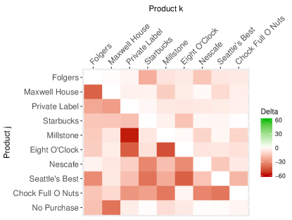
Figure 9: Illustration of the substitution/complementarity matrices $\boldsymbol{\Delta}^{\text{avg}}$ on coffee brands, corresponding to the decision forest model (left) and the ranking-based model (right).

Figure 9 shows that the decision forest model and the ranking-based model capture similar substitution patterns. For example, both models show that, on average, the choice probabilities of Millstone and Eight O’Clock decrease by about 60% and 40%, respectively, when Private Label is added, as shown in elements (5,3) and (6,3) from the top-left corner. However, since the ranking-based model satisfies the regularity property, all elements in $\boldsymbol{\Delta}^{\text{avg}}$ are forced to be non-positive. Thus, with the ranking-based model we are restricted to understanding only the substitution behavior between products, and we cannot use it to identify any complementarity behavior.

In contrast, the decision forest model is not constrained by the regularity property, and thus we can use it to identify interesting complementarities between certain brands. For example, Figure 9 shows that adding Seattle’s Best to the assortment increases the choice probability of Starbucks by about 25% on average; the addition of Eight O’Clock provides a similar boost of about 16% to the choice probability of Maxwell House.

Another way to identify substitution and complementarity effects between products is to directly inspect the decision forest model. Figure 10 visualizes the top three trees by $\lambda_{t}$ value of the decision forest model used in the left hand matrix of Figure 9. The second tree exhibits the decoy effect that is described in Section 3.5. This customer type behaves in the following way: when Eight O’Clock exists in the assortment, the customer will purchase Maxwell House if it is available; otherwise, if Eight O’Clock does not exist in the assortment, the customer will purchase Private Label if it is available. This matches the complementarity effect shown in Figure 9 (element (2,6) in the left-hand matrix). The decision forest model is also capable of capturing effects that do not fit into well-studied customer behaviors in the marketing literature. For example, the first tree in Figure 10 corresponds to customers who purchase Millstone only if Eight O’Clock is observed in the assortment; otherwise, they do not make a purchase. Similarly, the third tree represents a decoy-like effect, where a customer checks for the existence of Starbucks: if it exists, the customer will purchase Starbucks if Seattle’s Best is available; if not, the customer will purchase Maxwell House if it is available. This highlights another benefit of our nonparametric approach: since we do not impose any assumptions on how the data is generated, we are able to discover interesting customer behaviors that fall outside of well-studied irrational behaviors.

Figure 10: Top three decision trees on coffee brands with highest probability weights in the decision forest model learned from data. From left to right, the probability weights ($\lambda_{t}$ values) are $4.1\%$, $2.5\%$, and $2.3\%$, respectively.

7 Conclusions

In this paper, we proposed the decision forest model, which can model any discrete choice behavior, regardless of whether it belongs to the RUM class or not. Given data in the form of a collection of historical assortments, we proved that simple trees, whose depth scales logarithmically and leaf complexity scales linearly with the number of assortments, are sufficient to fit the data. We further proposed two practical estimation methods for learning the decision forest model from historical assortments. Through experiments with real data, we showed that the decision forest model generally outperforms other rational and non-rational models in out-of-sample prediction in the presence of non-rational customer behavior, and can be used to generate insights on the complementarity/substitution behaviors between products. We hope that this work will encourage the further exploration of data-driven methodologies in the non-rational choice modeling space.

The authors sincerely thank the department editor Chung-Piaw Teo, the associate editor and two anonymous reviewers for their thoughtful comments and feedback that have helped to significantly improve the paper. The authors also thank Huseyin Topaloglu for helpful feedback and being the discussant of this paper at the 2019 INFORMS Revenue Management and Pricing Conference. The authors gratefully acknowledge Information Resources Inc. (IRI) and the authors of Bronnenberg et al. (2008) for the IRI Academic Data Set that was used in Section 6. Any findings expressed in this paper are those of the authors and do not necessarily reflect the views of IRI.

Electronic companion for “Decision Forest: A Nonparametric Approach to Modeling Irrational Choice”

8 Proofs

8.1 Proof of Proposition 3.1

For each ranking $\sigma_{j}$, $j=1,2,\ldots,m$, we can write down its preference order explicitly as $\sigma_{j}=\{p^{(j)}_{1}\succ p^{(j)}_{2}\succ\ldots\succ p^{(j)}_{K_{j}}\succ 0\}$, where $a\succ b$ denotes that $a$ is preferred to $b$; for this ranking, $K_{j}$ products are preferred over the no-purchase option, and product $p^{(j)}_{1}$ is the most preferred. Assume each ranking $\sigma_{j}$ has probability weight $\lambda_{j}$. Now we construct the forest $F$ as follows: for $j=1,\ldots,m$, we build a decision tree $t_{j}$ with the structure shown in Figure 11. Additionally, we associate tree $t_{j}$ with probability $\lambda_{j}$. Note that ranking $\sigma_{j}=\{p^{(j)}_{1}\succ p^{(j)}_{2}\succ\ldots\succ p^{(j)}_{K_{j}}\succ 0\}$ and the decision tree in Figure 11 give the same decision process: if product $p^{(j)}_{1}$ is in the assortment, we buy it; otherwise, if product $p^{(j)}_{1}$ is not in the assortment but $p^{(j)}_{2}$ is, we buy $p^{(j)}_{2}$; otherwise, if both $p^{(j)}_{1}$ and $p^{(j)}_{1}$ are not in assortment but $p^{(j)}_{3}$ is, we buy $p^{(j)}_{3}$; and so on. Therefore, for any option $o$ and any assortment $S$, we have

$$\mathbf{P}^{(F,{\lambda})}(o\mid S) =\sum_{j=1}^{m}\lambda_{j}\cdot\mathbb{I}\{o=\hat{A}(S,t_{j})\}$$

$$=\sum_{j=1}^{m}\lambda_{j}\cdot\mathbb{I}\{\text{ranking }\sigma_{j}\text{ selects option }o\text{ given }S\}$$

$$=\mathbf{P}^{(\Sigma,\boldsymbol{\lambda})}(o\mid S),$$

where the second equality comes from the fact that ranking $\sigma_{i}$ and tree $t_{i}$ makes same decision given $S$, and the third equality is from the definition of the ranking-based model. $\Halmos$

Figure 11: Ranking $\sigma_{j}=\{p^{(j)}_{1}\succ p^{(j)}_{2}\succ\ldots\succ p^{(j)}_{K_{j}}\succ 0\}$ can be represented as a purchase decision tree.

8.2 Proof of Theorem 3.2

We prove the theorem by constructing a forest $F$ consisting of $(N+1)^{2^{N}}$ balanced trees. We first define the common structure of each tree in the forest. Each tree $t$ in the forest has depth $N+1$ and shares the following structure for first the $N$ levels:

$$x_{s}=1,\quad\forall\ s\in\mathbf{splits}(t)\ \text{such that}\ \textrm{dist}(r(t),s)=0,$$ (13)

$$x_{s}=2,\quad\forall\ s\in\mathbf{splits}(t)\ \text{such that}\ \textrm{dist}(r(t),s)=1,$$ (14)

$$x_{s}=3,\quad\forall\ s\in\mathbf{splits}(t)\ \text{such that}\ \textrm{dist}(r(t),s)=2,$$ (15)

$$\vdots$$

$$x_{s}=N,\quad\forall\ s\in\mathbf{splits}(t)\ \text{such that}\ \textrm{dist}(r(t),s)=N-1,$$ (16)

In words, the root split node $r(t)$ checks for the existence of product $1$ in the assortment; the split nodes in the second level of the tree (those with $\textrm{dist}(r(t),s)=1$) check for product 2; the split nodes in the third level check for product $3$; and so on, all the way to the $N$th level, at which all splits node check for product $N$. Figure 12 provides an example of this tree structure for $N=3$. In this tree, the left-most leaf node corresponds to assortment $S=\{1,2,3\}$, the second leaf node from the left corresponds to assortment $S=\{1,2\}$, and so on, until the right-most leaf which corresponds to the empty assortment ($S=\emptyset$).

Figure 12: An example of the structure of the trees in the forest needed for the proof of Theorem 3.2 for $N=3$.

In this tree structure, there are exactly $2^{N}$ leaf nodes, which we will index from left to right as $l_{1},\ldots,l_{2^{N}}$. Note that each leaf node of a tree in $F$ has a one-to-one correspondence with one of the $2^{N}$ possible assortments of the products.

To specify the leaves, we require some additional definitions. Let us denote the $2^{N}$ possible assortments of the $N$ products by $S_{1},S_{2},\dots,S_{2^{N}}$, in correspondence with the leaf nodes $l_{1},\ldots,l_{2^{N}}$, respectively. For the leaves $\ell_{1},\dots,\ell_{2^{N}}$, we use $o_{1},o_{2},\dots,o_{2^{N}}$ to denote the purchase decisions associated with those leaves, and we use $\mathbf{o}=(o_{1},\dots,o_{2^{N}})$ to denote the $2^{N}$-tuple of purchase decisions. Let $\mathbf{o}^{1},\dots,\mathbf{o}^{(N+1)^{2^{N}}}$ be a complete enumeration of the $(N+1)^{2^{N}}$ possible $2^{N}$-tuples of the purchase decisions from $\prod_{i=1}^{2^{N}}\mathcal{N}^{+}$.

With these definitions, we define our forest $F$ as consisting of $(N+1)^{2^{N}}$ trees, where each tree follows the structure in equations (13)–(16), each tree is indexed from $t=1$ to $t=(N+1)^{2^{N}}$ and the purchase decisions of the leaves in tree $t$ are given by the tuple $\mathbf{o}^{t}$ as defined above. We define the probability distribution $\boldsymbol{\lambda}=(\lambda_{1},\dots,\lambda_{(N+1)^{2^{N}}})$ by defining the probability $\lambda_{t}$ of each tree $t$ as:

$$\lambda_{t}=\prod_{j=1}^{2^{N}}\mathbf{P}(o^{t}_{j}\mid S_{j}).$$ (17)

It is straightforward to verify that $\boldsymbol{\lambda}$ is nonnegative and sums to one. Before continuing, we note that not all of the trees defined in this way will satisfy Requirement 2 from Section 3.2, which requires that the purchase decision in each leaf must be consistent with the products along the path of splits from the root node to the leaf; in other words, for some trees $o^{t}_{j}$ will not be contained in $S_{j}$. However, for any tree where this is the case, by the definition in equation (17), the corresponding $\lambda_{t}$ will be zero because $\mathbf{P}(o^{t}_{j}\mid S_{j})$ is zero whenever $o^{t}_{j}\notin S_{j}$. Thus, those trees can be safely removed from $F$ without changing the overall model.

We now show that the decision forest model $(F,\boldsymbol{\lambda})$ outputs the same choice probabilities as the true model $\mathbf{P}(\cdot\mid\cdot)$. For any assortment $S_{i}$ and option $o$, we have

$$\mathbf{P}^{(F,\lambda)}(o\mid S_{i})$$

$$=\sum_{t=1}^{(N+1)^{2^{N}}}\lambda_{t}\cdot\mathbb{I}\{o=\hat{A}(S_{i},t)\}$$

$$=\sum_{t\,:\,o^{t}_{i}=o}\lambda_{t}$$

$$=\sum_{t\,:\,o^{t}_{i}=o}\ \prod_{i^{\prime}=1}^{2^{N}}\mathbf{P}(o^{t}_{i^{\prime}}\mid S_{i^{\prime}})$$

$$=\sum_{o_{1}=0}^{N}\cdots\sum_{o_{i-1}=0}^{N}\sum_{o_{i+1}=0}^{N}\cdots\sum_{o_{2^{N}}=0}^{N}\mathbf{P}(o_{1}\mid S_{1})\cdots\mathbf{P}(o_{i-1}\mid S_{i-1})\cdot\mathbf{P}(o\mid S_{i})\cdot\mathbf{P}(o_{i+1}\mid S_{i+1})\cdots\mathbf{P}(o_{2^{N}}\mid S_{2^{N}})$$

$$=\mathbf{P}(o\mid S_{i})\left[\sum_{o_{1}=0}^{N}\mathbf{P}(o_{1}\mid S_{1})\right]\cdots\left[\sum_{o_{i-1}=0}^{N}\mathbf{P}(o_{i-1}\mid S_{i-1})\right]\left[\sum_{o_{i+1}=0}^{N}\mathbf{P}(o_{i+1}\mid S_{i+1})\right]\cdots\left[\sum_{o_{2^{N}}=0}^{N}\mathbf{P}(o_{2^{N}}\mid S_{2^{N}})\right]$$

$$=\mathbf{P}(o\mid S_{i}),$$

where the first equality follows from how choice probabilities under the decision forest model are defined in equation (3); the second follows from how our forest is constructed and how the $\mathbf{o}^{t}$ tuples are defined; the third equality follows from the definition of $\boldsymbol{\lambda}$; the fourth from the definition of the $\mathbf{o}^{t}$ tuples; the fifth by algebra; and the last by recognizing that the choice probabilities for a given assortment must sum to one.

8.3 Proof of Theorem 4.1

Before we prove Theorem 4.1, we establish three useful lemmas. Some of the results will be also used in the proof of Theorem 4.2 in Section LABEL:subsec:appendix_proof_thm:asymptotic_size_of_forest.

Lemma 8.1

For any decision tree $t$ that satisfies Requirements 1 and 2 in Section 3.2, there exists a purchase decision tree $t^{\prime}$ such that:

1. Tree $t^{\prime}$ satisfies Requirement 1, 2 and 3;

2. Tree $t$ and $t^{\prime}$ have same purchase decision under any given assortment; and

3. $\mathrm{Depth}(t^{\prime})\leq\mathrm{Depth}(t)$ and $|\mathbf{leaves}(t^{\prime})|\leq|\mathbf{leaves}(t)|$.

Proof 8.2

Proof of Lemma 8.1: Let $t$ be a tree that does not satisfy Requirement 3, and consider the following procedure:

1. Select any leaf $\ell\in\mathbf{leaves}(t)$ for which Requirement 3 is violated. Let $path(\ell)\equiv\{s_{1},s_{2},\ldots,s_{d-1}\}$ be the sequence of splits from root $r(t)\equiv s_{1}$ to $s_{d-1}$, which is the parent node of $\ell$. Let $i\in\mathcal{N}$ be a product encountered at least two times as the decision process traverses $path(\ell)$. Let $s_{u_{1}},s_{u_{2}},\ldots,s_{u_{e_{i}}}$, where $u_{1}<u_{2}<\dots<u_{e_{i}}$, be the subsequence of split nodes associated with product $i$ in $path(\ell)$. (Note that $e_{i}\geq 2$.)

2. If $s_{u_{1}}\in\textbf{LS}(\ell)$, then remove all right subtrees branched at $s_{u_{2}},\ldots,s_{u_{e_{i}}}$ from $t$. Otherwise, if $s_{u_{1}}\in\textbf{RS}(\ell)$, then remove all left subtrees branched at $s_{u_{2}},\ldots,s_{u_{e_{i}}}$ from $t$.

3. Delete split nodes $s_{u_{2}},\ldots,s_{u_{e_{i}}}$ from tree $t$, and “glue” the remaining pieces by setting $s_{u_{j}-1}$ as the parent node of the remaining child node of $s_{u_{j}}$ for $j=2,\ldots,e_{i}$.

Consider now applying steps 1 - 3 repeatedly to tree $t$, until all of the leaves in the tree satisfy Requirement 3; let the resulting tree be denoted by $t^{\prime}$. Note that we are guaranteed to terminate with such a tree, because each time we apply steps 1 - 3, we delete at least one subtree from the tree (and thus at least one leaf), and the tree contains finitely many leaves. In addition to Requirement 3, steps 1 - 3 also preserve Requirements 1 and 2. Thus, tree $t^{\prime}$ satisfies condition (1) of the lemma.

Note also that for a given tree, the tree we obtain after applying steps 1 - 3 is equivalent to that initial tree, in that any assortment is mapped by the two trees to the same purchase decision. This is true because the leaves within the subtrees that are removed are leaves that are unreachable (i.e., there does not exist an assortment that can reach them). For example, if ${}_{u_{1}}\in\textbf{LS}(\ell)$, then any leaf in the right subtree branched at $s_{u_{2}},\ldots,s_{u_{e_{i}}}$ is such that product $i$ must be in the assortment and not in the assortment in order to reach the leaf, which is impossible. Thus, tree $t^{\prime}$ satisfies condition (2) of the lemma.

Lastly, since steps 1 - 3 involve deleting subtrees and splits and re-attaching the disconnected pieces, tree $t^{\prime}$ is no deeper than tree $t$ and has no more leaves than tree $t$, thus verifying condition (3) of the lemma.

Lemma 8.1 plays an important role in the proofs of Theorem 4.1 and 4.2. In fact, we prove both theorems by directly constructing decision forest models. However, the trees in the forest may violate Requirement 3 in Section 3.2. If such violation happens on a tree $t$, we will use Lemma 8.1 to find an equivalent tree $t^{\prime}$ that satisfies Requirement 3 without increasing either the depth or the number of leaves, and replace $t$ by $t^{\prime}$ in the forest. For convenience, we summarize the procedure in Lemma 8.1 as the following algorithm.

Algorithm 4 Modifying a tree of Requirements 1 and 2 to satisfy Requirement 3 in Section 3.2

.

1:procedure TreeModification(a tree $t$ that satisfies Requirements 1 and 2)

2:     while there exists a leaf $\ell\in\mathbf{leaves}(t)$ violates Requirement 3 do

3:         Set $path(\ell)\leftarrow\{s_{1},s_{2},\ldots,s_{d-1}\}$ (see the definition in the proof of Lemma 8.1).

4:         Set $i\leftarrow\arg\max_{k\in\mathcal{N}}\sum_{j=1}^{d-1}\mathbb{I}\{k=x_{s_{j}}\}.$

5:         Set $\{u_{1}<u_{2}<\ldots<u_{e_{i}}\}\leftarrow\{j\mid x_{s_{j}}=i,j\in\{1,2,\ldots,d-1\}\}$.

6:         if $s_{u_{1}}\in\textbf{LS}(\ell)$ then

7:              Remove all right subtrees branched at $s_{u_{2}},\ldots,s_{u_{e_{i}}}$ from tree $t$.

8:         else

9:              Remove all left subtrees branched at $s_{u_{2}},\ldots,s_{u_{e_{i}}}$ from tree $t$.          

10:         for $w=e_{i},e_{i}-1,\ldots,2$ do

11:              Delete split node $s_{w}$.

12:              Set the remaining child node of $s_{w}$ as the child node of $s_{w-1}$.               

13:     return $t$

Our next result, Lemma 8.3 states that a data set of a single assortment can be perfectly fit by a depth 2 decision forest.

Lemma 8.3

For any dataset $\mathcal{S}$ consisting of only one assortment $S$, there exists a forest $F$ of depth $2$ and of leaf complexity $2$ and a probability distribution $\boldsymbol{\lambda}$ over $F$ such that $\mathbf{P}^{(F,\boldsymbol{\lambda})}(o\mid S)=v_{o,S}$ for every $o\in\mathcal{N}^{+}$.

References

- Alptekinoğlu and Semple [2016] A. Alptekinoğlu and J. H. Semple. The exponomial choice model: A new alternative for assortment and price optimization. Operations Research, 64(1):79–93, 2016.
- Aouad et al. [2015] A. Aouad, V. F. Farias, and R. Levi. Assortment optimization under consider-then-choose choice models. Available at SSRN 2618823, 2015.
- Aouad et al. [2018a] A. Aouad, V. Farias, R. Levi, and D. Segev. The approximability of assortment optimization under ranking preferences. Operations Research, 66(6):1661–1669, 2018a.
- Aouad et al. [2018b] A. Aouad, J. Feldman, and D. Segev. The exponomial choice model: Algorithmic frameworks for assortment optimization and data-driven estimation case studies. Available at SSRN 3192068, 2018b.
- Ariely [2008] D. Ariely. Predictably Irrational. HarperCollins New York, 2008.
- Ben-Akiva and Lerman [1985] M.E. Ben-Akiva and S.R. Lerman. Discrete Choice Analysis: Theory and Application to Travel Demand. MIT press, 1985.
- Berbeglia [2018] G. Berbeglia. The generalized stochastic preference choice model. arXiv preprint arXiv:1803.04244, 2018.
- Bertsimas and Mišić [2019] D. Bertsimas and V. V. Mišić. Exact first-choice product line optimization. Operations Research, 67(3):651–670, 2019.
- Blanchet et al. [2016] J. Blanchet, G. Gallego, and V. Goyal. A markov chain approximation to choice modeling. Operations Research, 64(4):886–905, 2016.
- Block and Marschak [1959] H. D. Block and J. Marschak. Random orderings and stochastic theories of response. Technical report, Cowles Foundation for Research in Economics, Yale University, 1959.
- Breiman [2001] L. Breiman. Random forests. Machine Learning, 45(1):5–32, 2001.
- Breiman et al. [1984] L. Breiman, J. Friedman, C. J. Stone, and R. A. Olshen. Classification and regression trees. CRC press, 1984.
- Bronnenberg and Mela [2004] B. J. Bronnenberg and C. F. Mela. Market roll-out and retailer adoption for new brands. Marketing Science, 23(4):500–518, 2004.
- Bronnenberg et al. [2008] B. J. Bronnenberg, M. W. Kruger, and C. F. Mela. Database paper—the IRI marketing data set. Marketing science, 27(4):745–748, 2008.
- Calafiore and Campi [2005] G. Calafiore and M. Campi. Uncertain convex programs: randomized solutions and confidence levels. Mathematical Programming, 102(1):25–46, 2005.
- Chen and Guestrin [2016] T. Chen and C. Guestrin. Xgboost: A scalable tree boosting system. In Proceedings of the 22nd ACM SIGKDD International Conference on Knowledge Discovery and Data Mining, pages 785–794. ACM, 2016.
- Désir et al. [2015a] A. Désir, V. Goyal, D. Segev, and C. Ye. Capacity constrained assortment optimization under the markov chain-based choice model. Operations Research, 2015a. Forthcoming.
- Désir et al. [2015b] A. Désir, V. Goyal, H. Topalogu, and J. Zhang. Robust assortment optimization under the markov chain model. Technical report, Working Paper, 2015b.
- Dogan and Yildiz [2018] S. Dogan and K. Yildiz. Choice through a unified lens: The prudential model. Available at SSRN 3085542, 2018.
- Echenique and Saito [2015] F. Echenique and K. Saito. General Luce model. Economic Theory, pages 1–16, 2015.
- Echenique et al. [2018] F. Echenique, K. Saito, and G. Tserenjigmid. The perception-adjusted Luce model. Mathematical Social Sciences, 93:67–76, 2018.
- Farias et al. [2013] V. F. Farias, S. Jagabathula, and D. Shah. A nonparametric approach to modeling choice with limited data. Management science, 59(2):305–322, 2013.
- Feldman et al. [2018] J. Feldman, A. Paul, and H. Topaloglu. Assortment optimization with small consideration sets. Operations Research, 2018. Forthcoming.
- Feldman and Topaloglu [2017] J. B. Feldman and H. Topaloglu. Revenue management under the markov chain choice model. Operations Research, 65(5):1322–1342, 2017.
- Ferreira et al. [2015] K. J. Ferreira, B. H. A. Lee, and D. Simchi-Levi. Analytics for an online retailer: Demand forecasting and price optimization. Manufacturing & Service Operations Management, 18(1):69–88, 2015.
- Freund and Schapire [1996] Y. Freund and R. Schapire. Experiments with a new boosting algorithm. In Machine Learning: Proceedings of the Thirteenth International Conference, pages 148–156. Morgan Kauffman, San Francisco, CA, 1996.
- Friedman [2001] J. H. Friedman. Greedy function approximation: a gradient boosting machine. Annals of statistics, pages 1189–1232, 2001.
- Gallego et al. [2014] G. Gallego, R. Ratliff, and S. Shebalov. A general attraction model and sales-based linear program for network revenue management under customer choice. Operations Research, 63(1):212–232, 2014.
- Golrezaei et al. [2014] N. Golrezaei, H. Nazerzadeh, and P. Rusmevichientong. Real-time optimization of personalized assortments. Management Science, 60(6):1532–1551, 2014.
- Hauser [2014] J. R. Hauser. Consideration-set heuristics. Journal of Business Research, 67(8):1688–1699, 2014.
- Horan [2011] S. Horan. Choice by tournament. Technical report, Working paper, Boston University., 2011.
- Huber et al. [1982] J. Huber, J. W. Payne, and C. Puto. Adding asymmetrically dominated alternatives: Violations of regularity and the similarity hypothesis. Journal of consumer research, 9(1):90–98, 1982.
- Jagabathula and Rusmevichientong [2016] S. Jagabathula and P. Rusmevichientong. A nonparametric joint assortment and price choice model. Management Science, 63(9):3128–3145, 2016.
- Jagabathula and Rusmevichientong [2019] S. Jagabathula and P. Rusmevichientong. The limit of rationality in choice modeling: Formulation, computation, and implications. Management Science, 65(5):2196–2215, 2019.
- Kahneman and Tversky [1979] D. Kahneman and A. Tversky. Prospect theory: An analysis of decision under risk. Econometrica, 47(2):263–292, 1979.
- Li and Tang [2017] J. Li and R. Tang. Every random choice rule is backwards-induction rationalizable. Games and Economic Behavior, 104:563–567, 2017.
- Maragheh et al. [2018] R. Y. Maragheh, A. Chronopoulou, and J. M. Davis. A customer choice model with HALO effect. arXiv preprint arXiv:1805.01603, 2018.
- McFadden and Train [2000] D. McFadden and K. Train. Mixed MNL models for discrete response. Journal of Applied Econometrics, 15(5):447–470, 2000.
- Mishra et al. [2014] V. K. Mishra, K. Natarajan, D. Padmanabhan, C.-P. Teo, and Xiaobo Li. On theoretical and empirical aspects of marginal distribution choice models. Management Science, 60(6):1511–1531, 2014.
- Mišić [2016] V. V. Mišić. Data, models and decisions for large-scale stochastic optimization problems. PhD thesis, Massachusetts Institute of Technology, 2016.
- Mišić [2020] V. V. Mišić. Optimization of tree ensembles. Operations Research, 68(5):1605–1624, 2020.
- Moosmann et al. [2007] F. Moosmann, B. Triggs, and F. Jurie. Fast discriminative visual codebooks using randomized clustering forests. In Advances in neural information processing systems, pages 985–992, 2007.
- Natarajan et al. [2009] K. Natarajan, M. Song, and C.-P. Teo. Persistency model and its applications in choice modeling. Management Science, 55(3):453–469, 2009.
- Nijs et al. [2007] V. R. Nijs, S. Srinivasan, and K. Pauwels. Retail-price drivers and retailer profits. Marketing Science, 26(4):473–487, 2007.
- Poundstone [2010] W. Poundstone. Priceless: The myth of fair value (and how to take advantage of it). Hill and Wang, 2010.
- Quinlan [1986] J. R. Quinlan. Induction of decision trees. Machine learning, 1(1):81–106, 1986.
- Quinlan [1993] J. R. Quinlan. C4.5: Programs for machine learning. Morgan Kaufmann, San Francisco, CA, 1993.
- Rahimi and Recht [2008] A. Rahimi and B. Recht. Random features for large-scale kernel machines. In Advances in neural information processing systems, pages 1177–1184, 2008.
- Rahimi and Recht [2009] A. Rahimi and B. Recht. Weighted sums of random kitchen sinks: Replacing minimization with randomization in learning. In Advances in neural information processing systems, pages 1313–1320, 2009.
- Rieskamp et al. [2006] J. Rieskamp, J. R. Busemeyer, and B. A. Mellers. Extending the bounds of rationality: Evidence and theories of preferential choice. Journal of Economic Literature, 44(3):631–661, 2006.
- Simonson [1989] I. Simonson. Choice based on reasons: The case of attraction and compromise effects. Journal of consumer research, 16(2):158–174, 1989.
- Şimşek and Topaloglu [2018] A. S. Şimşek and H. Topaloglu. An expectation-maximization algorithm to estimate the parameters of the markov chain choice model. Operations Research, 66(3):748–760, 2018.
- Train [2009] K. E. Train. Discrete choice methods with simulation. Cambridge university press, 2009.
- Tversky [1969] A. Tversky. Intransitivity of preferences. Psychological review, 76(1):31, 1969.
- Tversky [1972] A. Tversky. Elimination by aspects: A theory of choice. Psychological review, 79(4):281, 1972.
- Tversky and Simonson [1993] A. Tversky and I. Simonson. Context-dependent preferences. Management science, 39(10):1179–1189, 1993.
- van Ryzin and Vulcano [2014] G. van Ryzin and G. Vulcano. A market discovery algorithm to estimate a general class of nonparametric choice models. Management Science, 61(2):281–300, 2014.
- van Ryzin and Vulcano [2017] G. van Ryzin and G. Vulcano. An expectation-maximization method to estimate a rank-based choice model of demand. Operations Research, 65(2):396–407, 2017.
- Xu and Zhou [2007] Y. Xu and L. Zhou. Rationalizability of choice functions by game trees. Journal of Economic theory, 134(1):548–556, 2007.