North–South Asymmetry in Solar Activity and Solar Cycle Prediction, IV: Prediction for Lengths of Upcoming Solar Cycles

Abstract

We analyzed the daily sunspot-group data reported by the Greenwich Photoheliographic Results (GPR) during the period 1874 – 1976 and Debrecen Photoheligraphic Data (DPD) during the period 1977 – 2017 and studied North–South asymmetry in the maxima and minima of the Solar Cycles 12 – 24. We derived the time-series of the 13-month smoothed monthly mean corrected whole-spot areas of the sunspot groups in the Sun’s whole sphere (WSGA), northern hemisphere (NSGA), and southern hemisphere (SSGA). From these smoothed time series we obtained the values of the maxima and minima, and the corresponding epochs, of the WSGA, NSGA, and SSGA Cycles 12 – 24. We find that there exists a 44 – 66 years periodicity in the North–South asymmetry of minimum. A long periodicity (130 – 140 years) may exist in the asymmetry of maximum. A statistically significant correlation exists between the maximum of SSGA Cycle $n$ and the rise time of WSGA Cycle $n+2$. A reasonably significant correlation also exists between the maximum of WSGA Cycle $n$ and the decline time of WSGA Cycle $n+2$. These relations suggest that the solar dynamo carries memory over at least three solar cycles. Using these relations we obtained the values $11.7\pm 0.15$ years, $11.2\pm 0.2$ years, and $11.45\pm 0.3$ years for the lengths of WSGA Cycles 24, 25, and 26, respectively, and hence, July 2020, October 2031, and March 2043 for the minimum epochs (start dates) of WSGA Cycles 25, 26, and 27, respectively. We also obtained May 2025 and March 2036 for the maximum epochs of WSGA Cycles 25 and 26, respectively. It seems during the late Maunder Minimum sunspot activity was absent around the epochs of the maxima of NSGA-cycles and the minima of SSGA-cycles, and some activity was present at the epochs of the maxima of some SSGA-cycles and the minima of some NSGA-cycles.

1 Introduction

North–South asymmetry in solar activity may have some important implications for the solar-dynamo mechanism ($e.g.$ soko94; bd13; shetye15). Therefore, a study of variations in the North–South asymmetry of solar activity may be useful for better understanding the underlying mechanism of the solar cycle. Besides a 11 – 12-year periodicity (carb93; jg97a) and many short periodicities (vizo90; chow13; rj15, and references therein), the existence of a $\approx$110-year periodicity (verma93) in the North-South asymmetry of solar activity is known. It is well known that large and small sunspot groups (in general active regions) have different physical origin (pf72; gf79; howard96; jg97b; kmh02; siva03). Recently, short-term periodicities in the variations of the North–South asymmetry in the numbers of different-size sunspot groups have also been studied (mb16). verma93 has found the $\approx$110-year periodicity in the North–South asymmetry of solar activity by using the combined data of many different indices of solar activity that were available for different periods: sunspot area (1832 – 1976), sunspot counts (1833 – 1877), sunspot groups (1954 – 1986), solar flares (1936 – 1954), major flares (1955 – 1979), gamma-ray flares (1980 – 1986), and H$\alpha$ flares (1987 – 1990). Here we study the long-term variation in the North–South asymmetry of solar activity by using the 143 years of updated GPR and DPD sunspot group data, $i.e.$ by using the data of a single activity index. The average value of the areas of sunspot groups in the solar maximum is much larger than that of the sunspot groups in the solar minimum. In addition, it seems the maxima and minima of solar cycles comprise relatively strong quadrupole and dipole magnetic fields, respectively ($e.g.$ dbh12). Hence, the cycle-to-cycle modulations in maximum and minimum could be different and may have different implications on the solar dynamo. Therefore, here we have examined the long-term variations in the North–South asymmetry of solar maximum and minimum, independently.

Prediction of the properties of solar cycles is important for understanding the underlying mechanism of the solar cycle. Prediction of the amplitude and the length (period) of a solar cycle is important also for monitoring space weather and for understanding the solar–terrestrial relationship. A wide range of techniques have been used for prediction of the amplitude of a solar cycle (kane07; pes08; obrid08; hath15). Although the average cycle length can be fairly accurately determined (hath15), so far no technique is available to make prediction of the maximum epoch and length of a cycle. By using the well-known Waldmeier effect (wald35; wald39; hath15), $i.e.$ inverse relationship between the amplitude of a cycle and its rise time (the time taken for rising from minimum to maximum), it is only possible to make an approximate prediction for the rise time of a cycle from a predicted amplitude. The existence of an approximate inverse relationship between the amplitude of a cycle and its length (time from the minimum of a cycle to the minimum of next cycle) is also well-known (hs97; solanki02). By using this relationship it is only possible to make an approximate prediction for the length of a cycle from the known/predicted amplitude.

The solar rotational and meridional flows may cause the magnetic fields at different heliographic latitudes during different time intervals of a solar cycle to contribute to the activity at the same or different heliographic latitudes during the following cycle(s). Hence, in our earlier articles (Article I : jj07, Article II: jj08, and Article III: jj15) the combined Greenwich and Solar Optical Observing Network (SOON) sunspot-group data during 1874 – 2013 were analyzed and correlations of different latitude bands of activity (sums of the areas of sunspot groups) with the amplitude of solar cycle were determined. It was found that the sums of the areas of the sunspot groups in the $0^{\circ}$ – $10^{\circ}$ latitude interval of the Sun’s northern hemisphere and in the time interval of $-1.35$ year to $+2.15$ year from the time of the preceding minimum of a sunspot cycle, and also in the same latitude interval of the southern hemisphere but $+1.0$ year to $+1.75$ year from the time of the maximum of a sunspot cycle, correlate well with the amplitude (maximum of the 13-month smoothed monthly sunspot number) of its immediate following cycle. This enabled us to made predictions for the amplitude of Solar Cycle 24 (jj07, 2008), and that of Cycle 25 (jj15). Our predictions ($74\pm 10$ and $87\pm 7$) for the amplitude of Cycle 24 closely agree with the observed amplitude (81.9). We have predicted $50\pm 10$ for the amplitude of Solar Cycle 25 (jj15).

A number of authors predicted the amplitude and the maximum epoch of Cycle 25 by using various techniques (pk18; sarp18, and references therein). Some authors predicted a high amplitude (up to $\approx$150) and some others predicted a low ($\approx$50) amplitude and years 2023 – 2025 for the maximum epoch of this cycle. Here we have attempted to predict the maximum epochs of Solar Cycles 25 and 26 and the lengths of Cycles 24, 25, and 26. As mentioned above, in our earlier articles we have used the North–South asymmetry in the latitude distribution of sunspot activity. Here, we used the North–South asymmetry property of the maxima and minima of the solar cycles. However, the physical mechanism (flux-transport-processes) behind both our earlier and present methods is same.

In the next section we describe the data analysis, in Section 3 we present the results, and in Section 4 we summarize the conclusions and discuss briefly.

2 Data analysis

The daily data of sunspot groups in the Greenwich Photoheliographic Results (GPR) during the period April 1874 – December 1976 and Debrecen Photoheliographic data (DPD) during the period January 1977 – June 2017 are downloaded from fenyi.solarobs.unideb.hu/pub/DPD/ (for details see gyr10). These data contain the date with time, heliographic latitude and longitude, corrected whole-spot area [A] in millionth of solar hemisphere (msh), central meridian distance, etc. of each of the sunspot groups observed on each day. The time series of the 13-month smoothed monthly mean values of the international sunspot number $R_{\rm Z}$ (ISSN) and that of the corresponding revised sunspot number (SN) during the period 1874 – 2017 are downloaded from www.sidc.be/silso/datafiles (Source: WDC-SILSO, Royal Observatory of Belgium, Brussels). From the 13-month smoothed monthly mean $R_{\rm Z}$-values we obtained the maximum [$R_{\rm M}$] and minimum [$R_{\rm m}$] values of the Sunspot (ISSN) Cycles 12 – 24 and their corresponding epochs. We determined separate time series of 13-month smoothed monthly mean corrected whole-spot areas of the sunspot groups occurred in the Sun: whole sphere (WSGA), northern hemisphere (NSGA), and southern hemisphere (SSGA), in exactly the same way as the corresponding smoothed time series of $R_{\rm Z}$ are determined. That is, first we determined the average value of the corrected areas of whole sunspot groups in each of the classes WSGA, NSGA, and SSGA for each calender month of each year during the period 1874 – 2017, and then we determined the corresponding time series of 13-month smoothed monthly mean values. From these smoothed time series we obtained the values of the maxima and minima, and their corresponding epochs, of the WSGA, NSGA, and SSGA Cycles 12 – 24. We also determined the rise times of all the Cycles 12 – 24, and the decline times and the lengths of the Cycles 12 – 23. The North–South asymmetry in the maximum value and that in the minimum value of each cycle are calculated. The epochs of the maxima and minima of the cycles of $R_{\rm Z}$ and the sunspot area are not exactly the same in the case of some solar cycles ($e.g.$ ramesh08). In fact, dgt08 found that Waldmeier effect is not present in the case of solar cycles in the area of sunspot groups. In an earlier analysis (jj12) we found that for many cycles the positions of the maxima of the small, large (medium-sized), and very-large sunspot groups are different and also considerably different from the corresponding ISSN maxima. Therefore, from the 13-month smoothed monthly mean time series we have determined the values of the actual maximum [$A_{\rm M}$] and minimum [$A_{\rm m}$] and their corresponding epochs, and also the values [$A^{*}_{\rm M}$ and $A^{*}_{\rm m}$] corresponding to the epochs of maximum [$R_{\rm M}$] and minimum [$R_{\rm m}$] of the ISSN cycle. To make predictions for the rise times and the lengths of the upcoming solar cycles we study cross-correlations among the parameters of the WSGA, NSGA, and SSAG cycles. All of the aforementioned calculations were done by using the epochs of $R_{\rm M}$ and $R_{\rm m}$ of the sunspot cycles obtained from both the original (ISSN) and the revised (SN) time series. However, the results correspond to the epochs of $R_{\rm M}$ and $R_{\rm m}$ of the revised and the original time series were found to be almost the same. Hence, in the next section we report the results derived by using the original time series only.

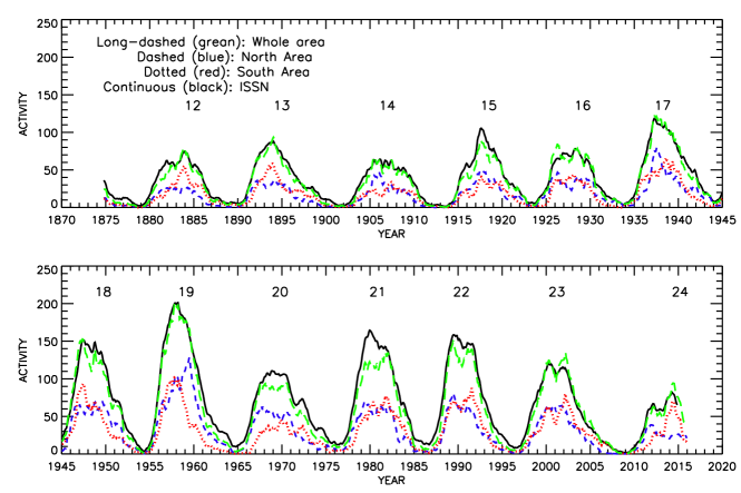
Figure 1.: Variations in the 13-month smoothed monthly mean area of sunspot groups in the whole hemisphere: WSGA (green-long-dashed curve), northern hemisphere: NSGA (blue-dashed curve), southern hemisphere: SSGA (red-dotted curve), and international sunspot number (ISSN) $R_{\rm{}_{Z}}$ (black-continuous curve). The values of WSGA, NSGA, and SSGA are first divided by the largest value of WSGA, 3480.15 msh, and then multiplied by the largest value, 201.3, of ISSN. Waldmeier numbers of the solar cycles are also shown.

3 Results

3.1 Long-Term Variation in North–South Asymmetry

Figure 1 shows the variations in the 13-month smoothed monthly means of WSGA, NSGA, and SSGA. In this figure the corresponding variation in the $R_{\rm Z}$ is also shown. For Solar Cycles 12 – 24 in Table 1 we have given the values of $A^{*}_{\rm M}$ and $A^{*}_{\rm m}$ determined from the data of WSGA, NSGA, and SSGA. In this table we have also given the values of $R_{\rm M}$ and $R_{\rm m}$ and their epochs. In Table 2 we have given the values of the actual maximum [$A_{\rm M}$] and minimum [$A_{\rm m}$], and their epochs, of WSGA, NSGA, and SSGA cycles. In this table the values of $A^{*}_{\rm S}$ ($A^{*}_{\rm N}$), $i.e.$ the 13-months smoothed monthly mean SSGA (NSGA) at the epochs of the actual maxima and minima of NSGA (SSGA) cycles are also given. In Table 3 we have given the rise time (RT), decline time (DT), and length (L) of ISSN, WSGA, NSGA, and SSGA cycles. As can be seen in Figure 1, as already known, in some solar cycles the positions of the maximum peaks in the sunspot number and area data are reasonably different. The existence of double (or multiple) peaks (gnevy63) is clearly seen in most of the cycles of both NSGA and SSGA and hence, the results are consistent with the conclusion of ng10 that the Gnevyshev gap (one to two year gap between the Gnevyshev peaks) occurs in both hemispheres and is not, in general, due to the superposition of two hemispheres out of phase with each other. In Table 4 we have given the difference between the epochs of maxima and minima of the ISSN and WSGA cycles, and between the epochs of maxima and minima of NSGA and SSGA cycles. Figures 2 and 3 show the cycle-to-cycle variations in the values of the maxima and minima given in Tables 1 and 2. As can be seen in Figures 2(a) and 3(a) and Table 4, the epochs of $A_{\rm M}$ and $A_{\rm m}$ are not exactly the same as the corresponding epochs of $R_{\rm M}$ and $R_{\rm m}$. In Cycles 16 $A_{\rm M}$ led $R_{\rm M}$ by 2.0 years, whereas in Cycles 20, 21, and 23 $R_{\rm M}$ lead $A_{\rm M}$ by 1.66, 1.75, and 1.91 years, respectively. In spite of the phase difference, there exists a good correlation (correlation coefficient $r=0.95$) between $A_{\rm M}$ and $R_{\rm M}$. However, the $A_{\rm M}$ of Cycle 21 is found to be smaller than that of Cycle 22 (a clear violation of the tentative inverse Gnevyshev–Ohl rule, see jj17), whereas $R_{\rm M}$ of Cycle 21 is slightly larger than that of Cycle 22, indicating that Cycle 21 consists of relatively large number of small sunspot groups than Cycle 22. This is also same in the cases of the corresponding NSGA and SSGA cycles (see Figure 2(b)). North-south asymmetry in solar activity may have a significant contribution to the violation of the Gnevyshev–Ohl rule (jj16).

Table 1.: The values [msh] of $A^{*}_{\rm M}$ and $A^{*}_{\rm m}$, $i.e.$ the 13-month smoothed monthly mean areas of the sunspot groups in whole sphere (WSGA), northern hemisphere (NSGA), and and southern hemisphere (SSGA), at the epochs $T_{\rm M}$ and $T_{\rm m}$ of the maxima and minima of the Sunspot (ISSN) Cycles 12 – 24. The values of the maximum [$R_{\rm M}$] and minimum [$R_{\rm m}$] of the ISSN cycles are also given.

Cycle	ISSN		WSGA	NSGA	SSGA
	$T_{\rm M}$	$R_{\rm M}$	$A^{*}_{\rm M}$	$A^{*}_{\rm M}$	$A^{*}_{\rm M}$
12	1883.958	74.6	1370.73	413.94	956.80
13	1894.042	87.9	1616.02	621.13	994.90
14	1906.123	64.2	1043.95	761.15	282.80
15	1917.623	105.4	1535.36	828.54	706.82
16	1928.290	78.1	1323.98	630.83	693.15
17	1937.288	119.2	2119.51	1308.77	810.73
18	1947.371	151.8	2641.41	1051.23	1590.18
19	1958.204	201.3	3441.37	1748.74	1692.63
20	1968.874	110.6	1556.31	951.02	605.29
21	1979.958	164.5	2121.16	1063.77	1057.40
22	1989.538	158.5	2569.48	1340.27	1229.21
23	2000.290	120.8	2152.54	1110.94	1041.60
24	2014.288	81.9	1599.82	419.47	1180.35
	$T_{\rm m}$	$R_{\rm m}$	$A^{*}_{\rm m}$	$A^{*}_{\rm m}$	$A^{*}_{\rm m}$
12	1878.958	2.2	16.22	10.55	5.67
13	1890.123	5.0	68.99	21.99	47.00
14	1902.042	2.7	29.17	16.66	12.51
15	1913.455	1.5	13.22	5.25	7.98
16	1923.538	5.6	50.59	30.22	20.37
17	1933.707	3.5	32.31	29.70	2.61
18	1944.124	7.7	105.32	65.53	39.79
19	1954.288	3.4	24.14	4.44	19.71
20	1964.791	9.6	49.45	45.35	4.10
21	1976.206	12.2	149.70	77.91	71.78
22	1986.707	12.3	91.77	62.41	29.35
23	1996.373	8.0	88.07	25.78	62.29
24	2008.958	1.7	6.57	4.57	2.01

As can be seen in Figure 2(b) in most of the cycles $A_{\rm M}$ of the northern hemisphere led that of the southern hemisphere by about two years. However, in the strong Cycles 18 and 19, $A_{\rm M}$ of the southern hemisphere led that of the northern by about two years (see Table 4). That is, the maximum is not always occurring first in northern hemisphere activity. As can be seen in Figure 3(b) in several cycles $A_{\rm m}$ of the northern hemisphere led that of the southern hemisphere by about one year, whereas in Cycles 21 and 23 $A_{\rm m}$ of the southern hemisphere led that of the northern hemisphere by about one year. The correlation between $A_{\rm m}$ (of WSGA) and $R_{\rm m}$ is also good ($r=0.88$) but it is less than that of $A_{\rm M}$ and $R_{\rm M}$.

Table 2.: The maximum [$A_{\rm M}$] and the minimum [$A_{\rm m}$] values [msh] and their corresponding epochs of the WSGA, NSGA, and SSGA Cycles 12 – 14, determined from the corresponding time series of 13-month smoothed monthly mean areas of the sunspot groups in whole sphere, northern hemisphere, and southern hemisphere, respectively. The values [msh] of $A^{*}_{\rm S}$ ($A^{*}_{\rm N}$), $i.e.$ the 13-month smoothed monthly mean SSGA (NSGA) at the epochs of the maxima and minima of NSGA (SSGA) cycles are also given.

Cycle	WSGA			NSGA				SSGA
	Year	$A_{\rm M}$		Year	$A_{\rm M}$	$A^{*}_{\rm S}$		Year	$A_{\rm M}$	$A^{*}_{\rm N}$
12	1883.958	1370.73		1882.371	476.41	501.19		1883.958	956.80	413.94
13	1894.042	1616.02		1894.123	649.18	935.37		1893.958	1007.68	577.00
14	1905.455	1160.98		1906.042	821.94	287.14		1907.455	585.47	512.49
15	1917.538	1554.25		1917.707	854.59	637.61		1917.623	706.82	828.54
16	1926.288	1466.97		1926.288	808.82	658.16		1928.206	754.08	583.79
17	1937.288	2119.51		1937.538	1373.87	714.09		1938.623	1140.50	714.67
18	1947.371	2641.41		1949.623	1200.13	860.11		1947.455	1614.13	1011.14
19	1957.958	3480.15		1959.538	2220.33	626.72		1957.790	1754.90	1673.30
20	1970.538	1627.50		1967.623	1108.01	488.26		1969.874	782.85	766.50
21	1981.707	2338.33		1979.371	1210.92	855.77		1981.958	1317.10	975.81
22	1989.455	2591.13		1989.455	1401.04	1190.09		1991.538	1511.09	893.52
23	2002.204	2334.05		2000.958	1122.41	708.56		2002.204	1383.22	950.83
24	2014.455	1628.64		2011.707	686.55	218.21		2014.455	1211.00	417.64
	Year	$A_{\rm m}$		Year	$A_{\rm m}$	$A^{*}_{\rm S}$		Year	$A_{\rm m}$	$A^{*}_{\rm N}$
12	1878.958	16.22		1879.042	9.58	7.44		1878.707	0.28	17.79
13	1888.874	63.88		1889.455	4.32	72.31		1890.204	30.35	33.95
14	1901.455	25.71		1900.791	13.86	31.82		1901.455	6.10	19.61
15	1913.623	7.63		1912.373	0.56	33.20		1913.538	2.78	5.17
16	1923.623	48.63		1923.623	28.27	20.36		1923.623	20.36	28.27
17	1933.707	32.31		1933.790	18.13	29.00		1933.538	1.63	85.90
18	1944.124	105.32		1944.373	40.91	64.55		1943.958	34.42	84.41
19	1954.288	24.14		1954.288	4.44	19.71		1954.288	19.71	4.44
20	1964.791	49.45		1964.456	42.42	12.65		1964.874	3.39	61.96
21	1976.874	133.95		1976.874	76.43	57.52		1975.455	41.90	131.06
22	1986.707	91.77		1985.958	42.60	89.46		1986.707	29.35	62.41
23	1996.624	83.90		1996.791	23.52	66.40		1995.958	39.82	51.20
24	2008.874	5.93		2008.124	1.89	30.75		2008.958	2.01	4.57

Table 3.: The rise time (RT), decline time (DT), and length (L) [years] of Sunspot (ISSN) Cycles 12 – 14 determined from 13-month smoothed monthly mean ISSN and those of WSGA, NSGA, and SSGA Cycles 12 – 14 determined from the corresponding time series of 13-month smoothed monthly mean areas of the sunspot groups in whole sphere, northern hemisphere, and southern hemisphere, respectively.

Cycle	ISSN				WSGA				NSGA				SSGA
	RT	DT	L		RT	DT	L		RT	DT	L		RT	DT	L
12	5.00	6.17	11.17		5.00	4.92	9.92		3.33	7.08	10.41		5.25	6.25	11.50
13	3.92	8.00	11.92		5.17	7.41	12.58		4.67	6.67	11.34		3.75	7.50	11.25
14	4.08	7.33	11.41		4.00	8.17	12.17		5.25	6.33	11.58		6.00	6.08	12.08
15	4.17	5.91	10.08		3.91	6.09	10.00		5.33	5.92	11.25		4.09	6.00	10.09
16	4.75	5.42	10.17		2.66	7.42	10.08		2.66	7.50	10.17		4.58	5.33	9.91
17	3.58	6.84	10.42		3.58	6.84	10.42		3.75	6.84	10.58		5.09	5.33	10.42
18	3.25	6.92	10.16		3.25	6.92	10.16		5.25	4.66	9.91		3.50	6.83	10.33
19	3.92	6.59	10.50		3.67	6.83	10.50		5.25	4.92	10.17		3.50	7.08	10.59
20	4.08	7.33	11.42		5.75	6.34	12.08		3.17	9.25	12.42		5.00	5.58	10.58
21	3.75	6.75	10.50		4.83	5.00	9.83		2.50	6.59	9.08		6.50	4.75	11.25
22	2.83	6.84	9.67		2.75	7.17	9.92		3.50	7.34	10.83		4.83	4.42	9.25
23	3.92	8.67	12.58		5.58	6.67	12.25		4.17	7.17	11.33		6.25	6.75	13.00
24	5.33				5.58				3.58				5.50

Table 4.: The difference between the epochs [years]. $\delta T_{\rm Mw}$: $T_{\rm M}$ of ISSN cycle minus epoch of $A_{\rm M}$ of WSGA cycle, $\delta T_{\rm Mns}$: epoch of $A_{\rm M}$ NSGA cycle minus epoch of $A_{\rm M}$ of SSGA cycle, $\delta T_{\rm mw}$: $T_{\rm m}$ of ISSN cycle minus epoch of $A_{\rm m}$ of WSGA cycle, and $\delta T_{\rm mns}$: epoch of $A_{\rm m}$ NSGA cycle minus epoch of $A_{\rm m}$ of SSGA cycle. Only those values correspond to the revised sunspot number (SN) series differ with the values correspond to the original time series of $R_{\rm Z}$ are given in parentheses.

Cycle	$\delta T_{\rm Mw}$	$\delta T_{\rm Mns}$	$\delta T_{\rm mw}$	$\delta T_{\rm mns}$
12	0.00	-1.59	0.00	0.33
13	0.00	0.17	1.25	-0.75
			(1.33)
14	0.67	-1.41	0.59	-0.66
15	0.09	0.08	-0.17	-1.16
16	2.00	-1.92	-0.09	0.00
17	0.00	-1.09	0.00	0.25
18	0.00	2.17	0.00	0.42
19	0.25	1.75	0.00	0.00
20	-1.66	-2.25	0.00	-0.42
21	-1.75	-2.59	-0.67	1.42
22	0.08	-2.08	0.00	-0.75
	(0.42)
23	-1.91	-1.25	-0.25	0.83
	(-0.33)		(0.00)
24	-0.17	-2.75	0.08	-0.83

There seems to be a difference in the long-term trends in maximum and minimum values of the solar cycles. In fact, no significant correlation is found between maximum and minimum values ($r=0.5$, less than 95 % confidence level, $i.e.$ $P>0.05$). There are trends of about five-solar cycles time scale (44 – 55-year periodicity) in the variation of maxima. In the case of minimum, a periodicity seem to evolve from 33 years to 66 years with an increase in amplitude. All of these results hold good also for the corresponding variations in $A^{*}_{\rm M}$ and $A^{*}_{\rm m}$.

The North–South asymmetry of a solar-activity index is usually determined as $\frac{N-S}{N+S}$, where $N$ and $S$ are the activity indices in the northern and southern solar hemispheres (disadvantages of some other definitions are discussed by jg97a; jj16). Figure 4 shows the variations in the North–South asymmetry of $A_{\rm M}$, $A^{*}_{\rm M}$, $A_{\rm m}$, and $A^{*}_{\rm m}$ (Note: in the case of $A_{\rm M}$ and $A_{\rm m}$ in many cycles the northern and southern epochs are not same). As can be seen in Figure 4(a), the patterns of variations in the North–South asymmetry of $A_{\rm M}$ and $A^{*}_{\rm M}$ are closely similar (the corresponding correlation coefficient $r=0.90$, significant at the 99.99 % confidence level found from Student’s t-test, $P<0.001$). There are suggestions that in Cycles 12, 13, and 24 the $A_{\rm M}$ of the southern hemisphere is considerably larger than that of the northern hemisphere. Overall there seems to be a trend of a 130 – 140-year cycle in the North–South asymmetry of $A_{\rm M}$ (and of $A^{*}_{\rm M}$). However, the 143 year data used here are not adequate to obtain the accurate value of this periodicity. On the other hand, in Cycle 18 the asymmetry of $A_{\rm M}$ has a low value. Hence, there are also indications on the trends of about 55-year cycles. As can be seen in Figure 4(b), in all cycles except Cycles 12 and 24 the values of the North–South asymmetry in $A_{\rm m}$ and $A^{*}_{\rm m}$ are almost the same (the corresponding $r=0.844$, significant at the 99.9 % confidence level).

The long-term periodicities of the North–South asymmetry in minimum seem to be different from those of maximum. There is a strong suggestion that in Cycles 12, 17, and 20 $A_{\rm m}$ of the northern hemisphere is significantly larger than that of the southern hemisphere, and in Cycles 13, 15, 19, and to some extent in Cycle 23, $A_{\rm m}$ of the southern hemisphere is significantly larger than that of the northern hemisphere. The overall pattern suggests the presence of about 44 – 66-year cycles in the North–South asymmetry of $A_{\rm m}$. A similar conclusion can be also drawn for the North–South asymmetry in $A^{*}_{\rm m}$. Variation in the North–South asymmetry of minimum might have mainly contributed to a 50 – 60-year peak that was found dominant in the power spectra of the North–South asymmetry in sunspot activity (see Figure 7 of jg97a).

There is no significant correlation between maximum of solar cycle ($R_{\rm M}$ or $A_{\rm M}$ of WSGA cycle) and its North–South asymmetry. There is also no significant correlation between minimum of solar cycle ($R_{\rm m}$ or $A_{\rm m}$ of WSGA cycle) and its North–South asymmetry (maximum value of $|r|<0.3$).

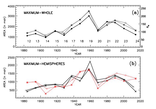
Figure 2.: The values of maxima of Solar Cycles 12 – 24 versus their corresponding epochs. The crosses indicate the values of $A^{*}_{\rm M}$, which correspond to the epochs of $R_{\rm M}$, the open-circles indicate the values of $A_{\rm M}$, which correspond to the epochs of the actual maxima, and the filled-circles indicate the values of $R_{\rm M}$. (a) The dotted curves represent the variations in $A_{\rm M}$ and $A^{*}_{\rm M}$ obtained from the whole sphere sunspot group data (WSGA) and the continuous curve represents the variation in $R_{\rm M}$ (b) The continuous curves represent the variations in $A_{\rm M}$ and $A^{*}_{\rm M}$ obtained from the northern hemisphere data (NSGA), and the dotted curves (red) represent the corresponding variations obtained from the southern-hemisphere data (SSGA), In panel a the Waldmeier numbers of solar cycles are also given.

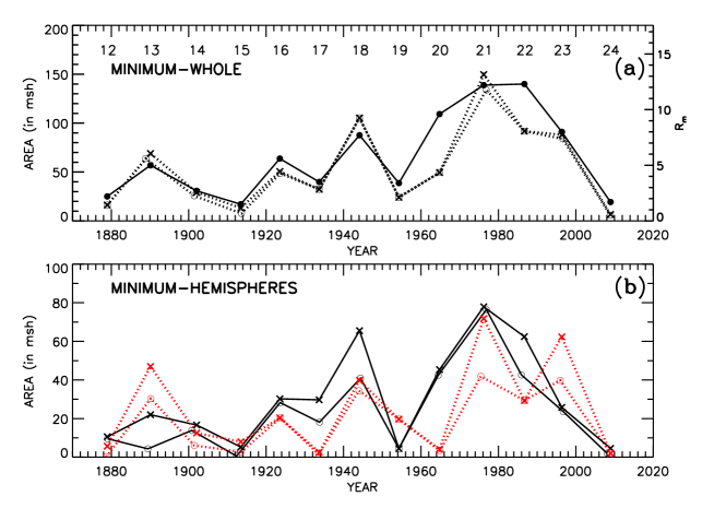
Figure 3.: The values of the minima of the Solar Cycles 12 – 24 versus their corresponding epochs. The crosses indicate the values of $A^{*}_{\rm m}$ that correspond to the epochs of $R_{\rm m}$, the open-circles indicate the values of $A_{\rm m}$ that correspond to the epochs of the actual minima, and the filled-circles indicate the values of $R_{\rm m}$. (a) The dotted curves represent the variations in $A_{\rm m}$ and $A^{*}_{\rm m}$ obtained from the whole-sphere sunspot-group data (WSGA) and the continuous curve represents the variation in $R_{\rm m}$, and (b) The continuous curves represent the variations in $A_{\rm m}$ and $A^{*}_{\rm m}$ obtained from the northern hemisphere data (NSGA) and the dotted curves (red) represent the corresponding variations obtained from the southern hemisphere data (SSGA). In panel a the Waldmeier numbers of solar cycles are also given.

Figure 4.: The cycle-to-cycle variations in the North–South asymmetry (a) in the maximum and (b) in the minimum of the Solar Cycles 12 – 24. The open-circle-dotted curves represent the North–South asymmetry in $A^{*}_{\rm M}$ and $A^{*}_{\rm m}$ and the filled circle-continuous curves represent the North-South asymmetry in $A_{\rm M}$ and $A_{\rm m}$. The positive and negative values imply the North dominance and the South dominance, respectively.

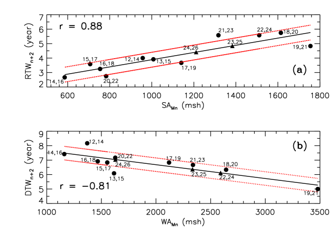
Figure 5.: Scatter plots of (a) $SA_{{\rm M}_{n}}$: the maximum [$A_{\rm M}$] of Solar Cycle $n$ of the area of sunspot groups in southern hemisphere (SSGA) versus $RTW_{n+2}$: the rise time (RT) of Cycle $n+2$ of the area of sunspot groups in whole sphere (WSGA), (b) $WA_{{\rm M}_{n}}$: $A_{\rm M}$ of Solar Cycle $n$ of the area of sunspot groups in whole hemisphere (WSGA) versus $DTW_{n+2}$: the decline time (DT) of Cycle $n+2$ of the area of sunspot groups in whole sphere (WSGA). The continuous line represents the best linear least-square fit and the dotted lines (red) are drawn at one-rmsd (root-mean-square deviation). The values of the correlation coefficient [$r$] are also given. The filled triangles represent the predicted values of the Cycles 25 and 26 in the case of (a) and the Cycles 24, 25, and 26 in the case of (b).

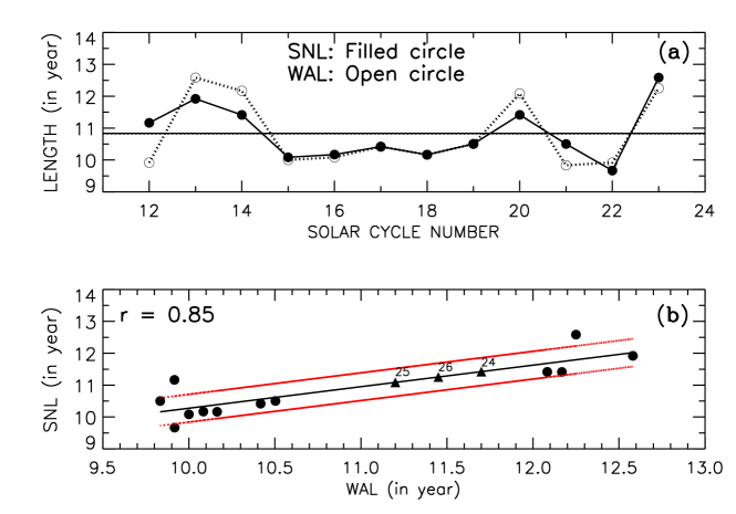
Figure 6.: (a) NSL and WSL, $i.e.$ lengths of ISSN and WSGA cycles, respectively, versus solar-cycle number. (b) Scatter plot of NSL versus WAL. The continuous line represents the best linear least-square fit and the dotted lines (red) are drawn at one-rmsd. The value of $r$ is also given. The filled triangles represent the predicted values of the cycles 24, 25, and 26.

3.2 Prediction of Lengths of Upcoming Solar Cycles

Using the values given in Tables 2 and 3 we determined correlations among the several parameters of solar cycles of different indices. However, only the relations described below are found to be reasonably statistically significant.

Figure 5(a) shows the relationship between the maximum [$A_{\rm M}$] of the SSGA Cycle $n$ (namely $SA_{{\rm M}_{n}}$) and the rise time (RT) of the WSGA Cycle $n+2$ (namely $RTW_{n+2}$). Figure 5(b) shows the relationship between the maximum [$A_{\rm M}$] of the WSGA Cycle $n$ (namely $WA_{{\rm M}_{n}}$) and the decline-time (DT) of the WSGA Cycle $n+2$ (namely $DTW_{n+2}$). We obtained the following linear relations:

$$RTW_{n+2}=(0.0025\pm 0.00045)SA_{{\rm M}_{n}}+1.39\pm 0.53$$

and

$$DTW_{n+2}=(-0.00096\pm 0.00024)WA_{{\rm M}_{n}}+8.6\pm 0.50.$$

The fit of Equation 1 to the data is good. The slope is 5.55 times greater than the corresponding standard deviation and except for the two data points (19, 20) and (21, 23), most of the remaining nine data points are within or very close to the one-root-mean-square deviation ($rmsd=0.51$). The corresponding correlation coefficient $r=0.88$ is statistically significant at the 99.9 % confidence level (Student’s $t=5.5$, which is much higher than the value 4.78 $t$-significance at the 0.1 % level, $P<0.001$, for nine degrees of freedom) and $\chi^{2}=2.29$ is much lower than the value 18.307 $\chi^{2}$ significant on 5% level, $P=0.05$, for ten degrees of freedom. (Note: we have also obtained a positive correlation between $WA_{{\rm M}_{n}}$ and $RTW_{n+2}$, but it is found considerably smaller than that of $SA_{{\rm M}_{n}}$ and $RTW_{n+2}$.)

The fit of Equation 2 to the data is also reasonably good (slightly weaker than that of Equation 1). The slope is four times greater than the corresponding standard deviation and except the two data points (12, 14) and (13, 15), most of the remaining eight data points are within or vary close to the one-rmsd level. The corresponding correlation coefficient $r=-0.81$ is statistically significant at the 99 % confidence level ($t=3.9$, which is slightly higher than the value 3.36 $t$-significant at the 1 % level, $P=0.01$, for 8 degrees of freedom) and $\chi^{2}=3.1$ is much lower than the value 16.919 $\chi^{2}$-significant 5 % level, $P=0.05$, for 9 degrees of freedom.

By substituting the values 1383.22 msh and 1211.0 msh of $SA_{{\rm M}_{n}}$ of the Cycles 23 and 24 in Equation 1 we obtained the values $4.84\pm 0.51$ years and $4.41\pm 0.51$ years for $RTW_{n+2}$, $i.e.$ the rise times of the WSGA Cycles 25 and 26, respectively. By substituting the values 2591.13 msh, 2334.05 msh, and 1628.64 msh of $WA_{{\rm M}_{n}}$ of the WSGA Cycles 22, 23, and 24 in Equation 2 we obtained the values $6.12\pm 0.47$ years, $6.36\pm 0.47$ years, and $7.04\pm 0.47$ years of $DTW_{n+2}$, $i.e.$ the decline-times of WSGA Cycles 24, 25, and 26, respectively. All of these predicted values are also shown in Figure 5. The sum of the values of the rise- and the decline-times gives the lengths (the values of L), $11.7\pm 0.15$ years, $11.2\pm 0.2$ years, and $11.45\pm 0.3$ years of the WSGA Cycles 24, 25, and 26 (in the case of the WSGA Cycle 24 the observed value of the rise time given in Table 3 is used). These predicted values of the lengths suggest that $2020.57\pm 0.15$ (July 2020), $2031.77\pm 0.2$ (October 2031), and $2043.22\pm 0.3$ (March 2043) would be the minimum epochs (start dates) of WSGA Cycles 25, 26, and 27, respectively, and the predicted rise times suggest that $2025.41\pm 0.51$ (May 2025) and $2036.18\pm 0.51$ (March 2036) would be the maximum epochs of WSGA Cycles 25 and 26, respectively.

Figure 6(a) shows the variations in the lengths of ISSN cycle (namely SNL) and WSGA cycle (namely WAL). As can be seen in this figure, only in a few places a considerable difference exists between SNL and WAL. However, both SNL and WAL vary almost identically. In an earlier analysis a cosine fit to the data (length values) of ISSN Cycles 6 – 22 has suggested the existence of a eight-cycle periodicity in the length of ISSN cycle (see Figure 5 of jbu05). Obviously, the patterns of the variations in SNL and WAL are consistent with that earlier result. Figure 6(b) shows the relationship between WAL and SNL. There exists a considerable correlation between WAL and SNL ($r=0.85$, the corresponding $P<0.001$). We obtained the following linear relation between WAL and SNL:

$$SNL=(0.675\pm 0.132)WAL+3.52\pm 1.43\quad.$$

The corresponding least-square fit is reasonably good ($\chi^{2}=3.0$ is small, the slope is 5.1 times larger than the corresponding standard deviation). The $rmsd=0.43$ is reasonably small. Except for two data points (that correspond to the Cycles 12 and 23), all of the remaining data points are inside or on the lines of one-rmsd.

By substituting the predicted values of WAL in Equation 3 we obtained the values $11.42\pm 0.43$ years, $11.09\pm 0.43$ years, and $11.25\pm 0.43$ years for the lengths of ISSN Cycles 24, 25, and 26, respectively. This suggests that the minimum epochs (start dates) of ISSN Cycles 25, 26, and 27 would be $2020.38\pm 0.43$ (May 2020), $2031.47\pm 0.43$ (June 2031), and $2042.72\pm 0.43$ (September 2042), respectively. All of these values seem to be slightly less than the the corresponding predicted values of the WSGA Cycles 24, 25, and 26. However, the differences between the predicted values of the ISSN and WSGA cycles are not significant.

When we have used lengths of Cycles 12 – 13 of the revised time series of sunspot numbers (SN) the correlation between the WAL and NAL is found to be 0.86 ($\chi^{2}=2.84$) and $11.4\pm 0.4$ years, $11.07\pm 0.4$ years, and $11.23\pm 0.4$ years are found for the lengths of Cycles 24, 25, and 26, respectively.

dgt08 found that the Waldmeier effect is not present in the cycles of sunspot-group area. Here, we have also found the same. That is, we find that there exists no significant correlation between rise time and amplitude of WSGA, NSGA, and SSGA cycles. Also no significant correlation is found between the rise times of ISSN and area cycles. Hence, here we cannot predict the rise times of the ISSN Cycles 25 and 26 by using the above-predicted rise times of WSGA Cycles 25 and 26.

As per the above prediction, the length of Solar Cycle 25 would be smaller than those of Cycles 24 and 26. Hence, as per the well-known inverse relationship between cycle amplitude and length, the above predicted lengths indicate that Cycle 25 would be stronger than Cycles 24 and 26. This contradicts our prediction (jj15, 2017). However, the variations in solar cycle length and amplitude are not perfectly in phase or anti-phase (hs97). In fact, only a weak correlation exists between length and amplitude of a cycle ($e.g.$ solanki02).

There exits a highly statistically significant inverse relationship between length of a cycle and the amplitude of the following cycle (hath94; solanki02; hath15). As per this relationship the above-predicted lengths of the ISSN-cycles 24, 25, and 26 indicate that Cycle 25 would be stronger than the Cycle 24 (Note: the length, 12.25 year, of Cycle 23 is larger than the predicted length of Cycle 24). Hence, this is also a contradiction to our earlier prediction that Cycle 25 will be weaker than Cycle 24 (jj15, 2017). On the other hand the corresponding correlations of all of the present predictions are not very high.

3.3 Asymmetry at the Epochs of the Actual Maxima and Minima of NSGA- and SSGA-cycles

It should be noted that the epochs of the actual maximum [$A_{\rm M}$], as well as those of the actual minimum [$A_{\rm m}$], of NSGA- and SSGA-cycles are different in many cycles. In Section 3.1 we have shown the asymmetry between the $A_{\rm M}$ of NSGA and $A_{\rm M}$ of SSGA and between the $A_{\rm m}$ of NSGA and $A_{\rm m}$ of SSGA (the filled-circle-continuous curves in Figure 4).

The upper panel of Figure 7 shows the cycle-to-cycle modulation in $A^{*}_{\rm N}$, $i.e.$ the value of NSGA at the epoch of $A_{\rm M}$ of SSGA-cycle, and the modulation in $A^{*}_{\rm S}$, $i.e.$ the value of SSGA at the epoch of $A_{\rm M}$ of NSGA-cycle (the values $A^{*}_{\rm N}$ and $A^{*}_{\rm S}$ are also given in Table 2). In this figure the modulation in $A_{\rm M}$ of NSGA-cycle and that in $A_{\rm M}$ of SSGA-cycle (which are already shown in Figure 2) are also shown for the sake of comparison of these with those of $A^{*}_{\rm N}$ and $A^{*}_{\rm S}$. In the lower panel of Figure 7 the cycle-to-cycle modulation in the asymmetry between the $A_{\rm M}$ of NSGA and $A^{*}_{\rm S}$ and the modulation in the asymmetry between the $A_{\rm M}$ of SSGA and $A^{*}_{\rm N}$ are shown. Figure 8 is same as Figure 7, but for the data at the epochs of actual minima of NSGA- and SSGA-cycles.

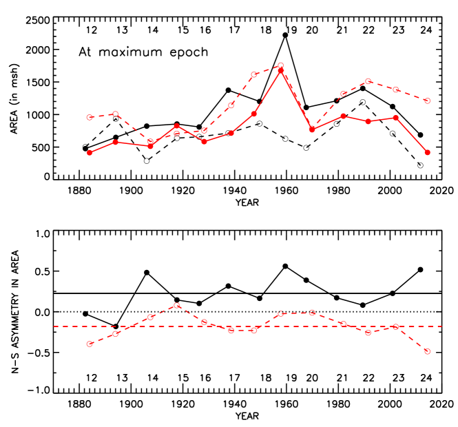
Figure 7.: Upper panel: The maximum [$A_{\rm M}$] value of NSGA (SSGA) cycle (also shown in Figure 2) and the value of $A^{*}_{\rm S}$ ($A^{*}_{\rm N}$) of SSGA (NSGA) at the epoch of the maximum of NSGA (SSGA) cycle (which are also given Table 2) versus time ($i.e.$ epoch of maximum). The filled circle-continuous curves represent the modulations in $A_{\rm M}$ of NSGA-cycle and $A^{*}_{\rm N}$, $i.e.$ the value of NSGA at the epoch of the maximum of the SSGA-cycle. The open-circle-dashed curves represent the variations in $A_{\rm M}$ of SSGA-cycle and $A^{*}_{\rm S}$, $i.e.$ the value of SSGA at the epoch of the maximum of the NSGA-cycle. The corresponding quantities at the epochs of maxima of NSGA- and SSGA-cycles are shown by black and red colors, respectively. Lower panel: The black filled-circle-continuous curve and the red open-circle-dashed curve represent the variations of North–South asymmetry in the corresponding quantities at the epochs of the maxima of NSGA- and SSGA-cycles, respectively. The positive and negative values imply the North dominance and the South dominance, respectively.

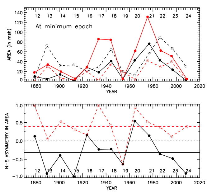
Figure 8.: Upper panel: The minmum [$A_{\rm m}$] value of NSGA (SSGA) cycle (also shown in Figure 3) and the value of $A^{*}_{\rm S}$ ($A^{*}_{\rm N}$) of SSGA (NSGA) at the epoch of the minimum of NSGA (SSGA) cycle (which are also given in Table 2) versus time ($i.e.$ epoch of minimum). The filled circle-continuous curves represent the variations in the minimum of NSGA-cycle [$A_{\rm m}$] and $A^{*}_{\rm N}$, $i.e.$ the value of NSGA at the epoch of the minimum of SSGA-cycle. The open-circle-dashed curves represent the variations in the $A_{\rm m}$ of SSGA-cycle and $A^{*}_{\rm S}$, $i.e.$ the value of SSGA at the epoch of the minimum of NSGA-cycle. The quantities at the epochs of minima of NSGA- and SSGA-cycles are shown by black and red colors, respectively. Lower panel: The black filled-circle-continuous curve and the red open-circle-dashed curve represent the variations of North–South asymmetry in the corresponding aforementioned quantities at the epochs of the minima of NSGA- and SSGA-cycles, respectively. The positive and negative values imply the North dominance and the South dominance, respectively.

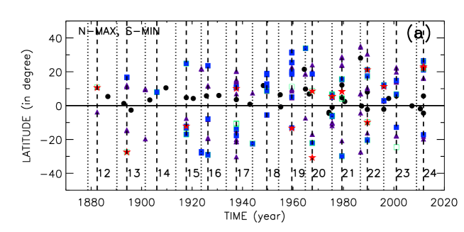
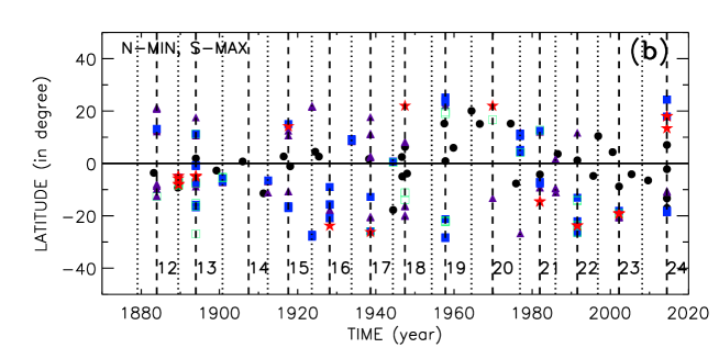
Figure 9.: Latitude–time distributions of sunspot groups: (a) the latitude distributions of sunspot groups at the epochs of $A_{\rm M}$ of NSGA-cycles and at the epochs of $A_{\rm m}$ of SSGA-cycles, and (b) the latitude distributions of sunspot groups at the epochs of $A_{\rm M}$ of SSGA-cycles and at the epochs of $A_{\rm m}$ of NSGA-cycles. The sunspot groups having areas 0 – 100 msh, 100 – 200 msh, 200 – 300 msh, 300 – 400 msh, and 400 – 500 msh are indicated by the filled-circle (black), filled-triangle (light-blue), filled-square (blue), open-squre (green), and filled-star (red), respectively. The dotted- and dashed-vertical lines are drawn at the epochs of the minimum [$A_{\rm m}$] and maximum [$A_{\rm M}$], respectively. Waldmeier cycle numbers are shown near the epochs of maxima of the cycles. (Note: here the time intervals $ME$ to $ME+0.01$ and $me$ to $me+0.1$ are used, where $ME$ and $me$ are the epochs of maximum and minimum, respectively.)

As can be seen in the upper panel of Figure 7, except for Cycles 12 and 13, for all of the other cycles $A_{\rm M}$ of NSGA-cycle is larger than $A^{*}_{\rm S}$ (see black curves in the upper panel, also see Table 2). Obviously, the mean value of the asymmetry between these quantities suggests that the activity is dominant in the northern hemisphere (see the black curve in the lower panel). The pattern of the variation in the asymmetry suggests that there exists an $\approx$55-year periodicity (there are large positive values at Cycles 14, 19, and 24). The pattern of a 130 – 140-year cycle that is seen in Figure 4(a) is not clear here. Except at the Cycles 14, 15, and 20, for the remaining cycles $A_{\rm M}$ of SSGA-cycle is considerably larger than $A^{*}_{\rm N}$ (see the red curves in the upper panel). (For Cycle 15 the $A_{\rm M}$ of the SSGA-cycle is slightly smaller than $A^{*}_{\rm N}$.) Obviously, the mean value of the corresponding asymmetry suggests that the activity is dominant in the southern hemisphere (see the red curve in lower panel). There are patterns of an $\approx$55-year cycle and there is also a trend of a 130 – 140-year periodicity (the values of the asymmetry has a large negative values at Cycles 12 and 24.)

As can be seen in the upper panel of Figure 8, the patterns of variations in all of the quantities that are shown in it are similar and there are patterns of 44 – 66 years periodicity in each quantity. Except for Cycle 19, for the remaining cycles $A_{\rm m}$ of SSGA-cycle is smaller than $A^{*}_{\rm N}$ (see the red curves in the upper panel, also see Table 2). For Cycles 12 and 16 and particularly for Cycles 20 and 21 the $A_{\rm m}$ of NSGA-cycle is larger than the corresponding $A^{*}_{\rm S}$ (see the black curves in the upper panel). For all of the remaining cycles $A_{\rm m}$ of the NSGA-cycle is smaller than $A^{*}_{\rm S}$. There exists a 44 – 66 year periodicity in both the asymmetry between the $A_{\rm m}$ of NSGA-cycle and the corresponding $A^{*}_{\rm S}$ and that between the $A_{\rm m}$ of SSGA-cycle and the corresponding $A^{*}_{\rm N}$ (see the lower panel of Figure 8)

Overall, the above results suggest that a 44 – 66-year periodicity is present in the North–South asymmetry of activity at the epochs of both minima and maxima of NSGA- and SSGA-cycles. A long (130 – 140 years) periodicity may exist in the North–South asymmetry at the maxima of SSGA-cycles, but as already mentioned in Section 3.1 the 143 years of data used here are inadequate to determine the precise value of this periodicity.

During the Maunder Minimum (1645 – 1715) sunspot activity was not completely absent. That is, during the late Maunder Minimum activity was present in the low latitudes (between $0^{\circ}$ and $-20^{\circ}$) of the southern hemisphere (see Figure 1(a) of soko94). Figure 9(a) shows the latitude distributions (tentative) of sunspot groups at the epochs of maxima of NSGA-cycles and at the epochs of minima of SSGA-cycles. At these epochs the activity is more in the northern hemisphere (also see Figures 7 and 8). Figure 9(b) is same as Figure 9(a) but for the latitude distributions of sunspot groups at the epochs of maxima of SSGA-cycles and at the epochs of minima of NSGA-cycles. At these epochs, except in a few cycles (Cycles 19, and 20), the activity is greater in the southern hemisphere (also see Figures 7 and 8). (Note: The epochs of maxima and the minima were obtained from the 13-month smoothed data. In Figure 9 we have used the daily data very close to these epochs of maxima and minima.) The pattern of activity (in Cycles 12 – 18 and Cycles 21 – 23) shown in Figure 9(b) is qualitatively similar to the pattern of activity during the late Maunder Minimum (1670 – 1715, in about four cycles). Therefore, it seems that during the late Maunder Minimum activity was absent around the epochs of the maxima of NSGA-cycles and the minima of SSGA-cycles, and some activity was present at the epochs of the maxima of some SSGA-cycles and the minima of some NSGA-cycles. We think that during the late Maunder Minimum, because of unique alignments of the giant planets (jj05) there could be a large combined affect of the Sun’s rotation and the inclination of the Sun’s Equator to the Ecliptic causing equatorial crossing of a large amount of the magnetic flux of the southern hemisphere. This canceled the flux of northern hemisphere. The cancellation of flux might have taken place in the deeper layers of the Sun’s convection zone.

4 Conclusions and Discussion

The North–South asymmetry in solar activity may have some important implications for the solar dynamo mechanism. We analyzed the combined GPR and DPD daily sunspot group data during the period 1874 – 2017 and studied the North–South asymmetry in the maxima and minima of Solar Cycles 12 – 24. We derived the time-series of the 13-month smoothed monthly mean corrected whole-spot areas of the sunspot groups in the Sun’s whole sphere (WSGA), northern hemisphere (NSGA), and southern hemisphere (SSGA). From these smoothed time series we obtained the values of the maxima and minima, and the corresponding epochs, of the WSGA, NSGA, and SSGA Cycles 12 – 24. We find that a 44 – 66-year periodicity exists in the North–South asymmetry of minimum. A long periodicity (130 – 140 years) may exit in the asymmetry of maximum. A statistically significant correlation exists between the maximum of SSGA Cycle $n$ and the rise time of WSGA Cycle $n+2$. A reasonably significant correlation also exists between the maximum of WSGA Cycle $n$ and the decline time of WSGA Cycle $n+2$. Using these relations we obtained the values $11.70\pm 0.15$ years, $11.2\pm 0.2$ years, and $11.45\pm 0.3$ years for the lengths of WSGA Cycles 24, 25, and 26, respectively, and hence, $2020.57\pm 0.15$ (July 2020), $2031.77\pm 0.2$ (October 2031), and $2043.22\pm 0.3$ (March 2043) for the minimum epochs (start dates) of WSGA Cycles 25, 26, and 27, respectively. We also obtained $2025.41\pm 0.51$ (May 2025) and $2036.18\pm 0.51$ (March 2036) for the maximum epochs of WSGA Cycles 25 and 26, respectively. Our analysis also suggests that the lengths and the starting times of ISSN Cycles 24, 25, and 26 would be almost the same as the corresponding WSGA-cycles. It seems during the late Maunder Minimum sunspot activity was absent around the epochs of the maxima of NSGA-cycles and the minima of SSGA-cycles, and some activity was present at the epochs of the maxima of some SSGA-cycles and the minima of some NSGA-cycles.

The ratio of the number of large sunspot groups to the number of small sunspot groups is generally smaller in the minimum than in the maximum of a solar cycle. That is, the epochs of the minima and maxima of solar cycles comprise relatively small and large numbers of large sunspot groups, respectively. The magnetic structures of large and small sunspot groups are rooted at relatively deep and shallow layers of the solar convection zone (jg97b; kmh02; siva03). Hence, the long-term periodicities of the North–South asymmetry in the maxima and minima of solar cycles might originate at relatively deep and shallow layers of the solar convection zone, respectively. Therefore, there could be differences in the long-term variations of solar maximum and minimum and in their North–South asymmetry. However, the physical reason for the existence of the 130 – 140-year and 44 – 66-year periodicities in the North–South asymmetry of solar activity is not clear. In fact, these periodicities seem to be a common features of many solar and solar-related phenomena, but the physical processes responsible for these also are not clear yet ($e.g.$ tan11; gao16; komit16, and references therein). On the other hand there could be a connection between solar variability (both long- and short-term) and planetary configurations (juc03; jj05, abreu12; cc12; wil13; chow16; stef16, and references therein).

In our earlier studies the amount of activity in the northern hemisphere around minimum and mainly in the southern hemisphere during the declining phase of the Solar Cycle $n$ correlated with the amplitude of Cycle $n+1$ (jj07; 2008; 2015). Here, we find that the amplitude of the Cycle $n$ correlate with the rise time, and anticorrelate with the declining-time, of Cycle $n+2$. Altogether these results suggest that solar dynamo carries memory over at least three solar cycles. It is consistent with the kind of flux transport dynamo model in which a long magnetic memory is an important criteria (dg06). A low amplitude predicted for Cycle 25 in jj15 and the maximum epoch of WSGA Cycle 25 predicted here qualitatively match the recent predictions of the amplitude and maximum epoch of this solar cycle by an advanced flux transport model based on the polar fields at cycle minimum (lh18). However, the predictions based on the polar fields at cycle minimum could be uncertain because it was unclear exactly when these polar-field measurements should be taken (sval05) and Cycle 24 has not yet ended. The aforementioned relationships of the amplitude of WSGA-Cycle $n$ with rise and decline times of Solar Cycle $n+2$ imply that an odd (even) cycle have a connection with its previous odd (even) cycle. As in Javaraiah (2007, 2008, 2015), here also we would like to suggest that the aforementioned relationships may be also related to the changes in the polarities of the Sun’s magnetic fields and both meridional and down flows have roles in the magnetic-flux transport. Polar fields change sign about one year after the maximum of a cycle takes place. The polarities of the fields at the maximum epoch of Cycle $n$, the declining phase of Cycle $n+1$, and the rising phase of Cycle $n+2$ differ from those of the fields at the declining phase of Cycle $n$, the rising phase of Cycle $n+1$, and the declining phase of Cycle $n+2$. Therefore, a physical reason behind the Equation 1 may be that a large southern-hemisphere flux transported from the maximum of a large Cycle $n$ may cancel a relatively large amount of northern-hemisphere flux in the rising phase (including minimum epoch) of Cycle $n+2$ ($i.e.$ it decreases the rate of flux emergence) causing an increase in the rise time of Cycle $n+2$. A physical reason behind Equation 2 may be that a large flux transported from the maximum of a large Cycle $n$ may cancel a relatively large amount of flux in the declining phase of Cycle $n+2$ ($i.e.$ it enhances the rate of flux decay) causing a decrease in decline time of Cycle $n+2$.

As per the aforementioned physical interpretation of Equation 1 even- and odd-numbered solar cycles could be arranged separately according to their strengths as follows: $12>14<16<18>20<22>24<26?$ and $13>15<17<19>21>23<25?$ (if Cycle 23 is considered as a reasonably small odd-numbered cycle). However, we think that the relationships (between two consecutive sunspot cycles) that yielded a low amplitude for Cycle 25 in an our earlier analysis (jj15) are much stronger than the relationships (between alternate cycles) found here. In addition, at least at the time of a steep decrease in the orbital angular momentum of the Sun may have an effect on the Sun’s rotation and hence, the corresponding change in the Sun’s spin-rate may be responsible for a grand minimum type of low activity (jj05). The next unique alignments of the giant planets and hence, the steep decrease in the Sun’s orbital angular momentum will be taking place in 2030 (see jj05). Cycles 25 and 26 will be taking place in the vicinity of 2030 and both might be weaker than Cycle 24, as predicted by jj17. On the other hand, the exact physical reason behind the aforementioned all relations needs to be established.

5 Acknowledgments

The author thanks the anonymous referee for useful comments and suggestions. The author acknowledges the work of all the people contribute and maintain the GPR and DPD Sunspot databases. The sunspot-number data are provided by WDC-SILSO, Royal Observatory of Belgium, Brussels.

6 Disclosure of Potential Conflicts of Interest

The author declares that he has no conflicts of interest.

References

- Abreu et al. (2012) Abreu, J.A., Beer, J., Ferriz-Mas, A., McCracken K.G., Steinhilber, F.: 2012, Astron. Astrophys. 548, A88. DOI: 10.1051/0004-6361/201219997
- Belucz and Dikpati (2013) Belucz, B., Dikpati, M.: 2013, Astrophys. J. 779, 4. DOI: 10.1088/0004-1075637X/779/1/4
- Carbonell et al. (1993) Carbonell, M., Oliver, R., Ballester, J.L.: 1993, Astron. Astrophys. 274, 497.
- Chowdhury et al. (2013) Chowdhury, P., Choudhary, D. P., Gosain, S.: 2013, Astrophys. J. 768, 188. DOI: 10.1088.004-637X/768/2/188
- Chowdhury et al. (2016) Chowdhury, P., Gokhale, M.H., Singh, J., Moon, Y.-J.: 2016, Astrophys. Space Sci., 361, 54. DOI: 10.1007/s10509-015-2641-8
- Cionco and Compagnucci (2012) Cionco, R.G., Compagnucci, R.H.: 2012, Adv. Space Res. 50, 1434. DOI: 10.1016/j.asr.2012.07.013
- DeRosa, Brun, and Hoeksema (2012) DeRosa, M.L., Brun, A.S., Hoeksema, J.T.: 2012, Astrophys. J. 757, 96. DOI: 10.1088/0004-637X/757/1/96
- Dikpati and Gilman (2006) Dikpati, M., Gilman, P.A.: 2006, Astrophys. J. 649, 498. DOI: 10.1086/506314
- Dikpati, Gilman, and de Toma (2008) Dikpati, M., Gilman, P. A., de Toma, G.: 2008, Astrophys. J. Lett. 673, L99. DOI: 10.1086/527360
- Foukal (1972) Foukal, P.V.: 1972, Astrophys. J. 173, 439. DOI: 10.1086/151435
- Gao (2016) Gao, P.X.: 2016, Astrophys. J., 830, 140. DOI: 10.3847/0004-637X/830/2/140
- Gilman and Foukal (1979) Gilman, P.A., Foukal, P.V.: 1979, Astrophys. J. 229, 1179. DOI: 10.1086/157052
- Gnevyshev (1963) Gnevyshev, M.N., 1963, Sov. Astron. 7, 311.
- Győri, Baranyi, and Ludmány (2010) Győri, L., Baranyi, T., Ludmány, A.: 2010, in Proc. Intern. Astron. Union 6, Sympo. S273, 403. DOI: 10.1017/s174392131101564X
- Hathaway, Wilson, and Reichmann (1994) Hathaway, D.H., Wilson, R.M. and Reichmann, E.J.: 1994, Solar Phys. 151, 177. DOI: 10.1007/BF00654090
- Hathaway (2015) Hathaway, D.H.: 2015, Liv. Rev. Solar. Phys. 12(4), 1. DOI: 10.1007/1rsp-2015-4
- Hiremath (2002) Hiremath, K.M.: 2002, Astron. Astrophys. 386, 674. DOI: 10.10.1051/0004-6361:20020276
- Howard (1996) Howard, R.F.: 1996, Ann. Rev. Astron. Astrophys. 34, 75. DOI: 10.1146/annurev.astro.34.1.75
- Hoyt and Schatten (1997) Hoyt, D.V., Schatten, K.H.: 1997, The Role of the Sun in Climate Change, Oxford University Press, New York. DOI: 10.1111/j.1365-2966.2005.09403.x
- Javaraiah (2005) Javaraiah, J.: 2005, Mon. Not. Roy. Astron. Soc. 362, 1311. DOI: 10.1111/j.1365-2966.2005.09403.x
- Javaraiah (2007) Javaraiah, J.: 2007, Mon. Not. Roy. Astron. Soc. 377, L34. DOI: 10.1111/j.1745-3933.2007.00298.x
- Javaraiah (2008) Javaraiah, J.: 2008, Solar Phys. 252, 419. DOI: 10.1007/s11207-008-9269-6
- Javaraiah (2012) Javaraiah, J.: 2012, Solar Phys. 281, 827. DOI: 10.1007/s11207-012-0106-6
- Javaraiah (2015) Javaraiah, J.: 2015, New Astron. 34, 54. DOI: 10.1016/j.newast.2014.04.001
- Javaraiah (2016) Javaraiah, J.: 2016, Astrophys. Space Sci., 361, 208. DOI: 10.1007/s10509-016-2797-x
- Javaraiah (2017) Javaraiah, J.: 2017 Solar Phys. 292, 172. DOI: 10.1007/s11207-017-1197-x
- Javaraiah and Gokhale (1997a) Javaraiah, J., Gokhale, M.H., 1997a, Solar. Phys. 170, 389. DOI: 10.1023/A:1004928020737
- Javaraiah and Gokhale (1997b) Javaraiah, J., Gokhale, M.H.: 1997b, Astron. Astrophys. 327, 795.
- Javaraiah, Bertello, and Ulrich (2005) Javaraiah, J., Bertello, L., Ulrich, R.K.: 2005, Solar Phys. 232, 25. DOI: 10.1007/s11207-005-8776-y
- Juckett (2003) Juckett, D.A.: 2003, Astron. Astrophys. 399, 731. DOI: 10.1051/0004-6361:20021923
- Kane (2007) Kane, R.P.: 2007, Solar Phys. 243, 205. DOI: 10.1007/s11207-007-0475-4
- Komitov et al. (2016) Komitov, B., Sello, S., Duchlev, P., Dechev, M., Penev, K., Koleva, K.: 2016, Bulg. Astronomic. J. 25, 78.
- Mandal and Banerjee (2016) Mandal, S., Banerjee, D.: 2016, Astrophys. J. Lett. 830, L33. DOI: 10.3847/2041-8205/830/2/L33
- Norton and Gallagher (2010) Norton, A.A., Gallagher, J. C.: 2010, Solar Phys. 261, 193. DOI: 10.1007/s11207-009-9479-6
- Obridko and Shelting (2008) Obridko, V.N., Shelting, B.D.: 2008, Solar Phys. 248, 191. DOI: 10.1007/s11207-008-9138-3
- Pesnell (2008) Pesnell, W.D.: 2008, Solar Phys. 252, 209. DOI: 10.1007/s11207-008-9252-2
- Pesnell and Schatten (2018) Pesnell, W.D., Schatten, K.H.:: 2018, Solar Phys. 293, 112. DOI: 10.1007/s11207-018-1330-5
- Ramesh and Rohini (2008) Ramesh, K.B., Rohini, V.S.: 2008, Astrophys. J. Lett. 686, L41. DOI: 10.1086/592774
- Ravindra and Javaraiah (2015) Ravindra, B., Javaraiah, J.: 2015, New Astron. 39, 55. DOI: 10.1016/j.newast.2015.03.004
- Sarp et al. (2018) Sarp, V., Kilcik, A., Yarchyshyan, V., Rozelot, J.P., Ozguc, A.: 2018, Mon. Not. Roy. Astron. Soc. 481, 2981. DOI: 10.1093/mnras/sty2470
- Shetye, Tripathi, and Dikpati (2015) Shetye, J., Tripathi, D., Dikpati, M.: 2015, Astrophys. J. 799, 220. DOI: 10.1088/0004-637X/799/2/220
- Sivaraman et al. (2003) Sivaraman, K.R., Sivaraman, H., Gupta, S.S., Howard, R.: 2003, Solar Phys. 214, 65. DOI: 10.1086/148143/A:1024075100667
- Sokoloff and Nesme-Ribes (1994) Sokoloff, D., Nesme-Ribes, E.: 1994, Astron. Astrophys. 288, 293.
- Solanki et al. (2002) Solanki, S.K., Krivova, N.A., Schüssler, M., Fligge, M.: 2002, Astron. Astrophys. 396, 1029. DOI: 10.1051/0004-6361:20021436
- Stefani et al. (2016) Stefani, F, Giesecke, A., Weber, N., Weier, T.: 2016, Solar Phys. 291, 2197. DOI: 10.1007/s11207-016-0968-0
- Svalgaard et al. (2005) Svalgaard, L., Cliver, E.W., Kamide, Y.: 2005, Geophys. Res. Lett. 32, L01104. DOI: 10.1029/2004GL021664
- Tan (2011) Tan, B.: 2011, Astrophys. Space Sci., 332, 65. DOI: 10.1007/s10509-010-0496-6
- Verma (1993) Verma, V.K.: 1993, Astrophys. J. 403, 797. DOI: 10.1086/172250
- Upton and Hathaway (2018) Upton, L.A., Hathaway, D.H.: 2018, Geophys. Res. Lett. 45, 8091. DOI: 10.1029/2018GL078387
- Vizoso and Ballester (1990) Vizoso, G., Ballester, J.L.: 1990, Astron. Astrophys. 229, 540.
- Waldmeier (1935) Waldmeier, M.: 1935, Astron. Mitt. Zurich 14(133), 105.
- Waldmeier (1939) Waldmeier, M.: 1939, Astron. Mitt. Zurich 14(138), 470.
- Wilson (2013) Wilson, I.R.G.: 2013, Pattern Recog. Phys. 1, 147. DOI: 10.5194/prp-1-147-2013