Radar-only ego-motion estimation in difficult settings via graph matching
Abstract
Radar detects stable, long-range objects under variable weather and lighting conditions, making it a reliable and versatile sensor well suited for ego-motion estimation. In this work, we propose a radar-only odometry pipeline that is highly robust to radar artifacts (e.g., speckle noise and false positives) and requires only one input parameter. We demonstrate its ability to adapt across diverse settings, from urban UK to off-road Iceland, achieving a scan matching accuracy of approximately 5.20 cm and 0.0929 deg when using GPS as ground truth (compared to visual odometry’s 5.77 cm and 0.1032 deg). We present algorithms for keypoint extraction and data association, framing the latter as a graph matching optimization problem, and provide an in-depth system analysis.
I Introduction
Despite the rapid expansion and advancement of research into sensor systems for mobile autonomy, those used for intelligent transportation typically feature the same suite: vision, lidar, GPS, and proprioceptive sensors. Recent interest in radar for mobile autonomy [1, 2] has uncovered its potential as a highly robust, multipurpose sensor. Unlike vision and lidar systems, it is resilient to variable lighting and weather, and, unlike GPS, it functions both indoors and outdoors. Radar is reliable at short and long ranges, and it is becoming increasingly more compact and affordable. In addition to its practical benefits, radar returns are simultaneously data-efficient and information-rich: radar can observe multiple objects per transmission and detect their locations, velocities, and cross-section characteristics.
As a result, radar is a highly versatile sensor that can withstand adverse conditions. Its ability to detect stable, long-range features makes it particularly suitable for odometry and localization. In this paper, we build on our previous work [2], in which we demonstrate precise ego-motion estimation using only a millimeter-wave (MMW) frequency-modulated continuous-wave (FMCW) scanning radar. As shown in [2], our system performs comparably to state-of-the-art visual odometry (VO) and GPS. Even under conditions that cause other sensors to fail, radar odometry (RO) is robust.
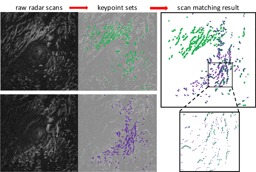
Common approaches to odometry for rangefinders have several key drawbacks, such as sensitivity to noise, reliance on other sensors, requiring a priori knowledge, and utilizing restrictive models. In contrast, our radar-only system achieves precise odometry without model-reliant motion filters, outlier detection, or map creation. At its core is a geometrically-based, non-iterative scan matching algorithm that is displacement-independent and approximately optimizes a global objective function. Consequently, our pipeline works without a prior on the temporal or spatial relationship between keypoint sets and can handle significant measurement noise and missing detections, as shown in Fig. 1.

In this paper, we present a revised system that features the same advantages enumerated above with several major improvements to [2]. Specifically, our main contributions are:
-
•
A new gradient-based, one-parameter keypoint extraction algorithm that functions well in diverse settings.
-
•
More efficient and robust data association.
-
•
Successful real-time odometry in varied and challenging settings (e.g., off-road path in Iceland boulder field).
-
•
In-depth theoretical analysis on system complexity and estimation uncertainty.
Following a literature review in Section II, we present and analyze our pipeline in Sections III and IV. We provide experimental results and conclude in Sections V and VI. Both our works are presented and analyzed in detail in [3].
II Related works
While visual [4, 5], lidar [6, 7], and wheel [8] odometry are well studied, radar odometry remains challenging. Due to its wide spreadbeam and long range, radar has lower resolution than lidar and is highly susceptible to interference from clutter, which generates speckle noise. Radar scans also contain false positives from multipath reflections and receiver saturation. As a result, radar odometry must be robust to measurement noise and false detections, and it must demonstrate high precision despite low-resolution data and slow update speeds. Odometry methods for radar can be categorized as indirect or direct. Indirect methods first extract salient keypoints, then associate those that correspond to the same location. Direct methods [9, 10, 11], which forego keypoint extraction and operate on minimally pre-processed sensor outputs, are discussed in [3, 2] and not in this paper. All methods assume the majority of observed objects are static.
The first step of indirect methods is keypoint extraction, for which the most popular approach is constant false-alarm rate (CFAR) detection [12], which distinguishes peaks from noise using sliding-window thresholding. CFAR and its variants generally require at least three tunable parameters, which are based on assumed noise characteristics and do not behave consistently across datasets (see [2] for comparison). Some works leverage the knowledge that coherent structures make good keypoints by clustering or detecting the edges of bright regions in scans [13]. Others elect to represent the surroundings using predetermined geometric primitives [14] or models, like the normal distribution transform (NDT) [15]. Vision-inspired works treat radar scans as images and extract features, like SIFT and FAST [16].
These keypoints must then undergo data association, also known as scan matching [1, 14] in robotics. The most common technique is iterative closest point (ICP) [17], which iteratively matches points using naive methods until the alignment between keypoint sets is sufficiently close [14, 18]. ICP relies on a good estimate of the relative displacement (i.e., motion prior) between scans. Other data association techniques search for motion parameters that optimize some objective function, like maximizing similarity (e.g., overlap of Gaussian distributions for NDT [19]) or minimizing distance (e.g., cluster edge difference [9]) between keypoint sets. Two further examples of objective functions characterize map quality [20] and radar scan distortion [21] in terms of motion. Feature-based approaches associate keypoints using descriptors, like BASD [22] and SURF [16].
Many of the methods discussed do not generalize well due to the high levels of noise in radar scans. Adequate performance often requires fine tuning, a priori knowledge, restrictive assumptions, or outlier detection. Several of the works rely heavily on other sensors for robustness, which compromises performance under conditions that cause these sensors to fail, or use simultaneous localization and mapping (SLAM), which is accompanied by overhead costs and model-reliant motion filters [23, 16].
We utilize an indirect method to explicitly select salient information from noisy artifacts. We present two algorithms that improve on our previous work [2]. The new pipeline is more efficient and easily adaptable across diverse settings. Accordingly, our keypoint extraction algorithm returns interpretable features with minimal redundancy, only one input parameter, and no assumptions about the scene structure or noise. Our data association algorithm does not need a motion prior or parameter tuning, and it is robust to large amounts of noise and false detections. An in-depth literature review and description of our contributions can be found in [3].
III Radar-only ego-motion estimation
III-A FMCW scanning radar
FMCW radar, which is becoming more compact, safe, and affordable than alternative radars, collects long-range measurements with high accuracy and remains resilient under variable lighting and weather [3]. Scanning radar, as shown in Fig. 2, sequentially observes narrow angular regions as it rotates, allowing it to locate an object that falls inside the transmitted beam by its range and azimuth. Received power depends on object reflectivity, surface area, orientation, and material. A wide spreadbeam in elevation and long wavelength allow multiple objects to be detected per transmission.
For each azimuth, radar outputs a one-dimensional signal, termed the power-range spectrum, which encodes the power reflected by the scatterers within the beam at each range. After a full rotation, radar returns a two-dimensional scan, as shown in Fig. 2. Radar scans are both information-rich and data-efficient, but they contain several unwanted artifacts visible in Fig. 2, including noise and false detections [3]. Another consideration of radar is its lower resolution and slower measurement update speeds compared to lidar.
III-B Keypoint extraction
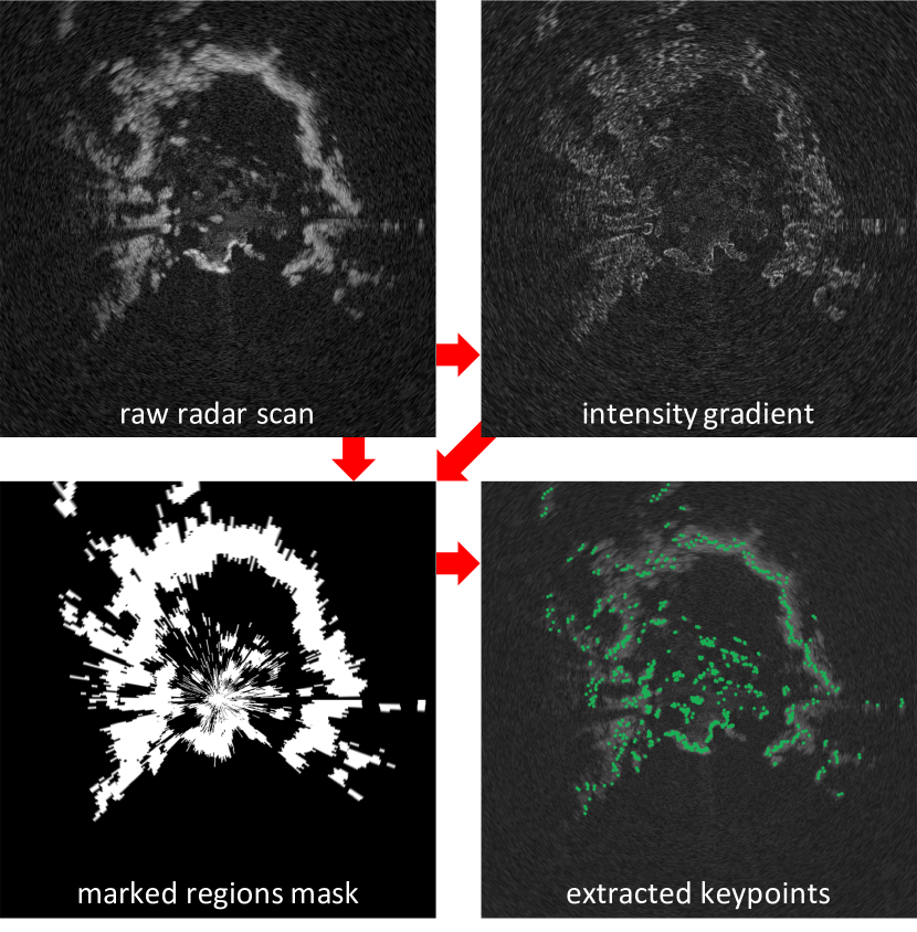
In this section, we present a keypoint extraction algorithm that is designed to:
-
•
Return interpretable and meaningful keypoints.
-
•
Be straightforward to use and require only one input parameter specifying the maximum number of keypoints.
-
•
Adapt to diverse settings without a priori knowledge, like the expected noise characteristics.
-
•
Avoid redundant returns to improve data efficiency.
-
•
Ignore bright swathes due to rolling, pitching, or clutter.
The procedure is given in Algorithm 1. It takes as an input the raw radar scan, which contains the power readings for azimuths and range bins, and the desired maximum number of keypoints . The radar scan is re-scaled to favor areas of high intensity and low gradients (using the Prewitt operator), storing the result in (lines 1-1). The algorithm then iterates through points in order of highest to lowest and marking off adjacent regions in that should be ignored in future iterations. These regions are identified by searching along for the closest range indices below and above with values less than (lines 1-1). After regions are marked, iterate through ’s. For each continuous marked region in , the range bin with the highest value is added to keypoint set . Isolated detections, which are more likely to be speckle noise, are eliminated when a marked region has no adjacent neighbors in azimuth (lines 1-1).
The algorithm returns meaningful keypoints by seeking peaks in the scan (areas of high intensity and low gradient). It minimizes redundancy by returning only one keypoint per continuously marked sequence of range bins. This strategy also prevents large bright regions due to rolling, pitching, or clutter (RPC) from producing many keypoints that can distract from important keypoints corresponding to stable objects. Furthermore, by minimizing the amount of prior knowledge required and seeking coherent structures irrespective of noise, the algorithm adapts to diverse settings with varying levels of noise. The only input parameter is an upper bound on the number of desired keypoints.
In [3], we discuss how CFAR is not ideal for our objectives. It requires multiple tunable parameters, provides redundant returns, and often struggles with bright patches caused by RPC. In comparison to our previous work [2], our new algorithm has fewer parameters and operates well even in unstructured environments, like forests.
III-C Data association
In this section, we present an improved data association algorithm, which is revised from [2] and designed to:
-
•
Have zero tunable parameters.
-
•
Work without prior knowledge on the relative displacement (translational or rotational) between scans.
-
•
Handle high levels of measurement noise, false (or ghost) objects, and other appearance changes.
-
•
Utilize global information across the scans to generate correspondences that are mutually consistent.
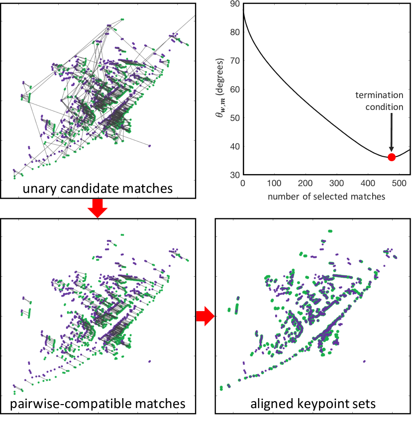
Our data association algorithm is an example of graph matching [24]. It seeks point correspondences based on global geometric constraints. Unlike ICP, which relies on the approximate alignment of scans, our method does not need prior knowledge of the relative displacement between scans. With no parameter tuning, it is easy to apply across datasets. Moreover, by formulating data association as a global optimization problem, our approach utilizes information across the entire scan and naturally removes outliers. Compared to [2], our current method is more efficient and robust due to changes to the unary keypoint descriptor and termination condition. As given in Algorithm 2, our approach takes in two keypoint sets and and proceeds in three stages.
Stage 1: Without loss of generality, assume . A unary candidate proposal method (see [2]) matches each keypoint to another , and the pair is added to (line 2). In this paper, we present a new rotation-invariant descriptor for keypoint . To compute :, we create a histogram of the number of elements in each angular slice around keypoint , take its fast Fourier transform, then normalize its phase. To compute :, we create a histogram of the number of elements in each annulus around keypoint , then normalize it. The angular slices and annuli have the same spatial resolution as the radar scan. Note that, as done in [2], each element contributing to the descriptor is weighted by its range relative to the radar to correct for radar’s range-density bias.
Stage 2: To refine the match proposals in , each pairwise combination of keypoints is compared to its associated (according to ) match pair . If and do indeed represent identical keypoints in the environment and the same holds true for and , then the pairwise relationships and must be similar, which is quantified by the compatibility score of the non-negative symmetric compatibility matrix (line 2). The formulation of this score is given in [2].
Stage 3: Maximizing the global compatibility score is done by finding the optimal match vector such that:
| (1) |
Logically, must satisfy the (i) integrality constraint: all elements are either or (i.e., a match is true or false) and (ii) uniqueness constraint (i.e., each keypoint in cannot maps to more than one keypoint in , and vice versa). We define such that if and otherwise, and let be the mapping between keypoint sets according to . This formulation is known as graph matching [24], and it is NP-hard, so we relax the constraints and solve instead for such that:
| (2) |
By the Raleigh’s ratio and Perron-Frobenius theorems [24], the solution is the principal eigenvector of . We use to approximate the optimal constrained solution to (1) via the greedy approach in lines 2-2. We present a new termination condition that stops adding matches when the new one is incompatible with those already in , as explained in Section IV-B. Compared to our previous work [2], the new condition is more robust and consistent because it does not depend on the magnitude of elements in .
The rigid-body motion (RBM) is found using a well-known technique [25]. As radar scans are in 2D, ego-motion is restricted to 3-DOF: planar translation and rotation.
IV System analysis
IV-A Algorithmic complexity
The complexity of our system is summarized in Table I. For most radars, . To estimate the average complexity, it is assumed that . The second row gives the complexity for data association with no prior on the relative motion between scans. When running the system in real time, because the relative motion between consecutive time steps is limited, a mild prior can be used to improve computational efficiency by reducing the number of unary descriptor comparisons. For this analysis, the intensity gradient, ordering, and principal eigenvector are computed using the Prewitt operator, merge sort, and power iteration, respectively.
Overall, the system computation is generally dominated by the unary candidate matching step in Stage 1 of data association, such that the average system complexity is given by . Because the bottleneck depends on , we intentionally allow to be set by the user as the only tunable input parameter of our system.
IV-B Theoretical analysis and performance measures
The fundamental principle behind our system is the optimization problem (1). Intuitively, it seeks the set of matches that maximizes the global compatibility score in (1). Because this problem is NP-hard, our algorithm approximates the optimal solution. This section investigates how well solution approximates . Let , where if and only if , and otherwise. is the corrected in which does not inflate the compatibility scores of , and can be considered a perturbation from due to incorrect matches.
Proposition 1
always overestimates the true global compatibility score, except when all proposed matches are correct (i.e., ), in which case they are equal.
Proof:
By definition of and , is non-negative: for any , or . ∎
Proposition 1 implies that match selection is overly optimistic, and it is more likely to add too many matches, some of which are bad, than to not add good ones. Therefore, when using , we seek to: (1) resolve conflicting proposed matches in order to satisfy the constraints on (1) by selecting the best of them, and (2) avoid adding poor matches. Our algorithm achieves the first goal by adding matches in order of largest corresponding value in . It achieves the second with the termination condition, explained next. Let be the compatibility matrix assuming perfect measurements.
Proposition 2
Assuming no perfect symmetry exists in the keypoint sets, .
Proof:
By Proposition 2, given the true compatibility matrix and optimal match set , the solution is, in fact, the binary vector even though no integral constraints are placed on . Since all accepted matches in are equally weighted, they are equally valued and agree with one another. We use this fact to seek a solution that, like , contains matches that are mutually consistent. By Proposition 1, the global compatibility score is an optimistic measure (i.e., does not imply that matches in are better than those in ). We use Proposition 2 to construct a more reliable measure, as follows.
Measure 1
The index measures the mutual compatibility of selected matches , where is the angle between vectors and .
Using this property, we terminate the greedy algorithm when the next match would cause to decreases. Intuitively, the new match would cause to move farther from its corresponding binary solution, where this separation is inversely related to the consistency between matches. Although similar to , the continuous values in scale match ’s contribution by its compatibility.
Measure 2
Assume the chosen solution is the optimal one: . Let represent the -th largest eigenvalue of . Then, the normalized eigengap measures the solution’s robustness to perturbations.
While is introspective (quantifies how well the selected matches agree), the second measure considers all proposed matches and quantifies the system’s confidence it its solution over the next-highest scoring solution.
| Average | Worst | |
|---|---|---|
| KE1 | ||
| DA | ||
| DA2 | ||
| ME3 |
-
1
Keypoint extraction
-
1
Data association with mild prior on relative motion
-
2
Rigid-body motion estimation
V Results
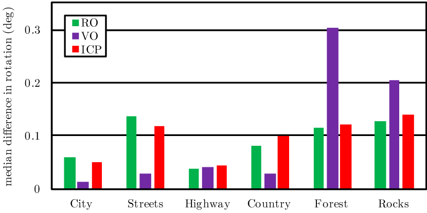
In [2], we demonstrate RO that performs comparably to VO and GPS (under ideal conditions for the latter two) and maintains precise odometry even under conditions for which VO and GPS fail. In this section, we build on this result and show that our new RO pipeline, which improves upon [2], achieves high accuracy in real time across diverse settings, from UK city streets to off-road landscapes in Iceland.
| Dataset | Setting1 | Avg. T. | Avg. R. | Dist. | RO |
|---|---|---|---|---|---|
| (m)2 | (deg)2 | (km) | Prior3 | ||
| City | Oxford, UK | 1.268 | 1.489 | 8.36 | None |
| Backstreets | Oxford, UK | 1.252 | 1.804 | 2.76 | None |
| Highway | M40, UK | 5.164 | 1.076 | 19.6 | Max. Acc. |
| Countryside | Rural UK | 2.297 | 1.264 | 16.8 | Max. Acc. |
| Forest | Heidmörk, IS | 3.168 | 0.769 | 9.37 | None |
| Rocks | Thórsmörk, IS | 1.267 | 1.036 | 2.35 | Max. Acc. |
-
1
UK and IS stand for the United Kingdom and Iceland, respectively.
-
2
These quantities are the average movement (in translation and rotation according to RO) between consecutive scans when the vehicle is not stationary. Scans are obtained at 4 Hz (i.e., speed is 4 times displacement).
-
3
“None” means that no motion prior is used during scan matching. “Max. Acc.” employs a very mild prior that limits the maximum distance the vehicle could have traveled based a maximum acceleration of 8 m/s2.
For keypoint extraction, we use . The six experimental datasets examined in this paper are described in Table II. As explained in the footnotes, the final column indicates whether a motion prior is used for RO. For three datasets, no motion prior is used at all. The other three employ a very mild motion prior that uses the system’s maximum possible acceleration of 8 m/s2 to remove impossible matches from consideration. Empirically, our system very rarely requires this prior (e.g., 2 scan matches out of 10,000). Incorrect alignments occur when the scene structure contains high levels of symmetry, resulting in many possible alignment solutions. The lenient prior serves to reduce the number of possible solutions. Due to space constraints, odometry plots for this work can be found in our video [26].
| Translation (m)1 | Rotation (deg)1 | |||
|---|---|---|---|---|
| Comparison | Median | Std. Dev. | Median | Std. Dev. |
| RO to GPS | 0.0520 | 0.0660 | 0.0929 | 0.1632 |
| RO to VO | 0.0724 | 0.0777 | 0.1414 | 0.2105 |
| VO to GPS2 | 0.0577 | 0.0546 | 0.1032 | 0.1396 |
-
1
Statistics for difference between estimated displacement (in translation and rotation) between consecutive radar scans, which are obtained at 4 Hz.
-
2
Contextualizes RO performance by comparing two well accepted methods.
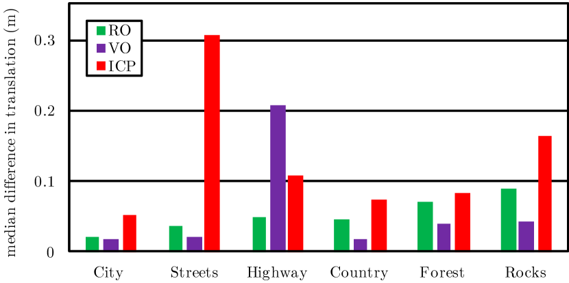
Fig. 5 evaluates RO performance against GPS and compares it to state-of-the-art VO [27] and popular scan matching method ICP. For ICP, we use a convergence tolerance of e-. We improve ICP performance by providing it with a good motion prior and limiting the possible matches to nearest neighbors within 2 m. Even so, RO outperforms ICP in every setting, as shown in Fig. 5(a). The occasional lower rotational error of ICP in Fig. 5(b) is misleading because it only occurs when ICP’s estimated translation is highly inaccurate, in which case the rotation error is meaningless. Relative to VO, RO generally achieves comparable though slightly lower accuracy, which can be explained by the fact that RO only captures 3-DOF motion compared to VO’s 6-DOF. Thus, if the platform experiences rolling or pitching, RO registers this motion into its 3-DOF estimate. Similarly, if the environment is less structured, variability in elevation is discarded in radar’s 2D scan, also affecting the resulting motion estimates. This reasoning is consistent with RO’s slightly higher error in countryside, forest, and boulder field (i.e., rocks) datasets. RO greatly outperforms VO on the highway, on which the average travel speed is highest, making radar odometry appealing from a safety perspective.
A summary of RO performance relative to GPS is given in Table IV, and a comparison of the three odometry methods using results averaged across all datasets is given in Table III. Table IV shows that our RO pipeline achieves high accuracy, differing from GPS by only 5.2 cm and 0.09 deg in translation and rotation, respectively, on average. Notably, the third row of Table III shows that the overall median difference between VO and GPS exceeds that between RO and GPS. On the other hand, the standard deviation of differences is larger for RO, meaning that RO provides highly precise yet slightly noisier motion estimates compared to VO. Importantly, as detailed in Table IV, RO is remarkably accurate in common settings (e.g., city center). Although the error seemingly increases for more complex environments (e.g., in Iceland), these discrepancies may be due to factors discussed in the previous paragraph.
This work achieves lower error in Oxford city compared to our previous work [2]. Though not shown, it consistently outperforms [2], which cannot handle unstructured settings.
| Translation (m) | Rotation (deg) | |||
|---|---|---|---|---|
| Setting | Median | Std. Dev. | Median | Std. Dev. |
| City | 0.0208 | 0.0318 | 0.0597 | 0.1442 |
| Backstreets | 0.0362 | 0.0398 | 0.1375 | 0.2238 |
| Highway | 0.0480 | 0.0598 | 0.0384 | 0.0673 |
| Countryside | 0.0462 | 0.0698 | 0.0811 | 0.1380 |
| Forest | 0.0711 | 0.0899 | 0.1141 | 0.1796 |
| Rocks | 0.0897 | 0.1050 | 0.1267 | 0.2267 |
VI Conclusion and Future Work
In this paper, we motivate the use of radar as an information-rich, long-range, and reliable sensor that is robust under challenging conditions. We propose keypoint extraction and scan matching algorithms that are designed to require minimal a priori knowledge and human intervention. We demonstrate our pipeline’s high accuracy across diverse settings, performing comparably and at times better than VO. We discuss our approach’s theoretical underpinnings, propose two performance measures, and analyze system complexity. Three areas of promising future work are: streamlining unary candidate proposal, addressing scene symmetry (e.g., using tertiary graph matching or quantifying motion observability), and deducing 3D information from 2D scans.
References
- [1] M. Adams and E. Jose, Robotic navigation and mapping with radar. Artech House, 2012.
- [2] S. H. Cen and P. Newman, “Precise ego-motion estimation with millimeter-wave radar under diverse and challenging conditions,” in Robotics and Automation, 2018. Proceedings. (ICRA 2018). 2018 IEEE International Conference on. IEEE, 2018.
- [3] S. H. Cen, “Ego-motion estimation and localization with millimeter-wave scanning radar,” Ph.D. dissertation, University of Oxford, Oxford, United Kingdom, 2019.
- [4] M. O. Aqel, M. H. Marhaban, M. I. Saripan, and N. B. Ismail, “Review of visual odometry: types, approaches, challenges, and applications,” SpringerPlus, vol. 5, no. 1, p. 1897, 2016.
- [5] D. Scaramuzza and F. Fraundorfer, “Visual odometry [tutorial],” IEEE robotics & automation magazine, vol. 18, no. 4, pp. 80–92, 2011.
- [6] J. Zhang and S. Singh, “Low-drift and real-time lidar odometry and mapping,” Autonomous Robots, vol. 41, no. 2, pp. 401–416, 2017.
- [7] R. W. Wolcott and R. M. Eustice, “Robust lidar localization using multiresolution gaussian mixture maps for autonomous driving,” The International Journal of Robotics Research, vol. 36, no. 3, pp. 292–319, 2017.
- [8] J. Borenstein, H. Everett, L. Feng et al., “Where am i? sensors and methods for mobile robot positioning,” University of Michigan, vol. 119, no. 120, p. 27, 1996.
- [9] L. Novak, “Correlation algorithms for radar map matching,” IEEE Transactions on Aerospace and Electronic Systems, no. 4, pp. 641–648, 1978.
- [10] P. Checchin, F. Gérossier, C. Blanc, R. Chapuis, and L. Trassoudaine, “Radar scan matching slam using the fourier-mellin transform,” in Field and Service Robotics. Springer, 2010, pp. 151–161.
- [11] D. Kellner, M. Barjenbruch, J. Klappstein, J. Dickmann, and K. Dietmayer, “Instantaneous ego-motion estimation using doppler radar,” in Intelligent Transportation Systems-(ITSC), 2013 16th International IEEE Conference on. IEEE, 2013, pp. 869–874.
- [12] M. Skolnik, Radar Handbook, Third Edition, ser. Electronics electrical engineering. McGraw-Hill Education, 2008. [Online]. Available: https://books.google.co.uk/books?id=76uF2Xebm-gC
- [13] K. Werber, J. Klappstein, J. Dickmann, and C. Waldschmidt, “Interesting areas in radar gridmaps for vehicle self-localization,” in Microwaves for Intelligent Mobility (ICMIM), 2016 IEEE MTT-S International Conference on. IEEE, 2016, pp. 1–4.
- [14] F. Lu and E. Milios, “Robot pose estimation in unknown environments by matching 2d range scans,” Journal of Intelligent and Robotic systems, vol. 18, no. 3, pp. 249–275, 1997.
- [15] M. Rapp, M. Barjenbruch, M. Hahn, J. Dickmann, and K. Dietmayer, “Clustering improved grid map registration using the normal distribution transform,” in Intelligent Vehicles Symposium (IV), 2015 IEEE. IEEE, 2015, pp. 249–254.
- [16] J. Callmer, D. Törnqvist, F. Gustafsson, H. Svensson, and P. Carlbom, “Radar slam using visual features,” EURASIP Journal on Advances in Signal Processing, vol. 2011, no. 1, p. 71, 2011.
- [17] P. J. Besl, N. D. McKay et al., “A method for registration of 3-d shapes,” IEEE Transactions on pattern analysis and machine intelligence, vol. 14, no. 2, pp. 239–256, 1992.
- [18] M. Yang, B. Dong, H. Wang, and B. Zhang, “Laser radar based real-time ego-motion estimation for intelligent vehicles,” in Intelligent Vehicle Symposium, 2002. IEEE, vol. 1. IEEE, 2002, pp. 44–51.
- [19] M. Rapp, M. Barjenbruch, M. Hahn, J. Dickmann, and K. Dietmayer, “Probabilistic ego-motion estimation using multiple automotive radar sensors,” Robotics and Autonomous Systems, vol. 89, pp. 136–146, 2017.
- [20] M. Chandran and P. Newman, “Motion estimation from map quality with millimeter wave radar,” in Intelligent Robots and Systems, 2006 IEEE/RSJ International Conference on. IEEE, 2006, pp. 808–813.
- [21] D. Vivet, P. Checchin, and R. Chapuis, “Localization and mapping using only a rotating fmcw radar sensor,” Sensors, vol. 13, no. 4, pp. 4527–4552, 2013.
- [22] F. Schuster, C. G. Keller, M. Rapp, M. Haueis, and C. Curio, “Landmark based radar slam using graph optimization,” in Intelligent Transportation Systems (ITSC), 2016 IEEE 19th International Conference on. IEEE, 2016, pp. 2559–2564.
- [23] F. Schuster, M. Wörner, C. G. Keller, M. Haueis, and C. Curio, “Robust localization based on radar signal clustering,” in Intelligent Vehicles Symposium, 2016 IEEE. IEEE, 2016, pp. 839–844.
- [24] M. Leordeanu and M. Hebert, “A spectral technique for correspondence problems using pairwise constraints,” in Computer Vision, 2005. ICCV 2005. Tenth IEEE International Conference on, vol. 2. IEEE, 2005, pp. 1482–1489.
- [25] J. H. Challis, “A procedure for determining rigid body transformation parameters,” Journal of biomechanics, vol. 28, no. 6, pp. 733–737, 1995.
- [26] S. H. Cen and P. Newman, “Radar-only ego-motion estimation in difficult settings via graph matching,” YouTube Spotlight Video for ICRA, 2019.
- [27] W. Churchill, “Experience based navigation: Theory, practice and implementation,” Ph.D. dissertation, University of Oxford, Oxford, United Kingdom, 2012.