Diffusion and universal relaxation of holographic phonons

Abstract

In phases where translations are spontaneously broken, new gapless degrees of freedom appear in the low energy spectrum (the phonons). At long wavelengths, they couple to small fluctuations of the conserved densities of the system. This mixing is captured by new diffusive transport coefficients, as well as qualitatively different collective modes, such as shear sound modes. We use Gauge/Gravity duality to model such phases and analytically compute the corresponding diffusivities in terms of data of the dual background black hole solution. In holographic quantum critical low temperature phases, we show that these diffusivities are governed by universal relaxation of the phonons into the heat current when the dynamical critical exponent $z>2$. Finally, we compute the spectrum of transverse collective modes and show that their dispersion relation matches the dispersion relation of the shear sound modes of the hydrodynamic theory of crystalline solids.

1 Introduction

One of the most celebrated results originating from Gauge/Gravity duality Maldacena:1997re ; Ammon:2015wua ; Zaanen:2015oix ; Hartnoll:2016apf is the computation of the shear viscosity of the $\mathcal{N}=4$ super Yang-Mills plasma at infinite $N$ ($N$ is the rank of the gauge group) and ’t Hooft coupling in terms of the entropy density of a dual black hole in anti de Sitter spacetime, $\eta=s/4\pi$ (in natural units) Policastro:2001yc . This was conjectured to place a lower bound on the ratio $\eta/s\gtrsim 1/4\pi$ for strongly-coupled phases of matter Kovtun:2004de . Recalling that the entropy density is proportional to the area of the bulk black hole, this relation is universal in the sense that the complicated dependence on the boundary sources is encapsulated as a simple combination of data defined at the black hole horizon Iqbal:2008by .

In a relativistic plasma, which is described at long wavelengths by relativistic hydrodynamics (see Kovtun:2012rj for a review of relativistic hydrodynamics), the shear viscosity controls the diffusion of transverse momentum $D_{\perp}=\eta/(\epsilon+p)$, where $\epsilon$ and $p$ are the energy density and pressure.

At nonzero density, relativistic hydrodynamics predicts the existence of another, incoherent diffusion constant $\sigma_{0}$, associated to processes without any momentum drag. This diffusivity can also be computed in terms of horizon data Davison:2015taa ; Davison:2018ofp ; Davison:2018nxm , as well as the thermal diffusivity that governs energy diffusion Blake:2017qgd .

Taken together, these results point at an interesting link between universal low energy transport properties (diffusivities) and the dynamics close to black hole horizons.

These results have been extended to less symmetric cases describing inhomogeneous states, such as the so-called holographic lattices that break translations explicitly with a periodic potential Donos:2014yya ; Donos:2015gia ; Banks:2015wha . At long distances, charge and energy diffuse in these inhomogeneous systems Hartnoll:2014lpa ; Donos:2017gej . The diffusivities are proportional to the dc thermoelectric conductivities of the system via Einstein relations, which relates them to horizon data under very general assumptions Donos:2017ihe .

More recent developments have considered the effect of breaking translations spontaneously in one or more spatial directions, which can be implemented either in a homogeneous Amoretti:2016bxs ; Alberte:2017oqx ; Amoretti:2017frz ; Amoretti:2017axe or an inhomogeneous way Ooguri:2010kt ; Donos:2011bh ; Donos:2013wia ; Withers:2013loa ; Jokela:2014dba ; Jokela:2016xuy . In either case, the incoherent conductivity and associated diffusivity of the boundary theory can be expressed in terms of horizon data for thermodynamically stable phases Amoretti:2017frz ; Amoretti:2017axe ; Donos:2018kkm ; Gouteraux:2018wfe . For thermodynamically unstable phases, the incoherent conductivity also features an integral over the whole spacetime of some combination of background fields.

The effective theory chaikin_lubensky_1995 ; Delacretaz:2017zxd capturing the low energy dynamics of such states with spontaneous translation symmetry breaking contains more than the two characteristic diffusivities just mentioned, due to the presence of additional gapless degrees of freedom (the Goldstones of spontaneous translation symmetry breaking or in other words, the phonons) and their mixing with charge and energy fluctuations. The theory of Wigner crystal (WC) hydrodynamics is succinctly reviewed in section 2 and the diffusivities we are interested in are presented there. Then, in section 3, we give some details of our holographic setup. A first objective of this work is to extend previous analyses and show that all of these diffusivities can be expressed in terms of the background black hole solution, by a combination of data on the horizon and on the rest of the spacetime. This is done in section 4, and our main new results are equations (64) and (65).

Positivity of entropy production in WC hydrodynamics places a bound on a combination of the diffusivities, see equation (9). The holographic diffusivities obey this bound, as we discuss in section 5. Interestingly, this bound can be saturated at low temperatures. This obtains when the phonons relax into the heat current and leads to simple relations between the diffusivities. We expect this universal relaxation channel to be at play in generic states of matter at finite temperature. We give a criterion for the saturation of this bound as a function of the values of the scaling exponents characterizing the infra-red fixed point of the system and the irrelevant deformations away from it. Universal relaxation of phonons into a hydrodynamic operator has also been recently discussed in the context of the melting of the field-induced Wigner solid in Delacretaz:2019 .

In section 6, we conclude with an analysis of the spectrum of the system at nonzero wavevector by computing the longest-lived pair of transverse quasinormal modes (QNMs) of the dual black hole. We show that they obey the expected dispersion relation from WC hydrodynamics. At low wavevector and intermediate temperatures, there is a pair of shear sound modes, characteristic of the long wavelength dynamics of solids. However, either at very low or very high temperatures, these modes collide on the imaginary frequency axis and become pseudo-diffusive, with a purely imaginary gap controlled by a ratio of thermodynamic data and diffusivities. Both collisions occur in the hydrodynamic regime and the dispersion relation of the modes is well-captured by the hydrodynamic dispersion relation, see equation (79). These results were originally presented in Amoretti:2018tzw , but have been moved and expanded upon in the present work for clarity.

We give a number of technical digressions as well as details of our numeric scheme in some appendices.

2 Review of Wigner crystal hydrodynamics

We first recap the main features of two-dimensional isotropic Wigner crystal hydrodynamics. More details can be found in chaikin_lubensky_1995 ; Delacretaz:2017zxd . As translations are broken spontaneously along both spatial directions, the usual conserved densities (energy, charge, momentum) need to be coupled to two Goldstone modes, $\varphi_{i}$, $i=x,y$. The free energy is supplemented by terms capturing the effect of the Goldstones:

$$f=\frac{1}{2}K|q\cdot\varphi_{q}|^{2}+\frac{1}{2}Gq^{2}|\varphi_{q}|^{2}\,.$$ (1)

$K$ and $G$ are the bulk and shear moduli, and characterize the stiffness of phase fluctuations around the ordered state. It is convenient to parameterize the Goldstones by their longitudinal and transverse contributions, $\lambda_{\parallel}=\nabla\cdot\varphi$ and $\lambda_{\perp}=\nabla\times\varphi$. The corresponding sources $s_{\parallel,\perp}$ are defined by requiring that $\lambda_{\parallel,\perp}=\delta f/\delta s_{\parallel,\perp}$.

To leading order in gradients and keeping only linear terms, the Goldstones obey the following ‘Josephson’ relations

$$\begin{split}\partial_{t}\lambda_{\parallel}=&\nabla\cdot v+\gamma_{1}\nabla^{2}\mu+\gamma_{2}\nabla^{2}T+\frac{\xi_{\parallel}}{K+G}\nabla^{2}s_{\parallel}+\dots\,,\\ \partial_{t}\lambda_{\perp}=&\nabla\times v+\frac{\xi_{\perp}}{G}\nabla^{2}s_{\perp}+\dots\,,\end{split}$$ (2)

where $v$ is the velocity, $\mu$ the chemical potential, and $\gamma_{1,2}$ and $\xi_{\parallel,\perp}$ are diffusive transport coefficients.

These equations are supplemented by current, heat and momentum conservation equations (energy can be traded for entropy to linear order):

$$\partial_{t}\rho+\nabla\cdot j=0\,,\quad\partial_{t}s+\nabla\cdot(j_{q}/T)=0\,,\quad\partial\pi^{i}+\nabla_{j}T^{ji}=0\,,$$ (3)

together with the constitutive relations

$$\begin{split}j=&\rho v-\sigma_{o}\nabla\mu-\alpha_{o}\nabla T-\gamma_{1}\nabla s_{\parallel}+\dots\,,\\ j_{q}/T=&sv-\alpha_{o}\nabla\mu-(\bar{\kappa}_{o}/T)\nabla T-\gamma_{2}\nabla s_{\parallel}+\dots\,,\\ T^{ij}=&\delta^{ij}\left(p+(K+G)\nabla\cdot\varphi\right)+2G\left[\nabla^{(i}\varphi^{j)}-\delta^{ij}\nabla\cdot\varphi\right]-\eta\left(2\nabla^{(i}v^{j)}-\delta^{ij}\nabla\cdot v\right)+\dots\end{split}$$ (4)

The underlying conformal symmetry of the holographic setup implies that the stress-energy tensor is traceless, which sets the bulk viscosity to zero.

The hydrodynamic retarded Green’s functions at nonzero frequency and wavevector are derived by following the Kadanoff-Martin procedure 1963AnPhy..24..419K ; Kovtun:2012rj :

$$G^{R}_{AB}(\omega,q)=M_{AC}\left[\left(i\omega-M\right)^{-1}\right]_{CD}\chi_{DB}$$ (5)

where the vevs $A,B=(\delta\rho,\delta s,\pi_{\parallel},\lambda_{\parallel},\pi_{\perp},\lambda_{\perp})$ and the corresponding sources are
$(\delta\mu,\delta T,v_{\parallel},s_{\parallel},v_{\perp},s_{\perp})$. $M$ is the matrix

$$M_{AB}=\left(\begin{array}[]{cccccc}\sigma_{o}q^{2}&\alpha_{o}q^{2}&i\rho q&\gamma_{1}q^{2}&0&0\\ \alpha_{o}q^{2}&\frac{\bar{\kappa}_{o}}{T}q^{2}&isq&\gamma_{2}q^{2}&0&0\\ i\rho q&isq&\eta q^{2}&iq&0&0\\ \gamma_{1}q^{2}&\gamma_{2}q^{2}&iq&\frac{\xi_{\parallel}}{K+G}q^{2}&0&0\\ 0&0&0&0&\eta q^{2}&iq\\ 0&0&0&0&iq&\frac{\xi_{\perp}}{G}q^{2}\end{array}\right)\,.$$ (6)

Relativistic symmetry of the holographic setup enforces that the momentum and energy current densities must be equal $\pi=j_{e}$, which places constraints on the transport coefficients:

$$\alpha_{o}=-\frac{\mu}{T}\sigma_{o}\,,\quad\bar{\kappa}_{o}=\frac{\mu^{2}}{T}\sigma_{o}\,,\quad\gamma_{2}=-\frac{\mu}{T}\gamma_{1}\,.$$ (7)

Observe that this also means that the heat current $j_{q}\equiv j_{e}-\mu j=\pi-\mu j$. Finally, the susceptibility matrix is

$$\chi_{AB}=\left(\begin{array}[]{cccccc}\chi_{\rho\rho}&\chi_{\rho s}&0&0&0&0\\ \chi_{\rho s}&\chi_{ss}&0&0&0&0\\ 0&0&\chi_{\pi\pi}&0&0&0\\ 0&0&0&\frac{1}{K+G}&0&0\\ 0&0&0&0&\chi_{\pi\pi}&0\\ 0&0&0&0&0&\frac{1}{G}\end{array}\right)\,.$$ (8)

Positivity of entropy production can be ensured by requiring all the eigenvalues of the matrix $M$ to be positive Delacretaz:2017zxd , which leads to the following constraints:

$$\eta\geq 0\,,\qquad\sigma_{o}\geq 0\,,\qquad\gamma_{1}^{2}\leq{\frac{\sigma_{o}\xi_{\parallel}}{K+G}}\,.$$ (9)

Using (5) and identities between the Green’s functions stemming from (3), we obtain in the $q\to 0$ limit

$$G^{R}_{T^{xy}T^{xy}}=G-i\omega\eta\,,$$ (10)

$$G^{R}_{jj}=\frac{\rho^{2}}{\chi_{\pi\pi}}-i\omega\sigma_{o}\,,\quad\quad G^{R}_{j\pi_{\parallel}}=\rho\,,\quad\quad G^{R}_{j\varphi_{\parallel}}=-\gamma_{1}-\frac{i\rho}{\chi_{\pi\pi}\,\omega}\,,$$ (11)

$$G^{R}_{\pi_{\parallel}\varphi_{\parallel}}=G^{R}_{\varphi_{\parallel}\pi_{\parallel}}=\frac{i}{\omega}\,,\quad G^{R}_{\varphi_{\parallel}\varphi_{\parallel}}=\frac{1}{\chi_{\pi\pi}\,\omega^{2}}-\frac{\xi_{\parallel}}{K+G}\frac{i}{\omega}\,,\quad G^{R}_{\varphi_{\perp}\varphi_{\perp}}=\frac{1}{\chi_{\pi\pi}\,\omega^{2}}-\frac{\xi_{\perp}}{G}\frac{i}{\omega}\,.$$ (12)

We defined e.g.

$$G^{R}_{\varphi_{i}\varphi_{j}}=\frac{q_{i}q_{j}}{q^{4}}G^{R}_{\lambda_{\parallel}\lambda_{\parallel}}+\left[\delta_{ij}-\frac{q_{i}q_{j}}{q^{2}}\right]\frac{G^{R}_{\lambda_{\perp}\lambda_{\perp}}}{q^{2}}\,,$$ (13)

and

$${q^{2}G^{R}_{\varphi_{\parallel}\varphi_{\parallel}}=G^{R}_{\lambda_{\parallel}\lambda_{\parallel}}\,,\quad q^{2}G^{R}_{\varphi_{\perp}\varphi_{\parallel}}=G^{R}_{\lambda_{\perp}\lambda_{\perp}}}\,.$$ (14)

In this $q=0$ limit, for an isotropic crystal, $G^{R}_{\lambda_{\parallel}\lambda_{\parallel}}=G^{R}_{\lambda_{\perp}\lambda_{\perp}}$, since there should be no distinction between the longitudinal and tranverse phonons. This leads to the constraint

$$\frac{\xi_{\parallel}}{K+G}=\frac{\xi_{\perp}}{G}\equiv X\,.$$ (15)

3 Holographic model

3.1 Setup

We consider the holographic model

$$S=\int d^{4}x\,\sqrt{-g}\left[R-\frac{1}{2}\partial\phi^{2}-V(\phi)-\frac{1}{4}Z(\phi)F^{2}-\frac{1}{2}\sum_{I=1}^{2}Y(\phi)\partial\psi_{I}^{2}\right],$$ (16)

with the scalar couplings behaving near the AdS boundary, i.e. in the small $\phi$ limit, as

$$V_{uv}(\phi)=-6-\phi^{2}+O(\phi^{3})\,,\quad Z_{uv}(\phi)=1+O(\phi)\,,\quad Y_{uv}(\phi)=\phi^{2}+O(\phi^{3})\,.$$ (17)

The model (16) enjoys a global shift symmetry $\psi_{I}\mapsto\psi_{I}+c_{I}$. In this work, we will be interested in states that break translations homogeneously Donos:2013eha ; Andrade:2013gsa , with

$$\psi_{I}=kx^{I}\,,\quad x^{I}=\{x,y\}\,.$$ (18)

This Ansatz breaks the shift symmetry as well as spacetime translations to a diagonal U(1). As a consequence, the background metric, scalar $\phi$ and gauge field only depend on the holographic radial coordinate,

$$ds^{2}=-D(r)dt^{2}+B(r)dr^{2}+C(r)(dx^{2}+dy^{2}),\quad\phi=\phi(r),\quad A=A(r)dt\,.$$ (19)

$t,x,y$ are the time and space coordinates of the dual field theory. Given (17) and (18), the dual boundary theory is deformed by two complex scalar operators $\Phi_{I}\simeq\phi e^{i\psi_{I}}$ . These deformations break translations through the spatial dependence of the phases $\psi_{I}$.

As explained in Amoretti:2016bxs ; Amoretti:2017frz ; Amoretti:2017axe , whether translations are broken explicitly or spontaneously in the boundary theory depends on the asymptotic behaviour of the scalar $\phi$ near the AdS boundary. For our choice of scalar potential, $\phi$ decays towards the boundary as

$$\phi(r\to 0)=\lambda r+\phi_{(v)}r^{2}+O(r^{3})\,.$$ (20)

In the usual quantization scheme, $\lambda$ is the source of the operator dual to the bulk field $\phi$ and $\phi_{(v)}$ is related to its vev. If $\lambda=0$, the breaking is spontaneous. If $\lambda\neq 0$, it is explicit. In this work we will only consider the spontaneous case.

The condensation of the order parameter itself (i.e. the phase transition between the normal and ordered phase) is not captured by the model. This is typically mediated by an instability towards a spatially modulated, inhomogeneous phase which minimizes the free energy, Donos:2013wia ; Withers:2013loa ; Withers:2014sja ; Jokela:2016xuy . Instead, the holographic model (16) with zero scalar source $\lambda=0$ directly describes the low energy dynamics of the phonons in the ordered phase, as we shall demonstrate in the remainder of this work. As we show below, the fluctuations of the bulk fields $\psi_{I}$ are dual to the phonons. The bulk global symmetry should then be understood as encoding the shift symmetry of the NG bosons, not as a symmetry of the fundamental UV theory.

Finite temperature, finite density states are modeled by charged black holes in the bulk, which implies the existence of a regular black hole horizon at $r=r_{h}$. In the rest of this work, we use a subscript $h$ to denote quantities evaluated at $r=r_{h}$. The temperature $T$ and the entropy density $s$ are given by:

$$s=4\pi C(r_{h})\ ,\qquad T=\frac{1}{4\pi}\left.\sqrt{-\frac{B^{\prime}(r)D^{\prime}(r)}{B(r)^{2}}}\right|_{r=r_{h}}\ ,$$ (21)

with the following near-horizon expansion

$$\begin{split}&ds^{2}=-4\pi T(r_{h}-r)dt^{2}+\frac{dr^{2}}{4\pi T(r_{h}-r)}+\frac{s}{4\pi}(dx^{2}+dy^{2})+\dots\ ,\\ &A_{t}=A_{h}(r_{h}-r)+\dots\ ,\qquad\phi=\phi_{h}+\dots\ .\end{split}$$ (22)

We will also be interested in the low temperature behaviour $T\ll\mu$ (where $\mu$ is the chemical potential) of these translation-breaking black holes. More precisely, we would like to study the interplay between spontaneous translation symmetry breaking and quantum criticality. To do so, we will assume that the scalar $\phi$ has a runaway behaviour as $T\to 0$ and $r\to+\infty$ (or equivalently that the horizon value of the scalar diverges at low temperature), and that the scalar couplings behave for large $\phi$ as

$$V(\phi\to\infty)=V_{0}e^{-\delta\phi}\ ,\quad Z(\phi\to\infty)=Z_{0}e^{\gamma\phi}\ ,\quad Y_{IR}=Y(\phi\to\infty)e^{\nu\phi}\,.$$ (23)

The near-extremal, near-horizon geometry of the black hole is then described by a Lifshitz, hyperscaling-violating solution

$$\begin{split}&ds^{2}=\xi^{\theta}\left[-f(\xi)\frac{dt^{2}}{\xi^{2z}}+\frac{L^{2}d\xi^{2}}{\xi^{2}f(\xi)}+\frac{d\vec{x}^{2}}{\xi^{2}}\right],\quad f(\xi)=1-\left(\frac{\xi}{\xi_{h}}\right)^{2+z-\theta}\,,\\ &A=A_{o}\,\xi^{\theta-2-z}dt\ ,\quad\psi_{I}=k\delta_{Ii}x^{i}\,,\quad\phi=\kappa\log\xi\,.\end{split}$$ (24)

$\xi$ is a radial coordinate valid close to $r_{h}$, simultaneously taking the small temperature limit $T\ll\mu$. $\xi_{h}$ is the location of a Killing event horizon, with the associated Hawking temperature $T\sim\xi_{h}^{-1/z}$ and Hawking-Bekenstein entropy $s\sim\xi_{h}^{\theta-2}$. Combining both formulæ the entropy density scales as $s\sim T^{\frac{2-\theta}{z}}$. More details of these solutions can be found in Gouteraux:2014hca or more recently Davison:2018nxm . Here, we simply recall that in general the couplings appearing in (23) are related to the scaling exponents characterizing the solution as

$$\kappa\delta=\theta\,,\qquad\kappa\gamma=4-\theta-2\Delta_{A_{o}}\,,\qquad\kappa\nu=2\Delta_{k}-2\,.$$ (25)

The exponents $\Delta_{A_{o},k}\leq 0$ are the scaling dimension of sources of irrelevant operators breaking particle/hole symmetry or translations of the IR $T=0$ critical solution.

For concreteness, in our numerical calculations we work with

$$V(\phi)=-6\cosh(\phi/\sqrt{3})\,,\quad Z(\phi)=\exp(-\phi/\sqrt{3})\,,\quad Y(\phi)=(1-\exp\phi)^{2}\,.$$ (26)

This implies that the critical solution (24) is characterized by $\theta\to-\infty$, $z\to+\infty$, $-\theta/z=1$ and $\Delta_{A_{o},k}=0$. As a consequence, it has a vanishing entropy density $s\sim T$. Our results can easily be generalized to other scalings. The numerical results presented in this paper are for $k/\mu=0.1$ and $\lambda=0$.

3.2 Holographic renormalization

Holographic renormalization for the spontaneous case was explained in Amoretti:2017frz , to which we refer for details. The salient features are the following. The UV expansion of the fields $\psi_{I}$ are modified compared to that of ordinary massless scalars due to their coupling to the scalar $\phi$. If $\phi$ is not sourced $\lambda=0$, then close to the AdS boundary $r\to 0$

$$\psi_{I}=\frac{\psi_{I,(-1)}}{r}+\psi_{I,(0)}+O(r)=\frac{1}{r^{2}}\left(\psi_{I,(-1)}r+\psi_{I,(0)}r^{2}+O(r^{3})\right)\,,$$ (27)

where we have used that the operator dual to $\phi$ has dimension $\Delta=2$ due to (26). This makes clear that the operators dual to the $\psi_{I}$ have the same scaling dimension as the operator dual to $\phi$ and that the whole scalar sector of deformations of the UV CFT is better understood as complex scalar operators dual to bulk complex scalar fields $\Phi_{I}\simeq\phi e^{i\psi_{I}}$ for small $\phi$ (ie close to the AdS boundary). $\phi$ and the $\psi_{I}$ are respectively the modulus and phase of the complex scalar, and inherit its scaling dimension. See Amoretti:2017frz for details. Going back to our background Ansatz (18), we see that indeed this corresponds to spontaneous translation breaking, since the source term $\psi_{(-1)}$ is not turned on. These powers can be generalized easily to the case $\Delta\neq 2$ and spatial dimension $d\neq 2$.

Near the boundary, the metric and gauge field behave in Fefferman-Graham gauge as

$$\begin{split}&D(r)=\frac{1}{r^{2}}\left(1+d_{(3)}r^{3}+O(r^{4})\right)\ ,\quad C(r)=\frac{1}{r^{2}}\left(1-\frac{d_{(3)}}{2}r^{3}+O(r^{4})\right),\\ &B(r)=\frac{1}{r^{2}}\ ,\hskip 119.50148ptA(r)=\mu-\rho r+O(r^{3})\,,\end{split}$$ (28)

where subleading coefficients are fixed in terms of, $\rho$, $\phi_{(v)}$ and $d_{(3)}$. This allows to read off the one-point correlation functions of the dual field theory, after computing the on-shell action renormalized by suitable counterterms deHaro:2000vlm . We find Amoretti:2017frz

$$\begin{split}\langle T^{tt}\rangle=\epsilon=-3d_{(3)}\,,\quad&\langle T^{xx}\rangle=\langle T^{yy}\rangle=-\frac{3}{2}d_{(3)}\\ &\langle J^{t}\rangle=\rho\ ,\quad\langle O_{\phi}\rangle=\phi_{(v)}\,.\end{split}$$ (29)

Another useful relation is

$$sT=-\mu\rho-\frac{9d_{(3)}}{2}-k^{2}\int_{0}^{r_{h}}dr\,\sqrt{BD}Y\,,$$ (30)

which results from evaluating the radially conserved bulk expression

$$\left[\rho A(r)+\frac{C^{2}(r)}{\sqrt{B(r)D(r)}}\left(\frac{D(r)}{C(r)}\right)^{\prime}-k^{2}\int_{r}^{r_{h}}d\tilde{r}\,\sqrt{BD}Y\right]^{\prime}=0\,.$$ (31)

both at the horizon and at the boundary. This is the Noether charge associated to the bulk time-like Killing vector Papadimitriou:2005ii ; Gouteraux:2018wfe . By evaluating the on-shell action for the background solution, we also find that $p=sT+\mu\rho-\epsilon$.

From the analysis above, $\chi_{\pi\pi}$ was obtained exactly in $k$ Amoretti:2017frz ; Amoretti:2017axe :

$$\chi_{\pi\pi}=sT+\mu\rho+k^{2}I_{Y}\,,\quad I_{Y}=\int_{0}^{r_{h}}dr\,\sqrt{BD}Y\,.$$ (32)

In this paper, we will only be interested in the transverse sector of fluctuations $\delta g_{t}^{x}(r,t,x)=\delta h_{t}^{x}(r)e^{-i\omega t+iqy}$, $\delta g_{x}^{y}(r,t,x)=\delta h_{x}^{y}(r)e^{-i\omega t+iqy}$, $\delta g_{r}^{x}(r,t,x)=\delta h_{r}^{x}(r)e^{-i\omega t+iqy}$, $\delta a_{x}(r,t,x)=\delta a_{x}(r)e^{-i\omega t+iqy}$ and $\delta\psi_{x}(r,t,x)=\delta\psi_{x}(r)e^{-i\omega t+iqy}$. We have used the homogeneity of our Ansatz to expand the fluctuations in plane waves. In the radial gauge $\delta g_{r}^{x}=0$, and setting $q=0$ for now, their boundary expansions are

$$\begin{split}&\delta a_{x}(r)=\delta a_{(0)}+\delta a_{(1)}r+\dots\,,\\ &\delta h_{t}^{x}(r)=\delta h_{1,(0)}+\delta h_{1,(3)}r^{3}+\dots\,,\\ &\delta h_{x}^{y}(r)=\delta h_{2,(0)}+\delta h_{2,(3)}r^{3}+\dots\,,\\ &\delta\psi_{x}(r)=\frac{1}{r}\left(\delta\psi_{(-1)}+\delta\psi_{(0)}r+\dots\right)\,,\end{split}$$ (33)

where $(\delta a_{(0)},\delta h_{1,(0)},\delta h_{2,(0)},\delta\psi_{(-1)})$ are sources and $(\delta a_{(1)},\delta h_{1,(3)},\delta h_{2,(3)},\delta\psi_{(0)})$ are vevs.

Then, the renormalized action at quadratic order in the fluctuations reads:

$$\begin{split}S_{\rm ren}^{(2)}=\int d\omega&\left[\delta a_{(0)}\delta a_{(1)}-\rho\delta a_{(0)}\delta h_{1,(0)}-\frac{3}{2}\delta h_{1,(0)}\delta h_{1,(3)}\right.\\ &\left.+\frac{3}{2}d_{(3)}(\delta h_{1,(0)})^{2}+(\phi_{(v)})^{2}\delta\psi_{(-1)}\delta\psi_{(0)}-\frac{3}{2}\delta h_{2,(0)}\delta h_{2,(3)}+\frac{3}{2}d_{(3)}(\delta h_{2,(0)})^{2}\right].\end{split}$$ (34)

3.3 AC boundary correlators

The Goldstone modes can be identified by acting on the background with the Lie derivative along $\partial/\partial_{\vec{x}}$. It leaves all fields invariant except the $\psi_{I}$’s. This confirms that phonon dynamics are captured by the fluctuations $\delta\psi_{I}$, and by computing the retarded Green’s functions in the limit $\omega\neq 0$, $q=0$, we will verify that they take the expressions predicted by WC hydrodynamics (10), (11) and (12).

At zero density, we can solve the equations analytically in the low frequency limit and confirm that we correctly obtain the zero density hydrodynamic correlators (12) in appendix A. At nonzero density, we made this check numerically, and we describe our numerical methods in appendix B.

The outcome of this analysis is that we identify the boundary phonon and its source along the direction $i={x,y}$ as

$$\varphi_{i}=\frac{\delta\psi_{i,(0)}}{k(\phi_{(v)})^{2}}\,,\quad\delta s_{\varphi,i}=k(\phi_{(v)})^{2}\delta\psi_{i,(-1)}\,.$$ (35)

Suppressing the spatial index, they appear in the on-shell action (34) as

$$\begin{split}S_{\rm ren}^{(2)}=\int d\omega&\left[\delta a_{(0)}\delta a_{(1)}-\rho\delta a_{(0)}\delta h_{1,(0)}-\frac{3}{2}\delta h_{1,(0)}\delta h_{1,(3)}\right.\\ &\left.+\frac{3}{2}d_{(3)}(\delta h_{1,(0)})^{2}+(\phi_{(v)})^{2}\varphi\delta s_{\varphi}-\frac{3}{2}\delta h_{2,(0)}\delta h_{2,(3)}+\frac{3}{2}d_{(3)}(\delta h_{2,(0)})^{2}\right].\end{split}$$ (36)

Once we have determined the on-shell action for the fluctuations $\delta a_{x}$, $\delta\psi_{x}$, $\delta g_{t}^{x}$, it is easy to compute the boundary correlators encoded in those bulk fluctuations Kaminski:2009dh . This entails numerically solving the relevant equations of motion as we describe in appendix B.2. We then verify that the zero frequency limit of those correlators matches the hydrodynamic expressions (11) and (12) for the retarded Green’s functions $G^{R}_{AB}(\omega\to 0,q=0)$. $A,B={j^{x},\pi^{x},\varphi_{x}}$, where $\chi_{\pi\pi}$ is given by (32). In section 4, we also obtain expressions for the diffusivities $\sigma_{o}$, $X$ and $\gamma_{1}$ (introduced in (6), (15)) which give an excellent match to the correlators. Their expressions are given in (63)-(65).

3.4 Shear modulus and shear viscosity

We will now evaluate the shear modulus and the shear viscosity holographically using the low frequency shear correlator (10). The low frequency behavior of the shear correlator can be computed analytically in a standard way, following Lucas:2015vna ; Davison:2015taa ; Hartnoll:2016tri (see Alberte:2017cch ; Alberte:2017oqx ; Baggioli:2018bfa for computations of the shear correlator in spontaneous holographic setups, Alberte:2015isw ; Alberte:2016xja ; Burikham:2016roo ; Ciobanu:2017fef in explicit setups). The equation of motion for the metric perturbation $h_{x}^{y}=h_{2}(r)e^{-i\omega t}$:

$$\left(\sqrt{\frac{D}{B}}Ch_{2}^{\prime}\right)^{\prime}-k^{2}Y(\phi)\sqrt{BD}h_{2}+\omega^{2}\sqrt{\frac{B}{D}}Ch_{2}=0\ .$$ (37)

Setting $\omega=0$, there are two linearly independent solutions, one regular $h^{(reg)}_{2}$ at the horizon and one singular $h^{(sing)}_{2}$. The singular solution can be expressed from the regular one

$$h^{(sing)}_{2}=h^{(reg)}_{2}\int^{r}_{0}\frac{\sqrt{B}}{\sqrt{D}C\left(h^{(reg)}_{2}\right)^{2}}\ ,$$ (38)

and behaves near the horizon as

$$h^{(sing)}_{2}(r_{h})\sim-\frac{\log(r_{h}-r)}{sTh_{2}^{(reg)}(r_{h})}+\textrm{finite}.$$ (39)

When $k\neq 0$, the regular solution can only be found perturbatively in $k$:

$$h^{(reg)}_{2}(r)=1-k^{2}\int_{0}^{r}dr_{1}\sqrt{\frac{B}{D}}\frac{1}{C}\int^{r_{h}}_{r_{1}}\sqrt{BD}Y+O(k^{4})\,.$$ (40)

At the horizon we should impose ingoing boundary conditions

$$h_{2}(r)=h^{(reg)}_{2}(r_{h})e^{-\frac{i\omega}{4\pi T}\log(r_{h}-r)}+\dots\ ,$$ (41)

which at small frequencies reads

$$h_{2}(r)=h^{(reg)}_{2}(r_{h})\left(1-\frac{i\omega}{4\pi T}\log(r_{h}-r)\right)+O(\omega^{2})\ .$$ (42)

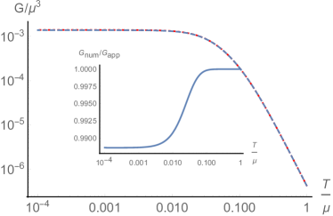
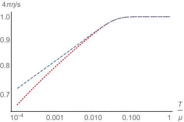
Figure 1: In both plots, the blue dashed curve is the exact numerical result from the Kubo formulæ (10); the red dotted curve is the approximation (46). In the inset, the ratio between the two show a small deviation as temperature decreases. The shear viscosity shows a small sublinear deviation from $s/4\pi$ as $T$ decreases.

The frequency dependence of (37) will only generate $O(\omega^{2})$ corrections which do not contribute to the retarded Green’s function at leading order as $\omega\to 0$. So (42) can be rewritten directly as

$$h_{2}(r)=h^{(reg)}_{2}(r)+i\omega\frac{s}{4\pi}\left(h^{(reg)}_{2}(r_{h})\right)^{2}h^{(sing)}_{2}(r)+O(\omega^{2})\,.$$ (43)

Close to the AdS boundary, $h_{2}^{(reg)}\sim 1+k^{2}I_{Y}r^{3}/3+O(r^{4})$ while $h^{(sing)}_{2}\sim-r^{3}/3+O(r^{4})$, so that the full solution asymptotes to

$$h_{2}(r\to 0)\sim 1+\left(k^{2}I_{Y}-i\omega\frac{s}{4\pi}\left(h^{({reg})}_{2}(r_{h})\right)^{2}\right)\frac{r^{3}}{3}+O(r^{4},\omega^{2})\,.$$ (44)

From this equation, by applying standard holographic formulæ relating the vev of an operator of dimension $3$ in $d=2$ to the asymptotic data of the dual field in the bulk Ammon:2015wua ; Zaanen:2015oix ; Hartnoll:2016apf , we extract the low frequency limit of the shear retarded Green’s function

$$\lim_{\omega\to 0}G^{R}_{T^{xy}T^{xy}}(\omega,\vec{q}=0)=k^{2}I_{Y}-i\omega\frac{s}{4\pi}\left(h^{({reg})}_{2}(r_{h})\right)^{2}\,.$$ (45)

Matching to the hydrodynamic prediction (10), we obtain approximate, small $k$ expressions for the shear modulus and shear viscosity

$$G=k^{2}I_{Y}+O(k^{4})\,,\quad\eta=\frac{s}{4\pi}\left(1-2k^{2}\int_{0}^{r_{h}}dr_{1}\sqrt{\frac{B}{D}}\frac{1}{C}\int^{r_{h}}_{r_{1}}dr_{2}\sqrt{BD}Y+O(k^{4})\right).$$ (46)

They match the exact numerical results very well, see figure 1. We observe in figure 1 that $G$ decreases sharply above $T/\mu\gtrsim 0.1$: at high $T$, the spontaneous component of the system becomes very weak, but never vanishes.

4 Diffusivity matrix from horizon data

In this section, we compute the diffusivities $\sigma_{o}$, $\gamma_{1}$ and $\xi$ in terms of a combination of horizon and UV-sensitive data through a DC analysis, drawing on previous works Donos:2014uba ; Donos:2014cya ; Amoretti:2017frz ; Amoretti:2017axe ; Donos:2018kkm ; Gouteraux:2018wfe . To that end, we turn on the following DC (linear in time) perturbation:

$$\delta a_{x}=a(r)-p_{1}(r)\,t\ ,\quad\delta h_{tx}=h_{1}(r)-p_{2}(r)\,t\ ,\quad\delta h_{rx}=h_{3}(r)\ ,\quad\delta\psi_{x}=\chi(r)-k\,t\delta v.$$ (47)

The mode $\delta v$ corresponds to a vev, and in fact can be set to zero by a Galilean boost Donos:2018kkm ; Gouteraux:2018wfe . It is not fixed by the horizon analysis, and represents the freedom to slide the system back and forth. Upon turning on relaxation, this mode either becomes a source Amoretti:2018tzw or is fixed by the horizon analysis Donos:2019tmo .

All time dependence drops out from the linearized equations, provided

$$p_{1}(r)=p_{1}^{(0)}+\bar{E}\rho A\ ,\qquad p_{2}(r)=-\bar{E}\rho D\ ,$$ (48)

where $p_{1}^{(0)}$ is a constant which will be fixed shortly and $\bar{E}$ a source of the dual field theory to be defined more precisely below.

The following boundary expansions are compatible with the equations of motion:

$$a(r)=a^{(1)}r+O(r^{2})\ ,\quad h_{1}(r)=h_{1}^{(1)}r+O(r^{2})\ ,\quad h_{3}(r)=O(r)\ ,\quad\chi(r)=\frac{\chi_{(0)}}{r}+\chi_{(1)}+O(r)\ ,$$ (49)

provided we set

$$p_{1}^{(0)}=-\bar{E}\left(\frac{9}{2}d_{3}+\rho\mu\right)+\frac{k}{\rho}(\phi_{(v)})^{2}\chi_{0}=\bar{E}\left(sT+k^{2}I_{Y}\right)+\frac{\delta s_{\varphi}}{\rho}.$$ (50)

This condition follows from requesting $\delta h_{rx}$ to fall off sufficiently fast in the UV. It differs from our previous work Amoretti:2017frz by the term proportional to the phonon source $\delta s_{\varphi}=k(\phi_{(v)})^{2}\chi_{(0)}$.

Next, we define two bulk currents:

$$\mathcal{J}(r)=\sqrt{-g}Z(\phi)F^{rx}=Z\sqrt{\frac{D}{B}}a^{\prime}-\rho\frac{h_{1}}{C}\,,\quad\mathcal{Q}(r)=-\sqrt{\frac{D}{B}}h_{1}{}^{\prime}+\frac{D^{\prime}h_{1}}{\sqrt{BD}}-A\mathcal{J}\,,$$ (51)

whose radial evolution is governed by the equations

$$\mathcal{J}^{\prime}=0\,,\qquad\left(\mathcal{Q}+\delta vk^{2}\int_{0}^{r}d\tilde{r}\,\sqrt{DB}Y\right)^{\prime}=0$$ (52)

and which asymptote respectively to the boundary electric and heat currents:

$$j=\mathcal{J}(0)=a^{(1)}\,,\qquad j_{q}\equiv T^{tx}-\mu j=\mathcal{Q}(0)=-3h_{1}^{(1)}-\mu a^{(1)}\,.$$ (53)

Using (52), we can relate the boundary currents to data on the horizon:

$$j=\mathcal{J}(r_{h})\,,\qquad j_{q}=\mathcal{Q}(r_{h})+k^{2}I_{Y}\delta v\,.$$ (54)

Horizon regularity of the solution in ingoing Eddington-Finkelstein coordinates $\textrm{v}=t+1/(4\pi T)\ln(r_{h}-r)+O(r_{h}-r)$ implies that the linear perturbation has the following near-horizon expansion:

$$\begin{split}&a=\left[-\bar{E}\frac{sT+k^{2}I_{Y}}{4\pi T}+\frac{\delta s_{\varphi}}{4\pi T\rho}\right]\log(r_{h}-r)(1+O(r_{h}-r))\ ,\\ &h_{1}=-\bar{E}\frac{\rho I_{Y}}{Y_{h}}-\frac{\delta s_{\varphi}}{k^{2}Y_{h}}-\frac{s}{4\pi}\delta v+O(r_{h}-r)\ ,\\ &h_{3}=-\frac{h_{1}}{4\pi T(r_{h}-r)}+O(1)\ .\end{split}$$ (55)

Evaluating the currents in (54) at the horizon, we find

$$j =\left[(sT+k^{2}I_{Y})Z_{h}+\frac{4\pi\rho^{2}I_{Y}}{sk^{2}Y_{h}}\right]\bar{E}+\left[\frac{4\pi\rho}{sk^{2}Y_{h}}+\frac{Z_{h}}{\rho}\right]\delta s_{\varphi}+\rho\delta v\,,$$ (56)

$$j_{q} =\frac{4\pi T\rho I_{Y}}{Y_{h}}\bar{E}+\frac{4\pi T}{k^{2}Y_{h}}\delta s_{\varphi}+\left(sT+k^{2}I_{Y}\right)\delta v\,.$$ (57)

In order to compute $\sigma_{0}$, $\gamma_{1}$ and $\xi$ we can use the relation between the hydrodynamic correlators (11), (12) and the expectations values of the related current densities, namely:

$$J_{A}=G_{AB}\,S_{B}\,,$$ (58)

with $J_{A}=\{j,j_{q},j_{\varphi}\}$, $S_{A}=\{E_{x}/(i\omega),-\nabla_{x}T/(i\omega T),\delta s_{\varphi}\}$ and where $j_{\varphi}=\dot{\varphi}$ (which can loosely be thought of as the contribution of the phonons to the electric current RevModPhys.60.1129 ). The boundary electric field and temperature gradients are given by the boundary behaviour of the bulk fields:

$$E_{x}=-\lim_{r\to 0}\partial_{t}\left(\delta a_{x}(r,t)+\mu\delta h_{tx}(r,t)\right)\ ,\qquad\frac{1}{T}\nabla_{x}T=\lim_{r\to 0}\partial_{t}\delta h_{tx}(r,t)\,.$$ (59)

By rotating to the basis of currents $(j_{inc}\equiv\chi_{\pi j_{q}}j-\chi_{j\pi}j_{q},\pi)$, $\bar{E}$ can be understood as the source of the incoherent current $j_{inc}$, Amoretti:2017frz . The incoherent current is the part of the electric current which does not drag momentum, Davison:2015taa . In other terms, $\chi_{j_{inc}\pi}=0$.

Using (48) and (50), the electric field and temperature gradient can be expressed in terms of the sources $\bar{E}$ and $\delta s_{\phi}$:

$$E_{x}=(\chi_{\pi\pi}-\mu\rho)\bar{E}+\frac{\delta s_{\varphi}}{\rho}\ ,\qquad\nabla_{x}T=\bar{E}\rho T\,,$$ (60)

where $\chi_{\pi\pi}$ is given by (32). We can now form the following linear combination of currents and relate them to the sources we have turned on using the hydrodynamic correlators (11), (12):

$$\chi_{\pi j_{q}}j-\chi_{j\pi}j_{q} =\chi_{\pi\pi}^{2}\sigma_{0}\bar{E}+\chi_{\pi\pi}\left(\frac{\sigma_{0}}{\rho}-\gamma_{1}\right)\delta s_{\varphi}\,,$$ (61)

$$\mu j+j_{q}+\chi_{\pi\pi}j_{\varphi} =-\bar{E}\gamma_{1}\chi_{\pi\pi}^{2}+\delta s_{\varphi}\chi_{\pi\pi}\left(X-\frac{\gamma_{1}}{\rho}\right)\,,$$ (62)

where $\chi_{\pi j_{q}}=\chi_{\pi\pi}-\mu\rho$. This follows from $j_{q}=\pi-\mu j$, as required by relativistic symmetry. Undoing the term $\delta v$ in $\delta\psi_{x}$ with a Galilean boost amounts to shifting the currents $j$, $j_{q}$ by terms proportional to $\delta v$. These terms can in turn be absorbed by a redefinition of the velocity $v^{x}$, which finally gives a contribution to $j_{\varphi}=-\delta v$, recalling the Josephson relations (2). Substituting (56) and (57) on the left hand side of (61) and (62), we find that

$$\sigma_{0} = \frac{\left(sT+k^{2}I_{Y}\right)^{2}}{\left(sT+\mu\rho+k^{2}I_{Y}\right)^{2}}Z_{h}+\frac{4\pi k^{2}(I_{Y})^{2}\rho^{2}}{sY_{h}\left(sT+\mu\rho+k^{2}I_{Y}\right)^{2}}\,,$$ (63)

$$\gamma_{1} = -\frac{4\pi I_{Y}\rho\left(sT+\mu\rho\right)}{sY_{h}\left(sT+\mu\rho+k^{2}I_{Y}\right)^{2}}-\mu\frac{\left(sT+k^{2}I_{Y}\right)}{\left(sT+\mu\rho+k^{2}I_{Y}\right)^{2}}Z_{h}\,,$$ (64)

$$X = \frac{4\pi\left(sT+\mu\rho\right)^{2}}{k^{2}sY_{h}\left(sT+\mu\rho+k^{2}I_{Y}\right)^{2}}+\frac{\mu^{2}Z_{h}}{\left(sT+\mu\rho+k^{2}I_{Y}\right)^{2}}\,,$$ (65)

where we have used (32) for $\chi_{\pi\pi}$. The dependence on UV-sensitive data is manifest through factors of $\mu$ and $I_{Y}$.

As we already commented upon at the end of section 3.3, the expressions (63)-(65) give an excellent match to the zero frequency limit of the ac correlators.

5 Saturation of entropy bound and universal relaxation

WC hydrodynamics predicts a bound coming from positivity of entropy production Delacretaz:2017zxd ,

$$\gamma_{1}^{2}\leq\sigma_{o}X\,,$$ (66)

which is obeyed by our DC expressions for the diffusivities:

$$\sigma_{0}X-\gamma_{1}^{2}=\frac{4\pi sT^{2}Z_{h}}{k^{2}(\chi_{\pi\pi})^{2}Y_{h}}\geq 0\,.$$ (67)

See figure 2.

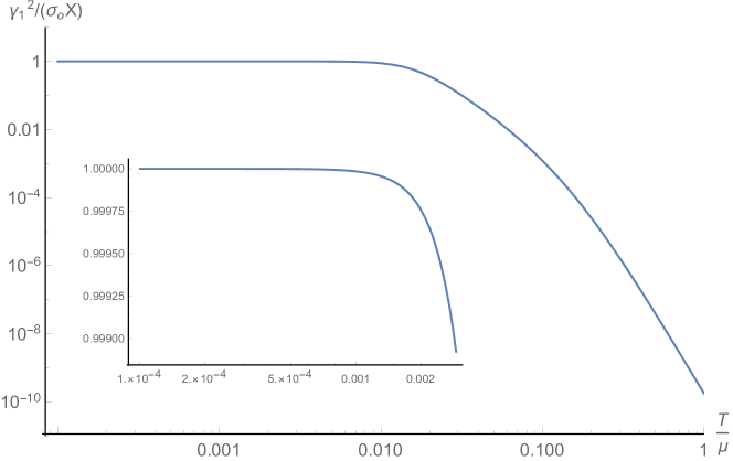
Figure 2: At all temperatures, the entropy bound $\gamma_{1}^{2}\leq\sigma_{o}X$ holds. At low temperatures, the bound is saturated.

Interestingly, for our specific choice of holographic model, the bound becomes saturated at low temperatures. Indeed, for the $z=+\infty$, $\theta=-\infty$, $-\theta/z=1$ family we have mostly focussed on, $Z_{h}\sim 1/T$, $Y_{h}\sim T^{0}$ and $s\sim T$. Saturation of (66) relates the diffusivities $\sigma_{o}$, $X$ and $\gamma_{1}$ to one another. This is reminiscent of the relation between second-order transport coefficients of fluid hydrodynamics uncovered in Haack:2008xx . Magnetohydrodynamics is another example where a bound originating from the positivity of entropy production Grozdanov:2016tdf is saturated in an explicit holographic realization Grozdanov:2017kyl .

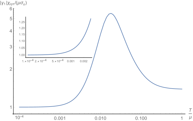
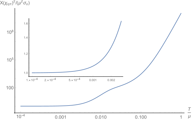
Figure 3: At low temperatures, the entropy bound is saturated and the diffusivities $\gamma_{1}$, $X$ are controlled by the thermal diffusivity through (73).

To understand this feature, we consider the following Kubo formulæ for the diffusivities:

$$\gamma_{1} = -\lim_{\omega\to 0}\frac{1}{\omega}\textrm{Im}G^{R}_{j\dot{\varphi}}(\omega,q=0)\,,$$ (68)

$$X = \lim_{\omega\to 0}\frac{1}{\omega}\textrm{Im}G^{R}_{\dot{\varphi}\dot{\varphi}}(\omega,q=0)\,,$$ (69)

$$\sigma_{o} = \lim_{\omega\to 0}\frac{1}{\omega}\textrm{Im}G^{R}_{jj}(\omega,q=0)\,.$$ (70)

The Kubo formulæ (68), (69) involve the operator $\dot{\varphi}$, which suggests that a memory-matrix type analysis should apply Delacretaz:2019 . Relaxation of the Goldstones into the heat current provides a particularly appealing and universal mechanism for systems at finite temperature. It contributes to the low energy Hamiltonian via a term

$$\Delta\mathcal{H}=\frac{1}{\chi_{\pi j_{q}}}\pi\cdot j_{q}\,.$$ (71)

The full Hamiltonian will contain other contributions from non-hydrodynamic operators. Here we assume these other terms do not dominate at low temperatures. The contribution from (71) to $\dot{\varphi}$ is

$$\dot{\varphi}=i[\Delta\mathcal{H},\varphi]=\frac{j_{q}}{\chi_{\pi j_{q}}}\,.$$ (72)

This equation shows that the time evolution of the Goldstone operator is governed by the heat current, as advertised. Plugging this in the Kubo formulæ above relates the diffusivities $\gamma_{1}$, $\xi$ to the thermal diffusivity:

$$\gamma_{2}=-\frac{\mu}{T}\gamma_{1}=\frac{\mu^{2}}{T\chi_{\pi j_{q}}}\sigma_{o}=\frac{\bar{\kappa}_{o}}{\chi_{\pi j_{q}}}\,,\qquad X=\left(\frac{\mu}{\chi_{\pi j_{q}}}\right)^{2}\sigma_{o}=\frac{T}{\chi_{\pi j_{q}}^{2}}\bar{\kappa}_{o}\,,$$ (73)

where we have also used (7). For the $\theta=-\infty$, $z=+\infty$, $\theta/z=-1$ state we have considered in detail in this work, these expressions capture the correct low temperature behaviour of the diffusivities (see figure 3), and lead to the saturation of the entropy bound (66). At higher temperatures, other, non-universal relaxation channels will open. For the $\theta=-\infty$, $z=+\infty$, $\theta/z=-1$ holographic state, these non-hydrodynamic operators also contribute to the Hamiltonian (71) but give subleading corrections as $T\to 0$.

It is interesting to assess how generic the universal relaxation mechanism we have just described is. To do so, we consider the more general family of IR end points (24). It is clear that if there is no running scalar $\phi$ and the IR is AdS${}_{2}\times$R², the entropy bound is saturated since all factors in (67) scale like $T^{0}$ at low temperatures, except of course for the explicit $T^{2}$ factor. When there is a running scalar, there are four classes of IR end points, characterized by the presence or absence of certain dangerously irrelevant deformations. These are discussed in some detail in Gouteraux:2014hca ; Amoretti:2017frz ; Amoretti:2017axe and more recently in Davison:2018nxm , so we will be brief here.

There are two potentially dangerously irrelevant deformations, depending on whether the bulk fields dual to the conserved current and dual to the phonons support the deep IR solution or whether they decay faster than other fields in the bulk. These deformations can be usefully characterized by the scaling dimension of the coupling, which we denote by $\Delta_{A_{o}}$ and $\Delta_{k}$, respectively. In order for the coupling to source an irrelevant/marginal deformation, $\Delta_{A_{o},k}\leq 0$. The four classes differ by whether both deformations are marginal, or only one of them is, or both of them are irrelevant. In the case we have studied numerically and for which the bound is saturated, both deformations are marginal $\Delta_{A_{o}}=\Delta_{k}=0$. Their expressions in terms of the action couplings have been given in (25)

Evaluating the right-hand side of (67) on the solutions (24) together with the expressions (23), (25) for the IR couplings and recalling that $s\sim T^{(d-\theta)/z}$, the entropy bound is saturated provided

$$\frac{2}{z}\left(z-2+\Delta_{A_{o}}+\Delta_{k}\right)\geq 0\,.$$ (74)

We find that this condition is met provided

$$z>2\quad\textrm{and}\quad\theta<2\quad\textrm{and}\quad 2-z<\Delta_{A_{o},k}\leq 0\,.$$ (75)

In particular, this implies the bound is never saturated for IR end points with relativistic symmetry $z=1$, which only happens when both deformations are irrelevant. If only one deformation is irrelevant, then the dimension of the coupling is bounded from below. If both are marginal $\Delta_{A_{o},k}=0$, then the bound is saturated if the dynamical exponent $z$ is large enough, $z>2$.

In the parameter space spanned by (75), we observe that $(2+z-\theta)>-\Delta_{A_{o},k}$. Recalling that $sT\sim T^{(2+z-\theta)/z}$ at low temperature, this suggests that $sT$ terms can be neglected at low temperatures in (63)-(65) against other terms that have a non-vanishing zero temperature limit, such as $\mu\rho$ or $k^{2}I_{Y}$. Doing so leads to

$$\sigma_{0} = \frac{\left(k^{2}I_{Y}\right)^{2}}{\left(\mu\rho+k^{2}I_{Y}\right)^{2}}\left(Z_{h}+\frac{4\pi\rho^{2}}{sk^{2}Y_{h}}\right),$$ (76)

$$\gamma_{1} = -\frac{\mu k^{2}I_{Y}}{\left(\mu\rho+k^{2}I_{Y}\right)^{2}}\left(Z_{h}+\frac{4\pi\rho^{2}}{sk^{2}Y_{h}}\right),$$ (77)

$$X = \frac{\mu^{2}}{\left(\mu\rho+k^{2}I_{Y}\right)^{2}}\left(Z_{h}+\frac{4\pi\rho^{2}}{k^{2}sY_{h}}\right).$$ (78)

We have verified that these expressions are consistent with our numerics at low temperature. It is straightforward to check that the expressions (76)-(78) saturate the entropy bound (66).

The prefactors are all temperature independent at low $T$, so all the low temperature dependence comes from the common factor in parenthesis. Since this common factor is the same for all three quantities, the saturation of the bound comes from the cancelation between the prefactors in the limit of low temperature, rather than from the vanishing of each individual term in (66).

On the other hand, requiring $(2+z-\theta)>-\Delta_{A_{o},k}$ does not imply that the entropy bound is saturated. It would be interesting to further investigate these cases and to understand why the universal mechanism (71) is not at play there.

6 Transverse collective excitations at nonzero wavevector

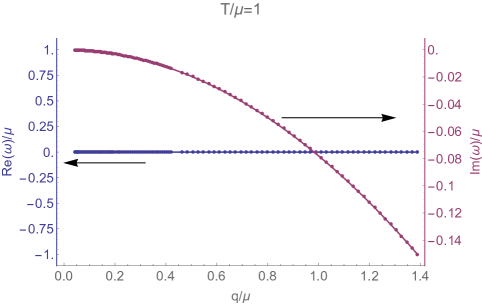
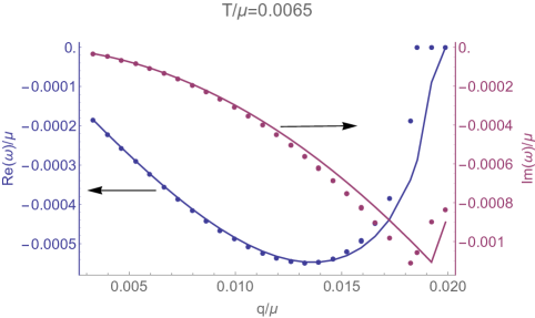
Figure 4: Comparison of the exact location (dots, numerics) and hydrodynamic approximation (79) (solid lines) of the real (blue, left axis) and imaginary (magenta, right axis) part of the transverse hydrodynamic QNM at $T/\mu=1$ (top), $T/\mu=0.1$ (center) and $T/\mu=0.0065$ (bottom) vs $q/\mu$. In the top panel, the modes are purely imaginary, but would acquire a real part at smaller $q$ (not displayed).

WC hydrodynamics also predicts the existence of a pair of low energy modes in the transverse channel. They appear as zeroes of the denominator of the hydrodynamic retarded Green’s functions and their dispersion relation is:

$$\omega_{shear}=\frac{1}{2}\left[-iq^{2}\left(\xi_{\perp}+\frac{\eta}{\chi_{\pi\pi}}\right)\pm q\sqrt{4\frac{G}{\chi_{\pi\pi}}-q^{2}\left(\frac{\eta}{\chi_{\pi\pi}}-\xi_{\perp}\right)^{2}}\right].$$ (79)

At sufficiently low wavector $q$, these modes are gapless and propagate transverse sound waves:

$$\omega_{shear}=\pm\sqrt{\frac{G}{\chi_{\pi\pi}}}\,q-\frac{i}{2}q^{2}\left(\xi_{\perp}+\frac{\eta}{\chi_{\pi\pi}}\right)+O(q^{3})\,.$$ (80)

On the other hand, for larger values of $q>2\sqrt{G\chi_{\pi\pi}}/(\eta-\xi_{\perp}\chi_{\pi\pi})$, the modes collide on the imaginary axis and are no longer propagating. Instead, they obey a pseudo-diffusive dispersion relation:

$$\omega_{-}=-i\xi_{\perp}q^{2}-\frac{iG}{\eta-\xi_{\perp}\chi_{\pi\pi}}+O(q^{-1})\,,\quad\omega_{+}=-i\frac{\eta}{\chi_{\pi\pi}}q^{2}+\frac{iG}{\eta-\xi_{\perp}\chi_{\pi\pi}}+O(q^{-1})\,.$$ (81)

Observe that while the sign of the $q^{0}$ damping term is positive for one of the modes, this does not lead to an instability since $q$ is large. This collision is captured by the hydrodynamic dispersion relation, since the inequality on $q$ is true if $G$ is small enough. We expect $G$ to be small also close to a phase transition between a translationally ordered and a translationally disordered phase.

We compare the exact location of the quasinormal modes determined numerically to the hydrodynamic approximation in figure 4 as a function of $q/\mu$, and find they agree very well, including at very low temperatures. We typically observe deviations when $q\gtrsim T$, which suggests that temperature is the cut-off of the effective description in terms of WC hydrodynamics, whether $T$ is large or small compared to the chemical potential $\mu$. This gives strong evidence that the low energy excitations of our system are well described by WC hydrodynamics at all temperatures, and further confirms that our holographic model should be interpreted as describing the low energy dynamics of (pseudo)phonons coupled to conserved currents. We emphasize that the same dispersion relation is valid at both low and high temperature. Similar results on the low-temperature hydrodynamics of translation-invariant black holes have been reported in past literature Edalati:2010hk ; Edalati:2010pn ; Davison:2013bxa .

Figure 5: Comparison of the exact location (numerics, solid blue) and hydrodynamic approximation (79) (dashed, red) of the real (inset) and imaginary part of the transverse hydrodynamic QNM at $q/\mu=0.02$ vs $T/\mu$. At intermediate temperatures, they follow very well the dispersion relation of shear sound waves predicted by WC hydrodynamics. At both very high and very low $T$, the modes collide and become purely imaginary and pseudo-diffusive. Keeping $T/\mu$ fixed, they modes acquire a nonzero real part as $q$ is lowered, see figure 4.

In figure 5, we display the QNMs location as a function of $T/\mu$ and compare it to (79). Increasing temperature, the shear sound modes collide on the imaginary axis. At these temperatures, the shear modulus of the system becomes very small (see figure 1), and this is the underlying reason behind the high temperature pole collision (see figure 5). The same loss of shear rigidity would occur in a real crystal right before the phase transition to a liquid phase: the solid would no longer support gapless, transverse sound modes. The two high temperature branches are well-approximated by (81), with $\omega_{+}$ giving the longest-lived mode. In other words, as the spontaneous component of the system is becoming very small, the system resembles more and more a fluid (consistently with the gap of (81) being proportional to $G$, which is going to zero as $T\to+\infty$).

At low temperatures, the QNMs also undergo a collision, which is now driven by the fact that $\xi_{\perp}\sim 1/T$ is becoming very large. Once again, the longest-lived mode is well-approximated by $\omega_{+}$ in (81). The gap is inversely proportional to $\xi_{\perp}$ and decreases with $T$, see figure 6. The system resembles more and more a fluid since the phonons relax faster (they have a larger diffusivity).

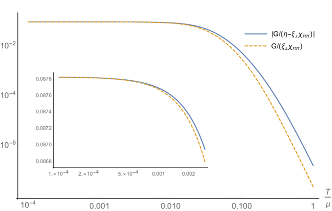
Figure 6: At low temperatures, the gap at large wavevector is dominated by the phonon diffusivity $\xi_{\perp}$ rather than by the shear viscosity $\eta$.

Similar collisions between high temperature, gapped, pseudo-diffusive modes leading to low temperature propagating modes have been reported in previous holographic literature Davison:2014lua ; Grozdanov:2018ewh ; Baggioli:2018vfc ; Grozdanov:2018fic . There are important differences. In our case, translations are broken spontaneously, not explicitly. As a consequence, at the longest distances $q\to 0$, the modes are always gapless, sound modes. The collision we report is ‘coherent’ or in other words, can be described by a hydrodynamic effective theory (WC hydrodynamics). In contrast, in Davison:2014lua ; Baggioli:2018vfc ; Grozdanov:2018fic the breaking is always explicit and the effective theory is momentum-relaxed fluid hydrodynamics, and breaks down below a certain temperature where momentum is no longer approximately long-lived. In Grozdanov:2018ewh , translations are broken spontaneously, but the transverse propagating modes are gapped. Gapless propagating modes are found for a nonzero density of defects, and it would be interesting if they became gapped at shorter distances, while remaining within the regime of validity of the hydrodynamic description.

Recently, Ammon:2019wci have also reported similar collisions in a holographic massive gravity model.

7 Outlook

The main results we have obtained are as follows. Firstly, we have shown that all of the diffusivities that characterize the low energy dynamics of a holographic state breaking translations spontaneously can be computed in terms of a combination of horizon and UV-sensitive data. We have focussed on a specific model breaking translations homogeneously, and it would be natural to extend this computation to inhomogeneous, more realistic setups. Moreover, in Donos:2018kkm ; Amoretti:2017frz ; Amoretti:2017axe ; Gouteraux:2018wfe , the incoherent conductivity was computed for thermodynamically stable phases and solely depends on horizon data.

We have also shown how the low temperature behaviour of these diffusivities and the saturation of an entropy bound stemming from Wigner crystal hydrodynamics is explained by the universal relaxation of the phonons into the heat current. We have studied whether this depends on the infra-red end point controlling the system at zero temperature. We found that the entropy bound is not saturated in the presence of sufficiently irrelevant deformations, or for values of the dynamical exponent $1\leq z\leq 2$.

Finally, we have studied the spectrum of transverse collective excitations and discovered that for sufficiently low wavectors the pair of longest-lived modes are well captured by the dispersion relation following from WC hydrodynamics, including at low temperatures where the system is governed by the IR end point consistent with previous low temperature holographic studies Edalati:2010hk ; Edalati:2010pn ; Davison:2013bxa . We observed deviations as $q\gtrsim T$. In particular, this means that the hydrodynamic description extends outside of the regime $q\ll T$ to $q\simeq T$ where gradients are of the same order as the thermal scale. This ‘unreasonable effectiveness’ of hydrodynamics could perhaps be understood along the lines of the recent work Grozdanov:2019kge .

We have only carried out explicit numerical calculations for the special case $z=-\theta=+\infty$. As we have observed, the saturation of the entropy bound will not occur for phases with $z\leq 2$, in particular for $z=1$ in the presence of irrelevant deformations. It was shown in Davison:2018ofp ; Davison:2018nxm that in these cases new long-lived modes emerge at low temperature and lead to a breakdown of the hydrodynamic description at earlier times than that set by temperature. A natural future direction would be to study these cases with spontaneous translation symmetry breaking.

If translations are explicitly broken, the phonons obtain a mass $m$ and are damped, with a phase relaxation rate $\Omega$ (this phase relaxation rate is of a different microscopic origin than the phase relaxation rate sourced by the proliferation of topological defects PhysRevLett.41.121 but appears in the effective theory in exactly the same way). WC hydrodynamics in the presence of relaxation also predicts a bound on the relaxation parameters Delacretaz:2017zxd

$$\gamma_{1}^{2}\leq\textrm{min}\left(\sigma_{o}X,\frac{\sigma_{o}\Omega}{Gm^{2}}\right).$$ (82)

In Amoretti:2018tzw , we showed that turning on a small source for the scalar $\phi$ in our holographic model led to a phase whose low energy effective theory was relaxed WC hydrodynamics, until very low temperatures. The bound (82) is also saturating as temperature decreases, suggesting that the pseudo-phonons also relax universally into the heat current. It would be interesting to understand how this depends on the infra-red end point, the relaxation mechanism and the details of how translations are broken in the holographic model. By now, many other models of pinned translational order are available Jokela:2017ltu ; Alberte:2017cch ; Andrade:2017cnc ; Andrade:2017ghg ; Andrade:2018 ; Donos:2019tmo ; Ammon:2019wci .

In the presence of a magnetic field, the longitudinal and transverse phonons hybridize into a magnetophonon and a magnetoplasmon PhysRevB.18.6245 . For strong magnetic fields and in the presence of disorder, the magnetophonon is weakly gapped and a hydrodynamic theory can be formulated Delacretaz:2019 , which appears to fit well some of the data on two-dimensional electron systems. Universal relaxation of the magnetophonon into the electric current may dominate (compared to dislocation-mediated melting) in more disordered samples, and it would be interesting to study this holographically (see Romero-Bermudez:2019lzz for a recent study of plasmonic response at zero field in the holographic model studied here).

Appendix A AC boundary correlators at zero density

First, we need to figure out how to extract the retarded Green’s functions (12) from the asymptotic data. The relevant part of the renormalized on-shell action at quadratic order in the fluctuations (34) (keeping only $h_{1,(0)}$ and $\delta\psi_{(-1)}$ nonzero) is

$$S_{\rm ren}^{(2)}=\left.\int d\omega\left[-\frac{3}{2}\delta h_{1,(0)}\delta h_{1,(3)}+\frac{3}{2}d_{(3)}(\delta h_{1,(0)})^{2}+(\phi_{(v)})^{2}\delta\psi_{(-1)}\delta\psi_{(0)}\right]\right|_{\delta a_{(0)},\delta h_{2,(0)}=0}$$ (83)

so that the retarded Green’s function are

$$\begin{split}G^{R}_{T^{tx}T^{tx}}(\omega,q=0)=\frac{3\delta h_{1,(3)}}{\delta h_{1,(0)}}\,,&\quad G^{R}_{T^{tx}\delta\psi_{x}}(\omega,q=0)=\frac{3\delta h_{1,(3)}}{\delta\psi_{(-1)}}\,,\\ G^{R}_{\delta\psi_{x}T^{tx}}(\omega,q=0)=(\phi_{(v)})^{2}\frac{\delta\psi_{(0)}}{\delta h_{1,(0)}}\,,\quad&G^{R}_{\delta\psi_{x}\delta\psi_{x}}(\omega,q=0)=(\phi_{(v)})^{2}\frac{\delta\psi_{(0)}}{\delta\psi_{(-1)}}\,.\end{split}$$ (84)

We start by explicitly identifying the source of the boundary phonon. This is done by plugging the UV expansions (33) for the bulk fluctuations and solving the equations of motion, which give the following relation

$$\delta h_{1,(3)}=\frac{i}{\omega}\frac{k(\phi_{(v)})^{2}\delta\psi_{(-1)}}{3}$$ (85)

from which we immediately deduce

$$G^{R}_{T^{tx}\delta\psi_{x}}(\omega,q=0)=\frac{3\delta h_{1,(3)}}{\delta\psi_{(-1)}}=k(\phi_{(v)})^{2}\frac{i}{\omega}\,.$$ (86)

In order for this expression to match the off-diagonal Green’s function $G^{R}_{\pi\varphi}$ in (12), we see that we should identify the phonon source as $\delta s=k(\phi_{(v)})^{2}\delta\psi_{(-1)}$.

To continue, we now need to solve the equations of motion away from the boundary. It is helpful to define the variable Davison:2018nxm

$$\Pi_{x}\equiv-\frac{{h^{x}_{t}}^{\prime}+i\omega h^{x}_{r}}{\left(D/C\right)^{\prime}}\,,$$ (87)

which obeys the decoupled equation of motion

$$\frac{d}{dr}\left[\sqrt{\frac{D}{B}}\frac{1}{YC}\left(\frac{C^{2}}{\sqrt{BD}}\left(\frac{D}{C}\right)^{\prime}\right)^{2}\Pi_{x}^{\prime}\right]+\omega^{2}\sqrt{\frac{B}{D}}\frac{1}{YC^{2}}\left(\frac{C^{d/2+1}}{\sqrt{BD}}\left(\frac{D}{C}\right)^{\prime}\right)^{2}\Pi_{x}=0.$$ (88)

Then we can expand $\Pi_{x}$ in $\omega$

$$\Pi_{x}(r)=\left(sT+k^{2}\int^{r_{h}}_{r}\sqrt{BD}Y\right)\left(1-\frac{r}{r_{h}}\right)^{-i\omega/(4\pi T)}\left(\pi_{o}+\frac{i\omega}{4\pi T}\pi_{1}(r)+\dots\right)$$ (89)

and solve order by order, imposing ingoing boundary conditions. At leading order, $\pi_{o}$ is just a constant. The solution for $\pi_{1}$ which is regular at the horizon is

$$\pi_{1}(r)=i\pi_{o}\int_{r_{h}}^{r}dr_{1}\left[\frac{1}{r_{1}-r_{h}}+(4\pi T)^{3}\frac{C_{h}}{Y_{h}}\frac{\sqrt{B}CY}{\sqrt{D}\left(sT+k^{2}\int^{r_{h}}_{r_{1}}\sqrt{BD}Y\right)^{2}}\right].$$ (90)

To go through these manipulations, it is helpful to keep in mind the relation (31):

$$\frac{C^{2}}{\sqrt{BD}}\left(\frac{D}{C}\right)^{\prime}=-sT-k^{2}\int^{r_{h}}_{r}\sqrt{BD}Y.$$ (91)

The boundary expansion of the $\Pi_{x}$ variable is

$$\Pi_{x}=\frac{i}{\omega}k(\phi_{(v)})^{2}\delta\psi_{(-1)}+\frac{i\omega}{2}k(\phi_{(v)})^{2}\delta\psi_{(-1)}r^{2}+\frac{1}{3}k(\phi_{(v)})^{2}\left(k\delta h_{1,(0)}+i\omega\delta\psi_{(0)}\right)r^{3}+\dots$$ (92)

To establish this, it is necessary to push the boundary expansions to higher order in $r$ than written in (33). Also, we note that the combination that appears at $O(r^{3})$ is gauge invariant. So from (84) the retarded Green’s function for $\delta\psi_{x}$ is

$$G^{R}_{\delta\psi_{x}\delta\psi_{x}}(\omega,q=0)=\frac{(\phi_{(v)})^{2}}{2\omega^{2}}\lim_{r\to 0}\frac{\Pi_{x}^{(3)}(r)}{\Pi_{x}(r)}\,.$$ (93)

Putting together (89) and (90), we obtain after expanding at low frequency

$$G^{R}_{\delta\psi_{x}\delta\psi_{x}}(\omega,q=0)=\left(k(\phi_{(v)})^{2}\right)\left[\frac{1}{\left(\frac{9}{2}d_{(3)}\right)\omega^{2}}+\frac{4\pi sT^{2}}{k^{2}Y_{h}\left(\frac{9}{2}d_{(3)}\right)^{2}}\frac{i}{\omega}\right]$$ (94)

The momentum static susceptibility was computed in Amoretti:2017frz

$$\chi_{\pi\pi}=-\frac{9}{2}d_{(3)}=sT+k^{2}\int_{r_{h}}^{0}\sqrt{BD}Y\,.$$ (95)

Observe that our boundary expansions imply that the integral over the whole bulk does not diverge at the boundary. Plugging into (94) and comparing with the phonon retarded Green’s function $G^{R}_{\varphi\varphi}$ in (12) leads to identifying the phonon as

$$\varphi_{x}=\frac{\delta\psi_{(0)}}{k(\phi_{(v)})^{2}}$$ (96)

and the ratio of the transverse crystal diffusivity to the shear modulus as

$$\frac{\xi_{\perp}}{G}=\frac{4\pi sT^{2}}{k^{2}Y_{h}\left(sT+k^{2}\int_{0}^{r_{h}}\sqrt{BD}Y\right)^{2}}\,.$$ (97)

This result matches the zero density limit of (65).

Appendix B Numerics

In this appendix we describe how we construct the numerical solutions of the holographic model (16) relevant for the analysis presented in the main text.

B.1 Black hole geometries

The action (16) admits black hole solutions asymptotic to AdS which realize holographically the (pseudo-)spontaneous breaking of translations. In order to find those geometries we take the following Ansatz for the metric and matter fields

$$ds^{2}={1\over r^{2}}\left(-u(r)dt^{2}+{1\over u(r)}dr^{2}+c(r)(dx^{2}+dy^{2})\right)\,,$$ (98)

$$A=A_{t}(r)dt\,,\quad\phi=\phi(r)\,,\quad\psi_{I}=kx^{I}\,,\quad x^{I}=\{x,y\}.$$ (99)

The resulting equations of motion can be reduced to a system of four ordinary differential equations (three are second order and one is first order). For the potentials in eq. (26) it is easy to find the following UV asymptotic solution:

$$\phi(r)=\lambda\,r+v\,r^{2}+\lambda\left(k^{2}+{7\over 36}\lambda^{2}\right)\,r^{3}+O(r^{4})\,,$$ (100a)

$$A_{t}(r)=\mu-\rho\,r-{\lambda\,\rho\over 2\sqrt{3}}r^{2}-{\rho\over 36}\left(5\lambda^{2}+4\sqrt{3}\,v\right)\,r^{3}+O(r^{4})\,,$$ (100b)

$$u(r)=1-{\lambda^{2}\over 4}\,r^{2}+u_{3}\,r^{3}+O(r^{4})\,,$$ (100c)

$$c(r)=1-{\lambda^{2}\over 4}\,r^{2}-{1\over 3}\lambda\,v\,r^{3}+O(r^{4})\,,$$ (100d)

where higher order coefficients are functions of $\lambda$, $v$, $\rho$, and $u_{3}$. This is not the most general asymptotic solution, but that with AdS asymptotics.

In the IR one can find the following near-horizon solution

$$\phi(r)=\phi_{h}+O(r_{h}-r)\,,\qquad\qquad A_{t}(r)=A_{h,1}(r_{h}-r)+O((r_{h}-r)^{2})\,,$$ (101a)

$$u(r)=u_{h,1}(r_{h}-r)+O((r_{h}-r)^{3})\,,\quad c(r)=c_{h}+c_{h,1}(r_{h}-r)+O((r_{h}-r)^{2})\,,$$ (101b)

where, for the potentials (26)

$$u_{h,1}={c_{h}\,e^{-{\phi_{h}\over\sqrt{3}}}\left[6+e^{2\phi_{h}\over\sqrt{3}}(6-r_{h}^{4}\,A_{h,1})\right]-2k^{2}r_{h}^{2}\left(1-e^{\phi_{h}}\right)^{2}\over 2r_{h}\left(2c_{h}+c_{h,1}\,r_{h}\right)}$$ (102)

determines the temperature of the black hole $T=-u_{h,1}/(4\pi)$, and further higher order coefficients in (101) are also determined in terms of $\phi_{h}$, $A_{h,1}$, $c_{h}$, and $c_{h,1}$.

It is easy to check that the equations of motion enjoy the scale invariance $(t,x,y,r)\to\alpha\,(t,x,y,r)$, $A_{t}\to A_{t}/\alpha$, $k\to k/\alpha$ which we use to set the horizon radius $r_{h}=1$ in our numerical computations. Next we generate numerical solutions by integrating the equations of motion from the IR ($r=1$) to the UV ($r=0$). However, a generic solution obtained this way will not have the UV asymptotics (100). In particular $c(r)=c_{0}+c_{1}\,r+\dots$, and one would need to shoot for $c_{0}=1$, and $c_{1}=0$ to get the AdS asymptotics (100). But one can make use of a further invariance of the equations under $(x,y)\to\beta\,(x,y)$, $k\to k/\beta$, $c\to c/\beta^{2}$ to get $c_{0}=1$. This in practice means that $c_{h}$ is fixed and we are thus left with three IR parameters $\phi_{h}$, $A_{h,1}$, $c_{h,1}$; and one UV condition: $c_{1}=0$. Therefore, we expect to obtain a two-parameter family of solutions. We can choose those parameters to be the dimensionless ratios $T/\mu$ and $\lambda/\mu$.

In this work we are interested in solutions breaking translations spontaneously. These are geometries where $\lambda/\mu$ vanishes but $v/\mu^{2}$ does not (solutions with a nontrivial $\phi$ that behaves asymptotically as $\phi\sim v\,r^{2}+\dots$). As was shown in Amoretti:2017frz , for the choice of potentials (26) these solutions exist for any value of $T/\mu$. In the following we will only consider geometries with $\lambda/\mu=0$.

B.2 AC Fluctuations

In order to compute the boundary correlators analyzed in section 3.3 we consider the following consistent set of fluctuations

$$\delta g_{tx}=h(r)\,e^{-i\omega t}\,,\quad\delta A_{x}=a(r)\,e^{-i\omega t}\,,\quad\delta\psi_{x}=\xi(r)\,e^{-i\omega t}\,.$$ (103)

It is easy to check that at linear order in the fluctuations, the equations of motion for $a$, $h$, and $\xi$ are a consistent set formed by two second order and one first order differential equation.

For a spontaneous background geometry (where $\lambda=0$) the asymptotic UV solution for the fluctuations at hand takes the form

$$h(r)=r^{-2}\left(h_{0}+O(r^{3})\right)\,,$$ (104a)

$$a(r)=a_{0}+a_{1}\,r+O(r^{2})\,,$$ (104b)

$$\xi(r)=\xi_{-1}/r+\xi_{0}+O(r)\,,$$ (104c)

where higher order coefficients are functions of $h_{0}$, $a_{0}$, $a_{1}$, $\xi_{-1}$ and $\xi_{0}$. We shall also write down here the solution for the order $r^{3}$ contribution to $h(r)$ since it will be used below in the computation of the holographic Green functions:

$$h_{3}={\rho\over 3}\,a_{0}+{ik\over 3\omega}\,v^{2}\,\xi_{-1}\,.$$ (105)

We are interested in computing retarded propagators, hence we must require the solutions to be ingoing towards the black hole horizon. They take the form

$$h(r)\,e^{i{\omega\over u_{h,1}}}=h_{h,1}\,(r_{h}-r)+O((r_{h}-r)^{2})\,,$$ (106a)

$$a(r)\,e^{i{\omega\over u_{h,1}}}=a_{h}+O(r_{h}-r)\,,$$ (106b)

$$\xi(r)\,e^{i{\omega\over u_{h,1}}}=\xi_{h}+O(r_{h}-r)\,,$$ (106c)

with

$$h_{h,1}={a_{h}\,A_{h,1}\,e^{-{\phi_{h}\over\sqrt{3}}}\,r_{h}^{2}-\left(e^{\phi_{h}}-1\right)^{2}\xi_{h}\,k/r_{h}\over i\omega/u_{h,1}-1}\,,$$ (107)

and other higher order coefficients determined as well in terms of $a_{h}$, and $\xi_{h}$.

As it will be useful below, let us also point out that the following field configuration

$$h(r)=-i\omega\,{c(r)\over r^{2}}\,,\quad a(r)=0\,,\quad\xi(r)=k\,,$$ (108)

solves the equations of motion, since it results from a diffeomorphism transformation of the trivial solution.

B.2.1 Computing the correlators

We follow Kaminski:2009dh and compute the holographic Green function $G^{R}_{AB}$ where $A,B=h,a,\xi$, as

$$G^{R}_{AB}={\cal B}+{\cal A}\,.\,V\,.\,S^{-1}\,.$$ (109)

The matrices ${\cal A}$ and ${\cal B}$ can be read from the quadratic action for the fluctuations as

$$S_{os}^{(2)}=\int d\omega\left(A_{IJ}\,{\mathfrak{v}}^{J}\,{\mathfrak{s}}^{I}+B_{IJ}\,{\mathfrak{s}}^{J}\,{\mathfrak{s}}^{I}\right),$$ (110)

where ${\mathfrak{s}}$ and ${\mathfrak{v}}$ are vectors made of the leading (sources) and subleading (vevs) coefficients of the bulk fields that in the case at hand read

$${\mathfrak{s}}=(h_{0},a_{0},\xi_{-1})\,,\quad{\mathfrak{v}}=(h_{3},a_{1},\xi_{0})\,.$$ (111)

Therefore, rewriting the quadratic on-shell action (34) in the gauge (98,103) one gets

$${\cal A}=\left(\begin{array}[]{ccc}-3&0&0\\ 0&1&0\\ 0&0&v^{2}\end{array}\right)\,,\quad{\cal B}=\left(\begin{array}[]{ccc}-u_{3}&0&0\\ -\rho&0&0\\ 0&0&0\end{array}\right)\,.$$ (112)

Finally, $S$ and $V$ are respectively the matrices of sources and vevs constructed out of three independent solutions for the fluctuations $S=({\mathfrak{s}}^{I},{\mathfrak{s}}^{II},{\mathfrak{s}}^{III})$, $V=({\mathfrak{v}}^{I},{\mathfrak{v}}^{II},{\mathfrak{v}}^{III})$. They read

$$S=\left(\begin{array}[]{ccc}h_{0}^{(I)}&h_{0}^{(II)}&-i\omega\\ a_{0}^{(I)}&a_{0}^{(II)}&0\\ \xi^{(I)}_{-1}&\xi^{(II)}_{-1}&0\end{array}\right)\,,\quad V=\left(\begin{array}[]{ccc}h_{3}^{(I)}&h_{3}^{(II)}&0\\ a_{1}^{(I)}&a_{1}^{(II)}&0\\ \xi^{(I)}_{0}&\xi^{(II)}_{0}&k\end{array}\right)\,,$$ (113)

in terms of the asymptotic coefficients (104). Notice that in eq. (106) there are only two free IR parameters ($a_{h}$, $\xi_{h}$) which allow us to construct two independent numerical solutions by shooting from the IR. A third independent solution is given by (108) and determines the third column in both matrices above.

B.3 Transverse fluctuations

In section 6 we studied the transverse collective excitations of the system at nonzero wavevector. In order to compute numerically the corresponding QNMs we need to study the set of fluctuations

$$\delta g_{tx}=h(r)\,e^{-i\omega t+qy}\,,\quad\delta g_{xy}=g(r)\,e^{-i\omega t+qy}\,,\quad\delta A_{x}=a(r)\,e^{-i\omega t+qy}\,,\quad\delta\psi_{x}=\xi(r)\,e^{-i\omega t+qy}\,.$$ (114)

It is easy to check that at linear order in these fluctuations, the equations of motion are a consistent set of one first order and three second order ordinary differential equations. In a black hole background with $\lambda=0$ the asymptotic solutions for $h(r)$, $a(r)$, and $\xi(r)$ have the same form as in eq. (104) above, while for $g(r)$ one gets

$$g(r)=r^{-2}\left(g_{0}+O(r^{2})\right)\,.$$ (115)

Towards the black hole horizon the solution for the ingoing fluctuations also takes the same form as in Sec. B.2, namely eq. (106), with the addition of

$$g(r)\,e^{i{\omega\over u_{h,1}}}=g_{h}+O(r_{h}-r)\,.$$ (116)

Now, to compute the QNMs in this sector we will follow Kaminski:2009dh and employ the so-called determinant method. Hence we need to obtain four independent solutions for the fluctuations, and construct the following matrix of sources

$$S=\left(\begin{array}[]{cccc}h_{0}^{(I)}&h_{0}^{(II)}&h_{0}^{(III)}&-i\omega\\ g_{0}^{(I)}&g_{0}^{(II)}&g_{0}^{(III)}&iq\\ a_{0}^{(I)}&a_{0}^{(II)}&a_{0}^{(III)}&0\\ \xi^{(I)}_{-1}&\xi^{(II)}_{-1}&\xi^{(III)}_{-1}&0\end{array}\right)\,,$$ (117)

where in order to generate the fourth column we have used the pure gauge solution

$$h(r)=-i\omega\,{c(r)\over r^{2}}\,,\quad g(r)=iq\,{c(r)\over r^{2}}\,,\quad a(r)=0\,,\quad\xi(r)=k\,.$$ (118)

Finally, the QNMs, namely the complex frequencies where the holographic Green functions have a pole, are given by the values of $\omega$ for which the determinant of the matrix (117) vanishes Kaminski:2009dh .

References

- (1) J. M. Maldacena, The Large N limit of superconformal field theories and supergravity, Int. J. Theor. Phys. 38 (1999) 1113 [hep-th/9711200].
- (2) M. Ammon and J. Erdmenger, Gauge/gravity duality. Cambridge University Press, 2015.
- (3) J. Zaanen, Y.-W. Sun, Y. Liu and K. Schalm, Holographic Duality in Condensed Matter Physics. Cambridge Univ. Press, 2015.
- (4) S. A. Hartnoll, A. Lucas and S. Sachdev, Holographic quantum matter, 1612.07324.
- (5) G. Policastro, D. T. Son and A. O. Starinets, The Shear viscosity of strongly coupled N=4 supersymmetric Yang-Mills plasma, Phys. Rev. Lett. 87 (2001) 081601 [hep-th/0104066].
- (6) P. Kovtun, D. T. Son and A. O. Starinets, Viscosity in strongly interacting quantum field theories from black hole physics, Phys. Rev. Lett. 94 (2005) 111601 [hep-th/0405231].
- (7) N. Iqbal and H. Liu, Universality of the hydrodynamic limit in AdS/CFT and the membrane paradigm, Phys. Rev. D79 (2009) 025023 [0809.3808].
- (8) P. Kovtun, Lectures on hydrodynamic fluctuations in relativistic theories, J.Phys. A45 (2012) 473001 [1205.5040].
- (9) R. A. Davison, B. Goutéraux and S. A. Hartnoll, Incoherent transport in clean quantum critical metals, JHEP 10 (2015) 112 [1507.07137].
- (10) R. A. Davison, S. A. Gentle and B. Goutéraux, Slow relaxation and diffusion in holographic quantum critical phases, 1808.05659.
- (11) R. A. Davison, S. A. Gentle and B. Goutéraux, Impact of irrelevant deformations on thermodynamics and transport in holographic quantum critical states, 1812.11060.
- (12) M. Blake, R. A. Davison and S. Sachdev, Thermal diffusivity and chaos in metals without quasiparticles, Phys. Rev. D96 (2017) 106008 [1705.07896].
- (13) A. Donos and J. P. Gauntlett, The thermoelectric properties of inhomogeneous holographic lattices, JHEP 01 (2015) 035 [1409.6875].
- (14) A. Donos and J. P. Gauntlett, Navier-Stokes Equations on Black Hole Horizons and DC Thermoelectric Conductivity, Phys. Rev. D92 (2015) 121901 [1506.01360].
- (15) E. Banks, A. Donos and J. P. Gauntlett, Thermoelectric DC conductivities and Stokes flows on black hole horizons, JHEP 10 (2015) 103 [1507.00234].
- (16) S. A. Hartnoll, Theory of universal incoherent metallic transport, Nature Phys. 11 (2015) 54 [1405.3651].
- (17) A. Donos, J. P. Gauntlett and V. Ziogas, Diffusion in inhomogeneous media, Phys. Rev. D96 (2017) 125003 [1708.05412].
- (18) A. Donos, J. P. Gauntlett and V. Ziogas, Diffusion for Holographic Lattices, JHEP 03 (2018) 056 [1710.04221].
- (19) A. Amoretti, D. Areán, R. Argurio, D. Musso and L. A. Pando Zayas, A holographic perspective on phonons and pseudo-phonons, 1611.09344.
- (20) L. Alberte, M. Ammon, A. Jiménez-Alba, M. Baggioli and O. Pujolàs, Holographic Phonons, Phys. Rev. Lett. 120 (2018) 171602 [1711.03100].
- (21) A. Amoretti, D. Areán, B. Goutéraux and D. Musso, Effective holographic theory of charge density waves, Phys. Rev. D97 (2018) 086017 [1711.06610].
- (22) A. Amoretti, D. Areán, B. Goutéraux and D. Musso, DC resistivity of quantum critical, charge density wave states from gauge-gravity duality, Phys. Rev. Lett. 120 (2018) 171603 [1712.07994].
- (23) H. Ooguri and C.-S. Park, Holographic End-Point of Spatially Modulated Phase Transition, Phys. Rev. D82 (2010) 126001 [1007.3737].
- (24) A. Donos and J. P. Gauntlett, Holographic striped phases, JHEP 08 (2011) 140 [1106.2004].
- (25) A. Donos, Striped phases from holography, JHEP 05 (2013) 059 [1303.7211].
- (26) B. Withers, Black branes dual to striped phases, Class. Quant. Grav. 30 (2013) 155025 [1304.0129].
- (27) N. Jokela, M. Jarvinen and M. Lippert, Gravity dual of spin and charge density waves, JHEP 12 (2014) 083 [1408.1397].
- (28) N. Jokela, M. Jarvinen and M. Lippert, Holographic sliding stripes, Phys. Rev. D95 (2017) 086006 [1612.07323].
- (29) A. Donos, J. P. Gauntlett, T. Griffin and V. Ziogas, Incoherent transport for phases that spontaneously break translations, JHEP 04 (2018) 053 [1801.09084].
- (30) B. Goutéraux, N. Jokela and A. Pönni, Incoherent conductivity of holographic charge density waves, JHEP 07 (2018) 004 [1803.03089].
- (31) P. M. Chaikin and T. C. Lubensky, Principles of Condensed Matter Physics. Cambridge University Press, 1995, 10.1017/CBO9780511813467.
- (32) L. V. Delacrétaz, B. Goutéraux, S. A. Hartnoll and A. Karlsson, Theory of hydrodynamic transport in fluctuating electronic charge density wave states, Phys. Rev. B96 (2017) 195128 [1702.05104].
- (33) L. V. Delacrétaz, B. Goutéraux, S. A. Hartnoll and A. Karlsson, Theory of the collective magnetophonon resonance and melting of the field-induced Wigner solid, 1904.04872.
- (34) A. Amoretti, D. Areán, B. Goutéraux and D. Musso, A holographic strange metal with slowly fluctuating translational order, 1812.08118.
- (35) L. P. Kadanoff and P. C. Martin, Hydrodynamic equations and correlation functions, Annals of Physics 24 (1963) 419.
- (36) A. Donos and J. P. Gauntlett, Holographic Q-lattices, JHEP 04 (2014) 040 [1311.3292].
- (37) T. Andrade and B. Withers, A simple holographic model of momentum relaxation, JHEP 05 (2014) 101 [1311.5157].
- (38) D. Musso, Simplest phonons and pseudo-phonons in field theory, 1810.01799.
- (39) B. Withers, Holographic Checkerboards, JHEP 09 (2014) 102 [1407.1085].
- (40) T. Andrade, M. Baggioli, A. Krikun and N. Poovuttikul, Pinning of longitudinal phonons in holographic spontaneous helices, JHEP 02 (2018) 085 [1708.08306].
- (41) N. Iqbal, H. Liu, M. Mezei and Q. Si, Quantum phase transitions in holographic models of magnetism and superconductors, Phys. Rev. D82 (2010) 045002 [1003.0010].
- (42) B. Goutéraux, Charge transport in holography with momentum dissipation, JHEP 04 (2014) 181 [1401.5436].
- (43) S. de Haro, S. N. Solodukhin and K. Skenderis, Holographic reconstruction of space-time and renormalization in the AdS / CFT correspondence, Commun. Math. Phys. 217 (2001) 595 [hep-th/0002230].
- (44) I. Papadimitriou and K. Skenderis, Thermodynamics of asymptotically locally AdS spacetimes, JHEP 08 (2005) 004 [hep-th/0505190].
- (45) M. Kaminski, K. Landsteiner, J. Mas, J. P. Shock and J. Tarrio, Holographic Operator Mixing and Quasinormal Modes on the Brane, JHEP 02 (2010) 021 [0911.3610].
- (46) A. Lucas, Conductivity of a strange metal: from holography to memory functions, JHEP 03 (2015) 071 [1501.05656].
- (47) S. A. Hartnoll, D. M. Ramirez and J. E. Santos, Entropy production, viscosity bounds and bumpy black holes, JHEP 03 (2016) 170 [1601.02757].
- (48) L. Alberte, M. Ammon, M. Baggioli, A. Jiménez and O. Pujolàs, Black hole elasticity and gapped transverse phonons in holography, JHEP 01 (2018) 129 [1708.08477].
- (49) M. Baggioli and A. Buchel, Holographic Viscoelastic Hydrodynamics, JHEP 03 (2019) 146 [1805.06756].
- (50) L. Alberte, M. Baggioli, A. Khmelnitsky and O. Pujolas, Solid Holography and Massive Gravity, JHEP 02 (2016) 114 [1510.09089].
- (51) L. Alberte, M. Baggioli and O. Pujolas, Viscosity bound violation in holographic solids and the viscoelastic response, JHEP 07 (2016) 074 [1601.03384].
- (52) P. Burikham and N. Poovuttikul, Shear viscosity in holography and effective theory of transport without translational symmetry, Phys. Rev. D94 (2016) 106001 [1601.04624].
- (53) T. Ciobanu and D. M. Ramirez, Shear hydrodynamics, momentum relaxation, and the KSS bound, 1708.04997.
- (54) A. Donos and J. P. Gauntlett, Novel metals and insulators from holography, JHEP 06 (2014) 007 [1401.5077].
- (55) A. Donos and J. P. Gauntlett, Thermoelectric DC conductivities from black hole horizons, JHEP 11 (2014) 081 [1406.4742].
- (56) A. Donos and C. Pantelidou, Holographic transport and density waves, 1903.05114.
- (57) G. Grüner, The dynamics of charge-density waves, Rev. Mod. Phys. 60 (1988) 1129.
- (58) M. Haack and A. Yarom, Universality of second order transport coefficients from the gauge-string duality, Nucl. Phys. B813 (2009) 140 [0811.1794].
- (59) S. Grozdanov, D. M. Hofman and N. Iqbal, Generalized global symmetries and dissipative magnetohydrodynamics, Phys. Rev. D95 (2017) 096003 [1610.07392].
- (60) S. Grozdanov and N. Poovuttikul, Generalised global symmetries and magnetohydrodynamic waves in a strongly interacting holographic plasma, 1707.04182.
- (61) M. Blake, Momentum relaxation from the fluid/gravity correspondence, JHEP 09 (2015) 010 [1505.06992].
- (62) M. Edalati, J. I. Jottar and R. G. Leigh, Shear Modes, Criticality and Extremal Black Holes, JHEP 04 (2010) 075 [1001.0779].
- (63) M. Edalati, J. I. Jottar and R. G. Leigh, Holography and the sound of criticality, JHEP 10 (2010) 058 [1005.4075].
- (64) R. A. Davison and A. Parnachev, Hydrodynamics of cold holographic matter, JHEP 06 (2013) 100 [1303.6334].
- (65) R. A. Davison and B. Goutéraux, Momentum dissipation and effective theories of coherent and incoherent transport, JHEP 01 (2015) 039 [1411.1062].
- (66) S. Grozdanov and N. Poovuttikul, Generalized global symmetries in states with dynamical defects: The case of the transverse sound in field theory and holography, Phys. Rev. D97 (2018) 106005 [1801.03199].
- (67) M. Baggioli and K. Trachenko, Solidity of liquids: How Holography knows it, 1807.10530.
- (68) S. Grozdanov, A. Lucas and N. Poovuttikul, Holography and hydrodynamics with weakly broken symmetries, 1810.10016.
- (69) M. Ammon, M. Baggioli and A. Jimenez-Alba, A Unified Description of Translational Symmetry Breaking in Holography, 1904.05785.
- (70) S. Grozdanov, P. K. Kovtun, A. O. Starinets and P. Tadić, On the convergence of the gradient expansion in hydrodynamics, 1904.01018.
- (71) B. I. Halperin and D. R. Nelson, Theory of two-dimensional melting, Phys. Rev. Lett. 41 (1978) 121.
- (72) N. Jokela, M. Jarvinen and M. Lippert, Pinning of holographic sliding stripes, Phys. Rev. D96 (2017) 106017 [1708.07837].
- (73) T. Andrade, A. Krikun, K. Schalm and J. Zaanen, Doping the holographic Mott insulator, Nature Phys. 14 (2018) 1049 [1710.05791].
- (74) T. Andrade and A. Krikun, Coherent transport in holographic strange insulators, 1812.08132.
- (75) H. Fukuyama and P. A. Lee, Pinning and conductivity of two-dimensional charge-density waves in magnetic fields, Phys. Rev. B 18 (1978) 6245.
- (76) A. Romero-Bermúdez, Density response of holographic metallic IR fixed points with translational pseudo-spontaneous symmetry breaking, 1904.06237.