Scale-invariant Helical Magnetic Fields from Inflation

Abstract

We discuss a model which can generate scale-invariant helical magnetic fields on large scales ($\lesssim 1$Mpc) in the primordial universe. It is also shown that the electric conductivity becomes significant and terminates magnetogenesis even before reheating is completed. By solving the electromagnetic dynamics taking conductivity into account, we find that magnetic fields with amplitude $B\simeq 10^{-15}{\rm G}$ at present can be generated without encountering a backreaction or strong coupling problem.

1 Introduction

It is well known that galaxies and galactic clusters have magnetic fields with strength of the order of $10^{-6}{\rm G}$ [1, 2, 3]. However, the origin of these fields is not understood. One possibility is that magnetic fields generated in the early universe are stretched over cosmological scales and serve as the seed for the galactic and cluster magnetic fields. This primordial magnetogenesis scenario predicts that weaker magnetic fields exist also in inter-galactic regions, voids. Indeed, a lower bound on cosmological magnetic fields permeating the inter-galactic medium has been derived from blazar observation as [4, 5, 6, 7, 8, 9, 10]

$$B\gtrsim 10^{-16}{\rm G}\times\left\{\begin{array}[]{cc}1&(\lambda_{B}\gtrsim 1{\rm Mpc})\\ \sqrt{1{\rm Mpc}/\lambda_{B}}&(\lambda_{B}\lesssim 1{\rm Mpc})\\ \end{array}\right.,$$ (1.1)

where $\lambda_{B}$ denotes the correlation length of the magnetic fields which is degenerated with the strength $B$ in this constraint. This observational bound strongly motivates us to seek a mechanism to generate magnetic fields in the primordial universe. In addition, CMB observations put an upper bound on large-scale magnetic fields of about, $B\lesssim 10^{-9}{\rm G}$ [11]. It is also inferred from diffuse gamma-ray observation that the intergalactic magnetic fields are helical [12, 13, 14]. For more details, interested readers are referred to review articles [15, 16].

One of the most studied models of primordial magnetogenesis is the so-called $I^{2}FF$ model (or Ratra-model) [17]. This model assumes a scalar field $\Phi$ coupled to the electromagnetic kinetic term as $I^{2}(\Phi)F_{\mu\nu}F^{\mu\nu}$ and the electromagnetic fields are generated while $I(\Phi)$ evolves during inflation. However, several issues of this model have been pointed out [18, 19, 20]. Among them, the back reaction problem, which involves the IR divergence of the energy density of the electric field, often becomes relevant [19, 21, 22]. One should also be concerned with the curvature perturbation induced by the generated electromagnetic fields which must be consistent with the CMB observation [23, 24, 25, 26]. Addressing these issues, Ferreira et al. [27, 28] proposed to introduce the onset of the evolution of $I(\Phi)$ during observable inflation which works as IR cut-off. Kobayashi also proposed to extend the $I(\Phi)$ evolution even after inflation which enables further amplification of the electromagnetic fields [29]. Combining these proposals, the $I^{2}FF$ model can produce $B\simeq 10^{-15}{\rm G}$ at present, but the generated magnetic fields are non-helical [30].

Another well-studied class of inflationary magnetogenesis models couples a (pseudo-)scalar field $\varphi$ to the $U(1)$ Chern-Simons term, $\varphi F_{\mu\nu}\tilde{F}^{\mu\nu}$ [31, 32, 33, 34]. The pioneering work done by Amber and Sorbo found an analytic solution for the electromagnetic fields during the slow-roll regime of inflation [35]. Later, a comprehensive analysis numerically showed that magnetic field is substantially amplified around the end of inflation [36] which was confirmed at non-linear level by lattice simulation [37]. Since the magnetic fields generated in this model are helical, their correlation length grows after inflation by virtue of an inverse cascade [38, 39, 40]. Recently, Caprini and Sorbo [41] proposed a hybrid model which contains both couplings, $I^{2}FF$ and $I^{2}F\tilde{F}$. The hybrid model can produce a blue-tilted magnetic field whose current amplitude at $1{\rm Mpc}$ scale is $B\lesssim 10^{-21}{\rm G}$, but the peak amplitude reaches $B\sim 10^{-14}{\rm G}$ at the scale of $\lambda_{B}\sim 1$pc which roughly satisfies eq. (1.1) [42]. However, these original works on the hybrid model made the following two assumptions: (i) Although a scalar field which drives $I^{2}$ is not the inflaton and not coupled to the inflaton, it stops rolling at (or slightly before) the end of inflation. (ii) The electric conductivity is negligible during inflation, though reheating instantaneously completes at the end of inflation.

The electric conductivity $\sigma_{c}$, of the universe plays a crucial role in magnetogenesis scenarios. If $\sigma_{c}$ is very large, the electric field vanishes and the magnetic field is frozen. Therefore, it is difficult to generate electromagnetic fields once $\sigma_{c}$ is high and our universe always has a very high conductivity after reheating [31]. This is a good reason to consider magnetogenesis models prior to reheating. Even in that case, it is the electric conductivity that converts the generated electromagnetic modes into a frozen magnetic field which obeys adiabatic dilution (or undergoes an inverse cascade). Despite its importance, only a few previous works have highlighted the role of electric conductivity in primordial magnetogenesis [31, 43]. Note that $\sigma_{c}$ may not be negligible even before the reheating is completed, because it takes a finite time for $\sigma_{c}$ to grow and affect the growth of electromagnetic fields during reheating.

In this paper, we extend the hybrid model proposed by Caprini and Sorbo and solve the dynamics of the electromagnetic fields taking into account the electric conductivity. Regarding the kinetic function $I^{2}$ driven by a spectator field, we consider that $I$ starts decreasing during inflation and continues evolving even after inflation. As a result, scale-invariant helical magnetic fields strong enough to explain the blazar bound eq. (1.1) can be generated. Furthermore, we explicitly show how the electric conductivity terminates the amplification of the electromagnetic fields. We also find that the conductivity stops magnetogenesis before $I$ stops evolving and well before the reheating completion. With our fiducial parameter, a magnetic field strength of $B\simeq 10^{-14}{\rm G}$ with a coherence length of $\lambda_{B}\simeq 1{\rm Mpc}$ at present can be generated.

This paper is organized as follows. In section 2, we describe the model setup and obtain the electromagnetic spectra by solving the equation of motion without electric conductivity. Then, the electric conductivity is introduced and its evolution and its effect on the electromagnetic dynamics are studied in section 3. The resulting strength of the generated magnetic field is calculated in section 4. The final section 5 is devoted to the discussion of our results and a summary.

2 The Magnetogenesis Model

2.1 The model setup

We consider the following model Lagrangian proposed in Ref. [41]:

$$\mathcal{L}=-\frac{1}{2}(\partial_{\mu}\phi)^{2}-V(\phi)-\frac{1}{2}(\partial_{\mu}\chi)^{2}-U(\chi)-\frac{1}{4}I^{2}(\chi)\left(F_{\mu\nu}F^{\mu\nu}-\gamma F_{\mu\nu}\tilde{F}^{\mu\nu}\right),$$ (2.1)

where $\phi$ is the inflaton, $\chi$ is a spectator scalar field, $F_{\mu\nu}=\partial_{\mu}A_{\nu}-\partial_{\nu}A_{\mu}$ is the field strength of a $U(1)$ gauge field, and $\tilde{F}^{\mu\nu}=\epsilon^{\mu\nu\rho\lambda}F_{\rho\lambda}/(2\sqrt{-g})$ is its dual with the totally antisymmetric tensor $\epsilon^{\mu\nu\rho\lambda}$. $V(\phi)$ and $U(\chi)$ are the potential of $\phi$ and $\chi$, respectively and $\gamma$ is a constant. Although $\chi$ is assumed to have a non-zero background value which drives the evolution of $I(\chi)$, its energy density is always negligible compared to the total energy density and hence $\chi$ is called a spectator. In this model, the kinetic energy of the $\chi$ field is transferred to the gauge field through the kinetic coupling $I(\chi)$ and electromagnetic fields are produced when $I(\chi)$ is varying in time. The dynamics of this model during inflation has been studied in Ref. [41, 42]. They assumed that $I(\chi)$ varies only during inflation. However, since $\chi$ is not the inflaton and not coupled to it, we do not have an apparent reason to expect that $I(\chi)$ stops evolving at the end of inflation. Thus, in this paper, we further investigate this model by considering a post-inflationary dynamics of $I(\chi)$. Note that the last term in eq. (2.1) explicitly breaks the parity symmetry, while the parity violation becomes invisible once $I(\chi)$ stops evolving since the last term is a surface term when $I^{2}(\chi)=$ constant.

Let us study the dynamics of the gauge field. In this paper, we work in Coulomb gauge, $A_{0}=\partial_{i}A_{i}=0$. We decompose and quantize the gauge field as

$$A_{i}(t,\bm{x})=\sum_{\lambda=\pm}\int\frac{{\rm d}^{3}k}{(2\pi)^{3}}e^{i\bm{k\cdot x}}e_{i}^{(\lambda)}(\hat{\bm{k}})\left[a_{\bm{k}}^{(\lambda)}\mathcal{A}_{\lambda}(k,t)+a_{-\bm{k}}^{(\lambda){\dagger}}\mathcal{A}_{\lambda}^{*}(k,t)\right]\,,$$ (2.2)

where $e^{(\pm)}_{i}(\hat{\bm{k}})$ are the right/left-handed polarization vectors which satisfy $i\epsilon_{ijl}k_{j}e_{l}^{(\pm)}(\hat{\bm{k}})=\pm ke_{i}^{(\pm)}(\hat{\bm{k}})$, and $a_{\bm{k}}^{(\pm){\dagger}},a_{\bm{k}}^{(\pm)}$ are the creation/annihilation operators which satisfy the usual commutation relation, $[a^{(\lambda)}_{\bm{k}},a^{(\sigma){\dagger}}_{-\bm{k}^{\prime}}]=(2\pi)^{3}\delta(\bm{k}+\bm{k}^{\prime})\delta^{\lambda\sigma}$. The equation of motion (EoM) for the mode function of the gauge field $\mathcal{A}_{\pm}$ then is simply the classical equation obtained by varying the action $\int\sqrt{|g|}{\cal L}$ wrt $\mathcal{A}_{\pm}$. In a spatially flat Friedmann Universe we find

$$\left[\partial_{\eta}^{2}+k^{2}\pm 2\gamma k\frac{\partial_{\eta}I}{I}-\frac{\partial_{\eta}^{2}I}{I}\right]\Big{(}I(\eta)\mathcal{A}_{\pm}(k,\eta)\Big{)}=0\,.$$ (2.3)

We use the conformal time $\eta$ as the time variable. Note that by virtue of the conformal symmetry of the gauge field, the above EoM does not depend on the cosmic scale factor $a(\eta)$.

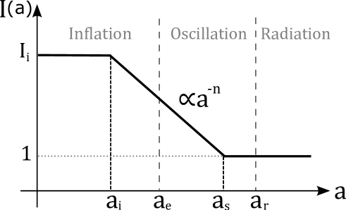
Figure 1: The behavior of $I(a)$ given in eq. (2.10). $I(a)$ decreases in proportion to $a^{-n}$ for $a_{i}<a<a_{s}$. $I$ starts decreasing during inflation $(a_{i}<a_{e})$ and stops varying before or the same time as the reheating completion $(a_{e}<a_{s}\leq a_{r})$. We mainly consider $n=3$ which produces scale-invariant magnetic fields.

To solve the above EoM, we need to specify the time evolution of $I(\chi)$. We assume that $I$ is constant at the beginning, starts varying at a certain time during inflation and stops evolving before or at the completion of reheating. We set $I=1$ when it stops such that the above field is canonically normalized at late time and normal electromagnetism is restored. The behavior of the background cosmic expansion and the kinetic function $I$ are given by

$$\eta =\left\{\begin{array}[]{lc}-1/aH_{\rm inf}\ \propto a^{-1}&(a<a_{e})\\ 2/aH\qquad\propto a^{1/2}&(a_{e}<a<a_{r})\end{array}\right.,$$ (2.6)

$$I(\eta) =\left\{\begin{array}[]{lc}(a_{i}/a_{r})^{-n}\equiv I_{i}&(a<a_{i})\\ (a(\eta)/a_{s})^{-n}&(a_{i}<a<a_{s})\\ 1&\quad(a_{s}<a)\\ \end{array}\right.,$$ (2.10)

where $a_{i},a_{e},a_{s}$ and $a_{r}$ denote the values of scale factor $a$ when $I(\eta)$ starts varying, when inflation ends, when $I$ stops evolving and when reheating completes, respectively. Fig. 1 illustrates this behavior of $I(a)$. During reheating we assume a simple matter-dominated expansion, $a\propto\eta^{2}$. It should also be stressed that our scenario is free from the strong coupling problem [19] for $n\geq 0$, because $I$ is never smaller than unity.

2.2 Solving the dynamics of the electromagnetic field

Substituting eq. (2.10) into (2.3), one finds the EoM for the gauge field mode function reads

$$\left[\partial_{\eta}^{2}+k^{2}\right](I_{i}\mathcal{A}_{\pm}^{\rm BD})= 0\,,\qquad(a<a_{i})$$ (2.11)

$$\left[\partial_{\eta}^{2}+k^{2}\pm 2\xi\frac{k}{\eta}-\frac{n(n-1)}{\eta^{2}}\right](I\mathcal{A}_{\pm}^{\rm inf})= 0\,,\qquad(a_{i}<a<a_{e})$$ (2.12)

$$\left[\partial_{\eta}^{2}+k^{2}\mp 4\xi\frac{k}{\eta}-\frac{2n(2n+1)}{\eta^{2}}\right](I\mathcal{A}_{\pm}^{\rm osc})= 0,\qquad(a_{e}<a<a_{s})$$ (2.13)

$$\left[\partial_{\eta}^{2}+k^{2}\right]\mathcal{A}_{\pm}^{\rm fin}= 0\,,\qquad(a_{s}<a)$$ (2.14)

with

$$\xi\equiv n\gamma.$$ (2.15)

We solve the EoMs with Bunch-Davies initial conditions for $a<a_{i}$,

$$I_{i}\mathcal{A}_{\pm}^{\rm BD}(a<a_{i})=\frac{e^{-ik\left(\eta-\eta_{i}\right)}}{\sqrt{2k}}\;,$$ (2.16)

where the constant phase $e^{ik\eta_{i}}$ is added for the convenience of calculation. The solutions for $a>a_{i}$ can be obtained in the usual way; after finding the general solution of the differential equation, one can fix the integration constants with the junction condition,

$$\mathcal{A}_{\pm}^{\rm before}(\eta_{*})=\mathcal{A}_{\pm}^{\rm after}(\eta_{*}),\qquad\partial_{\eta}\mathcal{A}_{\pm}^{\rm before}(\eta_{*})=\partial_{\eta}\mathcal{A}_{\pm}^{\rm after}(\eta_{*}),$$ (2.17)

where $\eta_{*}$ is one of the junction points, $\eta_{i},\eta_{e}$ or $\eta_{s}$, and $\mathcal{A}_{\pm}^{\rm before}$ and $\mathcal{A}_{\pm}^{\rm after}$ are the mode functions earlier and later than that time, respectively. We calculate the solutions during inflation and during the inflaton oscillation phase in order.

2.2.1 During inflation: $a_{i}<a<a_{e}$

The general solution for eq. (2.12) is given by

$$I\mathcal{A}_{\pm}^{\rm inf}=\frac{1}{\sqrt{2k}}\left[C_{1}^{\pm}\,M_{\mp i\xi,n-\frac{1}{2}}(2ik\eta)+C_{2}^{\pm}\,W_{\mp i\xi,n-\frac{1}{2}}(2ik\eta)\right],$$ (2.18)

where $M_{\alpha,\beta}(z)$ and $W_{\alpha,\beta}(z)$ are the Whittaker functions [44] and $C_{1}^{\pm},C_{2}^{\pm}$ are integration constants. Solving the junction condition, $\mathcal{A}_{\pm}^{\rm BD}(\eta_{i})=\mathcal{A}_{\pm}^{\rm inf}(\eta_{i})$ and $\partial_{\eta}\mathcal{A}_{\pm}^{\rm BD}(\eta_{i})=\partial_{\eta}\mathcal{A}_{\pm}^{\rm inf}(\eta_{i})$, we obtain

$$C_{1}^{\pm} =\frac{\Gamma(n\pm i\xi)}{2ik\eta_{i}\Gamma(2n)}\left[W_{1\mp i\xi,n-\frac{1}{2}}(2ik\eta_{i})+(n\mp i\xi-2ik\eta_{i})W_{\mp i\xi,n-\frac{1}{2}}(2ik\eta_{i})\right],$$ (2.19)

$$C_{2}^{\pm} =\frac{\Gamma(n\pm i\xi)}{2ik\eta_{i}\Gamma(2n)}\left[(n\mp i\xi)M_{1\mp i\xi,n-\frac{1}{2}}(2ik\eta_{i})-(n\mp i\xi-2ik\eta_{i})M_{\mp i\xi,n-\frac{1}{2}}(2ik\eta_{i})\right].$$ (2.20)

In the sub-horizon limit $|k\eta_{i}|\gg 1$, eq. (2.20) becomes $C_{2}^{\pm}\simeq e^{\pm\frac{1}{2}\pi\xi}$ which reflects the parity violation of the last term in eq. (2.1). In the super-horizon limit $|k\eta_{i}|\ll 1$, however, $C_{2}^{\pm}\simeq\Gamma(n\pm i\xi)|2k\eta_{i}|^{n}/\Gamma(2n)$ suppresses the both polarization modes.

2.2.2 During the oscillation era: $a_{e}<a<a_{s}$

The general solution for eq. (2.13) is given by

$$I\mathcal{A}_{\pm}^{\rm osc}=\frac{1}{\sqrt{2k}}\left[D_{1}^{\pm}\,M_{\pm 2i\xi,2n+\frac{1}{2}}(2ik\eta)+D_{2}^{\pm}\,W_{\pm 2i\xi,2n+\frac{1}{2}}(2ik\eta)\right],$$ (2.21)

where $D_{1}^{\pm}$ and $D_{2}^{\pm}$ are integration constants. The junction condition at the end of inflation $a=a_{e}$ is $\mathcal{A}_{\pm}^{\rm inf}(\eta_{e})=\mathcal{A}_{\pm}^{\rm osc}(\tilde{\eta}_{e}),\partial_{\eta}\mathcal{A}_{\pm}^{\rm inf}(\eta_{e})=\partial_{\eta}\mathcal{A}_{\pm}^{\rm osc}(\tilde{\eta}_{e})$. It should be noted that the conformal time $\eta$ is not continuous here. Requiring that the scale factor $a$ and Hubble parameter $H$ are continuous, one finds that the conformal time $\eta$ jumps as

$$\eta_{e}=-\frac{1}{a_{e}H_{\rm inf}}\quad{\rm(end\ of\ inflation)}\quad\Longrightarrow\quad\tilde{\eta}_{e}=\frac{2}{a_{e}H_{\rm inf}}\quad{\rm(onset\ of\ oscillation)}.$$ (2.22)

Solving the above junction condition, we obtain general expressions for $D_{1}^{\pm}$ and $D_{2}^{\pm}$ which are lengthy. However, since we are interested only in modes that exit the horizon during inflation, we need the super-horizon limits (i.e. $-k\eta_{e}\ll 1$) of $D_{1}^{\pm}$ and $D_{2}^{\pm}$,

$$D_{1}^{\pm} \simeq\frac{2^{-5n}\Gamma(2n)}{(4n+1)\Gamma(n\pm i\xi)}|k\eta_{e}|^{-3n}C_{2}^{\pm},$$ (2.23)

$$D_{2}^{\pm} \simeq 3\cdot 2^{3n+1}\frac{\Gamma(2n-1)\Gamma(2n+1\mp 2i\xi)}{\Gamma(4n+2)\Gamma(n\pm i\xi)}\left|k\eta_{e}\right|^{n+1}C_{2}^{\pm}.$$ (2.24)

Here, the both are proportional to $C_{2}$, because the second term in eq. (2.18) is the growing mode while the term proportional to $C_{1}$ can be neglected at the end of inflation. On the other hand, after inflation the first term in eq. (2.21) is the growing mode since $|k\eta|$ is now increasing.

2.2.3 After $I$ stops evolving: $a_{s}<a$

The general solution for eq. (2.14) is a free electromagnetic wave as in Minkowski spacetime,

$$\mathcal{A}_{\pm}^{\rm fin}=\frac{1}{\sqrt{2k}}\left[F_{1}^{\pm}e^{ik(\eta-\eta_{s})}+F_{2}^{\pm}e^{-ik(\eta-\eta_{s})}\right],$$ (2.25)

where $F_{1}$ and $F_{2}$ are integration constants. The junction condition when $I$ stops evolving at $a=a_{s}$ is $\mathcal{A}_{\pm}^{\rm osc}(\eta_{s})=\mathcal{A}_{\pm}^{\rm fin}(\eta_{s}),\partial_{\eta}\mathcal{A}_{\pm}^{\rm osc}(\eta_{s})=\partial_{\eta}\mathcal{A}_{\pm}^{\rm fin}(\eta_{s})$. Solving this junction condition, we obtain

$$F_{1}^{\pm} =\frac{-i}{2k\eta_{s}}\Big{[}2D_{1}^{\pm}(ik\eta_{s}+n-i\xi)M_{2i\xi,2n+\frac{1}{2}}+D_{1}^{\pm}(2n+2i\xi+1)M_{2i\xi+1,2n+\frac{1}{2}}$$

$$\qquad\qquad+2D_{2}^{\pm}(ik\eta_{s}+n-i\xi)W_{2i\xi,2n+\frac{1}{2}}-D_{2}^{\pm}W_{2i\xi+1,2n+\frac{1}{2}}\Big{]},$$ (2.26)

$$F_{2}^{\pm} =\frac{i}{2k\eta_{s}}\Big{[}2D_{1}^{\pm}(n-i\xi)M_{2i\xi,2n+\frac{1}{2}}+D_{1}^{\pm}(2n+2i\xi+1)M_{2i\xi+1,2n+\frac{1}{2}}$$

$$\qquad\qquad+2D_{2}^{\pm}(n-i\xi)W_{2i\xi,2n+\frac{1}{2}}-D_{2}^{\pm}W_{2i\xi+1,2n+\frac{1}{2}}\Big{]},$$ (2.27)

where all the suppressed arguments of the Whittaker functions are $2ik\eta_{s}$. It is interesting to note that the mode function is proportional to the sin function in the super-horizon limit,

$$\mathcal{A}_{\pm}^{\rm fin}(\eta)\simeq\frac{2^{1-n}\Gamma(2n)}{\sqrt{2k}\,\Gamma(n\pm i\xi)}|k\eta_{e}|^{-n}\left(\frac{a_{s}}{a_{e}}\right)^{n}C_{2}^{\pm}\,\sin(k(\eta-\eta_{s})),\qquad(|k\eta_{s}|\ll 1)$$ (2.28)

This is because $\mathcal{A}_{\pm}^{{\rm osc}}$ was increasing and did not have a constant part which would be inherited by the coefficient of $\cos(k(\eta-\eta_{s}))$. For $k\eta_{s}\ll k\eta\ll 1$, the mode function grows as $\mathcal{A}_{\pm}^{\rm fin}\propto\eta\propto a^{1/2}$ until it reaches the maximum value of the constant oscillation for the first time. This slows down the dilution of the magnetic energy density on super-horizon scales from $a^{-4}$ into $a^{-3}$, unless the electric conductivity affects its dynamics. This fact was recently also noticed in Ref. [45].

2.3 The electromagnetic spectra

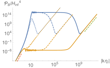
Figure 2: $\mathcal{P}_{B}(k,\eta)/H_{{\rm inf}}^{4}$ (left panel) and $\mathcal{P}_{E}(k,\eta)/H_{{\rm inf}}^{4}$ (right panel) of the $+$ (blue) and $-$ (yellow) polarization modes are plotted for $n=3$ and $\xi=7.6$ during inflation. The time evolution is shown for $a/a_{i}=10$ (dotted), $10^{4}$ (dashed) and $10^{8}$ (solid). One can see that only the + mode (blue) is amplified around the horizon crossing due to the tachyonic instability, and both magnetic modes stay constant on super-horizon scales. Hence, a scale-invariant helical magnetic field is produced. However, the modes which have already exited the horizon before $I$ starts varying, $|k\eta_{i}|\lesssim 1$, are not amplified and have a very blue spectrum $\mathcal{P}_{B}\propto k^{6}$. The red and green dashed lines show $k^{6}$ and $k^{4}$ dependence as references, respectively.

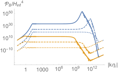
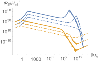
Figure 3: The same figure as Fig. 2 but during the inflaton oscillation era after inflation. We set $a_{e}/a_{i}=10^{12}$ and the spectra are shown at three different times, $a/a_{e}=1$ (dotted), $10^{3}$ (dashed) and $10^{6}$ (solid). The super-horizon modes continue to increase. Furthermore, the $+$ modes are further amplified by the tachyonic instability when they re-enter the horizon. The small wiggles are due to the oscillations of the modes on sub-horizon scales. In this figure electric conductivity which can stop the time evolution of the electromagnetic fields before $a_{s}$ is not taken into account. For our fiducial parameters, amplification is terminated by conductivity at $a/a_{e}\simeq 10^{4}$ as we will see in Sec. 4. The peak value of $\mathcal{P}_{E}$ is then much smaller than $M_{\rm Pl}^{2}H_{{\rm inf}}^{2}\approx 10^{54}H_{{\rm inf}}^{4}[(10^{5}{\rm GeV})^{4}/\rho_{\rm inf}]$ and backreaction can be safely ignored for sufficiently low inflation scales.

Having these analytic solutions of $\mathcal{A}_{\pm}(\eta)$, we can compute the power spectra of the electromagnetic fields and their time evolution. We introduce the power spectra of the electric and magnetic fields for each polarization as

$$\mathcal{P}_{E}^{\pm}(\eta,k)\equiv\frac{k^{3}I^{2}}{2\pi^{2}a^{4}}|\partial_{\eta}\mathcal{A}_{\pm}|^{2}\;,\qquad\mathcal{P}_{B}^{\pm}(\eta,k)\equiv\frac{k^{5}I^{2}}{2\pi^{2}a^{4}}|\mathcal{A}_{\pm}|^{2}\,.$$ (2.29)

Of course, the total power spectra are the sums, $\mathcal{P}_{E}=\mathcal{P}_{E}^{+}+\mathcal{P}_{E}^{-},\ \mathcal{P}_{E}=\mathcal{P}_{B}^{+}+\mathcal{P}_{B}^{-}$. Using the asymptotic behavior of the Whittaker functions, one can show that the electromagnetic power spectra in the super-horizon limit are given by

$$\mathcal{P}_{B}^{{\rm inf}}(\eta,k) \xrightarrow{|k\eta|\ll 1}\frac{H_{\rm inf}^{4}}{2^{2n}\pi^{2}}\left|\frac{\Gamma(2n-1)}{\Gamma(n+i\xi)}\right|^{2}\,|C_{2}^{\pm}|^{2}|k\eta|^{6-2n},$$ (2.30)

$$\mathcal{P}_{E}^{{\rm inf}}(\eta,k) \xrightarrow{|k\eta|\ll 1}\frac{H_{\rm inf}^{4}}{2^{2n-2}\pi^{2}}\left|\frac{\Gamma(2n)}{\Gamma(n+i\xi)}\right|^{2}\,|C_{2}^{\pm}|^{2}|k\eta|^{4-2n},$$ (2.31)

$$\mathcal{P}_{B}^{{\rm osc}}(\eta,k) \xrightarrow{|k\eta|\ll 1}\frac{2^{2-2n}H_{\rm inf}^{4}}{(4n+1)^{2}\pi^{2}}\left|\frac{\Gamma(2n)}{\Gamma(n+i\xi)}\right|^{2}\,|C_{2}^{\pm}|^{2}\left(\frac{k}{a_{e}H_{\rm inf}}\right)^{6-2n}\left(\frac{a}{a_{e}}\right)^{2n-3},$$ (2.32)

$$\mathcal{P}_{E}^{{\rm osc}}(\eta,k) \xrightarrow{|k\eta|\ll 1}\frac{H_{\rm inf}^{4}}{2^{2n}\pi^{2}}\left|\frac{\Gamma(2n)}{\Gamma(n+i\xi)}\right|^{2}\,|C_{2}^{\pm}|^{2}\left(\frac{k}{a_{e}H_{\rm inf}}\right)^{4-2n}\left(\frac{a}{a_{e}}\right)^{2n-4},$$ (2.33)

$$\mathcal{P}_{B}^{\rm fin}(\eta,k) \xrightarrow{|k\eta|\ll 1}\frac{H_{\rm inf}^{4}}{2^{2n-2}\pi^{2}}\left|\frac{\Gamma(2n)}{\Gamma(n+i\xi)}\right|^{2}\,|C_{2}^{\pm}|^{2}\left(\frac{k}{a_{e}H_{\rm inf}}\right)^{6-2n}\left(\frac{a_{s}}{a_{e}}\right)^{2n-3}\left(\frac{a}{a_{s}}\right)^{-3},$$ (2.34)

$$\mathcal{P}_{E}^{\rm fin}(\eta,k) \xrightarrow{|k\eta|\ll 1}\frac{H_{\rm inf}^{4}}{2^{2n}\pi^{2}}\left|\frac{\Gamma(2n)}{\Gamma(n+i\xi)}\right|^{2}\,|C_{2}^{\pm}|^{2}\left(\frac{k}{a_{e}H_{\rm inf}}\right)^{4-2n}\left(\frac{a_{s}}{a_{e}}\right)^{2n-4}\left(\frac{a}{a_{s}}\right)^{-4},$$ (2.35)

where $n>1/2$ is assumed and the asymptotic form of $D_{1}$ eq. (2.23) is used. The magnetic power spectrum $\mathcal{P}_{B}$ is always proportional to $k^{6-2n}$. Therefore if we set $n=3$, a scale-invariant magnetic fields will be generated for $-\eta_{i}^{-1}\ll k\ll\eta^{-1}$,

$$n=3\quad\Longrightarrow\quad{\rm Scale\ invarinant\ MF}.$$ (2.36)

In Figs. 2-3, we illustrate the time evolution of the power spectra $\mathcal{P}_{E,B}^{\pm}$ for the case $n=3$ and $\xi=7.6$ without using super/sub-horizon approximations. It is confirmed that scale-invariant magnetic fields are generated and that the above analytic expressions in the super-horizon limit are good approximations.

3 Electric Conductivity

In the previous section, we have determined the evolution of the electromagnetic field in our model. However, in these calculation they are still electromagnetic waves in which electric and magnetic fields oscillate into each other. To connect them to the present cosmic magnetic fields, we need to consider the electric conductivity which induces a conversion of electromagnetic waves into frozen magnetic fields and completely damps the electric field. In this section, we introduce conductivity and solve the dynamics of the electromagnetic fields in a highly conducting plasma as the generated during reheating.

3.1 The effect of conductivity on magnetogenesis

We consider the interaction between the charge current and the electromagnetic field in our model lagrangian eq. (2.1),

$$\mathcal{L}_{\rm int}=-J^{\mu}A_{\mu},$$ (3.1)

where the current is phenomenologically given by [43]

$$J_{\mu}=\rho_{e}u_{\mu}+\sigma_{c}E_{\mu},$$ (3.2)

where $\rho_{e}$ is the charge density which is assumed to be negligible for the neutrality of the universe on the scale in interest. Here the electric conductivity $\sigma_{c}$ is introduced as a proportionality constant between the current density and the electric field, $\bm{J}=\sigma_{c}\bm{E}$ (see Appendix. A for a derivation). In Coulomb gauge, this new term in the Lagrangian Eq. (3.1) modifies the EoM for photon, Eq. (2.3), into

$$\partial_{\eta}^{2}\mathcal{A}_{\pm}+\left[2\frac{\partial_{\eta}I}{I}+\frac{a\sigma_{c}}{I^{2}}\right]\partial_{\eta}\mathcal{A}_{\pm}+\left[k^{2}\pm 2\gamma k\frac{\partial_{\eta}I}{I}\right]\mathcal{A}_{\pm}=0,$$ (3.3)

where we have used $E_{i}=-\dot{A}_{i}=-a^{-1}\partial_{\eta}A_{i}$. Changing the time variable to cosmic time, $dt=ad\eta$, the above EoM can be written as

$$\ddot{\mathcal{A}}_{\pm}+\left[H+\frac{\sigma_{c}}{I^{2}}+2\frac{\dot{I}}{I}\right]\dot{\mathcal{A}}_{\pm}+\left[\frac{k^{2}}{a^{2}}\pm 2\gamma\frac{k}{a}\frac{\dot{I}}{I}\right]\mathcal{A}_{\pm}=0.$$ (3.4)

In this expression one sees that $\sigma_{c}>0$ works as a friction term, while $\dot{I}/I=-nH<0$ is amplifying the electromagnetic fields and can be interpreted as a “negative friction”. Note that since $\sigma_{c}$ is divided by $I^{2}$, the conductivity term is suppressed for $I\gg 1$. This is because, in the weak coupling regime ($I\gg 1$), electric conductivity which is caused by the coupling to the charged current becomes inefficient.

To understand how the electric conductivity affects the generation of the electromagnetic fields, we analyze a simple but sufficiently general case which is analytically solvable. In addition to the assumption $I=(\eta/\eta_{s})^{-2n}$ for $\eta_{e}<\eta<\eta_{s}$ and $I=1$ for $\eta_{s}<\eta$ (see eq. (2.10)), we also assume power-law time dependence for the conductivity after inflation,

$$\sigma_{c}(\eta)=\sigma_{r}\left(\frac{a}{a_{r}}\right)^{m}=\sigma_{r}\left(\frac{\eta}{\eta_{r}}\right)^{2m}\qquad(\eta_{e}<\eta\leq\eta_{r})\,,$$ (3.5)

where $m$ is a constant and $\sigma_{r}$ is the conductivity at the reheating completion. With this ansatz, the conductivity term in Eq. (3.3) becomes

$$\frac{a\sigma_{c}}{I^{2}}=\frac{2\sigma_{r}}{H_{r}\eta_{r}}\left(\frac{\eta}{\eta_{r}}\right)^{2m+2}\times\begin{cases}(\eta/\eta_{s})^{4n}&(\eta_{e}<\eta<\eta_{s})\\ 1&(\eta_{s}<\eta\leq\eta_{r})\,.\\ \end{cases}$$ (3.6)

After the end of inflation and before $I$ stops varying, $\eta_{e}<\eta<\eta_{s}$, Eq. (3.3) reads

$$\partial_{\eta}^{2}\mathcal{A}_{\pm}+\frac{4n}{\eta}\left[-1+\left(\frac{\eta}{\bar{\eta}_{c}}\right)^{2m+4n+3}\right]\partial_{\eta}\mathcal{A}_{\pm}+\left[k^{2}\mp\gamma k\frac{4n}{\eta}\right]\mathcal{A}_{\pm}=0,$$ (3.7)

where the conductivity term becomes comparable to the negative friction term at $\bar{\eta}_{c}$,

$$\bar{\eta}_{c}=\left[2n\frac{H_{r}}{\sigma_{r}}\,\eta_{r}^{2m+3}\eta_{s}^{4n}\right]^{\frac{1}{2m+4n+3}}.$$ (3.8)

Note if this expression results in $\bar{\eta}_{c}\gg\eta_{s}$, conductivity is always negligible while $I$ is varying.

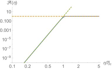
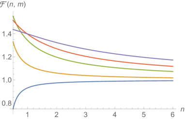
Figure 4: (Left panel) The analytic solution eq. (3.9) is shown as blue solid line for $G_{1}=1,n=3$ and $\ell=15$. The asymptotic forms, $\mathcal{A}(\eta\ll\eta_{c})=4n(\eta/\eta_{c})^{4n+1}/(\ell\Gamma(\frac{4n+\ell+1}{\ell}))$ and $\mathcal{A}(\eta\gg\eta_{c})=1$, are also plotted as dashed lines. One can see that the growth of $\mathcal{A}(\eta)$ is terminated by the electric conductivity at $\eta\simeq\bar{\eta}_{c}$. (Right panel) $\mathcal{F}(n,m)$ introduced in Eq. (3.12). The horizontal axis denotes $n$ and the colored lines represent $m=-2$ (blue), $-3/2$ (orange), $-1/4$ (green), $1$ (red) and $3$ (purple) from bottom to top. $\mathcal{F}(n,m)\simeq 1$ holds in broad parameter space.

Focusing on super-horizon modes and ignoring the third term, eq. (3.7) can be analytically solved as

$$\mathcal{A}(\eta)=G_{1}+G_{2}\,\Gamma\left(\frac{4n+1}{\ell},\,\frac{4n}{\ell}\,\left(\frac{\eta}{\bar{\eta}_{c}}\right)^{\ell}\right),\qquad(\eta_{e}<\eta<\eta_{s})$$ (3.9)

where $\ell\equiv 2m+4n+3$, $G_{1}$ and $G_{2}$ are integration constants, and $\Gamma(a,x)$ is the incomplete Gamma function. Here we drop the label of the circular polarization $\lambda=\pm$. This solution is shown in the left panel of Fig. 4. Using the asymptotic behavior of the incomplete Gamma function,

$$\Gamma(a,x)=\begin{cases}\Gamma(a)-x^{a}/a&(x\to 0)\\ x^{a-1}\exp[-x]&(x\to\infty)\\ \end{cases},$$ (3.10)

one finds that the asymptotic behavior of Eq. (3.9) is

$$\mathcal{A}(\eta)=\begin{cases}G_{1}+G_{2}\Gamma(\frac{4n+1}{\ell})-G_{2}\frac{\ell}{4n+1}\left(\frac{4n}{\ell}\right)^{\frac{4n+1}{\ell}}\,\left(\frac{\eta}{\bar{\eta}_{c}}\right)^{4n+1}&(\eta\ll\bar{\eta}_{c})\\ G_{1}+G_{2}\,\left(\frac{4n}{\ell}\right)^{\frac{4n+1}{\ell}-1}\left(\frac{\eta}{\bar{\eta}_{c}}\right)^{4n+1-\ell}\exp\left[-\frac{4n}{\ell}\,\left(\frac{\eta}{\bar{\eta}_{c}}\right)^{\ell}\right]&(\eta\gg\bar{\eta}_{c})\\ \end{cases}.$$ (3.11)

The integration constants $G_{1}$ and $G_{2}$ are constrained to $G_{1}+G_{2}\Gamma(\frac{4n+1}{\ell})=0$ by requiring the mode function to reproduce the behavior without conductivity (i.e. $\mathcal{A}\sim\eta^{4n+1}$ which was studied in Sec. 2.2.2) at early times, $\eta\ll\bar{\eta}_{c}$ where conductivity is negligible. On the other hand, the mode function quickly tends to a constant $G_{1}$ once conductivity becomes effective, for $\eta\gg\bar{\eta}_{c}$. Therefore, parameterizing the coefficient of the early-time behavior $\mathcal{A}\propto(\eta/\bar{\eta}_{c})^{4n+1}$ as $\mathcal{A}_{c}$, the late-time amplitude is simply $\mathcal{A}_{c}$ with an $\mathcal{O}(1)$ correction,

$$\mathcal{A}(\eta\ll\bar{\eta}_{c}<\eta_{s})\simeq\mathcal{A}_{c}\left(\frac{\eta}{\bar{\eta}_{c}}\right)^{4n+1}\quad\Longrightarrow\quad\mathcal{A}(\bar{\eta}_{c}\ll\eta<\eta_{s})=\mathcal{F}(n,m)\,\mathcal{A}_{c},$$ (3.12)

where the correction factor $\mathcal{F}(n,m)\equiv\left(\frac{\ell}{4n}\right)^{\frac{4n+1}{\ell}}\Gamma\left(1+\frac{4n+1}{\ell}\right)$ is always around unity as shown in Fig. 4. The frozen amplitude of $\mathcal{A}$ takes almost the same value as the case where the behavior without the conductivity $\mathcal{A}\propto\eta^{4n+1}$ continues up to $\eta=\bar{\eta}_{c}$ and $\mathcal{A}$ suddenly stops there. The condition that the conductivity becomes significant before $I$ stops varying is

$$\bar{\eta}_{c}<\eta_{s}\quad\Longrightarrow\quad\frac{\sigma_{r}}{H_{r}}>2n\left(\frac{\eta_{r}}{\eta_{s}}\right)^{2m+3}.$$ (3.13)

Note that the analysis so far from eq. (3.7) have considered the dynamics after the inflation end and before $I$ stops running, $\eta_{e}<\eta<\eta_{s}$. However, even later, when $I\equiv 1$, a very similar argument holds. By taking the limit $n\to 0$ in eq. (3.7), we obtain an analytic solution after $I$ stops evolving,

$$\mathcal{A}(\eta)=G_{1}+G_{2}\,\Gamma\left(\frac{1}{2m+3},\,\frac{2}{2m+3}\,\left(\frac{\eta}{\tilde{\eta}_{c}}\right)^{2m+3}\right),\qquad(\eta_{s}<\eta<\eta_{r}).$$ (3.14)

with

$$\tilde{\eta}_{c}=\left(H_{r}/\sigma_{r}\right)^{\frac{1}{(2m+3)}}\eta_{r}.$$ (3.15)

As early time limit $\eta/\tilde{\eta}_{r}\to 0$, eq. (3.14) has a constant mode and a growing mode which is proportional to $\eta$. As discussed below eq. (2.28), the super-horizon mode obeys $\mathcal{A}^{\rm fin}\propto\eta$ in this regime without the conductivity. Hence, the same argument as eq. (3.12) yields in this case

$$\mathcal{A}(\eta_{s}<\eta\ll\tilde{\eta}_{c})\simeq\tilde{\mathcal{A}}_{c}\frac{\eta}{\tilde{\eta}_{c}}\quad\Longrightarrow\quad\mathcal{A}(\eta_{s}<\tilde{\eta}_{c}\ll\eta)=\tilde{\mathcal{F}}(m)\,\tilde{\mathcal{A}}_{c},$$ (3.16)

where the correction factor now is $\tilde{\mathcal{F}}(m)=2^{\frac{-1}{2m+3}}(2m+3)^{-\frac{2m+2}{2m+3}}\Gamma(\frac{1}{2m+3})$ which is always close to unity for $m\gtrsim-1$. Therefore, in a similar way to the case with $\bar{\eta}_{c}<\eta_{s}$, the electric conductivity freezes the magnetic fields on super horizon scales when it becomes significant at $\eta=\tilde{\eta}_{c}>\eta_{s}$.

3.2 When does conductivity terminate magnetogenesis?

In the previous subsection, we solved the dynamics of the electromagnetic field under the effect of the electric conductivity and found that it terminates the growth of the mode function $\mathcal{A}_{\pm}$. To calculate the final amplitude of the magnetic fields, therefore, it is crucial to estimate when the conductivity becomes significant. We have given expressions for this time in terms of, $\bar{\eta}_{c}$ and $\tilde{\eta}_{c}$ in eqs. (3.8) and (3.15), depending on whether conductivity becomes efficient during magnetogenesis or only after, we now define $\eta_{c}$ as the unified variable

$$\eta_{c}\equiv\begin{cases}\left[2n\frac{H_{r}}{\sigma_{r}}\,\left(\frac{\eta_{r}}{\eta_{s}}\right)^{2m+3}\right]^{1/\ell}\eta_{s}&\qquad\left(\sigma_{r}/H_{r}\gg\left(\eta_{r}/\eta_{s}\right)^{2m+3}\right)\\ \left(\frac{H_{r}}{\sigma_{r}}\right)^{\frac{1}{(2m+3)}}\eta_{r}&\qquad\left(\sigma_{r}/H_{r}\lesssim\left(\eta_{r}/\eta_{s}\right)^{2m+3}\right)\,.\\ \end{cases}$$ (3.17)

In this equation, two dimensionless parameters, $\sigma_{r}/H_{r}$ and $m$ are involved. To develop our understanding of $\eta_{c}$, we now determine these parameters.

We first compute $\sigma_{r}/H_{r}$. It has been known that the conductivity from charged particles in thermal equilibrium is given by [46]

$$\sigma_{c}=c_{\sigma}T,\qquad c_{\sigma}\simeq\alpha_{e}^{-1}\approx 10^{2},$$ (3.18)

where $\alpha_{e}$ is the fine structure constant. Once reheating is completed, $\eta=\eta_{r}$, the universe is dominated by radiation and its energy density is $\rho_{\rm rad}=3M_{\rm Pl}^{2}H_{r}^{2}=\pi^{2}g_{*}T_{r}^{4}/30$, where $T_{r}$ is the reheating temperature. Hence, we find that the conductivity at $\eta_{r}$ is given by

$$\frac{\sigma_{r}}{H_{r}}=c_{\sigma}\left(\frac{90M_{\rm Pl}^{2}}{\pi^{2}g_{*}H_{r}^{2}}\right)^{\frac{1}{4}}\approx 10^{20}\,\left(\frac{T_{r}}{1{\rm GeV}}\right)^{-1}\left(\frac{c_{\sigma}}{10^{2}}\right)\left(\frac{g_{*}}{10^{2}}\right)^{-\frac{1}{2}}.$$ (3.19)

The electric conductivity largely dominates the Hubble scale at the end of reheating. Note that $\sigma_{r}/H_{r}\gg 1$ guarantees that the conductivity becomes significant before the end of reheating for $m>-3/2$ (see eq. (3.15)). Incidentally, since $T\propto a^{-1}$ and $H\propto a^{-2}$ in the radiation dominant era, the ratio $\sigma_{c}/H$ even increases after reheating.

Let us specify $m$ which parameterizes the time-dependence of $\sigma_{c}$ as given in Eq. (3.5). To calculate the temperature during reheating, we need to model how charged particles are produced. As an simple model, we consider that the inflaton decays into charged particles with constant decay rate $\Gamma_{\phi}$. The energy density of the charged particles $\rho_{\rm cp}$ for $\eta_{e}\ll\eta\ll\eta_{r}$ is then given by [47]

$$\rho_{\rm cp}\simeq\frac{6}{5}M_{\rm Pl}^{2}\Gamma_{\phi}H\propto a^{-3/2}\quad\Longrightarrow\quad\sigma_{c}\propto T\propto a^{-3/8}\quad\Longrightarrow\quad m=-\frac{3}{8},$$ (3.20)

where we used $\rho_{\rm cp}\propto T^{4}$. Note that we assumed that the decay products have reached thermal equilibrium, otherwise their temperature $T$ is ill-defined. We also discuss the out-of-equilibrium case in Appendix. A.

Let us now come back to eq. (3.17) for the present case. Setting $m=-3/8$, the boundary of the condition between the two cases of eq. (3.17) is

$$\frac{\sigma_{r}}{H_{r}}\simeq\left(\frac{\eta_{r}}{\eta_{s}}\right)^{2m+3}\quad\Longrightarrow\quad\frac{a_{r}}{a_{s}}\simeq 5\times 10^{17}\left(\frac{T_{r}}{1{\rm GeV}}\right)^{-\frac{8}{9}}\left(\frac{c_{\sigma}}{10^{2}}\right)^{\frac{8}{9}}\left(\frac{g_{*}}{10^{2}}\right)^{-\frac{4}{9}}.$$ (3.21)

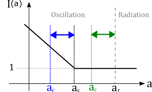
Figure 5: The two possibilities of the timing when the conductivity becomes important $a_{c}$ derived in eq. (3.22). The first and second line of eq. (3.22) corresponds to the blue and green case, respectively.

Changing $\eta_{c}$ into the scale factor, $a_{c}=a(\eta_{c})$, one can rewrite eq. (3.17) as

$$a_{c}\equiv\begin{cases}2\times 10^{-3}T_{\rm 1GeV}^{\frac{8}{57}}\,(a_{r}/a_{s})^{\frac{3}{19}}\,a_{s}&\quad\left(a_{r}/a_{s}\ll 10^{18}T_{\rm 1GeV}^{-\frac{8}{9}}\right)\\ 2\times 10^{-18}T_{\rm 1GeV}^{\frac{8}{9}}\,a_{r}&\quad\left(a_{r}/a_{s}\gtrsim 10^{18}T_{\rm 1GeV}^{-\frac{8}{9}}\right)\\ \end{cases},$$ (3.22)

where $T_{\rm 1GeV}\equiv T_{r}/(1{\rm GeV})$ and the dependences on $c_{\sigma}$ and $g_{*}$ are suppressed. This result is illustrated in fig. 5. The above equation implies that the electric conductivity terminates the growth of the magnetic fields slightly before the kinetic function $I$ stops, $1>a_{c}/a_{s}>0.002T_{\rm 1GeV}^{8/57}$, unless we have a sufficiently long time interval between the end of magnetogenesis and the end of reheating. This is due to the large kinetic function $I\gg 1$ which substantially suppresses conductivity until $I$ becomes $\mathcal{O}(1)$ at $\eta\simeq\eta_{s}$. If the time interval between $a_{s}$ and $a_{r}$ is long enough, on the other hand, the time interval between the termination of magnetogenesis and the end of reheating is given by $a_{r}/a_{c}\simeq 5\times 10^{17}T_{\rm 1GeV}^{-8/9}$, irrespective of $a_{s}$. This is simply because $a_{r}/a_{c}$ is determined by the time evolution of $\sigma_{c}$ during reheating which is fully determined by $\sigma_{c}/H_{c}$ and $m$ in this case.

4 Magnetic Fields Today

In this section, we calculate the present strength of the magnetic fields produced in our model.

4.1 Late-time evolution

Even though our magnetic fields are fully helical, an inverse cascade is not effective in the case of a (nearly) scale invariant spectrum. This has been shown by numerical simulations in [48, 49] and it is not very surprising. The inverse cascade is actually a consequence of helicity conservation. When small scale magnetic fields are damped by viscosity and Alvfén wave damping, their helicity has to move to larger scales. If the power is anyway dominated by large scale fields this is a very small effect and will not change the magnetic field spectrum on large scales significantly. Here we simply neglect this small effect.

Therefore, the magnetic power spectrum decays as $\mathcal{P}_{B}\propto a^{-4}$ after the mode function is frozen out, $\mathcal{A}_{\pm}=$const. due to electric conductivity at $\eta=\eta_{c}$. Setting $n=3$ and multiplying $\mathcal{P}_{B}(k,\eta_{c})$ by $a_{c}^{4}$, we obtain the present strength of the scale-invariant part of the produced magnetic fields as

$$\mathcal{P}_{B}^{\rm now}(k_{i}<k<k_{T},n=3)\simeq\frac{H_{\rm inf}^{4}}{2^{4}\pi^{2}}\frac{e^{\pi\xi}\,\Gamma^{2}(6)}{|\Gamma(3+i\xi)|^{2}}\,\frac{1}{a_{e}^{3}}\times\begin{cases}a_{c}^{7}&(a_{c}<a_{s})\\ a_{s}^{6}a_{c}&(a_{s}<a_{c})\\ \end{cases},$$ (4.1)

where $\mathcal{P}^{\rm osc}_{B}(k,\eta_{c})$ in eq.(2.32) or $\mathcal{P}^{\rm fin}_{B}(k,\eta_{c})$ in eq.(2.34) are used depending on whether $\eta_{c}\gtrless\ \eta_{s}$ and we approximate the correction factors $\mathcal{F}(m,n)$ and $\tilde{\mathcal{F}}(m)$ by unity. Here $k_{i}$ and $k_{T}$ denote the IR cut-off scale $k_{i}=-1/\eta_{i}$ and the turbulence scale today, respectively. Inserting numbers, one can rewrite the above equation as

$$\mathcal{P}_{B}^{\rm now}\approx 3\times 10^{-28}{\rm G}^{2}\ \frac{e^{\pi\xi}\sinh(\pi\xi)}{4\xi+5\xi^{3}+\xi^{5}}\left(\frac{\rho_{\rm inf}^{1/4}}{10^{5}{\rm GeV}}\right)^{12}\left(\frac{T_{r}}{1{\rm GeV}}\right)^{-8}\left(\frac{g_{\ast}}{10^{2}}\right)^{-\frac{7}{3}}\times\begin{cases}(a_{c}/a_{r})^{7}&(a_{c}<a_{s})\\ a_{s}^{6}a_{c}/a_{r}^{7}&(a_{s}<a_{c})\\ \end{cases},$$ (4.2)

where we evaluated $a_{e}$ and $a_{r}$ as

$$\ln\left(\frac{a_{r}}{a_{e}}\right) \approx 22.8+\frac{4}{3}\ln\left(\frac{\rho_{\rm inf}^{1/4}}{10^{5}{\rm GeV}}\right)-\frac{4}{3}\ln\left(\frac{T_{r}}{1{\rm GeV}}\right)-\frac{1}{3}\ln\left(\frac{g_{*}}{100}\right),$$ (4.3)

$$a_{r} \approx 8\times 10^{-14}\left(\frac{T_{r}}{1{\rm GeV}}\right)^{-1}\left(\frac{g_{\ast}}{100}\right)^{-1/3}.$$ (4.4)

Here, the unit conversion, $1{\rm GeV}=3.8\times 10^{9}{\rm G}^{1/2}$, is used.

4.2 Consistency conditions

For successful primordial magnetogenesis, one must satisfy the following three conditions: The scenario is free from (i) a strong coupling regime for which calculations cannot be trusted, (ii) significant back reaction from the electromagnetic fields which alters the background evolution of the universe (iii) inconsistency with CMB observations which particularly fixes the power spectrum of curvature perturbations as $\mathcal{P}_{\zeta}(k_{\rm CMB})\approx 2.2\times 10^{-9}$ with $k_{\rm CMB}=0.05{\rm Mpc}^{-1}$. Since the condition (i) is trivially satisfied in our case where $I\geq 1$, we address the backreaction problem (ii) and the curvature perturbation condition (iii).

To satisfy the backreaction condition, the energy fraction of the produced electromagnetic fields should always be a very small fraction of the energy density of the Universe,

$$\Omega_{{\rm em}}\equiv\frac{\rho_{{\rm em}}}{\rho_{{\rm tot}}}\ll 1,\qquad\rho_{\rm em}=\frac{1}{2}\int\frac{\mathrm{d}k}{k}\Big{(}\mathcal{P}_{E}(k)+\mathcal{P}_{B}(k)\Big{)},$$ (4.5)

where $\rho_{\rm tot}=3M_{\rm Pl}^{2}H^{2}$ denotes the total energy of the universe. $\Omega_{{\rm em}}(\eta)$ during the inflaton oscillation phase is written as

$$\Omega_{{\rm em}}(\eta_{e}<\eta<\eta_{r})\simeq\frac{1}{2\rho_{\rm tot}}\int\frac{\mathrm{d}k}{k}\mathcal{P}_{E}^{+}(k_{i},\eta)=e^{2N_{i}}\frac{150H_{{\rm inf}}^{2}a^{5}}{\pi^{3}M_{\rm Pl}^{2}a_{e}^{5}}\frac{\mathcal{I(\xi)}\sinh(\pi\xi)}{4\xi+5\xi^{3}+\xi^{5}},$$ (4.6)

where $N_{i}\equiv\ln(\eta_{i}/\eta_{e})$, we ignore the sub-leading contributions from $\mathcal{P}_{E}^{-}$ and $\mathcal{P}_{B}^{\pm}$ and use eq. (2.33) with $n=3$. A numerical evaluation of $\mathcal{I}(\xi)$ which contains the $k$-integral shows that it is well approximated by (see Appendix B for detail)

$$\mathcal{I}(\xi)\equiv\int_{0}^{\infty}\frac{\mathrm{d}y}{y^{3}}\,\left|C^{+}_{2}(y)\right|^{2}=\frac{e^{\pi\xi}}{\alpha\xi^{2}+\beta\xi+\gamma},\qquad\alpha\approx 4.7,\ \beta\approx 2.7,\ \gamma\approx 10,$$ (4.7)

where the dummy variable $y\equiv-k\eta_{i}$ is introduced and the numerical fit is performed for $1\leq\xi\leq 50$. $\Omega_{\rm em}$ reaches its maximum value at either $\eta_{c}$ or $\eta_{s}$ whichever is earlier. We obtain its maximum value given by

$$\Omega_{\rm em}^{\max} \simeq 10^{-2}\frac{\mathcal{I(\xi)}\sinh(\pi\xi)}{4\xi+5\xi^{3}+\xi^{5}}\left(\frac{\rho_{\rm inf}^{1/4}}{10^{5}{\rm GeV}}\right)^{12}\left(\frac{T_{r}}{1{\rm GeV}}\right)^{-6}\left(\frac{g_{\ast}}{10^{2}}\right)^{-\frac{5}{3}}\left(\frac{k_{i}}{1{\rm Mpc}^{-1}}\right)^{-2}$$ (4.8)

$$\times\begin{cases}(a_{c}/a_{r})^{5}&(a_{c}<a_{s})\\ (a_{s}/a_{r})^{5}&(a_{s}<a_{c})\,,\\ \end{cases}$$

where we used $N_{i}\approx 28+\frac{2}{3}\ln(\rho_{{\rm inf}}^{1/4}/10^{5}{\rm GeV})+\frac{1}{3}\ln(T_{r}/1{\rm GeV})-\ln(k_{i}/1{\rm Mpc}^{-1})$. A lower inflationary energy scale and higher reheating temperature decrease $\Omega_{\rm em}^{\max}$, because they shorten the inflaton oscillation phase in which $\Omega_{\rm em}\propto a^{5}$ grows rapidly. $\Omega_{\rm em}^{\max}$ also depends on the IR cut-off as $\Omega_{\rm em}^{\max}\propto k_{i}^{-2}$, because the electric power spectrum is red-tilted $\mathcal{P}_{E}\propto k^{-2}$ for $n=3$ and the dominant contribution to $\Omega_{\rm em}$ comes from the largest amplified scale $k\simeq k_{i}$. Thus, pushing the IR cut-off to smaller scales alleviates the backreaction constraint.

Dividing eq. (4.2) by the above expression, we rewrite the magnetic power spectrum today as,

$$\mathcal{P}_{B}^{\rm now} \approx 3\times 10^{-26}{\rm G}^{2}\,\Omega_{\rm em}^{\max}(\alpha\xi^{2}+\beta\xi+\gamma)\left(\frac{k_{i}}{1{\rm Mpc}^{-1}}\right)^{2}\left(\frac{T_{r}}{1{\rm GeV}}\right)^{-2}\left(\frac{g_{\ast}}{10^{2}}\right)^{-\frac{2}{3}}$$ (4.9)

$$\times\begin{cases}(a_{c}/a_{r})^{2}&(a_{c}<a_{s})\\ a_{c}a_{s}/a_{r}^{2}&(a_{s}<a_{c})\,.\\ \end{cases}$$

Before obtaining the final result for $\mathcal{P}_{B}^{\rm now}$ inserting concrete values of $\xi$ and the conductivity factor, we discuss the third consistency condition from curvature perturbations.

In the flat slicing, the curvature perturbation $\zeta$ is proportional to the energy density perturbation $\delta\rho$. The electromagnetic fields in our model contributes to its three components, $\delta\rho_{\rm em}$, $\delta\rho_{\chi}$ and $\delta\rho_{\phi}$ in different ways. First, $\delta\rho_{\rm em}$ is nothing but the energy density of the electromagnetic fields themselves. Second, since the spectator scalar field $\chi$ is directly coupled to the electromagnetic fields, its perturbation $\delta\chi$ and hence its density perturbation $\delta\rho_{\chi}\propto\delta\chi$ are induced. Third, although the inflaton $\phi$ has no direct coupling to $\chi$ or $A_{\mu}$, they are always coupled gravitationally and thus $\delta\phi$ and $\delta\rho_{\phi}\propto\delta\phi$ are affected as well. In Ref. [30], all these contributions were computed in a setup similar to ours which has the same action eq. (2.1) except for the last term. There it has been shown that the constraint from the curvature power spectrum is not stronger than the backreaction condition $\Omega_{\rm em}<10^{-1}$, if the IR cut-off is on sufficiently small scale, $k_{i}\gtrsim 1{\rm Mpc}^{-1}$ [30]. Since the dominant contribution to the curvature perturbation on the CMB scale from the electromagnetic fields is generated on super-horizon scales at which the $\phi F\tilde{F}$ term does not play an important role, we can apply the same argument as Ref. [30] to our case. Therefore, we focus on the backreaction condition henceforth.

4.3 The present magnetic field strength

$\mathcal{P}_{B}^{\rm now}$ in eq. (4.9) still depends on $a_{s}/a_{r}$, $a_{c}/a_{r}$ and $\xi$. We discuss the dependence of the scale factors based on the results of Sec. 3.2 in which $\sigma_{c}\propto a^{-3/8}$ was studied.

Considering the strong dependence of $\Omega_{\rm em}^{\max}$ on $\rho_{{\rm inf}}$, namely $\Omega_{\rm em}^{\max}\propto\rho_{{\rm inf}}^{3}$, one cannot strongly increase $\rho_{\rm inf}^{1/4}$ from $10^{5}{\rm GeV}$ in order to satisfy the backreaction consistency condition. Since the background energy density $\rho$ decreases as $a^{-3}$ during the inflaton oscillation phase, the scale factor increases during this period by a factor of $a_{r}/a_{e}\simeq 10^{7}\,T_{1{\rm GeV}}^{-4/3}\,(\rho_{{\rm inf}}^{1/4}/10^{5}{\rm GeV})^{4/3}$. This factor is much smaller than the value given in eq. (3.21) needed for conductivity not to becomes significant before the end of magnetogenesis, $\eta_{s}$. From eq. (3.22), we see that conductivity becomes significant before the stop of the kinetic function $I$ for the present parameter choice and we always have the following hierarchy of the scale factors, $a_{c}<a_{s}<a_{r}$. Then it is optimal for magnetogenesis to assume that $I$ terminates at the almost same time as reheating,

$$\frac{a_{s}}{a_{r}}\simeq 1\quad\Longrightarrow\quad\frac{a_{c}}{a_{s}}=2\times 10^{-3}T_{\rm 1GeV}^{\frac{8}{57}},$$ (4.10)

where we used the first line of eq. (3.22). Inserting the above scale factors in eq. (4.9), we obtain

$$\mathcal{P}_{B}^{\rm now} \approx 10^{-31}{\rm G}^{2}\,\Omega_{\rm em}^{\max}(\alpha\xi^{2}+\beta\xi+\gamma)\left(\frac{k_{i}}{1{\rm Mpc}^{-1}}\right)^{2}\left(\frac{T_{r}}{1{\rm GeV}}\right)^{-\frac{98}{57}},$$ (4.11)

$$\Omega_{\rm em}^{\max} \approx 3\times 10^{-16}\frac{\mathcal{I(\xi)}\sinh(\pi\xi)}{4\xi+5\xi^{3}+\xi^{5}}\left(\frac{\rho_{\rm inf}^{1/4}}{10^{5}{\rm GeV}}\right)^{12}\left(\frac{k_{i}}{1{\rm Mpc}^{-1}}\right)^{-2}\left(\frac{T_{r}}{1{\rm GeV}}\right)^{-6}.$$ (4.12)

where we suppress the dependences on $c_{\sigma}$ and $g_{*}$.

Eq. (4.11) has a positive power-law factor of $\xi$, namely $\alpha\xi^{2}+\beta\xi+\gamma$, because $\Omega_{\rm em}$ has a slightly weaker dependence on $\xi$ than $\mathcal{P}_{B}^{\rm now}$ (see the discussion in Appendix B for its reason). Consequently, a larger $\xi$ can boost the magnetic field strength $\mathcal{P}_{B}^{\rm now}$ for a given $\Omega_{\rm em}^{\max}$. However, one cannot take arbitrarily large $\xi$ due to the backreaction constraint $\Omega_{\rm em}^{\max}\ll 1$. With the fiducial parameters in eq. (4.12), $\Omega_{\rm em}^{\max}=10^{-2}$ corresponds to $\xi=7.6$ which gives $\alpha\xi^{2}+\beta\xi+\gamma\approx 3\times 10^{2}$. In that case, we obtain the present strength of the scale-invariant magnetic fields as

$$B_{\rm now}\equiv\sqrt{\mathcal{P}_{B}}\approx 6\times 10^{-16}{\rm G},$$ (4.13)

which satisfies the lower bound from blazar observations [7]. The parameters that we adopted for the result (4.13) are

$$n=3,\ \ m=-\frac{3}{8},\ \ \xi=7.6,\ \ \rho_{{\rm inf}}^{1/4}=10^{5}{\rm GeV},\ \ T_{r}=1{\rm GeV},\ \ k_{i}=1{\rm Mpc}^{-1},$$ (4.14)

as well as $c_{\sigma}=g_{*}=100.$ Note that $\mathcal{P}_{B}^{\rm now}(k)$ is scale invariant only for $k_{i}<k<k_{T}$. On larger scale $\mathcal{P}_{B}(k\ll k_{i})\propto k^{6}$ and it decays due to turbulent damping for $k\geq k_{T}$. The damping scale $\lambda_{T}\equiv 2\pi/k_{T}$ at present can be roughly estimated as [15, 50, 51]

$$\lambda_{T}\sim\frac{t_{\rm rec}B_{\rm now}}{a_{\rm rec}^{3}\sqrt{\rho_{\rm rec}}}\sim 10^{-1}{\rm pc}\left(\frac{B_{\rm now}}{10^{-15}{\rm G}}\right),$$ (4.15)

where the subscript “rec” denotes recombination. Therefore, with the above fiducial parameters, a scale-invariant magnetic field is realized on scales from $10^{-7}{\rm Mpc}$ to $1{\rm Mpc}$.

5 Summary and Discussion

In this paper we have shown that by coupling of the electromagnetic field to a spectator field during inflation, we can generate a scale invariant helical magnetic field which is sufficient not only to seed galactic and cluster fields but also satisfy the lower limit on magnetic fields in voids derived from observations of blazars [7]. To achieve this it is important that the spectator fields keeps rolling during reheating, nearly until the end. Furthermore, the production of charged particles during reheating leads to the generation of conductivity, which is soon high enough to terminate further magnetogenesis. As long as $I(\chi)$ is large and we normalize it to $1$ at the end of magnetogenesis, the coupling of charged particles is very weak and so are the effects of conductivity. Nevertheless, for the parameter values studied here, it always is the relevant phenomenon to terminate magnetogenesis before $\eta_{s}$.

In this paper, we did not investigate several other phenomena related to primordial magnetogenesis which might potentially be important. Here we briefly discuss the Schwinger effect, chiral anomaly, and baryogenesis.

The Schwinger effect is the fact that a electric field which is stronger than a certain critical value (e.g. $E_{c}=m_{e}^{2}/e$ in Minkowski spacetime) decays into pairs of charged particle and anti-particle due to non-perturbative effects of QED [52]. Recently, the Schwinger effect in the expanding universe and its influence on magnetogenesis have been intensively studied [53, 54, 55, 56, 57, 58]. Since strong electric fields are produced during the inflaton oscillation era in our scenario, the Schwinger effect might be relevant. On the other hand, as discussed in Sec. 3, the electric fields are damped efficiently by the high electric conductivity when the kinetic coupling $I$ is still much larger than unity, $I(\eta_{c})\simeq 10^{8}$, in the case of our fiducial parameters. The large value of $I$ effectively suppresses the electromagnetic interaction and hence the critical value of the electric field becomes much higher. Indeed, it was shown in Ref. [57] that the Schwinger effect is negligible until $I$ is close to unity, however, the authors studied the case where magnetogenesis was driven by the inflaton. In principle, the electric conductivity can be increased by the charged particle production by the Schwinger effect and it would be interesting to explore this possibilities based on our present work.

Recently, it was pointed out that the chiral anomaly, $\partial_{\mu}J_{5}^{\mu}+(e/4\pi)^{2}F_{\mu\nu}\tilde{F}^{\mu\nu}=0$ with $J_{5}^{\mu}=\bar{\psi}\gamma^{\mu}\gamma^{5}\psi$ being the axial current of a massless charged fermion $\psi$, plays an important role in inflationary models with the $U(1)$ Chern-Simons term $\varphi F_{\mu\nu}\tilde{F}^{\mu\nu}$ [59]. The authors of Ref. [59] have explicitly shown that when helical electromagnetic fields are generated by the Chern-Simons term during inflation, the chiral asymmetry of charged fermions should also be produced such that the above chiral anomaly equation holds. The produced chiral fermions could have a significant impact on the subsequent time evolution of the magnetic fields through the chiral magnetic effect [60, 61, 62, 63, 64]. Nevertheless, if the fermions have non-negligible mass, the chiral anomaly equation is modified and the production of the chiral asymmetry can be suppressed. In particular, for a fermion mass much larger than the Hubble scale during inflation $H_{{\rm inf}}\simeq 2{\rm eV}\,(\rho_{{\rm inf}}^{1/4}/10^{5}{\rm GeV})^{2}$, the fermion production is highly suppressed [65]. In addition, since the large $I$ effectively reduces the electromagnetic coupling $e$ into $e/I$, the fermion production may be further suppressed. Therefore, we expect that the production of the chiral asymmetry can be ignored in the parameter region relevant for our scenario.

Even if the chiral asymmetry is not generated during inflation, helical magnetic fields can cause another fascinating phenomenon around the electroweak phase transition through the chiral anomaly: The observed baryon asymmetry of our universe can be generated by (hyper-)magnetic fields, if the helicity is negative and the strength is appropriate [66, 67, 68, 69, 70, 71]. Unfortunately, however, we cannot easily apply the results of previous works to our model, mainly because the kinetic coupling $I$ has not yet become unity at the electroweak phase transition $T\simeq 10^{2}{\rm GeV}$ in our case. Another difference to existing works is that the helical magnetic field does not undergo the inverse cascade process due to its large correlation length. Thus a dedicated investigation is needed to determine the baryon asymmetry produced in our case. We leave it for a future project.

Appendix A Derivation of the Electric Conductivity

Here, we derive the electric conductivity $\sigma_{c}$ by extending the argument in Ref. [72]. The EoM for a charged particle with Lorentz force is

$$m_{e}\frac{\mathrm{d}u^{\mu}}{\mathrm{d}\tau}=eF^{\mu\nu}u_{\nu},$$ (A.1)

where $m_{e},e$ and $u^{\mu}=\gamma(1,\bm{v})$ are mass, 4-velocity and charge of the particle, and $\gamma\equiv 1/\sqrt{1-v^{2}}$ is the Lorentz factor. Averaging this equation over a fluid element which contains many charged particles with random velocity directions, one finds that the terms proportional to the velocity vector becomes negligible. However, since the acceleration due to the homogeneous electric field remains, we obtain

$$\frac{\mathrm{d}\bar{\bm{v}}}{\mathrm{d}t}=\frac{e}{p}\bm{E},$$ (A.2)

where $p=\gamma m_{e}$ is the typical momentum of the particles and $\bar{\bm{v}}$ denotes the averaged velocity. Provided that the particles are monotonically accelerated by the electric field for a time $t_{a}$, the averaged velocity is the order of $\bar{\bm{v}}\simeq t_{a}e\bm{E}/p$. Therefore, the averaged current density $\bm{J}$ is expressed in terms of the electric field as

$$\bm{J}\simeq en\bar{\bm{v}}\simeq t_{a}\frac{e^{2}n}{p}\bm{E}\quad\Longrightarrow\quad\sigma_{c}=t_{a}\frac{e^{2}n}{p},$$ (A.3)

where $n$ is the number density of the charged particles.

The acceleration time $t_{a}$ is often evaluated as the collision time (or the mean free path) which is the inverse of the interaction rate of the charged particles $\Gamma_{c}$. However, if the interaction of the charged particles is not significant within the Hubble time, it is more reasonable to estimate $t_{a}$ as an order of the Hubble time, because the acceleration time cannot be longer than the lifetime of the universe. Thus we have

$$t_{a}\simeq(\max[\Gamma_{c},H])^{-1}.$$ (A.4)

It should be noted that if the interaction rate $\Gamma_{c}$ is larger than $H$, the particles are expected to be in thermal equilibrium. In this case $\Gamma_{c}>H$, using $p\simeq T$ and $t_{a}\simeq T^{2}/(e^{4}n)$, one finds [72]

$$\sigma_{\rm thermal}\simeq\frac{T}{e^{2}},\qquad({\rm thermal\ equilibrium})$$ (A.5)

where $T$ is the temperature of the thermal bath. This expression agrees with eq. (3.18) aside from the constant numerical factor. In the other case $H>\Gamma_{c}$, the conductivity is given by

$$\sigma_{\rm non-thermal}\simeq\frac{e^{2}n}{Hp}.\qquad({\rm out\ of\ thermal\ equilibrium})$$ (A.6)

Since we have already discussed the thermalized case in Sec. 3.2, here we consider the case where the electric conductivity is induced by charged particles out of equilibrium. Again, to compute a concrete time dependence of $\sigma_{c}$ from eq. (A.6), a model of the particle production is necessary. For simplicity, we make the same assumption as eq. (3.20) that inflaton decays into the charged particles with a constant decay rate $\Gamma_{\phi}$. Note that the difference from the previous case is that the interaction between the decay products are not strong enough to reach thermal equilibrium. If the inflaton mass is much larger than the charged particle mass, $m_{\phi}\gg m_{e}$, the momentum of the produced particle is the order of the inflaton mass $p\simeq m_{\phi}$. Then, the particle number density is $n\simeq\rho_{\rm rad}/p\simeq M_{\rm Pl}^{2}\Gamma_{\phi}H/m_{\phi}$. Finally using $m_{\phi}\simeq H_{{\rm inf}}$ and $\Gamma_{\phi}\simeq H_{r}$, we obtain

$$\sigma_{c}\simeq\left(\frac{eM_{\rm Pl}}{H_{{\rm inf}}}\right)^{2}H_{r}\,.$$ (A.7)

Interestingly, the conductivity is constant in this case. It should be noted that if one considers these charged particles eventually go into thermal equilibrium before the completion of reheating, one should shift into eq. (3.18) at certain time before $\eta_{r}$, and then the simple ansatz $\sigma_{c}\propto a^{m}$ in eq. (3.5) is not valid.

Appendix B Numerical Calculation of $\Omega_{{\rm em}}$

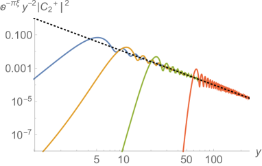
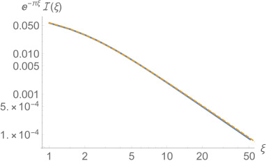
Figure 6: (Left panel) The integrand of $\mathcal{I}(\xi)$ defined in eq. (4.7) normalized by $e^{-\pi\xi}$ is plotted for $\xi=1$ (blue), $4$ (orange), 10 (green) and 30 (red). The black dashed line denotes $y^{-2}$. We fix $n=3$. (Right panel) The comparison between the numerical integration of $e^{-\pi\xi}\mathcal{I}(\xi)$ (blue thick line) and our fit in eq. (4.7) (orange dashed line). The relative error is within $3\%$ up to $\xi=12$.

To calculate the energy fraction of the electromagnetic fields $\Omega_{\rm em}$, we need to numerically evaluate $\mathcal{I}(\xi)$ defined in eq. (4.7). Since we know the asymptotic behavior $|C_{2}^{+}(y)|^{2}=e^{\pi\xi}$ in the limit $y\to\infty$, we are interested in the behavior of $\mathcal{I}(\xi)/e^{\pi\xi}$. In the left panel of fig. 6, the integrand of $\mathcal{I}(\xi)$ normalized by $e^{-\pi\xi}$ is shown. One can see that $e^{-\pi\xi}|C_{2}^{+}|^{2}$ reaches $y^{-2}$ around $y\simeq 2\xi+3$ in the case of $n=3$. Approximating $|C_{2}^{+}(y)|^{2}$ by $e^{\pi\xi}\theta(y-2\xi-3)$ with $\theta(y)$ being the Heaviside function, we obtain

$$\int_{0}^{\infty}\frac{\mathrm{d}y}{y^{3}}\,\left|C^{+}_{2}(y)\right|^{2}\sim e^{\pi\xi}\int_{2\xi+3}^{\infty}\frac{\mathrm{d}y}{y^{3}}=\frac{e^{\pi\xi}}{2(2\xi+3)^{2}}.$$ (B.1)

This expression incentivizes us to fit our numerical result by $e^{\pi\xi}/(\alpha\xi^{2}+\beta\xi+\gamma)$ in eq. (4.7). We find $\alpha\approx 4.7,\ \beta\approx 2.7,\ \gamma\approx 10$ and this fit is compared with the numerical integration in the right panel of fig. 6.

The reason why $y\equiv-k\eta_{i}\simeq 2\xi$ is a threshold can be seen in eq. (2.12). At $-k\eta_{i}=2\xi$, the sign of $k^{2}+2\xi k/\eta_{i}$ flips, and hence the $(+)$-helicity mode gets destabilized and amplified. As $\xi$ is larger, the lowest $k$-mode which becomes unstable at $\eta=\eta_{i}$ becomes higher. It pushes the IR cutoff to a higher $k$-mode (i.e. smaller scale). Therefore $\Omega_{\rm em}$ mainly contributed by the IR cutoff mode relatively decreases as $\xi$ increases, while the amplitude of the scale-invariant part of $\mathcal{P}_{B}^{\rm now}$ does not change.

References

- [1] M. L. Bernet, F. Miniati, S. J. Lilly, P. P. Kronberg and M. Dessauges-Zavadsky, Nature 454 (2008) 302 doi:10.1038/nature07105 [arXiv:0807.3347 [astro-ph]].
- [2] A. Bonafede, L. Feretti, M. Murgia, F. Govoni, G. Giovannini, D. Dallacasa, K. Dolag and G. B. Taylor, Astron. Astrophys. 513 (2010) A30 doi:10.1051/0004-6361/200913696 [arXiv:1002.0594 [astro-ph.CO]].
- [3] L. Feretti, G. Giovannini, F. Govoni and M. Murgia, Astron. Astrophys. Rev. 20 (2012) 54 doi:10.1007/s00159-012-0054-z [arXiv:1205.1919 [astro-ph.CO]].
- [4] A. Neronov and I. Vovk, Science 328 (2010) 73 doi:10.1126/science.1184192 [arXiv:1006.3504 [astro-ph.HE]].
- [5] K. Dolag, M. Kachelriess, S. Ostapchenko and R. Tomas, Astrophys. J. 727 (2011) L4 doi:10.1088/2041-8205/727/1/L4 [arXiv:1009.1782 [astro-ph.HE]].
- [6] W. Essey, S. Ando and A. Kusenko, Astropart. Phys. 35 (2011) 135 doi:10.1016/j.astropartphys.2011.06.010 [arXiv:1012.5313 [astro-ph.HE]].
- [7] A. M. Taylor, I. Vovk and A. Neronov, Astron. Astrophys. 529 (2011) A144 doi:10.1051/0004-6361/201116441 [arXiv:1101.0932 [astro-ph.HE]].
- [8] W. Chen, J. H. Buckley and F. Ferrer, Phys. Rev. Lett. 115 (2015) 211103 doi:10.1103/PhysRevLett.115.211103 [arXiv:1410.7717 [astro-ph.HE]].
- [9] J. D. Finke, L. C. Reyes, M. Georganopoulos, K. Reynolds, M. Ajello, S. J. Fegan and K. McCann, Astrophys. J. 814 (2015) no.1, 20 doi:10.1088/0004-637X/814/1/20 [arXiv:1510.02485 [astro-ph.HE]].
- [10] M. Ackermann et al. [Fermi-LAT Collaboration], Astrophys. J. Suppl. 237 (2018) no.2, 32 doi:10.3847/1538-4365/aacdf7 [arXiv:1804.08035 [astro-ph.HE]].
- [11] P. A. R. Ade et al. [Planck Collaboration], Astron. Astrophys. 594 (2016) A19 doi:10.1051/0004-6361/201525821 [arXiv:1502.01594 [astro-ph.CO]].
- [12] H. Tashiro and T. Vachaspati, Phys. Rev. D 87 (2013) no.12, 123527 doi:10.1103/PhysRevD.87.123527 [arXiv:1305.0181 [astro-ph.CO]].
- [13] H. Tashiro, W. Chen, F. Ferrer and T. Vachaspati, Mon. Not. Roy. Astron. Soc. 445 (2014) no.1, L41 doi:10.1093/mnrasl/slu134 [arXiv:1310.4826 [astro-ph.CO]].
- [14] W. Chen, B. D. Chowdhury, F. Ferrer, H. Tashiro and T. Vachaspati, Mon. Not. Roy. Astron. Soc. 450 (2015) no.4, 3371 doi:10.1093/mnras/stv308 [arXiv:1412.3171 [astro-ph.CO]].
- [15] R. Durrer and A. Neronov, Astron. Astrophys. Rev. 21 (2013) 62 doi:10.1007/s00159-013-0062-7 [arXiv:1303.7121 [astro-ph.CO]].
- [16] K. Subramanian, Rept. Prog. Phys. 79 (2016) no.7, 076901 doi:10.1088/0034-4885/79/7/076901 [arXiv:1504.02311 [astro-ph.CO]].
- [17] B. Ratra, Astrophys. J. 391 (1992) L1. doi:10.1086/186384
- [18] M. Gasperini, M. Giovannini and G. Veneziano, Phys. Rev. Lett. 75 (1995) 3796 doi:10.1103/PhysRevLett.75.3796 [hep-th/9504083].
- [19] V. Demozzi, V. Mukhanov and H. Rubinstein, JCAP 0908 (2009) 025 doi:10.1088/1475-7516/2009/08/025 [arXiv:0907.1030 [astro-ph.CO]].
- [20] T. Fujita and S. Mukohyama, JCAP 1210 (2012) 034 doi:10.1088/1475-7516/2012/10/034 [arXiv:1205.5031 [astro-ph.CO]].
- [21] K. Bamba and J. Yokoyama, Phys. Rev. D 69 (2004) 043507 doi:10.1103/PhysRevD.69.043507 [astro-ph/0310824].
- [22] S. Kanno, J. Soda and M. a. Watanabe, JCAP 0912 (2009) 009 doi:10.1088/1475-7516/2009/12/009 [arXiv:0908.3509 [astro-ph.CO]].
- [23] N. Barnaby, R. Namba and M. Peloso, Phys. Rev. D 85 (2012) 123523 doi:10.1103/PhysRevD.85.123523 [arXiv:1202.1469 [astro-ph.CO]].
- [24] M. Giovannini, Phys. Rev. D 87 (2013) no.8, 083004 doi:10.1103/PhysRevD.87.083004 [arXiv:1302.2243 [hep-th]].
- [25] T. Fujita and S. Yokoyama, JCAP 1309 (2013) 009 doi:10.1088/1475-7516/2013/09/009 [arXiv:1306.2992 [astro-ph.CO]].
- [26] T. Fujita and S. Yokoyama, JCAP 1403 (2014) 013 Erratum: [JCAP 1405 (2014) E02] doi:10.1088/1475-7516/2014/03/013, 10.1088/1475-7516/2014/05/E02 [arXiv:1402.0596 [astro-ph.CO]].
- [27] R. J. Z. Ferreira, R. K. Jain and M. S. Sloth, JCAP 1310 (2013) 004 doi:10.1088/1475-7516/2013/10/004 [arXiv:1305.7151 [astro-ph.CO]].
- [28] R. J. Z. Ferreira, R. K. Jain and M. S. Sloth, JCAP 1406 (2014) 053 doi:10.1088/1475-7516/2014/06/053 [arXiv:1403.5516 [astro-ph.CO]].
- [29] T. Kobayashi, JCAP 1405 (2014) 040 doi:10.1088/1475-7516/2014/05/040 [arXiv:1403.5168 [astro-ph.CO]].
- [30] T. Fujita and R. Namba, Phys. Rev. D 94 (2016) no.4, 043523 doi:10.1103/PhysRevD.94.043523 [arXiv:1602.05673 [astro-ph.CO]].
- [31] M. S. Turner and L. M. Widrow, Phys. Rev. D 37 (1988) 2743. doi:10.1103/PhysRevD.37.2743
- [32] W. D. Garretson, G. B. Field and S. M. Carroll, Phys. Rev. D 46 (1992) 5346 doi:10.1103/PhysRevD.46.5346 [hep-ph/9209238].
- [33] G. B. Field and S. M. Carroll, Phys. Rev. D 62 (2000) 103008 doi:10.1103/PhysRevD.62.103008 [astro-ph/9811206].
- [34] R. Durrer, L. Hollenstein and R. K. Jain, JCAP 1103 (2011) 037 doi:10.1088/1475-7516/2011/03/037 [arXiv:1005.5322 [astro-ph.CO]].
- [35] M. M. Anber and L. Sorbo, JCAP 0610 (2006) 018 doi:10.1088/1475-7516/2006/10/018 [astro-ph/0606534].
- [36] T. Fujita, R. Namba, Y. Tada, N. Takeda and H. Tashiro, JCAP 1505 (2015) no.05, 054 doi:10.1088/1475-7516/2015/05/054 [arXiv:1503.05802 [astro-ph.CO]].
- [37] P. Adshead, J. T. Giblin, T. R. Scully and E. I. Sfakianakis, JCAP 1610 (2016) 039 doi:10.1088/1475-7516/2016/10/039 [arXiv:1606.08474 [astro-ph.CO]].
- [38] D. T. Son, Phys. Rev. D 59 (1999) 063008 doi:10.1103/PhysRevD.59.063008 [hep-ph/9803412].
- [39] M. Christensson, M. Hindmarsh and A. Brandenburg, Phys. Rev. E 64 (2001) 056405 doi:10.1103/PhysRevE.64.056405 [astro-ph/0011321].
- [40] T. Kahniashvili, A. G. Tevzadze, A. Brandenburg and A. Neronov, Phys. Rev. D 87 (2013) no.8, 083007 doi:10.1103/PhysRevD.87.083007 [arXiv:1212.0596 [astro-ph.CO]].
- [41] C. Caprini and L. Sorbo, JCAP 1410 (2014) no.10, 056 doi:10.1088/1475-7516/2014/10/056 [arXiv:1407.2809 [astro-ph.CO]].
- [42] C. Caprini, M. C. Guzzetti and L. Sorbo, Class. Quant. Grav. 35 (2018) no.12, 124003 doi:10.1088/1361-6382/aac143 [arXiv:1707.09750 [astro-ph.CO]].
- [43] J. Martin and J. Yokoyama, JCAP 0801 (2008) 025 doi:10.1088/1475-7516/2008/01/025 [arXiv:0711.4307 [astro-ph]].
- [44] M. Abramowitz and I. Stegun, ”Handbook of Mathematical Functions”, Dover Publications, New York (1972).
- [45] T. Kobayashi and M. S. Sloth, arXiv:1903.02561 [astro-ph.CO].
- [46] G. Baym and H. Heiselberg, Phys. Rev. D 56 (1997) 5254 doi:10.1103/PhysRevD.56.5254 [astro-ph/9704214].
- [47] E. W. Kolb and M. S. Turner, Front. Phys. 69 (1990) 1.
- [48] A. Brandenburg, J. Schober, I. Rogachevskii, T. Kahniashvili, A. Boyarsky, J. Fröhlich, O. Ruchayskiy and N. Kleeorin, Astrophys. J. 845 (2017) no.2, L21 doi:10.3847/2041-8213/aa855d [arXiv:1707.03385 [astro-ph.CO]].
- [49] T. Kahniashvili, A. Brandenburg, R. Durrer, A. G. Tevzadze and W. Yin, JCAP 1712 (2017) no.12, 002 doi:10.1088/1475-7516/2017/12/002 [arXiv:1610.03139 [astro-ph.CO]].
- [50] R. Banerjee and K. Jedamzik, Phys. Rev. D 70 (2004) 123003 doi:10.1103/PhysRevD.70.123003 [astro-ph/0410032].
- [51] C. Caprini, R. Durrer and E. Fenu, JCAP 0911 (2009) 001 doi:10.1088/1475-7516/2009/11/001 [arXiv:0906.4976 [astro-ph.CO]].
- [52] J. S. Schwinger, Phys. Rev. 82 (1951) 664. doi:10.1103/PhysRev.82.664
- [53] M. B. Fröb, J. Garriga, S. Kanno, M. Sasaki, J. Soda, T. Tanaka and A. Vilenkin, JCAP 1404 (2014) 009 doi:10.1088/1475-7516/2014/04/009 [arXiv:1401.4137 [hep-th]].
- [54] T. Kobayashi and N. Afshordi, JHEP 1410 (2014) 166 doi:10.1007/JHEP10(2014)166 [arXiv:1408.4141 [hep-th]].
- [55] T. Hayashinaka, T. Fujita and J. Yokoyama, JCAP 1607 (2016) no.07, 010 doi:10.1088/1475-7516/2016/07/010 [arXiv:1603.04165 [hep-th]].
- [56] H. Kitamoto, Phys. Rev. D 98 (2018) no.10, 103512 doi:10.1103/PhysRevD.98.103512 [arXiv:1807.03753 [hep-th]].
- [57] O. O. Sobol, E. V. Gorbar, M. Kamarpour and S. I. Vilchinskii, Phys. Rev. D 98 (2018) no.6, 063534 doi:10.1103/PhysRevD.98.063534 [arXiv:1807.09851 [hep-ph]].
- [58] M. Banyeres, G. Domènech and J. Garriga, JCAP 1810 (2018) no.10, 023 doi:10.1088/1475-7516/2018/10/023 [arXiv:1809.08977 [hep-th]].
- [59] V. Domcke and K. Mukaida, JCAP 1811 (2018) no.11, 020 doi:10.1088/1475-7516/2018/11/020 [arXiv:1806.08769 [hep-ph]].
- [60] K. Fukushima, D. E. Kharzeev and H. J. Warringa, Phys. Rev. D 78 (2008) 074033 doi:10.1103/PhysRevD.78.074033 [arXiv:0808.3382 [hep-ph]].
- [61] A. Boyarsky, J. Fröhlich and O. Ruchayskiy, Phys. Rev. Lett. 108 (2012) 031301 doi:10.1103/PhysRevLett.108.031301 [arXiv:1109.3350 [astro-ph.CO]].
- [62] Y. Akamatsu and N. Yamamoto, Phys. Rev. Lett. 111 (2013) 052002 doi:10.1103/PhysRevLett.111.052002 [arXiv:1302.2125 [nucl-th]].
- [63] J. Schober, I. Rogachevskii, A. Brandenburg, A. Boyarsky, J. Fröhlich, O. Ruchayskiy and N. Kleeorin, Astrophys. J. 858 (2018) no.2, 124 doi:10.3847/1538-4357/aaba75 [arXiv:1711.09733 [physics.flu-dyn]].
- [64] J. Schober, A. Brandenburg, I. Rogachevskii and N. Kleeorin, arXiv:1803.06350 [physics.flu-dyn].
- [65] P. Adshead, L. Pearce, M. Peloso, M. A. Roberts and L. Sorbo, JCAP 1806 (2018) no.06, 020 doi:10.1088/1475-7516/2018/06/020 [arXiv:1803.04501 [astro-ph.CO]].
- [66] M. Giovannini and M. E. Shaposhnikov, Phys. Rev. D 57 (1998) 2186 doi:10.1103/PhysRevD.57.2186 [hep-ph/9710234].
- [67] T. Fujita and K. Kamada, Phys. Rev. D 93 (2016) no.8, 083520 doi:10.1103/PhysRevD.93.083520 [arXiv:1602.02109 [hep-ph]].
- [68] K. Kamada and A. J. Long, Phys. Rev. D 94 (2016) no.6, 063501 doi:10.1103/PhysRevD.94.063501 [arXiv:1606.08891 [astro-ph.CO]].
- [69] K. Kamada and A. J. Long, Phys. Rev. D 94 (2016) no.12, 123509 doi:10.1103/PhysRevD.94.123509 [arXiv:1610.03074 [hep-ph]].
- [70] D. Jiménez, K. Kamada, K. Schmitz and X. J. Xu, JCAP 1712 (2017) no.12, 011 doi:10.1088/1475-7516/2017/12/011 [arXiv:1707.07943 [hep-ph]].
- [71] K. Kamada, Phys. Rev. D 97 (2018) no.10, 103506 doi:10.1103/PhysRevD.97.103506 [arXiv:1802.03055 [hep-ph]].
- [72] C. Caprini, R. Durrer and G. Servant, JCAP 0912 (2009) 024 doi:10.1088/1475-7516/2009/12/024 [arXiv:0909.0622 [astro-ph.CO]].