Bayesian Search for Robust Optima
Abstract.
Many expensive black-box optimisation problems are sensitive to their inputs. In these problems it makes more sense to locate a region of good designs, than a single—possibly fragile—optimal design.
Expensive black-box functions can be optimised effectively with Bayesian optimisation, where a Gaussian process is a popular choice as a prior over the expensive function. We propose a method for robust optimisation using Bayesian optimisation to find a region of design space in which the expensive function’s performance is relatively insensitive to the inputs whilst retaining a good quality. This is achieved by sampling realisations from a Gaussian process that is modelling the expensive function, and evaluating the improvement for each realisation. The expectation of these improvements can be optimised cheaply with an evolutionary algorithm to determine the next location at which to evaluate the expensive function. We describe an efficient process to locate the optimum expected improvement. We show empirically that evaluating the expensive function at the location in the candidate uncertainty region about which the model is most uncertain, or at random, yield the best convergence in contrast to exploitative schemes.
We illustrate our method on six test functions in two, five, and ten dimensions, and demonstrate that it is able to outperform two state-of-the-art approaches from the literature. We also demonstrate our method one two real-world problems in 4 and 8 dimensions, which involve training robot arms to push objects onto targets.
1. Introduction
Optimisation is the search for the best-performing design with respect to a predefined objective function. In an ideal scenario the objective function would be well behaved and insensitive to small changes in the design parameters. Any loss of performance due to the mis-specification of the parameters or the inaccuracy of the model itself would be negligible and largely go unnoticed. But, for most real-world problems this is not the case. Often the landscape of real objective functions varies rapidly as the design parameters change, so even a small perturbation to these parameters could lead to an unacceptably diminished performance. Such perturbations are frequently the manifestation of uncertainties in the design process, and arise for a number of reasons. For example: tolerances in the manufacturing process may mean that the realised design is slightly different from the modelled one; once the design has been produced it may be operated away from its design conditions; the model used to optimise the design may not accurately reflect reality; or there may be uncertainties in the environmental conditions (e.g. air temperature or pressure).
The goal of robust optimisation is to locate the best designs that have stable performance irrespective of small perturbations to the design parameters. Classic global optimisers are often ineffective at solving this problem, because robust optima do not necessarily coincide with global optima; in fact optimal robust designs potentially exist in a different region of the domain altogether!
A straightforward way to quantify the robustness of a proposed optimum is to evaluate the objective function for a large number of design parameters in the vicinity of the optimum. However, this strategy is ineffective when the objective function is expensive to evaluate. These expensive-to-evaluate functions are common to many disciplines, including tuning the parameters of machine learning algorithms (Bergstra et al., 2011; Snoek et al., 2012), robotics (Tesch et al., 2011; Lizotte et al., 2007), and other engineering design problems (Daniels et al., 2018; Anthony and Keane, 2003; Wiesmann et al., 1998; Volz et al., 2019; Shourangiz-Haghighi et al., 2020). Bayesian optimisation is a principled and efficient technique for the global optimisation of these sorts of functions. The idea underlying Bayesian optimisation is to place a prior distribution over the objective function and then update that prior with observations of the objective function (obtained by expensively evaluating it) in order to yield a posterior predictive distribution. This posterior distribution thus encodes the optimiser’s knowledge of the objective function landscape. It is then used to inform where to make the next observation of the objective function through the use of an acquisition function, which balances the exploitation of regions known to have good performance with the exploration of regions where there is little information about the function’s response. A Gaussian process is a popular choice of prior, because they are intuitive to understand, capable of modelling the objective function accurately with few data, and cheap to evaluate.
The chief contribution of this paper is the introduction of a novel acquisition function for the Bayesian robust optimisation of expensive black-box functions. Although we have phrased robust optimisation as seeking an optimum robust to “small perturbations” of design parameters, the technique we present is applicable to arbitrarily large perturbations. We evaluate the method on 6 benchmark functions and a real-world problem showing that it provides state-of-the-art performance compared with two competing algorithms.
We begin by outlining background material and reviewing similar techniques in Section 2. Section 3 builds upon the previous section by introducing the Bayesian optimisation of the robust domain, and giving a demonstration on a toy function in one dimension. Results of five- and ten-dimensional test problems are presented alongside analysis in Section 4, where we also evaluate the algorithms on two active learning robot pushing problems. Finally, the conclusion and suggestions for future work can be found in Section 5.
2. Background
This section comprises background material in Bayesian optimisation (Section 2.1), Gaussian processes (Section 2.2), and robust optimisation for expensive-to-evaluate functions (Section 2.3).
2.1. Bayesian optimisation
Although stochastic search algorithms, such as evolutionary algorithms, have been popular for the optimisation of black-box functions, Bayesian optimisation is often more attractive, particularly for expensive-to-evaluate functions. Through explicitly modelling the expensive function and accounting for the uncertainty in the model, the search can be guided efficiently to promising areas of the decision space: either those with high certainty of being better than the current best solution, or those with high uncertainty that may be better than the current best. See (Brochu et al., 2010) for an introduction to Bayesian optimisation, and (Shahriari et al., 2016) for a recent comprehensive review.
To be definite and without loss of generality, we assume that the goal of optimisation is to minimise a function , where are the design parameters in the feasible space .
Bayesian optimisation relies on constructing a probabilistic model of . Assume that has been (expensively) evaluated at locations so that data are available from which to learn a model. Then Bayesian modelling is used to construct a posterior predictive distribution at any desired location . Crucially, Bayesian modelling gives not only a prediction of the function value at , but the posterior distribution quantifies the uncertainty in the prediction as well. Where next to expensively evaluate in is determined by an acquisition function, which balances the exploitation of predicted good values of with exploring uncertain and potentially good regions. Here we use the popular expected improvement (Jones et al., 1998), which has been shown to be effective in practice and for which some theoretical guarantees exist (Bull, 2011). Alternatives such as the probability of improvement (Kushner, 1964) or upper-confidence bound (Srinivas et al., 2010; Brochu et al., 2010) could also be used.
If is modelled to take the value , then the improvement at is defined as
| (1) |
where
| (2) |
is the best function value from the evaluations thus far. The expected improvement is then
| (3) |
Gaussian processes are commonly used for modelling in which case the posterior predictive distribution is itself a Gaussian density (see Section 2.2) with mean and variance . In this case the expected improvement has the closed analytical form (Jones et al., 1998):
| (4) |
where and and are the standard Normal density and cumulative distribution functions respectively.
The next (expensive) evaluation is then chosen as that with the greatest expected improvement: . This location is often discovered by using an evolutionary algorithm to maximise , which is rapid since is computationally cheap to evaluate. The evaluated location and its function value are added to and the optimisation proceeds iteratively until some stopping criterion is met or, more commonly, the available computational resources are exhausted.
2.2. Gaussian processes
Gaussian processes (GPs) (Rasmussen and Williams, 2006) are commonly used for Bayesian optimisation due to their flexibility and the simple Gaussian predictive posterior distributions. Briefly, a GP is a collection of random variables, and any finite number of these have a joint Gaussian distribution. Given data and a feature vector , the GP posterior predictive density of the target is Gaussian:
| (5) |
where the mean and variance of the prediction are given by
| (6) | ||||
| (7) |
Here is the vector of evaluated function values at . Non-linearity in the GP enters through a kernel function which models the covariance between two feature vectors. The covariance matrix collects these covariances together, , and is the -dimensional vector of covariances between the training data and : . There are a number of kernels that could be used, for example the squared exponential function or the Matérn family of covariance functions (Rasmussen and Williams, 2006); here we used the Matérn covariance function with smoothing parameter which has been recommended for modelling realistic functions (Snoek et al., 2012).
In addition the kernel function depends upon a number of hyper-parameters, . Training the GP comprises inferring these hyper-parameters by maximising the marginal likelihood of the data given by
| (8) |
Although the log marginal likelihood function landscape may be non-convex and multi-modal, we adopt the standard practice of using a gradient-based optimiser (L-BFGS) with several random starts to estimate good hyper-parameter values (GPy, 2012).
2.3. Robust Optimisation of Expensive Functions
The focus of robust optimisation is to determine function optima in the face of uncertainty. These uncertainties are typically considered to arise in one of three categories: (a) design uncertainties, (b) model uncertainties, or (c) environmental uncertainties (Beyer and Sendhoff, 2007). A variety of methods exist to alleviate the added complexity of searching for robust optima; comprehensive surveys are given by Beyer and Sendhoff (2007) and Gabrel et al. (2014).
In this work we focus on one category of robustness: uncertainties or mis-specification in the design parameters. In this case robust optimisation seeks to find an where some small perturbation does not cause the objective function’s response at to become unacceptably poor. We define the set of all possible perturbations to be
| (9) |
where is the robustness parameter, and is a function controlling the shape of the robust region, which is often a distance function. The choice of and is determined by the problem owner.
A quality function can be used to quantify the robustness of . There are a number of ways one could formulate , for example the average performance over the perturbations:
| (10) |
where denotes the probability that in practice will be evaluated at rather than . Although for analytic convenience is sometimes taken to be unbounded and is taken to be a Gaussian distribution centred on , in most real applications is taken to be a (small) compact set and is uniform on it.
An alternative quality function, which may be more useful in practice, is to guarantee the worst-case performance (Beyer and Sendhoff, 2007),
| (11) |
Having defined a quality function, robustness parameter, and shape function the robust optimisation problem may be written as:
| (12) |
Here we further assume that the objective function is a computationally-expensive-to-evaluate black box. For a general review of robust optimisation with expensive functions see (Chatterjee et al., 2019). When the objective function is expensive to evaluate, optimisers such as evolutionary algorithms (Branke, 1998; Paenke et al., 2006) or particle swarm optimisation (Dippel, 2010) will not be viable due to the large number of function evaluations they demand. Therefore it is essential to apply methods that necessitate only small numbers of observations. In spite of this requirement, relatively few methods exist in the literature to address this problem (Chatterjee et al., 2019).
A related field is that of level set estimation (Gotovos et al., 2013), where the aim is to determine a set of points of equal objective function value, which encompass a region where the performance is guaranteed to be better than some given threshold (either as a specific value or percentage of the unknown optimum). Bogunovic et al. (2016) extended the idea of level set estimation to work in a unified fashion with Bayesian optimisation.
There are a few methods in the literature that use GPs to develop a surrogate model of the expensive function (Jin, 2011; Ong et al., 2006; Lee and Park, 2006), which reduces the computational cost of the optimisation in two ways. Firstly, it enables the surrogate model (rather than the expensive function) to be searched using, for example, an evolutionary algorithm or simulated annealing. Secondly, the use of a surrogate has the clear benefit of curtailing the computational burden of evaluating the robustness of solutions, because the surrogate model can be interrogated instead of the true objective function. Although these methods lighten the computational load, they do not take advantage of the uncertainty in the surrogate model, which is available when using a GP and could be used to help guide the search in subsequent iterations. Picheny et al. (2013) present a review of robust acquisition functions for use with a GP, but these only account for noise in the function’s response.
A state-of-the-art Bayesian approach was presented by ur Rehman et al. (2014). This method exploits a GP with a modified formulation of the expected improvement, which aims to account for the robust performance over a region of the design space. Whilst this technique is shown to be useful for expensive robust optimisation, there are two drawbacks: (a) the uncertainty of the GP is largely disregarded when calculating the modified expected improvement, as only the uncertainty at the estimated worst performing location is considered; and (b) this method is demonstrated with a somewhat substantial number of initial observations (100 in 10 dimensions), which makes it rather unsuitable for very expensive functions. Since this method is considered to be state-of-the-art we have elected to include our own implementation of it for comparison during experimentation.
More recently the StableOpt algorithm has been presented (Bogunovic et al., 2018). This is a confidence-bounds approach that exploits a Gaussian process model to locate a region of good inputs. In essence, at each time-step , a candidate robust location is found as
| (13) |
where denotes the lower confidence bound acquisition function:
| (14) |
where and are the posterior predictive mean and variance at (equations (6) and (7)). Adding to instead of subtracting it obtains the upper confidence bound function, . After identifying a candidate robust location, an expensive evaluation is made at the location such that
| (15) |
Performing the search in this way ensures that the search operates pessimistically when identifying robust optima, yet optimistically when determining the next location at which to evaluate the expensive function.
3. Bayesian Search for a Robust Optimum
The search for a robust optimum can be distilled to the minimisation of the selected quality function (Section 2.3) for a given robust set . The obstacle to straightforward optimisation is that evaluating for any candidate location is unachievable for continuous domains, because the evaluation of is required for all . In spite of this, one can envisage that a good approximation to could be made by aggregating over many . Although such an approach is practicable for cheap-to-evaluate objective functions, the need to optimise expensive functions renders this approximation infeasible as well.
Here we propose to search for the robust optimum by constructing a Gaussian process model of the expensive function , and then using it to estimate the chosen quality function to determine the robust quality at a particular location. This allows approximation of the expected improvement for candidate locations by drawing realisations from the Gaussian process and then evaluating the improvement for each realisation based on these estimated quality values. Algorithm 1 shows the main steps in our robust optimisation procedure.
Inputs
:
Initial observation locations
:
Expensive evaluations
:
Sampling function
(Section 3.2)
:
Template of locations covering a robust set
:
Function approximating quality of a set of function
evaluations
:
Number of realisations to draw from GP
Procedure
The process is initialised with a small number of evaluations of , usually chosen using a low discrepancy sampling scheme (Matoušek, 1998), such as a Sobol’ sequence (Sobol’, 1967) or Latin hypercube sampling (Morris and Mitchell, 1995; McKay et al., 1979). These allow a Gaussian process to be constructed (line 2).
In Algorithm 1 we make use of a template which is a discretised representation of the robust set . The exact structure of is left to the practitioner, but there are several considerations for constructing a template that would be useful in practice. Firstly the set of points constituting the template could be distributed uniformly within the bounds of the robust set, alternatively it would be possible to arrange the set of points to be more densely distributed near the centre of the robust set, thus giving greater weight to perturbations closer to the centre of the robust set; cf equation (10). Finally, for worst case performance guarantees (equation (11)) one might consider placing a larger proportion of points on the boundary of the robust set, because this is where one might assume the extremes of the function response within the robust set would be.
Next, an appropriate quality function (Section 2.3) must be selected to estimate the robust quality of a location. Again, the choice of this function is left to the practitioner, but here we provide two such examples of modified quality functions which operate on sets of response values for each location within the robust set template. Denoting the set of responses estimated from the GP surrogate by , worst-case quality function is estimated as
| (16) |
and the average quality function by
| (17) |
Over lines 12 to 18 of Algorithm 1, a realisation is drawn from the fitted Gaussian process model for the set of that constitute the candidate and best-so-far templates for the robust region ( and respectively). Note that a realisation evaluated at a set of locations is a draw from a multivariate Gaussian where . Then the improvement for each realisation can be calculated as per line 16 and the expected improvement is the mean of the realisation-specific improvements (line 19).
Ordinarily, in non-robust Bayesian optimisation, the best returned location is one of the observations , which provides some guarantee about the quality of the returned location. In order to provide a similar guarantee we suggest that it is reasonable to enforce that the returned best robust location should be within the vicinity of at least one expensively evaluated location, that is for to be considered a valid solution there must exist such that , where is the set of evaluated locations, and and are the distance function and robustness parameter defining the robust set (9). For convenience we write
| (18) |
for the robust set located at . Then the requirement that the robust optimum should be near an evaluated location means that the set of possible locations for the best robust optimum found so far is , which is illustrated in Figure 4. With expensively evaluated locations , the best robust location is identified as:
| (19) |
and can be found using, for example, an evolutionary optimiser to search over the (Algorithm 1 line 3). We discuss the computation of in more detail in Section 3.3.
As we show below, although we demand that a robust location is within the vicinity of an evaluated location, it can be advantageous to evaluate at a location other than that with maximum expected improvement. In Section 3.2 we explore a number of criteria for choosing the location to evaluate. In Algorithm 1 is expensively evaluated at the location provided by the function (lines 5 and 7). This sequence is then repeated until convergence is achieved or computational resources are exhausted.
We now illustrate the full procedure with a toy example.
3.1. Toy Example
We illustrate the procedure using the toy one-dimensional function
| (20) |
for . For simplicity we restrict the robust set to be an interval, where the robustness parameter defines the span of the interval, and the shape function is given by , where .
Figure 1a shows the toy target function and the induced robust landscape for the worst-case quality as given by (11). This toy function illustrates how the optimal single point location, namely the minimum of , can exist in a distinct location from the optimal robust region.
The first step is to fit a Gaussian process to an initial set of observations of the expensive function . In this instance we have used an initial set of observations; example draws from the resulting Gaussian process can be seen in Figure 1b.
Each realisation of the Gaussian process can be thought of as a potential whose quality can be evaluated using the chosen quality function. Figure 1c shows the result of applying the quality function to a drawn realisation together with the resulting improvement from that realisation.
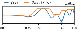
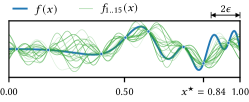
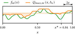
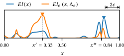
For simplicity in this example, we have constrained the best uncertainty set to be centred on an observation ; the best uncertainty set so far (for the depicted realisation) is centred at , including the observation at . The robust quality for each realisation is calculated as the difference between the robust quality of the best-so-far location and the candidate location; as shown in Algorithm 1 on line 16 and the robust expected improvement is approximated as an average over all of the realisations, using the procedure given between lines 10 and 19 of Algorithm 1. This is the acquisition function used for determining where to sample next. Figure 1 (bottom) compares the robust expected improvement with the (usual) single-point expected improvement (4), which clearly demonstrates that the robust expected improvement gives greater weight to searching the more robust regions of design space.

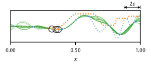
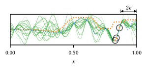
Figure 2 shows the result of continuing the optimisation procedure for three additional iterations; the objective function is evaluated at the location of maximum expected improvement, . The robust optimiser quickly locates the region of the robust optimum, whereas the single-point optimiser searches the region of the (fragile) global minimum.
3.2. Sampling Location
Non-robust acquisition functions, such as the expected improvement described in Section 2.1, determine a point of maximum acquisition. In contrast, their robust counterparts yield a region, which presents an additional decision in the optimisation process: where within this region should the next observation of the target function be made?
We constrain the location of the new observation to be within the robust set of maximum acquisition . Further, we propose the use of a sampling function , which determines where within to locate the next expensive evaluation: . As we show empirically in section 4 on a range of test functions, the choice of has a significant impact on the algorithm’s ability to converge to the best uncertainty region. Here we present five suggestions for the sampling function ; Figure 3 illustrates each of them.

- Centred observation.:
-
Usually uncertainty sets are symmetrical about and an obvious choice is to observe the objective function at the location of maximum expected improvement—the centre of the uncertainty set:
(21) - Most uncertain observation.:
-
A maximally explorative approach to improving the estimate of the quality of the predicted best uncertainty set is to observe the expensive function at the location of maximum uncertainty within :
(22) where is the predicted variance of the Gaussian process at , see (7).
- Worst-case prediction.:
-
An alternative to improve the estimate of the uncertainty set’s quality is to query at the location of the worst-case predicted value:
(23) where is the predicted mean of the Gaussian process at . This strategy has the benefit of confirming or revising the predicted worst case performance with an actual evaluation.
- Uniformly at random.:
-
Finally, draw uniformly at random within :
(24) This approach may also be expected to promote exploration, but not in such a directed way as the “most uncertain observation” scheme.
- UCB.:
-
Taking inspiration from StableOpt, we locate such that it maximises the upper confidence bound within the proposed robust region:
(25) where, as with StableOpt, we take .
3.3. Best-So-Far Robust Location
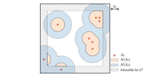
In standard Bayesian optimisation the best-so-far location and its function value are simply available because has been evaluated at all , so deciding on the current is merely a matter of comparing the evaluated locations and then selecting the best one. However, in this robust scheme the improvement for a particular realisation requires a procedure to search for the quality of the best robust region: so that candidate robust centres can be compared with it. Since the evaluation of requires evaluating the modelled at a set of locations covering , this optimisation in turn requires evaluating the modelled over all locations that might be covered by the robust region, that is over the extended neighbourhood of :
| (26) |
The extended neighbourhood is illustrated in Figure 4.
To avoid this potentially expensive optimisation for every draw of a realisation of , we instead identify the best robust region as:
| (27) |
where is evaluated from the mean of the modelled :
| (28) |
As shown in Algorithm 1, is determined once each new observation is acquired (line 4).
By evaluating at a number of locations in a candidate robust set, the improvement for a particular realisation is then evaluated as
| (29) |
with the best quality found so far estimated as:
| (30) |
3.4. Convergence
Essentially we aim to perform Bayesian optimisation on the induced robust landscape (11). As a result all of the usual theoretical guarantees for the convergence of Bayesian optimisation already presented in the literature for Bayesian optimisation apply. In particular Bull (2011) shows that Bayesian optimisers using the expected improvement acquisation function as here converge under certain conditions; see also (Vazquez and Bect, 2010).
However, it should be recognised that there are two points where this algorithm makes approximations that affect guarantees of convergence, which we discuss briefly here.
Firstly, the expected improvement is approximated by averaging over sample realisations drawn from the Gaussian process modelling . In the large sample limit this approximation converges to the desired value, like in the number of realisations . However, in practice the acquisition function is approximated with relatively few samples (up to in the experiments reported here.)
Secondly, we approximate the quality of a robust set by evaluating the Gaussian process at a set of locations over the template covering the robust set (here we use 60 samples in 2 dimensions, 250 samples in 5 dimensions, and 400 samples in 10 dimensions). Clearly, this approximation may under-estimate the worst case quality and it relies on the fidelity of the Gaussian process approximation. Sufficiently dense sampling of can achieve a good approximation and an alternative is to use a search procedure such as direct (Jones et al., 1993) which can provide an upper bound to the worst-case performance. In practice, however, we have found this to be exorbitantly expensive.
4. Evaluation
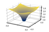
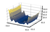
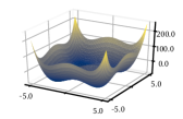
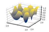
We present results of the performance of our method in comparison to the state-of-the-art methods StableOpt (Bogunovic et al., 2018) and the method described by ur Rehman et al. (2014) with over six common benchmark functions (Mirjalili and Lewis, 2016; Laguna and Martí, 2005; Styblinski and Tang, 1990). We also include some visualisations of results in two dimensions, which serve to demonstrate the differences in search regimes between the compared methods. Figure 5 presents two-dimensional visualisations of each function for reference, which are defined in Table 1.
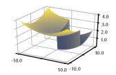
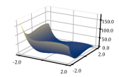
| Name | Equation | |
| Bumped Bowl† (Mirjalili and Lewis, 2016) | ||
| Levy03 (Laguna and Martí, 2005) | ||
| Styblinski-Tang (Styblinski and Tang, 1990) | ||
| Robust Problem 4 (Mirjalili and Lewis, 2016) | ||
| Stepped Sphere† (Mirjalili and Lewis, 2016) | ||
| Quintic (Al-Roomi, 2015) |
Each benchmark was selected to test a different aspect of robust optimisation. Function (Bumped Bowl) presents a situation where the robust optimum is situated at a local maximum, which tests the ability of an algorithm to overlook the better-performing non-robust region. Our implementation of this benchmark has been modified from (Mirjalili and Lewis, 2016) to ensure that the robust optimum exists exactly at the peak of the local maximum. Benchmarks Levy 03 and Mirjalili & Lewis 04 (and ) are examples of functions with multiple local minima. In the case of benchmarks (Styblinkski-Tang) and (Qunitic), the robust optimum resides just outside of the global optimum, which tests robust procedures’ resilience to non-robust regions. Optimisers that exploit the parabolic sphere have difficulty in finding the “step” in (Stepped Sphere) containing the optimum, which occupies a vanishingly small proportion of the domain as the number of dimensions increases. This function has been modified from (Mirjalili and Lewis, 2016) to ensure that the size of the step remains significant as increases: even so, the proportion of containing the lower step is only .



The robust quality measure used for evaluating candidate locations was the worst-case quality (11), the elected shape function was , and the robustness parameter , where and are the upper and lower bounds of the domain respectively (i.e. ). See supplementary material S1.1 and S1.2 for comparative results using a “square-shaped” robust region in 5 and 10 dimensions respectively.
As noted above the functions were modelled with a Gaussian process with a Matérn 5/2 kernel; kernel parameters were inferred by optimising the marginal likelihood (8) using L-BFGS from 10 random restarts. realisations were used in the evaluation of the acquisition function, where increases if no improvement is found at lower values. The location of the acquisition function maximum was found by evaluating it for 1000 Latin hypercube samples and then optimising the most promising 10 of these with L-BFGS-B (Byrd et al., 1995); the optimisation budget was 100 evaluations of the expensive function.
Python code to generate figures and reproduce all experiments is available online111https:github.com/url/completed/on/publication
We evaluated the five sampling schemes proposed in Section 3.2: centred observation (21), most uncertain observation (22), maximised UCB (25), and uniformly at random (24).
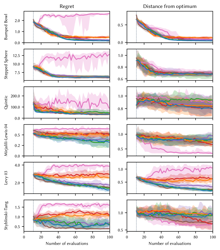
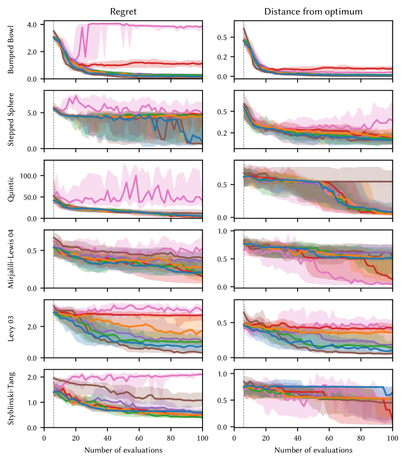
To enable paired comparisons, each method was initialised using the same Latin hypercube samples. The experiments were repeated 30 times for statistical comparison. Figures 6 and 7 compare the convergence of each of the methods tested. For the functions , , and , where it is difficult to analytically determine the robust optimum, we have completed 20 repeated trials of CMA-ES (Hansen et al., 2003) in order to locate an approximation for the global robust optimum.
4.1. Analysis
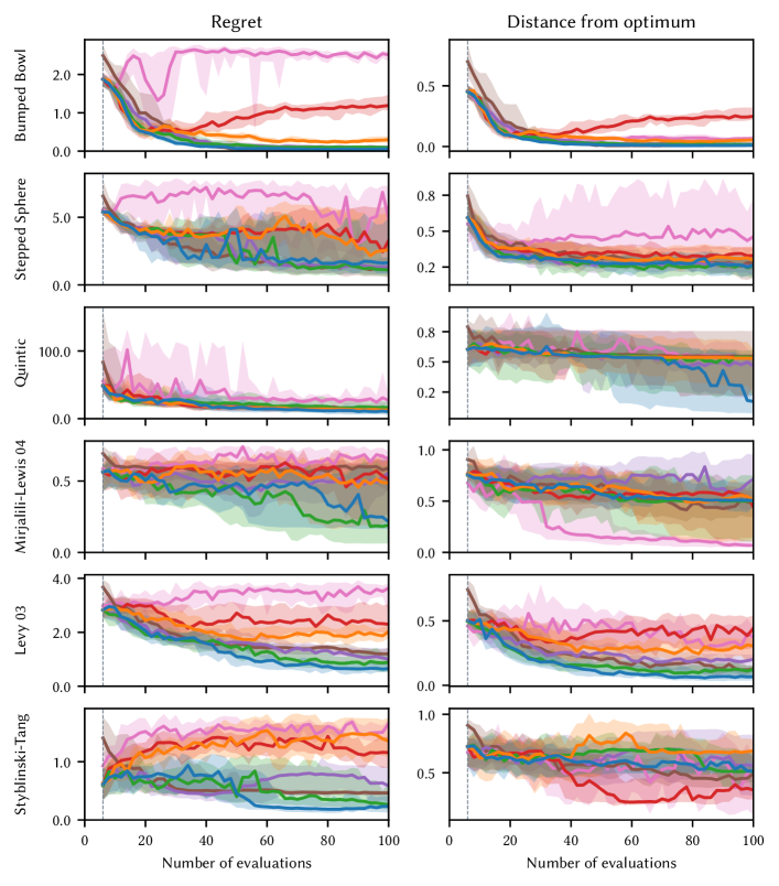
The convergence plots in Figure 6 and Figure 7 show the regret, namely the difference between the state of the optimiser and the value of the true robust minimum. They demonstrate that our robust optimisation procedure is generally capable of locating and exploiting robust optima with a small number of observations of the underlying expensive function. However, we note that all methods perform significantly less well in dimensions and none of the methods are able to locate a good value for the robust optimum for the Levy03 or stepped sphere functions.
A summary of all of the tested algorithms over all of the functions is shown as a critical difference plot (Demšar, 2006) in Figure 8. Of the five competing sampling functions, , sampling at the most uncertain location within the robust region consistently enables better convergence in dimensions. In dimensions the performance of our algorithm with several sampling methods and StableOpt are statistically indistinguishable using the Wilcoxon signed rank test at .


The success of the most uncertain sampling strategy with is largely because of the increased exploration of the best-so-far robust region, which leads to more even coverage of observations in that key region. The benefits of increased exploration are evident for the Stepped Sphere in dimensions where the most uncertain method is the only method of ours that explores the bottom of the parabolic bowl containing the step sufficiently to locate the optimum. In higher dimensions we conjecture that the model of the function is not sufficiently good to allow identification of the most uncertain point.
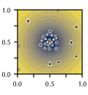
Figure 9 shows the typical search pattern for each of the five sampling methods, StableOpt, and ur Rehman et al.’s approach after 30 iterations on the two-dimensional Bumped Bowl function (Mirjalili and Lewis, 2016). Each run was initialised from the same set of 3 Latin hypercube samples. It is clear from this example that both the “most uncertain” sampling scheme has made a better estimate of the robust optimum. In addition, the “most uncertain” sampling scheme has been exploratory over the remainder of the domain, and has lead to the most even coverage of observations at the robust optimum.
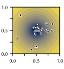
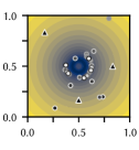
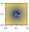
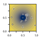
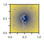
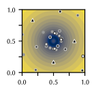
In all of the benchmark functions, our method has out-performed that of ur Rehman et al.’s competing method, with respect to the value of regret at the final iteration. It should be noted that ur Rehman et al.’s method was able to get closer to the optimum location on numerous occasions, but struggled to accurately settle its robust region, which resulted in a much worse value of regret (due to the fragility of the function landscape).
Generally, and as one might expect, the performance of all of the compared schemes worsens as the number of dimensions increases. Benchmark problem is difficult for a GP to model due to the discontinuous downward step in one corner of the domain. This problem is exacerbated in higher dimensions: whilst in two dimensions the downward step covers of the domain, as noted above, the step scales such that it occupies of the domain. The result is that in ten dimensions the downward step exists in less than one-thousandth of the domain. With the extremely limited number of observations made during our experiments it is unsurprising that none of the sampling schemes, StableOpt nor ur Rehman et al.’s method discovered the step. In five dimensions only the “most uncertain” and StableOpt were able to find the step, which indicates that the improved exploration offered by these schemes presents significant advantages in locating complicated response features.
In general ur Rehman et al.’s approach and our approach using the “centre” sampling scheme do not do well, and in fact perform similarly poorly in similar circumstances. This appears to be a result of both of the approaches tending towards making more exploitative observations, which means that they repeatedly sample in approximately the same location and fail to construct an accurate model of .
Each of the presented methods make significant ground towards improving their quality of robustness, as seen in Figures 6 and 7. And each one generally exhibits a similar convergences curve for the initial 20 iterations as the vicinity of the robust optimum is approached. However, during the remainder of the run it is clear that “most uncertain” and “random” generally outperform the other approaches.
4.2. Real-world application

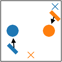
Here we illustrate our robust optimisation method on a real-world problem. We aim to optimise the input parameters for two active learning robot pushing problems (Wang et al., 2018). In the first problem a single robot hand aims to push an object towards an unknown target location; see Figure 10a. Once the robot has pushed the object, per its input parameters, the push is then evaluated as the distance between the target and the final location of the pushed object. The input parameters to this problem are the starting position of the robot hand, the orientation of the robot hand, and the number of time steps for which the robot hand moves. The direction of travel of the robot hand is constrained to be in the direction of the object’s initial location. We refer to this four-dimensional problem as Push4.
In the second problem, as shown in Figure 10b, two robot hands are tasked to push their respective object towards two unknown targets. This problem poses an additional layer of complexity in that both of the robot hands and objects may block each other’s path if they intersect. The resulting feedback from this problem is the sum of the distance between both of the objects and their respective targets. Due to the possibility of the robots and objects blocking each other, some problem instances do not have perfect solutions. There are eight input parameters to optimise in this case: the starting position of both of the robot hands, the orientation of both of the robot hands, and the number of time steps for which each of the robot hands move. The resulting eight-dimensional problem is referred to as Push8.
As with (Wang and Jegelka, 2017), the object’s initial location in Push4 is always at the centre of the domain, but the target location is changed for each of the optimisation runs. Each of the compared algorithms used the same target locations, so that the runs are directly comparable. Doing this means that we average over instances of the problem class, rather than repeatedly optimising the same function from a different set of starting observations. Likewise, in Push8 the starting position of the objects were fixed, and their respective targets were randomised for each optimisation run. In order to estimate the optimum for each of the different initialisations of the problems we initially sampled the feasible space with 1000 different robot parameters, and then locally optimised the landscape using CMA-ES from the best 20 sampled points.
The results of the experiments, shown in Figure 11, show that on the four-dimensional Push4 that the “most uncertain”, “random”, and “centre” selection methods achieve the best median value of regret. However, in eight dimensions all of the selection methods are capable of improving the function value, but there is little to discern between them. In fact all of the selection methods are considered statistically indistinguishable. This is perhaps unsurprising, because the landscape for the Push8 problem is very complicated: there are many plateaux and discontinuities throughout the landscape, which means that many of the problem instances are very difficult for a Gaussian process to model. It should be noted that in spite of this difficulty, all of our proposed selection methods make some headway to improving the fitness value, and are actually able to find better results than our initial estimates of the optima using random sampling and CMA-ES.


5. Conclusion
This paper has introduced a novel algorithm for the robust optimisation of expensive-to-evaluate functions in the context of Bayesian optimisation. Experiments on a range of commonly-used benchmark functions show that our method is effective at locating robust optima, and able to outperform two state-of-the-art methods from the literature. The algorithm depends upon building a model of the expensive function and then evaluating the improvement with respect to a chosen quality function over realisations drawn from the model. The expectation of these improvements is then used as an acquisition function, which is maximised to inform the next location of the expensive function to evaluate.
Standard (non-robust) Bayesian optimisation, StableOpt and ur Rehman et al.’s method only require the GP to be evaluated once per iteration; we require evaluations of the GP to form an estimate of the robust improvement. Consequently our methods take longer roughly times as long to decide on the next location for evaluation of the expensive function. While this additional burden is significant for benchmark functions like these which are trivial to evaluate, the additional time required is insignificant in comparison with the time required to evaluate real-world expensive functions. Note also that interrogating the GP can be made in parallel.
Subject to the demand that the expensive-to-evaluate function be evaluated in the putative robust region, we have demonstrated that the choice of sampling location can markedly affect the convergence rate and quality of the final solution. Methods that promote exploration are generally more effective than exploitative methods; sampling from the location about which the model is most uncertain is effective, although we suspect that in higher dimensions that quality of the surrogate model may not be good enough to properly identify the most uncertain location.
Future work entails the simultaneous optimisation of the location and the shape of the robust region, and improvements in uncertainty estimation in high dimensions.
Acknowledgements.
This work was supported by the Engineering and Physical Sciences Research Council [grant number EP/M017915/1].References
- (1)
- Al-Roomi (2015) Ali R. Al-Roomi. 2015. Unconstrained Single-Objective Benchmark Functions Repository. https://www.al-roomi.org/benchmarks/unconstrained
- Anthony and Keane (2003) DK Anthony and AJ Keane. 2003. Robust-optimal design of a lightweight space structure using a genetic algorithm. AIAA Journal 41, 8 (2003), 1601–1604.
- Bergstra et al. (2011) James S Bergstra, Rémi Bardenet, Yoshua Bengio, and Balázs Kégl. 2011. Algorithms for hyper-parameter optimization. In Advances in Neural Information Processing Systems. 2546–2554.
- Beyer and Sendhoff (2007) Hans-Georg Beyer and Bernhard Sendhoff. 2007. Robust optimization – A comprehensive survey. Computer Methods in Applied Mechanics and Engineering 196, 33 (2007), 3190 – 3218.
- Bogunovic et al. (2018) Ilija Bogunovic, Jonathan Scarlett, Stefanie Jegelka, and Volkan Cevher. 2018. Adversarially robust optimization with Gaussian processes. In Advances in Neural Information Processing Systems. 5760–5770.
- Bogunovic et al. (2016) Ilija Bogunovic, Jonathan Scarlett, Andreas Krause, and Volkan Cevher. 2016. Truncated variance reduction: A unified approach to bayesian optimization and level-set estimation. In Advances in Neural Information Processing Systems. 1507–1515.
- Branke (1998) Jürgen Branke. 1998. Creating robust solutions by means of evolutionary algorithms. In International Conference on Parallel Problem Solving from Nature. Springer, 119–128.
- Brochu et al. (2010) Eric Brochu, Vlad M Cora, and Nando De Freitas. 2010. A tutorial on Bayesian optimization of expensive cost functions, with application to active user modeling and hierarchical reinforcement learning. arXiv preprint arXiv:1012.2599 (2010).
- Bull (2011) Adam D. Bull. 2011. Convergence Rates of Efficient Global Optimization Algorithms. Journal of Machine Learning Research 12 (2011), 2879–2904.
- Byrd et al. (1995) Richard H Byrd, Peihuang Lu, Jorge Nocedal, and Ciyou Zhu. 1995. A limited memory algorithm for bound constrained optimization. SIAM Journal on Scientific Computing 16, 5 (1995), 1190–1208.
- Chatterjee et al. (2019) Tanmoy Chatterjee, Souvik Chakraborty, and Rajib Chowdhury. 2019. A critical review of surrogate assisted robust design optimization. Archives of Computational Methods in Engineering 26, 1 (2019), 245–274.
- Daniels et al. (2018) Steven J Daniels, Alma AM Rahat, Richard M Everson, Gavin R Tabor, and Jonathan E Fieldsend. 2018. A suite of computationally expensive shape optimisation problems using computational fluid dynamics. In International Conference on Parallel Problem Solving from Nature. Springer, 296–307.
- Demšar (2006) Janez Demšar. 2006. Statistical comparisons of classifiers over multiple data sets. The Journal of Machine Learning Research 7 (2006), 1–30.
- Dippel (2010) Carl-Edward Joseph Dippel. 2010. Using particle swarm optimization for finding robust optima. Technical Report. Natural Computing Group, Universiteit Leiden.
- Gabrel et al. (2014) Virginie Gabrel, Cécile Murat, and Aurélie Thiele. 2014. Recent advances in robust optimization: An overview. European journal of operational research 235, 3 (2014), 471–483.
- Gotovos et al. (2013) Alkis Gotovos, Nathalie Casati, Gregory Hitz, and Andreas Krause. 2013. Active learning for level set estimation. In Twenty-Third International Joint Conference on Artificial Intelligence.
- GPy (2012) GPy. 2012. GPy: A Gaussian process framework in Python. http://github.com/SheffieldML/GPy.
- Hansen et al. (2003) Nikolaus Hansen, Sibylle D Müller, and Petros Koumoutsakos. 2003. Reducing the time complexity of the derandomized evolution strategy with covariance matrix adaptation (CMA-ES). Evolutionary computation 11, 1 (2003), 1–18.
- Jin (2011) Yaochu Jin. 2011. Surrogate-assisted evolutionary computation: Recent advances and future challenges. Swarm and Evolutionary Computation 1, 2 (2011), 61–70.
- Jones et al. (1993) Donald R Jones, Cary D Perttunen, and Bruce E Stuckman. 1993. Lipschitzian optimization without the Lipschitz constant. Journal of optimization Theory and Applications 79, 1 (1993), 157–181.
- Jones et al. (1998) Donald R Jones, Matthias Schonlau, and William J Welch. 1998. Efficient global optimization of expensive black-box functions. Journal of Global Optimization 13, 4 (1998), 455–492.
- Kushner (1964) Harold J Kushner. 1964. A new method of locating the maximum point of an arbitrary multipeak curve in the presence of noise. Journal of Basic Engineering 86, 1 (1964), 97–106.
- Laguna and Martí (2005) Manuel Laguna and Rafael Martí. 2005. Experimental testing of advanced scatter search designs for global optimization of multimodal functions. Journal of Global Optimization 33, 2 (2005), 235–255.
- Lee and Park (2006) Kwon-Hee Lee and Gyung-Jin Park. 2006. A global robust optimization using Kriging based approximation model. JSME International Journal Series C Mechanical Systems, Machine Elements and Manufacturing 49, 3 (2006), 779–788.
- Lizotte et al. (2007) Daniel J Lizotte, Tao Wang, Michael H Bowling, and Dale Schuurmans. 2007. Automatic Gait Optimization with Gaussian Process Regression. In IJCAI, Vol. 7. 944–949.
- Matoušek (1998) Jiří Matoušek. 1998. On the L2-discrepancy for Anchored Boxes. Journal of Complexity 14, 4 (Dec. 1998), 527–556.
- McKay et al. (1979) Michael D McKay, Richard J Beckman, and William J Conover. 1979. Comparison of three methods for selecting values of input variables in the analysis of output from a computer code. Technometrics 21, 2 (1979), 239–245.
- Mirjalili and Lewis (2016) Seyedali Mirjalili and Andrew Lewis. 2016. Obstacles and difficulties for robust benchmark problems: A novel penalty-based robust optimisation method. Information Sciences 328 (2016), 485–509.
- Morris and Mitchell (1995) Max D Morris and Toby J Mitchell. 1995. Exploratory designs for computational experiments. Journal of Statistical Planning and Inference 43, 3 (1995), 381–402.
- Ong et al. (2006) Yew-Soon Ong, Prasanth B Nair, and Kai Yew Lum. 2006. Max-min surrogate-assisted evolutionary algorithm for robust design. IEEE Transactions on Evolutionary Computation 10, 4 (2006), 392–404.
- Paenke et al. (2006) Ingo Paenke, Jürgen Branke, and Yaochu Jin. 2006. Efficient search for robust solutions by means of evolutionary algorithms and fitness approximation. IEEE Transactions on Evolutionary Computation 10, 4 (2006), 405–420.
- Picheny et al. (2013) Victor Picheny, Tobias Wagner, and David Ginsbourger. 2013. A benchmark of Kriging-based infill criteria for noisy optimization. Structural and Multidisciplinary Optimization 48, 3 (2013), 607–626.
- Rasmussen and Williams (2006) Carl Edward Rasmussen and Christopher K. I. Williams. 2006. Gaussian Processes for Machine Learning. The MIT Press.
- Shahriari et al. (2016) Bobak Shahriari, Kevin Swersky, Ziyu Wang, Ryan P Adams, and Nando de Freitas. 2016. Taking the Human Out of the Loop: A Review of Bayesian Optimization. Proc. IEEE 104, 1 (Jan 2016), 148–175.
- Shourangiz-Haghighi et al. (2020) Alireza Shourangiz-Haghighi, Mohammad Amin Haghnegahdar, Lin Wang, Marco Mussetta, Athanasios Kolios, and Martin Lander. 2020. State of the art in the optimisation of wind turbine performance using CFD. Archives of Computational Methods in Engineering 27, 2 (2020), 413–431.
- Snoek et al. (2012) Jasper Snoek, Hugo Larochelle, and Ryan P Adams. 2012. Practical Bayesian optimization of machine learning algorithms. In Advances in Neural Information Processing Systems. 2951–2959.
- Sobol’ (1967) Il’ya Meerovich Sobol’. 1967. On the distribution of points in a cube and the approximate evaluation of integrals. Zhurnal Vychislitel’noi Matematiki i Matematicheskoi Fiziki 7, 4 (1967), 784–802.
- Srinivas et al. (2010) Niranjan Srinivas, Andreas Krause, Sham Kakade, and Matthias Seeger. 2010. Gaussian Process Optimization in the Bandit Setting: No Regret and Experimental Design. In Proceedings of the 27th International Conference on International Conference on Machine Learning (Haifa, Israel) (ICML’10). Omnipress, USA, 1015–1022.
- Styblinski and Tang (1990) Maciej A Styblinski and Tianshen S Tang. 1990. Experiments in nonconvex optimization: stochastic approximation with function smoothing and simulated annealing. Neural Networks 3, 4 (1990), 467–483.
- Tesch et al. (2011) Matthew Tesch, Jeff Schneider, and Howie Choset. 2011. Using response surfaces and expected improvement to optimize snake robot gait parameters. In Intelligent Robots and Systems (IROS), 2011 IEEE/RSJ International Conference on. IEEE, 1069–1074.
- ur Rehman et al. (2014) Samee ur Rehman, Matthijs Langelaar, and Fred van Keulen. 2014. Efficient Kriging-based robust optimization of unconstrained problems. Journal of Computational Science 5, 6 (2014), 872–881.
- Vazquez and Bect (2010) Emmanuel Vazquez and Julien Bect. 2010. Convergence properties of the expected improvement algorithm with fixed mean and covariance functions. Journal of Statistical Planning and inference 140, 11 (2010), 3088–3095.
- Volz et al. (2019) Vanessa Volz, Boris Naujoks, Pascal Kerschke, and Tea Tušar. 2019. Single-and multi-objective game-benchmark for evolutionary algorithms. In Proceedings of the Genetic and Evolutionary Computation Conference. 647–655.
- Wang et al. (2018) Zi Wang, Caelan Reed Garrett, Leslie Pack Kaelbling, and Tomás Lozano-Pérez. 2018. Active model learning and diverse action sampling for task and motion planning. In 2018 IEEE/RSJ International Conference on Intelligent Robots and Systems (IROS). IEEE, 4107–4114.
- Wang and Jegelka (2017) Zi Wang and Stefanie Jegelka. 2017. Max-value entropy search for efficient Bayesian optimization. In International Conference on Machine Learning. PMLR, 3627–3635.
- Wiesmann et al. (1998) Dirk Wiesmann, Ulrich Hammel, and Thomas Back. 1998. Robust design of multilayer optical coatings by means of evolutionary algorithms. IEEE Transactions on Evolutionary Computation 2, 4 (1998), 162–167.
- Wilcoxon (1945) Frank Wilcoxon. 1945. Individual Comparisons by Ranking Methods. Biometrics Bulletin 1, 6 (1945), 80–83.
S1. Square robust region
S1.1. 5-dimensional results


S1.2. 10-dimensional results

