Real time warm pions from the lattice using an effective theory

Abstract

Lattice measurements provide adequate information to fix the parameters of long distance effective field theories in Euclidean time. Using such a theory, we examine the analytic continuation of long distance correlation functions of composite operators at finite temperature from Euclidean to Minkowski space time. There are two definitions of mass in each regime; in Euclidean these are the screening and pole masses. The analytic continuation of these mass parameters to real time is non-trivial. This is in contrast to the situation at zero temperature.
TIFR/TH/19-16

The computation of the thermodynamics of quantum field theories is under good control using the Euclidean formulation and non-perturbative lattice computations. However the analytic continuation to real time Minkowski quantities remains an open problem, despite decades of attempts to chip away at it. The first attempt to extract a transport coefficient from lattice computations was made more than three decades ago wyld . However, it wasn’t until fifteen years later that it was realized that more control was needed on the non-perturbative structure of the spectral density function gert . Despite advances in weak-coupling expansions amy , the introduction of new methods stats , and many lattice computations many , the extraction of real-time dynamics at finite temperature from lattice computations is far from becoming a routine measurement. This is a matter of concern, because there have been improved measurements of many flow variables in heavy-ion collision experiments flow , and it seems possible to start on the extraction of transport coefficients from data.

Using an effective field theory (EFT) to model finite temperature physics in QCD, we have been able to describe accurately the long-distance behaviour of static correlation functions of flavoured axial currents in lattice QCD Gupta:2017gbs . In the limit of vanishing quark mass, these currents are conserved. As a result, in real-time dynamics there should be diffusive transport of flavoured axial charge. Even for physically relevant light quark masses, since the pion mass is small compared to the typical QCD scale, one might expect this charge to be a slow, albeit non-conserved, mode in a QCD fluid. As a result, it is interesting to examine what the EFT approach tells us about the connection between Euclidean and real-time dynamics. Here we report a first step to this: the non-trivial connection between pion correlators in Euclidean and real time dynamics.

We constructed a sequence of two effective field theory models at finite temperature. The existence of a special frame where the heat bath is at rest implies a lack of boost invariance in the Lagrangian, as a result of which the global symmetries are of spatial rotations, apart from a SU(2)$\times$SU(2) chiral-flavour symmetry. The starting model is of self-interacting quarks, the Minkowski version of which has the Lagrangian

$$L = -d^{3}T_{0}\overline{\psi}{}\psi+\overline{\psi}{\not{\partial}^{0}}\psi+d^{4}\overline{\psi}{\not{\nabla}}\psi+\frac{d^{61}}{T_{0}^{2}}\left[(\overline{\psi}{}\psi)^{2}+(\overline{\psi}{i\gamma_{5}\tau^{a}}\psi)^{2}\right]+\frac{d^{62}}{T_{0}^{2}}\left[(\overline{\psi}{\tau^{a}}\psi)^{2}+(\overline{\psi}{i\gamma_{5}}\psi)^{2}\right]$$ (1)

$$+\frac{d^{63}}{T_{0}^{2}}(\overline{\psi}{\gamma_{0}}\psi)(\overline{\psi}{\gamma^{0}}\psi)+\frac{d^{64}}{T_{0}^{2}}(\overline{\psi}{i\gamma_{i}}\psi)(\overline{\psi}{i\gamma^{i}}\psi)+\frac{d^{65}}{T_{0}^{2}}(\overline{\psi}{\gamma_{5}\gamma_{0}}\psi)(\overline{\psi}{\gamma_{5}\gamma^{0}}\psi)+\frac{d^{66}}{T_{0}^{2}}(\overline{\psi}{i\gamma_{5}\gamma_{i}}\psi)(\overline{\psi}{i\gamma_{5}\gamma^{i}}\psi)$$

$$+\frac{d^{67}}{T_{0}^{2}}\left[(\overline{\psi}{\gamma_{0}\tau^{a}}\psi)(\overline{\psi}{\gamma^{0}\tau^{a}}\psi)+(\overline{\psi}{\gamma_{5}\gamma_{0}\tau^{a}}\psi)(\overline{\psi}{\gamma_{5}\gamma^{0}\tau^{a}}\psi)\right]+\frac{d^{68}}{T_{0}^{2}}\left[(\overline{\psi}{i\gamma_{i}\tau^{a}}\psi)(\overline{\psi}{i\gamma^{i}\tau^{a}}\psi)+(\overline{\psi}{i\gamma_{5}\gamma_{i}\tau^{a}}\psi)(\overline{\psi}{i\gamma_{5}\gamma^{i}\tau^{a}}\psi)\right]$$

$$+\frac{d^{69}}{T_{0}^{2}}\left[(\overline{\psi}{iS_{i0}}\psi)(\overline{\psi}{iS^{i0}}\psi)+(\overline{\psi}{S_{ij}\tau^{a}}\psi)^{2}\right]+\frac{d^{60}}{T_{0}^{2}}\left[(\overline{\psi}{iS_{i0}\tau^{a}}\psi)(\overline{\psi}{iS^{i0}\tau^{a}}\psi)+(\overline{\psi}{S_{ij}}\psi)^{2}\right].$$

where $\not{\partial}^{0}=\gamma_{0}\partial^{0}$ and $\not{\nabla}=\gamma_{j}\partial^{j}$ where $j$ runs over all spatial indices and $\tau^{a}$ are the generators of flavour SU(2). We use the metric conventions of wein . This theory is defined with a cutoff, $T_{0}$, which we will choose so that physics at the temperatures of interest can be described by the theory. For later simplicity in writing formulæ, we introduce the notation ${\cal N}=4N_{c}N_{f}$ for the number of components of quark fields and $m_{0}=d^{3}T_{0}$.

Since this is similar to the Nambu-Jona-Lasinio (NJL) model njl , known techniques klevansky can be used to first analyze the mean field theory. In the chiral limit, $m_{0}=0$, chiral symmetry is broken spontaneously, a non-vanishing quark condensate, $\langle\overline{\psi}\psi\rangle$, is produced, and a second-order chiral symmetry restoring phase transition (at a temperature that we chooose to be $T_{0}$) is found. The single combination of the dimension-6 couplings,

$$\lambda=({\cal N}+2)d^{61}-2d^{62}-d^{63}+3d^{64}+d^{65}-3d^{66}-3d^{69}+3d^{60},$$ (2)

appears in the subsequent physics that we discuss . In the Euclidean theory these conclusions followed from the computation of the free energy. In real time they come from a self-consistent solution of the one-loop Schwinger-Dyson equation for the quark propagator using real time perturbation theory (we follow the conventions of Kobes:1984vb ). In both cases we use dimensional regularization with $\overline{MS}$ subtraction. Since the expressions for the quark condensate are exactly the same in the two computations, the phase structure of the theory can be computed in either the Euclidean or real-time formalism Landsman:1986uw .

At finite $m_{0}$, the quark mass explicitly breaks chiral symmetry. Nevertheless, a remnant of spontaneous chiral symmetry breaking appears as a large value of the condensate, giving an effective quark mass $m=m_{0}+\Sigma$, where $\Sigma=2\lambda\langle\overline{\psi}\psi\rangle/T_{0}^{2}$. As the temperature is increased, $\Sigma$ crosses over to a small value. This is exactly what was found in the Euclidean computation of Gupta:2017gbs .

The fixing of the parameters in the action of eq. (1) was done by matching one-loop expressions for the axial current correlators to the lattice measurements of brandt . The process was simple; since the axial symmetry is broken, small fluctuations around the mean field have the quantum numbers of the pion. After integrating over the quark fields, one could obtain an effective pion action at longer distance scales. In the chiral limit the axial vector current is conserved; the conservation law is broken only by the parameter $d^{3}$ in the action. Using the one-loop version of the PCAC relation at finite temperature, the long-distance static axial current correlator could be parametrized in terms of the coupling constants $d^{3}$ and $d^{4}$. The convention that $T_{0}$ is the chiral transition temperature $T_{c}$ fixes $\lambda$, and the value of $T_{0}$ was then inferred from matching the cross over temperature, $T_{co}$, at finite $m_{0}$ simultaneously with the matching of axial current correlators Gupta:2017gbs .

The specific question that we ask here is how the parameters which govern the long-distance part of the pion correlation function can be analytically continued to real time. At $T=0$ the pion mass and decay constant can be measured from the long-distance properties of correlation functions measured in Euclidean lattice computations. These Euclidean measurements simply give the value of the corresponding real time quantities. However, at finite temperature this is a fraught question. Since the pion is a composite operator, analytic continuation of its long-distance properties requires knowledge of a thermal spectral density function. If this is as straightforward as at $T=0$, then the Euclidean pion effective theory that one obtains can be simply taken over to real time, and computation of the axial flavour charge diffusion constant should be straightforward. On the other hand, if correlations of the composite pion operator are to be treated with the same care as the correlation functions of, say, the energy-momentum tensor, then getting the effective pion theory in real-time may be non-trivial. Since we have a tractable theory in which the pion is composite, namely that in eq. (1), we can try to answer this question by analytic continuation of that theory. This is what we demonstrate next.

Since the axial symmetry is broken, small amplitude collective fluctuations around the mean field can be parametrized using a Hubbard-Stratanovich transformation,

$$\psi\to\exp\left[\frac{i{\bf\pi}\gamma^{5}}{2f}\right]\,\psi$$ (3)

with a three component field ${\bf\pi}=\pi^{a}\tau^{a}$, and a constant $f$ with the dimension of mass. Introducing this parametrization into the fermion action and expanding to second order in $\pi$ gives a coupled model of quarks and mesons

$$L_{c}=-\overline{\psi}{\left[d^{3}T_{0}\left(1+i\gamma^{5}\frac{\pi}{f}-\frac{\pi^{2}}{2f^{2}}\right)-\not{\partial}-\frac{i}{2f}\gamma^{5}\not{\partial}\pi\right]}\psi+\cdots$$ (4)

where $\not{\partial}=\partial^{0}+d^{4}\not{\nabla}$, and the terms of dimension-6 have not been written out. The pion appears as an auxiliary field, and hence has no kinetic term in $L_{c}$. The path integral over pion fields can be damped by adding a quadratic term of the form $\epsilon\pi^{a}\pi^{a}$ to $L_{c}$. We will examine the causal correlator for pions taking them to be external fields only, so the $11$-component of the real-time propagator, ${\cal D}_{11}$ Kobes:1984vb is all that is necessary.

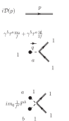
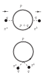
Figure 1: The Feynman rules for the Lagrangian in eq. (4) are shown on the left, where double lines denote quark propagators with Dyson-Schwinder resummation, and the blobs with attached short dashed lines stand for the non-propagating pion insertions. The one-loop Feynman diagrams for pion-pion correlators are shown in the right hand panel.

The Feynman rules for the Lagrangian in eq. (4) are shown in Figure 1, as are the Feynman diagrams for the pion two-point function. Using these rules in the diagrams we find that the causal propagator is

$$\int d^{4}x{\rm e}^{iq\cdot x}\left\langle\pi^{a}(0)\pi^{b}(x)\right\rangle=i\delta^{ab}\left[A(q^{0})^{2}-B(q^{i})^{2}-C+i\epsilon\right]^{-1},$$ (5)

where $q$ and $x$ are Minkowski 4-vectors,

$$A = -\frac{i{\cal N}}{16f^{2}}\int\frac{d^{4}p}{(2\pi)^{4}}\,{\rm Tr\/}[i{\cal D}_{11}(p)(i\gamma^{5}\gamma^{0})i{\cal D}_{11}(p+q)(i\gamma^{5}\gamma^{0})]$$

$$B = \frac{i{\cal N}(d^{4})^{2}}{16f^{2}}\int\frac{d^{4}p}{(2\pi)^{4}}\,{\rm Tr\/}[i{\cal D}_{11}(p)(i\gamma^{5}\gamma^{i})i{\cal D}_{11}(p+q)(i\gamma^{5}\gamma^{i})]$$

$$C = -\frac{i{\cal N}}{4f^{2}}\int\frac{d^{4}p}{(2\pi^{4})}\left\{m_{0}^{2}{\rm Tr\/}[i{\cal D}_{11}(p)\gamma^{5}\,i{\cal D}_{11}(p+q)\gamma_{5}]+im_{0}{\rm Tr\/}[iD_{11}(p)]\right\},$$ (6)

and the trace is over Dirac components. The flavour trace gives the factor of $\delta^{ab}$ in eq. (5), and the colour trace is subsumed into the factor of ${\cal N}$.

Since we are only interested in long-distance correlation functions of pions, we need to take the limit $q\to 0$. However, this can be done in many ways. In the chiral limit, when $m_{0}=0$, all components of $q$ go to zero together, but one can take them to zero along lines of varying $q^{0}/|\bf q|$. When $m_{0}>0$, which is physically relevant, sending $q^{0}\to 0$ while holding $|\bf q|$ fixed, gives us static correlation functions. These are the same as in the Euclidean theory Gupta:2017gbs . Here we instead take the limit where $|\bf q|\to 0$ keeping $q^{0}$ fixed, and only then take $q^{0}\to 0$. In this limit we find

$$A = \frac{{\cal N}m^{2}L}{32\pi^{2}(d^{4})^{3}f^{2}}-\frac{{\cal N}m^{2}}{2(d^{4})^{3}f^{2}}\int\frac{p^{2}dp}{(2\pi)^{2}E^{3}}n_{\scriptscriptstyle F}(E/T)$$

$$B = \frac{{\cal N}m^{2}L}{32\pi^{2}d^{4}f^{2}}+\frac{{\cal N}}{3d^{4}f^{2}}\int\frac{p^{4}dp}{(2\pi)^{2}E^{3}}n_{\scriptscriptstyle F}(E/T)$$

$$C = \frac{{\cal N}m^{2}m_{0}^{2}(1+L)}{16\pi^{2}(d^{4})^{3}f^{2}}+\frac{2{\cal N}m_{0}^{2}}{(d^{4})^{3}f^{2}}\int\frac{p^{2}dp}{(2\pi)^{2}E}n_{\scriptscriptstyle F}(E/T)$$ (7)

$$-\frac{{\cal N}m^{3}m_{0}(1+L)}{16\pi^{2}(d^{4})^{3}f^{2}}-\frac{2{\cal N}m_{0}m}{(d^{4})^{3}f^{2}}\int\frac{p^{2}dp}{(2\pi)^{2}E}n_{\scriptscriptstyle F}(E/T)$$

where $L=\log((d^{4})^{2}\mu^{2}/m^{2})$, $\mu$ is the renormalization scale of $\overline{MS}$, $n_{F}(E/T)$ is the Fermi distribution, and $E^{2}=m^{2}+p^{2}$. In general causality imposes strong restrictions on the imaginary parts of the propagator. In this case, however, since we work in the limit $q\to 0$, the imaginary parts vanish. It is useful to note that the logarithmic terms, which would survive in the limit $T\to 0$, are the same in Euclidean and real time. This non-trivial connection between real time and Euclidean propagation of pions means that the recurrent idea of inferring real time properties by measuring correlation functions of composite operators on the lattice in the Euclidean time direction using anisotropic lattices would be unproductive.

One can match the correlation function of eq. (5) with the integrals in eq. (7) to an effective pion theory with a Minkowski Lagrangian

$$L_{f}=-\frac{1}{2}c^{2}T_{0}^{2}\pi^{2}+\frac{1}{2}(\partial_{4}\pi)^{2}-\frac{1}{2}c^{4}(\nabla\pi)^{2}-\frac{c^{41}}{8}\pi^{4}.$$ (8)

which includes all terms of dimension up to 4 (the coupling $c^{41}$ requires a separate computation which we do not present here). This is valid for pion momenta $q\ll f$. Note that a kinetic term for pions is generated as usual after integrating out the quark fields. The matching involves a multiplicative renormalization of the pion field by $\sqrt{A}$, so that the kinetic term is canonically normalized. Then one has the identification $c^{4}=B/A$ and $c^{2}=C/A$. The usual definition of the pion decay constant then gives $f_{\pi}=f/\sqrt{A}$.

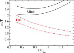
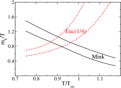
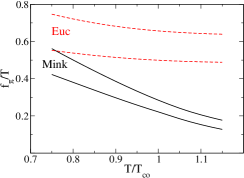
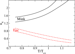
Figure 2: Comparison of various pion properties in a Euclidean theory against the corresponding property in real time, obtained using the Lagrangian in eq. (1). The couplings in the theory have been extracted from fitting to Euclidean lattice computations, and come with a band of uncertainty descended from statistical errors in the lattice measurement brandt . The upper left panel contains the rest mass $m_{r}$ (pole mass in Euclidean), the upper right has the kinetic mass $m_{k}$ (which is compared to corresponding Euclidean quantity, i.e., the screening mass divided by $u_{\pi}$; this was divided by 4 for the purpose of display), the lower left shows $f_{\pi}$, and the lower right shows $u_{\pi}$.

The dispersion relations of a slowly moving particle with dynamics obeying either eq. (1) or eq. (8) is

$$E=\sqrt{m_{r}^{2}+u^{2}p^{2}}=m_{r}+\frac{p^{2}}{2m_{k}}+\cdots$$ (9)

where the rest mass $m_{r}=d^{2}T_{0}$ and $u=d^{4}$ for a quark, and $m_{r}=\sqrt{c^{2}}T_{0}$ and $u_{\pi}=\sqrt{c^{4}}$ for a pion. The kinetic energy term contains a different mass parameter, $m_{k}=m_{r}/u^{2}$. The presence of the medium, and the consequent loss of the equivalence of different frames, forces us to distinguish between the rest mass, $m_{r}$, and the effective kinetic mass, $m_{k}$, even for particles which are moving with relativistic speeds. The Euclidean version of the rest mass $m_{r}$ has been called the pole mass. The kinetic mass $m_{k}$ has no exact analogue in the Euclidean, but may be compared with $m_{s}/u_{\pi}$, where $m_{s}$ is the screening mass. The values of both masses in real time differ from those which are measured in Euclidean lattice computations. A difference between Euclidean and real time bound state mass had been noticed earlier in the Gross-Neveu model at large $N$ precursors . This computation shows that static screening phenomena in the effective model of eq. (1) are the same in the Euclidean and Minkowski theories, whereas non-static correlators are different. As a result, the effective model of eq. (1) is a good tool for continuing the lattice computation from Euclidean into real time.

Numerical results for the temperature dependence of the parameters of the pion theory are shown in Figure 2. We note that the rest mass in real time increases roughly linearly with $T$ below the cross over temperature, $T_{co}$, and faster above that. At the lowest end of our computation we find that $m_{r}=380\pm 33$ MeV. This should be compared to the lattice input, which tunes the quark masses such that $m_{\pi}=305\pm 5$ at $T=0$. We note that this number was not an input to the fixing of the couplings in eq. (1), since we do not expect these effective theories to be valid at all temperatures. We also point out that the value of $f_{\pi}$ decreases with increasing temperature. This is consistent with the expectations of piondecay . The behaviour of $m_{k}$ is closely related to that of $u_{\pi}$. In the Euclidean computation $u_{\pi}$ falls to zero in the chiral limit at the critical point, as a result of which the pion correlations become unbounded. Even at the cross over at finite quark mass, there is a decrease in the Euclidean $u_{\pi}$. On the other hand, the real-time version shows no such decrease.

In summary, we have shown that pion propagation in Euclidean and Minkowski space time at finite temperature involves two masses: the so-called pole mass and screening mass in Euclidean, and a rest mass and kinetic mass in real time. The relationship between the two pairs is non-trivial. This is in strong contrast to the situation at $T=0$. Here we used an effective theory of self-interacting quarks, defined through eq. (1), matched to Euclidean lattice data to make the connection. The self consistency of this procedure was tested by checking that the long-wavelength limit of the static pion correlator obtained by taking $q^{0}\to 0$ before taking $|\bf q|\to 0$ agrees with the Euclidean result. We also showed that in real time $f_{\pi}$ decreases with increasing temperature, and that $u_{\pi}$ increases, in contrast to their trends on the lattice.

References

- (1) F. Karsch and H. W. Wyld, Phys. Rev. D 35, 2518 (1987).
- (2) G. Aarts and J. M. Martinez Resco, JHEP 0204, 053 (2002) [hep-ph/0203177].
- (3) P. B. Arnold, G. D. Moore and L. G. Yaffe, JHEP 0011 001 (2000) [hep-ph/0010177], JHEP 0305, 051 (2003) [hep-ph/0302165].
-
(4)
M. Asakawa, T. Hatsuda and Y. Nakahara,
Prog. Part. Nucl. Phys. 46 (2001) 459
[hep-lat/0011040];
S. Gupta, Phys. Lett. B 597 (2004) 57 doi:10.1016/j.physletb.2004.05.079 [hep-lat/0301006];
M. Kitazawa, T. Iritani, M. Asakawa and T. Hatsuda, Phys. Rev. D 96 (2017) no.11, 111502 [arXiv:1708.01415 [hep-lat]]. -
(5)
S. Sakai, A. Nakamura and T. Saito,
Nucl. Phys. A 638, 535 (1998)
[hep-lat/9810031];
F. Karsch, E. Laermann, P. Petreczky, S. Stickan and I. Wetzorke, Phys. Lett. B 530 (2002) 147 [hep-lat/0110208];
M. Asakawa and T. Hatsuda, Phys. Rev. Lett. 92 (2004) 012001 doi:10.1103/PhysRevLett.92.012001 [hep-lat/0308034];
S. Datta, F. Karsch, P. Petreczky and I. Wetzorke, Phys. Rev. D 69 (2004) 094507 [hep-lat/0312037];
H. B. Meyer, Phys. Rev. Lett. 100 (2008) 162001 [arXiv:0710.3717 [hep-lat]];
O. Philipsen and C. Schäfer, JHEP 1402 (2014) 003 doi:10.1007/JHEP02(2014)003 [arXiv:1311.6618 [hep-lat]]. -
(6)
J. Jia [ATLAS Collaboration],
J. Phys. G 38 124012 (2011)
[arXiv:1107.1468 [nucl-ex]];
G. Aad et al. [ATLAS Collaboration], JHEP 1311, 183 (2013) [arXiv:1305.2942 [hep-ex]]. - (7) S. Gupta and R. Sharma, Phys. Rev. D 97, no. 3, 036025 (2018) [arXiv:1710.05345 [hep-ph]].
- (8) S. Weinberg, “The Quantum Theory of Fields: Volume 2, Modern Applications”, Cambridge University Press, Cambridge, 1996.
- (9) Y. Nambu and G. Jona-Lasinio, Phys. Rev. 122 (1961) 345. Y. Nambu and G. Jona-Lasinio, Phys. Rev. 124 (1961) 246.
- (10) S. P. Klevansky, Rev. Mod. Phys. 64 (1992) 649.
- (11) R. L. Kobes, G. W. Semenoff and N. Weiss, Z. Phys. C 29, 371 (1985).
- (12) N. P. Landsman and C. G. van Weert, Phys. Rept. 145, 141 (1987).
- (13) B. B. Brandt, A. Francis, H. B. Meyer and D. Robaina, Phys. Rev. D 90 (2014) no.5, 054509 [arXiv:1406.5602 [hep-lat]].
- (14) S. z. Huang and M. Lissia, Phys. Rev. D 53, 7270 (1996) [hep-ph/9509360].
-
(15)
R. D. Pisarski, T. L. Trueman and M. H. G. Tytgat,
Phys. Rev. D 56, 7077 (1997)
[hep-ph/9702362];
F. Gelis, Phys. Rev. D 59, 076004 (1999) [hep-ph/9806425].