UT-19-09

DESY 19-069

Indirect Studies of Electroweakly Interacting Particles
at 100 TeV Hadron Colliders

Tomohiro Abe^(a,b), So Chigusa^(c), Yohei Ema^(d), and Takeo Moroi^(c)

^(a)Institute for Advanced Research, Nagoya University,
Furo-cho Chikusa-ku, Nagoya, Aichi, 464-8602 Japan
^(b)Kobayashi-Maskawa Institute for the Origin of Particles and the Universe,
Nagoya University, Furo-cho Chikusa-ku, Nagoya, Aichi, 464-8602 Japan
^(c)Department of Physics, Faculty of Science,
The University of Tokyo, Bunkyo-ku, Tokyo 113-0033, Japan
^(d)DESY, Notkestraße 85, D-22607 Hamburg, Germany

There are many extensions of the standard model that predict the existence of electroweakly interacting massive particles (EWIMPs), in particular in the context of the dark matter. In this paper, we provide a way for indirectly studying EWIMPs through the precise study of the pair production processes of charged leptons or that of a charged lepton and a neutrino at future $100\,\mathrm{TeV}$ collider experiments. It is revealed that this search method is suitable in particular for Higgsino, providing us the $5\sigma$ discovery reach of Higgsino in supersymmetric model with mass up to $850\,\mathrm{GeV}$. We also discuss how accurately one can extract the mass, gauge charge, and spin of EWIMPs in our method.

1 Introduction

ElectroWeakly Interacting Massive Particles (EWIMPs) are theoretically well-motivated particles that appear in many models beyond the standard model (SM). They are widely discussed in the context of the dark matter (DM), with identifying an electrically neutral (or milli-charged) component as the DM. An attractive feature of this scenario is that the vanilla thermal freeze-out scenario predicts the correct amount of the relic abundance for the EWIMP mass range of $\mathcal{O}(1\,\mathchar 45\relax\mathchar 45\relax\,10)\,\mathrm{TeV}$, and this mass range is within the scope of current and future experiments. Well-known examples of the EWIMPs are Higgsino and Wino that arise within the supersymmetric extension of the SM. Assuming that Higgsino (Wino) is the lightest supersymmetric particle and its stability is assured by the $R$-parity, its thermal relic abundance becomes consistent with the DM abundance if the mass is $1.1\,\mathrm{TeV}$ [1, 2] ($2.9\,\mathrm{TeV}$ [3, 4, 5, 2]). Another example is the minimal dark matter [6, 1, 7], where a particle with a large $SU(2)_{L}$ charge is identified as the DM. The stability is automatically assured since operators that cause its decay are suppressed by the cut-off scale of the theory thanks to the large $SU(2)_{L}$ charge, provided that one chooses a correct combination of the charge and spin. A $5$-plet Majorana fermion with a mass of $\mathcal{O}(10)\,\mathrm{TeV}$ is the most popular in this context, but there are also other possibilities, including both scalar and fermionic particles.

EWIMPs are extensively searched for by many experiments, including DM direct, indirect detections and collider searches (in particular, the mono-$X$ search and the disappearing charged track search). While EWIMPs with relatively large $SU(2)_{L}$ charges such as Wino and the 5-plet fermion are promising for these searches, Higgsino is typically more challenging to probe [8]. Given this situation, another search strategy is proposed [9, 10, 11, 12, 13, 14, 15, 16] that probes EWIMPs via the electroweak precision measurement at colliders. It utilizes a pair production of charged leptons or that of a charged lepton and a neutrino, where EWIMPs affect the pair production processes through the vacuum polarizations of the electroweak gauge bosons. It is an indirect search method in the sense that it does not produce on-shell EWIMPs as final states. The current status and future prospects have been analyzed for LHC, ILC, CLIC, and $100\,\mathrm{TeV}$ colliders [17, 18, 19], indicating that it provides a promising way to probe Higgsino as well as the other EWIMPs. A virtue of this method is that it is robust against the change of the lifetime and the decay modes of EWIMPs and whether an EWIMP constitutes a sizable portion of the DM or not. Another important point is that, due to EWIMPs, the invariant mass distributions of the final state particles show sharp dip-like behavior at the invariant mass close to twice the EWIMP mass. It helps us to distinguish the EWIMP effects from backgrounds and systematic errors.

In this paper, we pursue this indirect search method further. In particular, we demonstrate that the indirect search method can be applied not only to discover EWIMPs but also to investigate their properties, such as charges, masses, and spins. To be more specific, in this paper we focus on the future prospect of the indirect studies of EWIMPs at $100\,\mathrm{TeV}$ colliders such as FCC-$hh$ [20] and SppC [21, 22]. We update our previous analysis [14] that has considered only the neutral current (NC) processes (mediated by photon and $Z$-boson) by including the charged current (CC) processes (mediated by $W$-boson) as well, as in Refs. [15, 16]. It is crucial not only to improve the sensitivity but also to break some degeneracy among different EWIMP charge assignments; the NC and CC processes depend on different combinations of the $SU(2)_{L}$ and $U(1)_{Y}$ charges, and hence the inclusion of both processes allows us to extract these charges separately.

The rest of this paper is organized as follows. In Sec. 2, we discuss how EWIMPs affect the production processes of a charged lepton pair and those of a charged lepton and a neutrino. There we see that the EWIMP correction to the cross section, as a function of the lepton pair invariant mass, develops a dip-like structure when the invariant mass is around twice the EWIMP mass. This feature is essential in distinguishing the EWIMP effect from backgrounds and systematic errors, as discussed in detail in Sec. 3. Although we have to rely on the transverse mass instead of the invariant mass for the CC process, a similar dip-like structure appears in the transverse mass distribution. Sec. 3 is divided into three parts. First, we explain our fitting based statistical approach, in which we absorb various sources of systematic errors into a choice of nuisance parameters. Next, we study the result of the EWIMP detection reach, updating our previous results [14] by taking into account the CC processes. We then move to our main focus of this paper, namely the future prospect of the mass, charge, and spin determination of the EWIMP. Finally Sec. 4 is devoted to conclusions.

2 EWIMP effect on the lepton production processes

We investigate contributions of the EWIMPs to the Drell-Yan process through the vacuum polarization of the electroweak gauge bosons at the loop level. Throughout the paper, we assume that all the other beyond the SM particles are heavy enough so that they do not affect the following discussion. After integrating out the EWIMPs, the effective lagrangian is expressed as

$$\mathcal{L}_{\rm eff}=\mathcal{L}_{\rm SM}+C_{2}g^{2}\,W_{\mu\nu}^{a}f\left(-\frac{D^{2}}{m^{2}}\right)W^{a\mu\nu}+C_{1}g^{\prime 2}\,B_{\mu\nu}f\left(-\frac{\partial^{2}}{m^{2}}\right)B^{\mu\nu},$$ (1)

where $\mathcal{L}_{\rm SM}$ is the SM Lagrangian, $D$ is a covariant derivative, $m$ is the EWIMP mass, $g$ and $g^{\prime}$ are the $SU(2)_{L}$ and $U(1)_{Y}$ gauge coupling constants, and $W_{\mu\nu}^{a}$ and $B_{\mu\nu}$ are the field strength associated with the $SU(2)_{L}$ and $U(1)_{Y}$ gauge group, respectively. The function $f(x)$ is defined as

$$f(x)=\begin{cases}\displaystyle{\frac{1}{16\pi^{2}}\int_{0}^{1}dy\,y(1-y)\ln(1-y(1-y)x-i0)}&{\rm(Fermion)},\\[14.22636pt] \displaystyle{\frac{1}{16\pi^{2}}\int_{0}^{1}dy\,(1-2y)^{2}\ln(1-y(1-y)x-i0)}&{\rm(Scalar)},\end{cases}$$ (2)

where the first (second) line corresponds to a fermionic (scalar) EWIMP, respectively. The coefficients $C_{1}$ and $C_{2}$ for an $SU(2)_{L}$ $n$-plet EWIMP with hypercharge $Y$ are given by

$$C_{1} =\frac{\kappa}{8}nY^{2},$$ (3)

$$C_{2} =\frac{\kappa}{8}I(n),$$ (4)

where $\kappa=1,2,8,16$ for a real scalar, a complex scalar, a Weyl or Majorana fermion, and a Dirac fermion, respectively. The Dynkin index $I(n)$ for the $n$ dimensional representation of $SU(2)_{L}$ is given by

$$I(n)=\frac{1}{12}(n^{3}-n),$$ (5)

which is normalized so that $I(2)=1/2$. The coefficients are uniquely determined by the representation of the EWIMPs. For example, $(C_{1},C_{2})=(1,1)$ for Higgsino, and $(C_{1},C_{2})=(0,2)$ for Wino. We emphasize that, contrary to the usual effective field theory, our prescription is equally applied when the typical scale of the gauge boson four-momentum, $q$, is larger than the EWIMP mass scale $m$ since we do not perform a derivative expansion of $f$ in Eq. (1). It is important because, as we see soon, the effect of the EWIMPs are maximized when $\sqrt{q^{2}}\sim m$, where the derivative expansion is not applicable.

Fermion $f$	$v_{f}^{(\gamma)}$	$a_{f}^{(\gamma)}$	$v_{f}^{(Z)}$	$a_{f}^{(Z)}$	$v_{f}^{(W)}$	$a_{f}^{(W)}$
up-type quark	$\frac{2}{3}e$	0	$(\frac{1}{4}-\frac{2}{3}s_{W}^{2})g_{Z}$	$-\frac{1}{4}g_{Z}$	$\frac{1}{2\sqrt{2}}g$	$-\frac{1}{2\sqrt{2}}g$
down-type quark	$-\frac{1}{3}e$	0	$(-\frac{1}{4}+\frac{1}{3}s_{W}^{2})g_{Z}$	$\frac{1}{4}g_{Z}$	$\frac{1}{2\sqrt{2}}g$	$-\frac{1}{2\sqrt{2}}g$
lepton	$-e$	0	$(-\frac{1}{4}+s_{W}^{2})g_{Z}$	$\frac{1}{4}g_{Z}$	$\frac{1}{2\sqrt{2}}g$	$-\frac{1}{2\sqrt{2}}g$

Table 1: Coefficients of the weak interaction defined as $\Gamma_{f}^{(V)}\equiv v_{f}^{(V)}+a_{f}^{(V)}\gamma_{5}$. Here, $e=gs_{W}$ and $g_{Z}=g/c_{W}$, where $s_{W}\equiv\sin\theta_{W}$ and $c_{W}\equiv\cos\theta_{W}$ with $\theta_{W}$ being the weak mixing angle.

At the leading order (LO), we are interested in $u(p)~{}\bar{u}(p^{\prime})\to\ell^{-}(k)~{}\ell^{+}(k^{\prime})$ and $d(p)~{}\bar{d}(p^{\prime})\to\ell^{-}(k)~{}\ell^{+}(k^{\prime})$ as the NC processes and $u(p)~{}\bar{d}(p^{\prime})\to\nu(k)~{}\ell^{+}(k^{\prime})$ and $d(p)~{}\bar{u}(p^{\prime})\to\ell^{-}(k)~{}\bar{\nu}(k^{\prime})$ as the CC processes. Here, $u$ and $d$ collectively denote up-type and down-type quarks, respectively, and $p,p^{\prime},k$, and $k^{\prime}$ are initial and final state momenta. In the SM, the amplitudes for both the NC and CC processes at the LO are expressed as

$$\mathcal{M}_{\rm SM}=\sum_{V}\frac{\left[\bar{v}(p^{\prime})\gamma^{\mu}\Gamma_{q}^{(V)}u(p)\right]\left[\bar{u}(k)\gamma_{\mu}\Gamma_{\ell}^{(V)}v(k^{\prime})\right]}{s^{\prime}-m_{V}^{2}},$$ (6)

where $\sqrt{s^{\prime}}$ is the invariant mass of the final state leptons, which is denoted as $m_{\ell\ell}$ for the NC processes and $m_{\ell\nu}$ for the CC processes. The relevant gauge bosons are $V=\gamma,Z$ for the NC processes and $V=W^{\pm}$ for the CC processes, with $m_{V}$ being the corresponding gauge boson mass. In addition,

$$\Gamma_{f}^{(V)}\equiv v_{f}^{(V)}+a_{f}^{(V)}\gamma_{5},$$ (7)

with $v_{f}^{(V)}$ and $a_{f}^{(V)}$ given in Tab. 1. The EWIMP contribution is given by

$$\mathcal{M}_{\rm EWIMP}=\sum_{V,V^{\prime}}C_{VV^{\prime}}s^{\prime}f\left(\frac{s^{\prime}}{m^{2}}\right)\frac{\left[\bar{v}(p^{\prime})\gamma^{\mu}\Gamma_{q}^{(V)}u(p)\right]\left[\bar{u}(k)\gamma_{\mu}\Gamma_{\ell}^{(V^{\prime})}v(k^{\prime})\right]}{(s^{\prime}-m_{V}^{2})(s^{\prime}-m_{V^{\prime}}^{2})},$$ (8)

where $C_{\gamma\gamma}=4(C_{1}g^{\prime 2}c_{W}^{2}+C_{2}g^{2}s_{W}^{2})$, $C_{\gamma Z}=C_{Z\gamma}=4(C_{2}g^{2}-C_{1}g^{\prime 2})s_{W}c_{W}$, $C_{ZZ}=4(C_{1}g^{\prime 2}s_{W}^{2}+C_{2}g^{2}c_{W}^{2})$, and $C_{WW}=4C_{2}g^{2}$. Again $V,V^{\prime}=\gamma,Z$ for the NC processes and $V,V^{\prime}=W^{\pm}$ for the CC processes.

We use $d\Pi_{\mathrm{LIPS}}$ for a Lorentz invariant phase space factor for the two particles final state. Then, using Eqs. (6) and (8), we define

$$\frac{d\sigma_{\rm SM}}{d\sqrt{s^{\prime}}} =\sum_{a,b}\frac{dL_{ab}}{d\sqrt{s^{\prime}}}\int d\Pi_{\mathrm{LIPS}}\,\left|\mathcal{M}_{\rm SM}\left(q_{a}\bar{q}_{b}\to\ell\ell/\ell\nu\right)\right|^{2},$$ (9)

$$\frac{d\sigma_{\rm EWIMP}}{d\sqrt{s^{\prime}}} =\sum_{a,b}\frac{dL_{ab}}{d\sqrt{s^{\prime}}}\int d\Pi_{\mathrm{LIPS}}\,2\Re\left[\mathcal{M}_{\rm SM}\mathcal{M}_{\rm EWIMP}^{*}\left(q_{a}\bar{q}_{b}\to\ell\ell/\ell\nu\right)\right],$$ (10)

where we take the average and summation over spins. Here, $dL_{ab}/d\sqrt{s^{\prime}}$ is the luminosity function for a fixed $\sqrt{s^{\prime}}$:

$$\frac{dL_{ab}}{d\sqrt{s^{\prime}}}\equiv\frac{1}{s}\int_{0}^{1}dx_{1}dx_{2}~{}f_{a}(x_{1})f_{b}(x_{2})\delta\left(\frac{s^{\prime}}{s}-x_{1}x_{2}\right),$$ (11)

where $a$ and $b$ denote species of initial partons, $\sqrt{s}$ is the center of mass energy of the proton collision ($\sqrt{s}=100\,{\rm TeV}$ in our case), and $f_{a}(x)$ is a parton distribution function (PDF) of the given parton $a$. Eq. (9) represents the SM cross section, while Eq. (10) the EWIMP contribution to the cross section. For the statistical treatment in the next section, we introduce a parameter $\mu$ that parametrizes the strength of the EWMP effect, and express the cross section with $\mu$ as

$$\frac{d\tilde{\sigma}}{d\sqrt{s^{\prime}}}=\frac{d\sigma_{\rm SM}}{d\sqrt{s^{\prime}}}+\mu\frac{d\sigma_{\rm EWIMP}}{d\sqrt{s^{\prime}}}.$$ (12)

Obviously, $\mu=0$ corresponds to the pure SM, while $\mu=1$ corresponds to the SM$+$EWIMP model. Hereafter, we use

$$\delta_{\sigma}(\sqrt{s^{\prime}})\equiv\frac{d\sigma_{\rm EWIMP}/d\sqrt{s^{\prime}}}{d\sigma_{\rm SM}/d\sqrt{s^{\prime}}},$$ (13)

to denote the correction from the EWIMP.

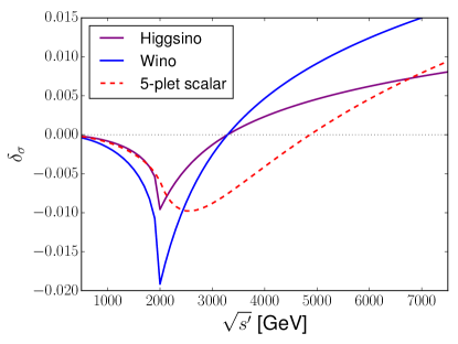
Figure 1: $\delta_{\sigma}$ for the CC processes as a function of $\sqrt{s^{\prime}}=m_{\ell\nu}$. The purple, blue, and red lines correspond to Higgsino, Wino, and 5-plet real scalar, respectively.

In Fig. 1, we plot $\delta_{\sigma}$ for the CC processes as a function of $\sqrt{s^{\prime}}$. The purple, blue, and red lines correspond to Higgsino, Wino, and 5-plet scalar, respectively. There is a dip around $\sqrt{s^{\prime}}=2m$ for all the cases of the EWIMPs which originates from the loop function $f$ in Eq. (2). The EWIMP contributions to the NC processes show a similar dip structure that again comes from $f$. This dip is crucial not only for the discovery of the EWIMP signal (see Sec. 3.3) but also for the determination of the properties of the EWIMPs (see Sec. 3.4). In particular, the EWIMP mass can be extracted from the dip position, while the EWIMP charges ($n$ and $Y$) can be determined from the depth of the dip.

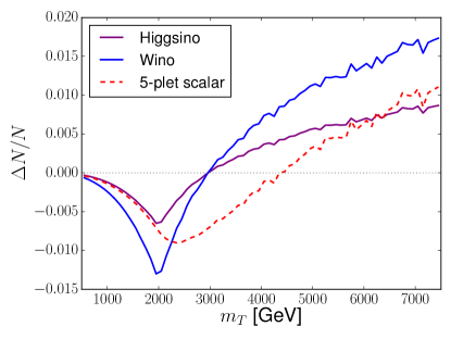
Figure 2: The EWIMP effect on the ratio of the number of events $\Delta N/N$ as a function of $m_{T}$. The line colors are the same as Fig. 1.

For the NC processes, the momenta of two final state charged leptons are measurable and we can use the invariant mass distribution of the number of events for the study of the EWIMPs. For the CC processes, on the contrary, we cannot measure the momentum of the neutrino in real experiments, and hence we instead use the missing transverse momentum $p_{T,\mathrm{miss}}$. We use the transverse mass defined as

$$m_{T}^{2}\equiv 2p_{T,\ell}\,p_{T,\mathrm{miss}}\left(1-\cos(\phi_{T,\ell,\mathrm{miss}})\right),$$ (14)

where $p_{T,\ell}$ denotes the transverse momentum of the charged lepton and $\phi_{T,\ell,\mathrm{miss}}\equiv\phi_{\ell}-\phi_{\mathrm{miss}}$ is the difference between the azimuth angles of $p_{T,\ell}$ and $p_{T,\mathrm{miss}}$. The important property of $m_{T}$ is that the distribution of $m_{T}$ peaks at $m_{T}=m_{\ell\nu}$. Because of this property, the characteristic shape of $\delta_{\sigma}$ remains in the $m_{T}$ distribution in the CC events. To see this, we plot in Fig. 2 the EWIMP effect on the number of events as a function of $m_{T}$. Here, the vertical axis is the ratio of the EWIMP correction to the number of events $\Delta N$ to the number of events in the SM $N$ for each bin with the bin width of $100\,{\rm GeV}$. We find that the dip structure remains in the $m_{T}$ distribution, though the depth of the dip is smaller compared to the $m_{\ell\nu}$ distribution.

3 Analysis

3.1 Event generation

Now we discuss how well we can extract information about EWIMPs from the invariant mass and transverse mass distributions for the processes of our concern at future $100\,\mathrm{TeV}$ $pp$ collider experiments. We take into account the effects of the next-to-leading order QCD corrections in the events as well as detector effects through Monte-Carlo simulations.

In our analysis, we first generate the SM event sets for the NC processes $pp\to e^{-}e^{+}/\mu^{-}\mu^{+}$ and for the CC processes $pp\to e^{\pm}\nu_{e}/\mu^{\pm}\nu_{\mu}$. We use MadGraph5_aMC@NLO (v2.6.3.2) [23, 24] for the event generation with the successive use of Pythia8 [25] for the parton shower and the hadronization and Delphes (v3.4.1) [26] for the detector simulation. We use NNPDF2.3QED with $\alpha_{s}(M_{Z})=0.118$ [27] as a canonical set of PDFs. For the renormalization and factorization scales, we use the default values of MadGraph5_aMC@NLO, i.e., the central $m_{T}^{2}$ scale after $k_{T}$-clustering of the event (which we denote by $Q$). The events are binned by the characteristic mass $m_{\mathrm{char}}$ for each process: we use the lepton invariant mass $m_{\mathrm{char}}=m_{\ell\ell}$ for the NC processes, and the transverse mass $m_{\mathrm{char}}=m_{T}$ for the CC processes, respectively. In both cases, we generated events with the characteristic mass within the range of $500\,\mathrm{GeV}<m_{\mathrm{char}}<7.5\,\mathrm{TeV}$ and divide them into $70$ bins with the equal width of $100\,\mathrm{GeV}$.

As for the event selection by a trigger, we may have to impose some cut on the lepton transverse momentum $p_{T}$. As we will see, we concentrate on events with high $p_{T}$ charged lepton(s) with which we expect the event may be triggered. For the NC processes, we use events with at least two high $p_{T}$ leptons. For our analysis, we use events with $m_{\ell\ell}>500\ {\rm GeV}$; we assume that such events are triggered by using two energetic charged leptons so that we do not impose extra kinematical requirements. On the contrary, the CC events are characterized only by a lepton and a missing transverse momentum. For such events, we require that the $p_{T}$ of the charged lepton should be larger than $500\,\mathrm{GeV}$. For the CC events, the cut reduces the number of events in particular for the bins with the low transverse mass $m_{T}\sim 500\,\mathrm{GeV}$, and thus affects the sensitivity of the CC processes to relatively light EWIMPs. We will come back to this point later.

The EWIMP effect is incorporated by rescaling the SM event by $\delta_{\sigma}$ defined in Eq. (13). With the parameter $\mu$ defined in Eq. (12), the number of events corresponding to the SM+EWIMP hypothesis in $i$-th bin, characterized by $m_{i,\mathrm{min}}<m_{\mathrm{char}}<m_{i,\mathrm{max}}$, is

$$x_{f,i}(\mu)=\sum_{m_{i,\mathrm{min}}<m_{\mathrm{char}}<m_{i,\mathrm{max}}}\left[1+\mu\delta_{\sigma}(\sqrt{s^{\prime}})\right],$$ (15)

where the sum runs over all the events of the final state $f$ whose characteristic mass $m_{\mathrm{char}}$ (after taking into account the detector effects) falls into the bin. Note that the true value of $\sqrt{s^{\prime}}$ should be used for each event for the computation of $\delta_{\sigma}$: we extract it from the hard process information.

3.2 Statistical treatment

We now explain the statistical method we will adopt in our analysis. We collectively denote our theoretical model as $\bm{x}_{f}(\mu)=\{x_{f,i}(\mu)\}$, where $x_{f,i}(\mu)$ is given by Eq. (15). We denote the experimental data set as $\check{\bm{x}}_{f}$ that in principle is completely unrelated to our theoretical model $\bm{x}_{f}(\mu)$. Since we do not have an actual experimental data set for $100~{}\,\mathrm{TeV}$ colliders for now, however, we take $\check{\bm{x}}_{f}=\bm{x}_{f}(\mu=1)$ (for some fixed values of the EWIMP mass and charges) throughout our analysis, assuming that the EWIMP does exist. In particular, this choice tests the SM-only hypothesis if we take our theoretical model as $\bm{x}_{f}(\mu=0)$.

If the expectation values of $x_{f,i}(\mu)$ are precisely known, the sensitivity to EWIMPs can be studied only with statistical errors. In reality, however, the computation of $x_{f,i}(\mu)$ suffers various sources of uncertainties, which results in systematic errors in our theoretical model. The sources include errors in the integrated luminosity, the beam energy, choices of the renormalization and the factorization scales, choices of PDF, the pile-up effect, higher order corrections to the cross section, and so on. In order to deal with these uncertainties, we introduce sets of free parameters $\bm{\theta}_{f}=\{\theta_{f,\alpha}\}$ (i.e. nuisance parameters) which absorb (smooth) uncertainties of the number of events, and modify our theoretical model as

$$\tilde{x}_{f,i}(\bm{\theta}_{f},\mu)\equiv x_{f,i}(\mu)f_{\mathrm{sys},i}(\bm{\theta}_{f}),$$ (16)

where $f_{\mathrm{sys},i}(\bm{\theta}_{f})$ is a function that satisfies $f_{\mathrm{sys},i}(\bm{0})=1$. We expect that, if the function $f_{\mathrm{sys},i}$ is properly chosen, the true distribution of the number of events in the SM is given by $\tilde{\bm{x}}_{f}(\bm{\theta}_{f},0)=\{\tilde{x}_{f,i}(0)f_{\mathrm{sys},i}(\bm{\theta}_{f})\}$ for some value of $\bm{\theta}_{f}$. In our analysis, we adopt the five parameters fitting function given by [30]

$$f_{\mathrm{sys},i}(\bm{\theta}_{f})=e^{\theta_{f,1}}(1+\theta_{f,2}p_{i})p_{i}^{(\theta_{f,3}+\theta_{f,4}\ln p_{i}+\theta_{f,5}\ln^{2}p_{i})},$$ (17)

where $p_{i}=2m_{i}/\sqrt{s}$ with $m_{i}$ being the central value of the lepton invariant mass (transverse mass) of the $i$-th bin for the NC (CC) processes. As we will see, the major effects of systematic errors can be absorbed into $\bm{\theta}_{f}$ with this fitting function.

In order to test the SM-only hypothesis, we define the following test statistic [31]:

$$q_{0}\equiv-2\sum_{f=\ell\ell,\ell\nu}\ln\frac{L(\check{\bm{x}}_{f};\hat{\vphantom{\rule{1.0pt}{6.14584pt}}\smash{\hat{\bm{\theta}}}}_{f},\mu=0)}{L(\check{\bm{x}}_{f};\hat{\bm{\theta}}_{f},\hat{\mu})}.$$ (18)

Here, $\hat{\vphantom{\rule{1.0pt}{6.14584pt}}\smash{\hat{\bm{\theta}}}}_{f}$ and $\{\hat{\bm{\theta}}_{f},\hat{\mu}\}$ are determined so that $\prod_{f}L(\check{\bm{x}}_{f};\bm{\theta}_{f},\mu=0)$ and $\prod_{f}L(\check{\bm{x}}_{f};\bm{\theta}_{f},\mu)$ are maximized, respectively. The likelihood function is defined as

$$L(\check{\bm{x}}_{f};\bm{\theta}_{f},\mu) \equiv L_{\bm{\theta}_{f}}(\check{\bm{x}}_{f};\mu)L^{\prime}(\bm{\theta}_{f};\bm{\sigma}_{f}),$$ (19)

where

$$L_{\bm{\theta}_{f}}(\check{\bm{x}}_{f};\mu) \equiv\prod_{i}\exp\left[-\frac{(\check{x}_{f,i}-\tilde{x}_{f,i}(\bm{\theta}_{f},\mu))^{2}}{2\tilde{x}_{f,i}(\bm{\theta}_{f},\mu)}\right],$$ (20)

$$L^{\prime}(\bm{\theta}_{f};\bm{\sigma}_{f}) \equiv\prod_{\alpha}\exp\left[-\frac{\theta_{f,\alpha}^{2}}{2\sigma_{f,\alpha}^{2}}\right].$$ (21)

The product in Eq. (20) runs over all the bins, while the product in Eq. (21) runs over all the free parameters we introduced. For each $\theta_{f,\alpha}$, we define the “standard deviation” $\sigma_{f,\alpha}$, which parametrizes the possible size of $\theta_{f,\alpha}$ within the SM with the systematic errors. If the systematic errors are negligible compared with the statistical error, we can take $\bm{\sigma}_{f}\to\bm{0}$. We identify $(q_{0})^{1/2}=5$ $(1.96)$ as the detection reach at the $5\sigma$ ($95\,\%$ C.L.) level, since $q_{0}$ asymptotically obeys a chi-square distribution with the degree of freedom one.

In order to determine $\bm{\sigma}_{f}$, we consider the following sources of the systematic errors:

• Luminosity ($\pm 5\,\%$ uncertainty is assumed),

• Renormalization scale ($2Q$ and $Q/2$, instead of $Q$),

• Factorization scale ($2Q$ and $Q/2$, instead of $Q$),

• PDF choice (We use $101$ variants of NNPDF2.3QED with $\alpha_{s}(M_{Z})=0.118$ [27] provided by LHAPDF6 [32] with IDs ranging from $244600$ to $244700$).

The values of $\bm{\sigma}_{f}$ are determined as follows. Let $\bm{y}_{f}$ be the set of number of events in the SM for the final state $f$ with the canonical choices of the parameters, and $\bm{y}^{\prime}_{f}$ be that with one of the sources of the systematic errors being varied. We minimize the chi-square function defined as

$$\chi^{2}_{f} \equiv\sum_{i}\frac{\left(y_{f,i}^{\prime}-\tilde{y}_{f,i}(\bm{\theta}_{f})\right)^{2}}{\tilde{y}_{f,i}(\bm{\theta}_{f})},$$ (22)

where

$$\tilde{y}_{f,i}(\bm{\theta}_{f}) \equiv y_{f,i}f_{\mathrm{sys},i}(\bm{\theta}_{f}),$$ (23)

for each final state $f$, and determine the best-fit values of $\bm{\theta}_{f}$ for each set of $\bm{y}^{\prime}_{f}$. We repeat this process for different sets of $\bm{y}^{\prime}_{f}$, and $\bm{\sigma}_{f}$ are determined from the distributions of the best-fit values of $\bm{\theta}_{f}$. For example, let us denote the best-fit values for the fit associated with the luminosity errors $\pm 5\%$ as $\bm{\theta}_{f}^{\pm}$. We estimate $\bm{\sigma}_{f}$ associated with these errors, denoted here as $\bm{\sigma}_{f}^{\mathrm{lumi.}}$, as

$$\sigma_{f,\alpha}^{\mathrm{lumi.}}=\sqrt{\frac{(\theta_{f,\alpha}^{+})^{2}+(\theta_{f,\alpha}^{-})^{2}}{N}},$$ (24)

where $N$ denotes the number of fitting procedures we have performed: $N=2$ for this case. We estimate $\bm{\sigma}_{f}$ associated with the other sources of the errors, denoted as $\bm{\sigma}_{f}^{\mathrm{ren.}}$, $\bm{\sigma}_{f}^{\mathrm{fac.}}$, and $\bm{\sigma}_{f}^{\mathrm{PDF}}$, in a similar manner. Finally, the total values of $\bm{\sigma}_{f}$ are obtained by combining all the sources together as

$$\sigma_{f,\alpha}=\sqrt{(\sigma_{f,\alpha}^{\mathrm{lumi.}})^{2}+(\sigma_{f,\alpha}^{\mathrm{ren.}})^{2}+(\sigma_{f,\alpha}^{\mathrm{fac.}})^{2}+(\sigma_{f,\alpha}^{\mathrm{PDF}})^{2}}.$$ (25)

Sources of systematic errors	$\sigma_{ee,1}$	$\sigma_{ee,2}$	$\sigma_{ee,3}$	$\sigma_{ee,4}$	$\sigma_{ee,5}$
Luminosity: $\pm 5\,\%$ ($\bm{\sigma}_{ee}^{\mathrm{lumi.}}$)	$0.05$	$0$	$0$	$0$	$0$
Renormalization scale: $2Q,Q/2$ ($\bm{\sigma}_{ee}^{\mathrm{ren.}}$)	$0.4$	$0.6$	$0.3$	$0.05$	$0.004$
Factorization scale: $2Q,Q/2$ ($\bm{\sigma}_{ee}^{\mathrm{fac.}}$)	$0.3$	$0.5$	$0.2$	$0.06$	$0.004$
PDF choice ($\bm{\sigma}_{ee}^{\mathrm{PDF}}$)	$0.4$	$0.7$	$0.3$	$0.06$	$0.004$

Table 2: Values of $\bm{\sigma}_{ee}$ for each source of systematic errors. The result is the same for the $\mu\mu$ final state.

Sources of systematic errors	$\sigma_{e\nu_{e},1}$	$\sigma_{e\nu_{e},2}$	$\sigma_{e\nu_{e},3}$	$\sigma_{e\nu_{e},4}$	$\sigma_{e\nu_{e},5}$
Luminosity: $\pm 5\,\%$ ($\bm{\sigma}_{e\nu_{e}}^{\mathrm{lumi.}}$)	$0.05$	$0$	$0$	$0$	$0$
Renormalization scale: $2Q,Q/2$ ($\bm{\sigma}_{e\nu_{e}}^{\mathrm{ren.}}$)	$0.3$	$0.4$	$0.2$	$0.04$	$0.003$
Factorization scale: $2Q,Q/2$ ($\bm{\sigma}_{e\nu_{e}}^{\mathrm{fac.}}$)	$1.0$	$1.6$	$0.6$	$0.1$	$0.01$
PDF choice ($\bm{\sigma}_{e\nu_{e}}^{\mathrm{PDF}}$)	$0.6$	$0.9$	$0.4$	$0.08$	$0.006$

Table 3: Best fit values of fit parameters for several sources of systematic errors for the $e\nu_{e}$ final state. The result is the same for the $\mu\nu_{\mu}$ final state.

Final state $f$	$\sigma_{f,1}$	$\sigma_{f,2}$	$\sigma_{f,3}$	$\sigma_{f,4}$	$\sigma_{f,5}$
$ee$	$0.7$	$1.0$	$0.4$	$0.09$	$0.008$
$\mu\mu$	$0.7$	$1.0$	$0.4$	$0.09$	$0.008$
$e\nu_{e}$	$1.2$	$1.9$	$0.7$	$0.2$	$0.01$
$\mu\nu_{\mu}$	$1.2$	$1.9$	$0.7$	$0.2$	$0.01$

Table 4: Summary of standard deviations $\bm{\sigma}_{f}$ for each final state.

In Table 2 and 3, we show the values of $\bm{\sigma}_{ee}$ and $\bm{\sigma}_{e\nu_{e}}$ associated with each source of the systematic errors, respectively. These values can be interpreted as the possible size of the fit parameters within the SM, which is caused by the systematic uncertainties. As explained in Eq. (25), we combine these values in each column to obtain $\bm{\sigma}_{f}$. In Table 4, we summarize the result of the combination for all the final states. The values of $\bm{\sigma}_{f}$ are independent of the final state lepton flavors since the energy scale of our concern is much higher than the lepton masses. However, we use different sets of fit parameters $\bm{\theta}_{ee}$ and $\bm{\theta}_{\mu\mu}$ for the NC processes and $\bm{\theta}_{e\nu_{e}}$ and $\bm{\theta}_{\mu\nu_{\mu}}$ for the CC processes because of the different detector response to electrons and muons.

3.3 Detection reach

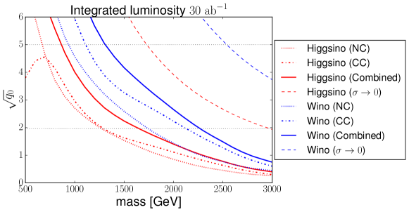
Figure 3: $\sqrt{q_{0}}$ as a function of the EWIMP mass. Red and blue lines correspond to the Higgsino and the Wino, respectively, while line styles represent the result from the NC processes, the CC processes, the combined analysis, and the combined analysis with the optimistic $\bm{\sigma}_{f}\to\bm{0}$ limit.

Now we show the detection reach of EWIMPs at future $100\,\mathrm{TeV}$ colliders. In Fig. 3, we plot the value of $\sqrt{q_{0}}$ as a function of the EWIMP mass, with the integrated luminosity $\mathcal{L}=30\,\mathrm{ab}^{-1}$. As representative scenarios, we show the cases for Higgsino (the red lines) and Wino (the blue lines). The dotted and dash-dotted lines are the result obtained only from the NC processes and the CC processes, respectively. We find that the CC processes are more sensitive to the effect of the EWIMPs than the NC processes because of the larger cross section. This result is consistent with Refs. [15, 16]. The sensitivity of the CC processes is weakened for $m\lesssim 700\,\mathrm{GeV}$ because of the lepton $p_{T}$ cut we have applied. The combined results of the NC and CC processes are shown by the solid lines. By combining the two types of processes, the $5\sigma$ discovery reaches ($95\,\%$ C.L. bounds) for Higgsino and Wino are $850\,\mathrm{GeV}$ ($1.7\,\mathrm{TeV}$) and $1.3\,\mathrm{TeV}$ ($2.3\,\mathrm{TeV}$), respectively. We find that the combination of the NC and CC processes improves the sensitivity of the EWIMP mass. Furthermore, if we understand all the systematic uncertainties quite well and effectively take the $\bm{\sigma}_{f}\to\bm{0}$ limit in the combined result, the detection reach will be pushed up significantly as shown by the dashed lines: $1.1\,\mathrm{TeV}$ Higgsino signal at well above $5\sigma$ level and a $4\sigma$ hint of the $2.9\,\mathrm{TeV}$ Wino. Therefore, it is essential to reduce the systematic uncertainties for the detection of EWIMPs through the NC and CC processes.

3.4 Determination of EWIMP properties

In this subsection, we show that it is possible to determine the properties of the EWIMPs from the NC and CC processes, thanks to the fact that we can study the $m_{\ell\ell}$ and $m_{T}$ distribution in great detail for these processes. Some information about the mass, charge, and spin of the EWIMPs can be extracted because the corrections to these distributions from the EWIMPs are completely determined by these EWIMP properties. Firstly, we can extract the EWIMP mass from the position of the dip-like structure in the correction since it corresponds to roughly twice the EWIMP mass as we have shown in Sec. 2. Secondly, the overall size of the correction gives us information about the $SU(2)_{L}$ and $U(1)_{Y}$ charges. The CC processes depend only on the $SU(2)_{L}$ charge, while the NC processes depend both on the $SU(2)_{L}$ and $U(1)_{Y}$ charges. Consequently, we can obtain information about the gauge charges of the EWIMPs from the NC and CC processes.

We now demonstrate the mass and charge determination of fermionic EWIMPs. This is equivalent to the determination of the parameter set $(m,C_{1},C_{2})$. We generate the data assuming the SM $+$ EWIMP model ($\mu=1$) with some specific values of $m,n,Y$, and $\kappa$, with which we obtain $(m,C_{1},C_{2})$. We fix $\mu=1$ for our theoretical model as well, and hence the theoretical predictions of the number of events also depend on these three parameters, $\bm{x}_{f}=\bm{x}_{f}(m,C_{1},C_{2})$. We define the likelihood function $L(\check{\bm{x}}_{f};\bm{\theta}_{f},m,C_{1},C_{2})$ in the same form as Eqs. (16) and (19) with the theoretical prediction $\bm{x}_{f}$ now understood as a function of $(m,C_{1},C_{2})$, not of $\mu$. The test statistic is defined as

$$q(m,C_{1},C_{2})\equiv-2\sum_{f}\ln\frac{L(\check{\bm{x}}_{f};\hat{\vphantom{\rule{1.0pt}{6.14584pt}}\smash{\hat{\bm{\theta}}}}_{f},m,C_{1},C_{2})}{L(\check{\bm{x}}_{f};\hat{\bm{\theta}}_{f},\hat{m},\hat{C}_{1},\hat{C}_{2})},$$ (26)

where the parameters $(\{\hat{\bm{\theta}}_{f}\},\hat{m},\hat{C}_{1},\hat{C}_{2})$ maximize $\prod_{f}L(\check{\bm{x}}_{f};\bm{\theta}_{f},m,C_{1},C_{2})$, while $\hat{\vphantom{\rule{1.0pt}{6.14584pt}}\smash{\hat{\bm{\theta}}}}_{f}$ maximize $L(\check{\bm{x}}_{f};\bm{\theta}_{f},{m},{C}_{1},C_{2})$ for fixed values of $(m,C_{1},C_{2})$. It follows the chi-squared distribution with three degrees of freedom in the limit of a large number of events [33]. The test statistic defined in this way examines the compatibility of a given EWIMP model (i.e. a parameter set $(m,C_{1},C_{2})$) with the observed signal.

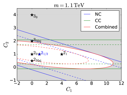
Figure 4: Contour of $\sqrt{q}$ in the $C_{1}~{}\mathrm{vs.}~{}C_{2}$ plane with $m=1.1\,\mathrm{TeV}$, where we assume $1.1\,\mathrm{TeV}$ Higgsino signal. The dotted and solid lines denote $1\sigma$ and $2\sigma$ contours, respectively, and the gray region corresponds to the parameter space that is in tension with the observation at more than $2\sigma$ level. The blue, green, and red lines correspond to the result from the NC processes, the CC processes, and the combined analysis, respectively. Each star marker annotated as “$n_{Y}$” represents a point corresponding to a $SU(2)_{L}$ $n$-plet Dirac fermion with hypercharge $Y$, while that with “$n_{\mathrm{Maj}}$” corresponds to an $SU(2)_{L}$ $n$-plet Majorana fermion.

Once a deviation from the SM prediction is observed in a real experiment, we may determine $(m,C_{1},C_{2})$ using the above test statistic $q$. In the following, we show the expected accuracy of the determination of $(m,C_{1},C_{2})$ for the case where there exists $1.1\,\mathrm{TeV}$ Higgsino.

In Fig. 4, we show the contours of $1\sigma$ (dotted) and $2\sigma$ (solid) constraints, which correspond to the values $\sqrt{q}=1.9$ and $\sqrt{q}=2.8$, respectively, in the $C_{1}~{}\mathrm{vs.}~{}C_{2}$ plane for $m=1.1\,\mathrm{TeV}$. The blue, green, and red lines denote the result obtained from the NC processes, the CC processes, and the combined analysis, respectively. The models in the gray region are in more than $2\sigma$ tension with the observation. We also show several star markers that correspond to the single $SU(2)_{L}$ multiplet contributions: the markers with “$n_{Y}$” represent an $SU(2)_{L}$ $n$-plet Dirac fermion with hypercharge $Y$, while those with “$n_{\mathrm{Maj}}$” an $SU(2)_{L}$ $n$-plet Majorana fermion. Both the NC and CC constraints are represented as straight bands in the $C_{1}~{}\mathrm{vs.}~{}C_{2}$ plane since each process depends on a specific linear combination of $C_{1}$ and $C_{2}$. In particular, the CC constraint is independent of $C_{1}$, or $Y$. In this sense, the NC and CC processes are complementary to each other, and thus we can separately constrain $C_{1}$ and $C_{2}$ only after combining these two results. For instance, we can exclude a single fermionic $SU(2)_{L}$ multiplet with $n\neq 2$ at more than $2\sigma$ level, although each process by itself cannot exclude the possibility of $3_{\text{Maj}}$. We can also constrain the hypercharge, yet it is not uniquely determined. In addition to the Higgsino, the EWIMP as an $SU(2)_{L}$ doublet Dirac fermion with $|Y|^{2}\lesssim 2$ or an $SU(2)_{L}$ doublet Majorana fermion with $|Y|^{2}\lesssim 5$ is still allowed.

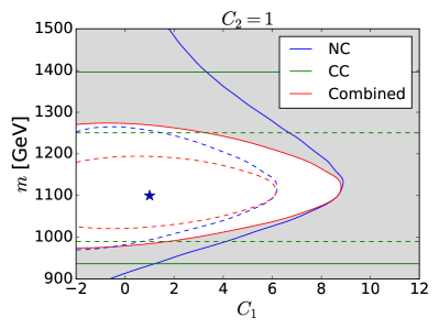
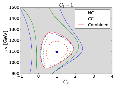
Figure 5: Left: Contour of $\sqrt{q}$ in the $C_{1}~{}\mathrm{vs.}~{}m$ plane with $C_{2}=1$, where we assume the $1.1\,\mathrm{TeV}$ Higgsino signal. The colors and styles of lines and the meaning of the gray region are the same as Fig. 4. The star maker corresponds to the true Higgsino property $(C_{1},m)=(1,1.1\,\mathrm{TeV})$. Right: Contour of $\sqrt{q}$ in the $C_{2}~{}\mathrm{vs.}~{}m$ plane for $C_{1}=1$, where we assume the $1.1\,\mathrm{TeV}$ Higgsino signal. The star maker corresponds to the true Higgsino property $(C_{2},m)=(1,1.1\,\mathrm{TeV})$.

In Fig. 5, we show the contour plots of $\sqrt{q}$ in the $C_{1}~{}\mathrm{vs.}~{}m$ plane with $C_{2}=1$ (left) and those in the $C_{2}~{}\mathrm{vs.}~{}m$ plane with $C_{1}=1$ (right). The star marker in each panel shows the true values of parameters $(C_{1},m)=(1,1.1\,\mathrm{TeV})$ (left) and $(C_{2},m)=(1,1.1\,\mathrm{TeV})$ (right). Again, by combining the NC and CC results, we can significantly improve the determination of EWIMP properties, making $1\sigma$ and $2\sigma$ contours closed circles in the planes of our concern. In particular, as red lines show, the combined analysis allows us to determine the observed EWIMP mass at the level of $\mathcal{O}(10)\%$.

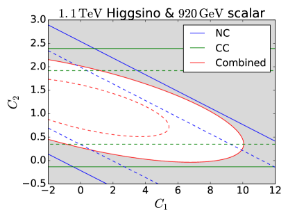
Figure 6: Contour of $\sqrt{q}$ in the $C_{1}~{}\mathrm{vs.}~{}C_{2}$ plane for the $1.1\,\mathrm{TeV}$ Higgsino signal, tested with the scalar EWIMP assumption. The plane is defined as the scalar mass of $920\,\mathrm{GeV}$. The colors and styles of lines and the meaning of the gray region are the same as Fig. 4.

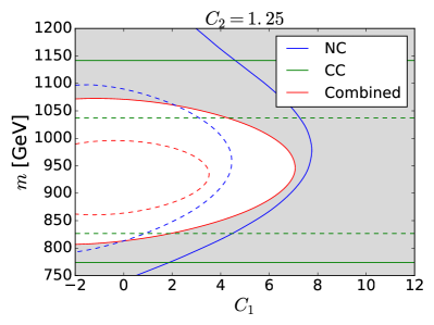
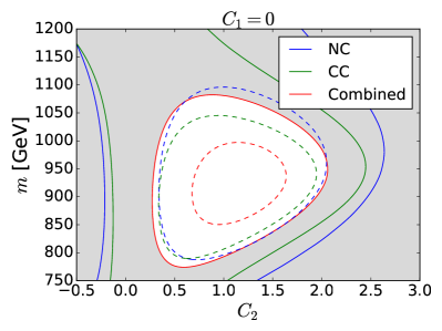
Figure 7: Left: Contour of $\sqrt{q}$ in the $C_{1}~{}\mathrm{vs.}~{}m$ plane with $C_{2}=1.25$ for the $1.1\,\mathrm{TeV}$ Higgsino signal, tested with the scalar EWIMP assumption. The colors and styles of lines and the meaning of the gray region are the same as Fig. 4. Right: Contour of $\sqrt{q}$ in the $C_{2}~{}\mathrm{vs.}~{}m$ plane with $C_{1}=0$ for the $1.1\,\mathrm{TeV}$ Higgsino signal, tested with the scalar EWIMP assumption.

Finally, we comment on the possibility of discriminating between fermionic and scalar EWIMPs, whose difference comes from the loop function $f(x)$ (see Eq. (2)). Here we repeat the same analysis explained above, assuming the $1.1\,\mathrm{TeV}$ Higgsino signal for example, but use the scalar loop function to evaluate the theoretical predictions $\bm{x}_{f}(m,C_{1},C_{2})$. In Figs. 6 and 7, we show the results in the $C_{1}$ vs. $C_{2}$ plane and the $C_{1}$ (or $C_{2}$) vs. $m$ plane, respectively, where one of the three parameters is fixed to its best fit value. It is seen that, in the case of the $1.1\,\mathrm{TeV}$ Higgsino signal, it is hard to distinguish between the bosonic and fermionic EWIMPs only with our method. However, if a part of the EWIMP properties (in particular its mass) is determined from another approach, our method may allow us to determine its spin correctly.

We also stress here that, with some favorable assumption about the observed signal, we may obtain some hint about its spin. For example, if we assume that the observed signal composes a fraction of the dark matter in our Universe, the choice of the EWIMP charges is significantly constrained. Note from Fig. 6 that the only choices of EWIMP charges that allow the EWIMP multiplet to contain an electrically neutral component are $(n,|Y|)=(3,0),(3,1),(4,1/2),(4,3/2)$, and $(5,0)_{\text{real}}$. The last column of the table 5 shows proper choices of EWIMP masses in order for their thermal relic abundances become comparable with the dark matter abundance in the current Universe. All of those values are somewhat larger than the central value of the mass of the observed signal, which means that the scalar interpretation of the signal cannot explain the whole of the dark matter relic abundance without introducing some non-thermal production mechanism.

$(n,Y)$	$C_{1}$	$C_{2}$	$m_{\text{DM}}$[TeV]
$(3,0)_{\text{real}}$	0	0.25	2.5 [34]
$(3,0)$	0	0.5	1.55 [35]
$(3,1)$	0.75	0.5	1.6 [34]
$(4,\frac{1}{2})$	0.25	1.25	2.4 [34]
$(4,\frac{3}{2})$	2.25	1.25	2.9 [34]
$(5,0)_{\text{real}}$	0	1.25	9.4 [34]

Table 5: The scalar EWIMPs that are compatible with the result in Fig. 6. The observed DM energy density is explained by the thermal relic of the EWIMP with $m_{\text{DM}}$ shown in the fourth column.

4 Conclusion

In this paper, we have discussed the indirect search of EWIMPs at future $100\,\mathrm{TeV}$ hadron colliders based on the precision measurement of the production processes of a charged lepton pair and that of a charged lepton and a neutrino. In particular, we have demonstrated that not only we can discover the EWIMPs, but also we can determine their properties such as their masses, $SU(2)_{L}$ and $U(1)_{Y}$ charges, and spins via the processes of our concern. It is based on two facts: the high energy lepton production channel enables us to study its momentum distribution in great detail, and the EWIMP correction shows characteristic features, including a dip-like structure as the final state invariant mass being twice the EWIMP mass. The latter feature also helps us to distinguish the EWIMP signals from backgrounds and systematic errors, as they are not expected to show a dip-like structure. In order to fully exploit the differences between the distributions the EWIMP signals and systematic errors, we have adopted the fitting based analysis as our statistical treatment.

First, we have shown in Fig. 3 the detection reach of Higgsino and Wino from the neutral current (NC) processes (mediated by photon or $Z$-boson), the charged current (CC) processes (mediated by $W$-boson), and the combination of these two results. We have seen that the addition of the CC processes improves the detection reach from the previous analysis [14]. From the combined analysis, the bounds at the $5\sigma$ ($95\%$ C.L.) level for Higgsino and Wino are $850\,\mathrm{GeV}$ ($1.7\,\mathrm{TeV}$) and $1.3\,\mathrm{TeV}$ ($2.3\,\mathrm{TeV}$), respectively. This result, in particular that for short lifetime Higgsino, indicates the importance of our method for the EWIMP search.

Next, we have considered the determination of the mass and $SU(2)_{L}$ and $U(1)_{Y}$ charges of the observed EWIMP. By combining the NC and the CC events, the position and the height of the dip in the EWIMP effect on the cross section gives us enough information for determining all the three parameters. In Figs. 4 and 5, we have shown the plots of the test statistics that test the validity of several choices of parameters. As a result, the $SU(2)_{L}$ charge of the observed signal is correctly identified under the assumption of a single EWIMP multiplet, and the $U(1)_{Y}$ charge and mass are also determined precisely. In order for the determination of the EWIMP spin, we have plotted the contours of the test statistics that test the validity of the scalar EWIMP models with some fixed values of masses and charges. The results are shown in Figs. 6 and 7, which reveals that the spin is not completely determined by solely using our method. Use of another approach to determine the EWIMP properties, or of some assumption like that the observed signal corresponds to the dark matter in our Universe, may help us to obtain further information regarding the EWIMP spin.

References

- [1] M. Cirelli, A. Strumia, M. Tamburini, Cosmology and Astrophysics of Minimal Dark Matter, Nucl. Phys. B787 (2007) 152–175. arXiv:0706.4071, doi:10.1016/j.nuclphysb.2007.07.023.
- [2] N. Arkani-Hamed, A. Delgado, G. F. Giudice, The Well-tempered neutralino, Nucl. Phys. B741 (2006) 108–130. arXiv:hep-ph/0601041, doi:10.1016/j.nuclphysb.2006.02.010.
- [3] J. Hisano, S. Matsumoto, M. Nagai, O. Saito, M. Senami, Non-perturbative effect on thermal relic abundance of dark matter, Phys. Lett. B646 (2007) 34–38. arXiv:hep-ph/0610249, doi:10.1016/j.physletb.2007.01.012.
- [4] T. Moroi, M. Nagai, M. Takimoto, Non-Thermal Production of Wino Dark Matter via the Decay of Long-Lived Particles, JHEP 07 (2013) 066. arXiv:1303.0948, doi:10.1007/JHEP07(2013)066.
- [5] M. Beneke, A. Bharucha, F. Dighera, C. Hellmann, A. Hryczuk, S. Recksiegel, P. Ruiz-Femenia, Relic density of wino-like dark matter in the MSSM, JHEP 03 (2016) 119. arXiv:1601.04718, doi:10.1007/JHEP03(2016)119.
- [6] M. Cirelli, N. Fornengo, A. Strumia, Minimal dark matter, Nucl. Phys. B753 (2006) 178–194. arXiv:hep-ph/0512090, doi:10.1016/j.nuclphysb.2006.07.012.
- [7] M. Cirelli, A. Strumia, Minimal Dark Matter: Model and results, New J. Phys. 11 (2009) 105005. arXiv:0903.3381, doi:10.1088/1367-2630/11/10/105005.
- [8] H. Baer, A. Mustafayev, X. Tata, Monojets and mono-photons from light higgsino pair production at LHC14, Phys. Rev. D89 (5) (2014) 055007. arXiv:1401.1162, doi:10.1103/PhysRevD.89.055007.
- [9] D. S. M. Alves, J. Galloway, J. T. Ruderman, J. R. Walsh, Running Electroweak Couplings as a Probe of New Physics, JHEP 02 (2015) 007. arXiv:1410.6810, doi:10.1007/JHEP02(2015)007.
- [10] C. Gross, O. Lebedev, J. M. No, Drell-Yan constraints on new electroweak states: LHC as a precision machine, Mod. Phys. Lett. A32 (16) (2017) 1750094. arXiv:1602.03877, doi:10.1142/S0217732317500948.
- [11] M. Farina, G. Panico, D. Pappadopulo, J. T. Ruderman, R. Torre, A. Wulzer, Energy helps accuracy: electroweak precision tests at hadron colliders, Phys. Lett. B772 (2017) 210–215. arXiv:1609.08157, doi:10.1016/j.physletb.2017.06.043.
- [12] K. Harigaya, K. Ichikawa, A. Kundu, S. Matsumoto, S. Shirai, Indirect Probe of Electroweak-Interacting Particles at Future Lepton Colliders, JHEP 09 (2015) 105. arXiv:1504.03402, doi:10.1007/JHEP09(2015)105.
- [13] S. Matsumoto, S. Shirai, M. Takeuchi, Indirect Probe of Electroweakly Interacting Particles at the High-Luminosity Large Hadron Collider, JHEP 06 (2018) 049. arXiv:1711.05449, doi:10.1007/JHEP06(2018)049.
- [14] S. Chigusa, Y. Ema, T. Moroi, Probing electroweakly interacting massive particles with Drell-Yan process at 100 TeV hadron colliders, Phys. Lett. B789 (2019) 106–113. arXiv:1810.07349, doi:10.1016/j.physletb.2018.12.011.
- [15] L. Di Luzio, R. Gröber, G. Panico, Probing new electroweak states via precision measurements at the LHC and future colliders, JHEP 01 (2019) 011. arXiv:1810.10993, doi:10.1007/JHEP01(2019)011.
- [16] S. Matsumoto, S. Shirai, M. Takeuchi, Indirect Probe of Electroweak-Interacting Particles with Mono-Lepton Signatures at Hadron CollidersarXiv:1810.12234.
- [17] M. L. Mangano, et al., Physics at a 100 TeV pp Collider: Standard Model Processes, CERN Yellow Report (3) (2017) 1–254. arXiv:1607.01831, doi:10.23731/CYRM-2017-003.1.
- [18] R. Contino, et al., Physics at a 100 TeV pp collider: Higgs and EW symmetry breaking studies, CERN Yellow Report (3) (2017) 255–440. arXiv:1606.09408, doi:10.23731/CYRM-2017-003.255.
- [19] T. Golling, et al., Physics at a 100 TeV pp collider: beyond the Standard Model phenomena, CERN Yellow Report (3) (2017) 441–634. arXiv:1606.00947, doi:10.23731/CYRM-2017-003.441.
-
[20]
M. Benedikt, M. Capeans Garrido, F. Cerutti, B. Goddard, J. Gutleber, J. M.
Jimenez, M. Mangano, V. Mertens, J. A. Osborne, T. Otto, J. Poole,
W. Riegler, D. Schulte, L. J. Tavian, D. Tommasini, F. Zimmermann,
Future Circular Collider, Tech.
Rep. CERN-ACC-2018-0058, CERN, Geneva, submitted for publication to Eur.
Phys. J. ST. (Dec 2018).
URL https://cds.cern.ch/record/2651300 - [21] CEPC-SPPC Study Group, CEPC-SPPC Preliminary Conceptual Design Report. 1. Physics and Detector, CEPC-SPPC Preliminary Conceptual Design Report. 1. Physics and Detector.
- [22] CEPC-SPPC Study Group, CEPC-SPPC Preliminary Conceptual Design Report. 2. Accelerator, CEPC-SPPC Preliminary Conceptual Design Report. 2. Accelerator.
- [23] J. Alwall, M. Herquet, F. Maltoni, O. Mattelaer, T. Stelzer, MadGraph 5 : Going Beyond, JHEP 06 (2011) 128. arXiv:1106.0522, doi:10.1007/JHEP06(2011)128.
- [24] J. Alwall, R. Frederix, S. Frixione, V. Hirschi, F. Maltoni, O. Mattelaer, H. S. Shao, T. Stelzer, P. Torrielli, M. Zaro, The automated computation of tree-level and next-to-leading order differential cross sections, and their matching to parton shower simulations, JHEP 07 (2014) 079. arXiv:1405.0301, doi:10.1007/JHEP07(2014)079.
- [25] T. Sjöstrand, S. Ask, J. R. Christiansen, R. Corke, N. Desai, P. Ilten, S. Mrenna, S. Prestel, C. O. Rasmussen, P. Z. Skands, An Introduction to PYTHIA 8.2, Comput. Phys. Commun. 191 (2015) 159–177. arXiv:1410.3012, doi:10.1016/j.cpc.2015.01.024.
- [26] J. de Favereau, C. Delaere, P. Demin, A. Giammanco, V. Lemaître, A. Mertens, M. Selvaggi, DELPHES 3, A modular framework for fast simulation of a generic collider experiment, JHEP 02 (2014) 057. arXiv:1307.6346, doi:10.1007/JHEP02(2014)057.
- [27] R. D. Ball, V. Bertone, S. Carrazza, L. Del Debbio, S. Forte, A. Guffanti, N. P. Hartland, J. Rojo, Parton distributions with QED corrections, Nucl. Phys. B877 (2013) 290–320. arXiv:1308.0598, doi:10.1016/j.nuclphysb.2013.10.010.
- [28] M. Aaboud, et al., Search for a new heavy gauge boson resonance decaying into a lepton and missing transverse momentum in 36 fb-1 of collisions at 13 TeV with the ATLAS experiment, Eur. Phys. J. C78 (5) (2018) 401. arXiv:1706.04786, doi:10.1140/epjc/s10052-018-5877-y.
- [29] A. M. Sirunyan, et al., Search for high-mass resonances in final states with a lepton and missing transverse momentum at TeV, JHEP 06 (2018) 128. arXiv:1803.11133, doi:10.1007/JHEP06(2018)128.
- [30] T. Aaltonen, et al., Search for new particles decaying into dijets in proton-antiproton collisions at s**(1/2) = 1.96-TeV, Phys. Rev. D79 (2009) 112002. arXiv:0812.4036, doi:10.1103/PhysRevD.79.112002.
- [31] G. Cowan, K. Cranmer, E. Gross, O. Vitells, Asymptotic formulae for likelihood-based tests of new physics, Eur. Phys. J. C71 (2011) 1554, [Erratum: Eur. Phys. J.C73,2501(2013)]. arXiv:1007.1727, doi:10.1140/epjc/s10052-011-1554-0,10.1140/epjc/s10052-013-2501-z.
- [32] A. Buckley, J. Ferrando, S. Lloyd, K. Nordström, B. Page, M. Rüfenacht, M. Schönherr, G. Watt, LHAPDF6: parton density access in the LHC precision era, Eur. Phys. J. C75 (2015) 132. arXiv:1412.7420, doi:10.1140/epjc/s10052-015-3318-8.
- [33] M. Tanabashi, et al., Review of Particle Physics, Phys. Rev. D98 (3) (2018) 030001. doi:10.1103/PhysRevD.98.030001.
- [34] M. Farina, D. Pappadopulo, A. Strumia, A modified naturalness principle and its experimental tests, JHEP 08 (2013) 022. arXiv:1303.7244, doi:10.1007/JHEP08(2013)022.
- [35] E. Del Nobile, M. Nardecchia, P. Panci, Millicharge or Decay: A Critical Take on Minimal Dark Matter, JCAP 1604 (04) (2016) 048. arXiv:1512.05353, doi:10.1088/1475-7516/2016/04/048.