Efficient parallel algorithm for estimating higher-order polyspectra

Joseph Tomlinson Department of Astronomy and Astrophysics and Institute for Gravitation and the Cosmos,
The Pennsylvania State University, University Park, PA 16802, USA
Donghui Jeong Department of Astronomy and Astrophysics and Institute for Gravitation and the Cosmos,
The Pennsylvania State University, University Park, PA 16802, USA
Juhan Kim Center for Advance Computation, Korea Institute for Advanced Study, 85 Hoegiro, Dongdaemun-gu, Seoul 130-722, Korea
(Received XXX; Revised YYY; Accepted ZZZ)
Abstract

Nonlinearities in the gravitational evolution, galaxy bias, and redshift-space distortion drive the observed galaxy density fields away from the initial near-Gaussian states. Exploiting such a non-Gaussian galaxy density field requires measuring higher-order correlation functions, or, its Fourier counterpart, polyspectra. Here, we present an efficient parallel algorithm for estimating higher-order polyspectra. Based upon the Scoccimarro estimator, the estimator avoids direct sampling of polygons by using the Fast-Fourier Transform (FFT), and the parallelization overcomes the large memory requirement of the original estimator. In particular, we design the memory layout to minimize the inter-CPU communications, which excels in the code performance.

cosmology: large-scale structure of universe — methods: data analysis
journal: ApJ

1 Introduction

The primordial density field in the Universe measured by the temperature anisotropies and polarizations of cosmic microwave background (CMB) radiation is very close to Gaussian (Planck Collaboration, 2016). In contrast, the observed galaxy density field shows strong non-Gaussianity due to late-time effects such as nonlinear gravitational instability, nonlinear galaxy bias as well as nonlinear redshift-space distortion.

The analysis of the galaxy density field in literature is yet focusing on the galaxy two-point correlation function, or its Fourier counterpart, the galaxy power spectrum (Tegmark et al., 2006; Blake et al., 2011; Parkinson et al., 2012; Reid et al., 2012; de la Torre et al., 2013; Pezzotta et al., 2017)). At the same time, the interest in the higher-order correlation functions and polyspectra has emerged to complement the two-point statistics in exploiting such a non-Gaussian galaxy density field. In Fourier space, these are, from third order, bispectrum, trispectrum, quadspectrum, pentaspectrum, hexaspectrum, and so on.

Thus far, the analysis on the higher-order correlation functions and polyspectra focuses mainly on the galaxy bispectrum and three-point correlation function (Scoccimarro et al., 2001; Verde et al., 2002; Gaztañaga et al., 2005; Nichol et al., 2006; Nishimichi et al., 2007; Marín, 2011; McBride et al., 2011b, a; Gil-Marín et al., 2015; Marín et al., 2013), but they have not been as informative as their lower-order counterparts. This is due to both the high computational cost in estimating higher-order correlation functions and the lack of accurate modeling needed for detailed data analysis.

One challenge in studying the higher-order polyspectrum in Fourier space is to find an efficient estimator; when estimating n𝑛n-th order polyspectrum, the complexity of the naive estimator grows as the number of all possible n𝑛n-gons in the three-dimensional Fourier space that scales as Nmax3(n1)superscriptsubscript𝑁max3𝑛1N_{\rm max}^{3(n-1)}. Here, Nmaxkmax/δksubscript𝑁maxsubscript𝑘max𝛿𝑘N_{\rm max}\equiv k_{\rm max}/\delta k is the number of one-dimensional discrete grid points of interest, with kmaxsubscript𝑘maxk_{\rm max} being the maximum wavenumber of the analysis, usually set by the smallest scale that we can reliably model the nonlinearities in galaxy density field, and δk𝛿𝑘\delta k being the size of the binning in Fourier space.

One can alleviate this computational cost by using the Fourier space representation of the Dirac-delta operator that dictates the statistical homogeneity. Originally done by Scoccimarro (2000) for estimating the bispectrum, in this way, we can estimate a polyspectrum by taking advantage of the Fast Fourier transformation algorithm. As we shall outline in Sec. 2, the calculation of the polyspectrum then boils down to a sum of products of the Nmaxsubscript𝑁maxN_{\rm max} distinct three-dimensional Fourier volumes derived from the original density field. This method avoids directly sampling all n𝑛n-gons and is computationally much faster for all high-order polyspectra.

The implementation of the Fourier based method, however, requires allocating a large amount of memory. To avoid the aliasing problem associated with the Fourier method, the three-dimensional Fourier grid must be at least (sNmax)3superscript𝑠subscript𝑁max3(sN_{\rm max})^{3} for the s𝑠s-point polyspectrum; as we need a total of Nmaxsubscript𝑁maxN_{\rm max} such three-dimensional Fourier volumes, the memory requirement grows as s3Nmax4superscript𝑠3superscriptsubscript𝑁max4s^{3}N_{\rm max}^{4}. For example, the memory requirement to estimate the bispectrum (s=3𝑠3s=3) with Nmax=128subscript𝑁max128N_{\rm max}=128, when using single precision, is already 27 Gigabytes.

In this paper, we shall improve the performance of the polyspectra estimators by parallelizing them. The most straightforward and naive approach might be to distribute each of the Fourier volumes to a different processor. To compute the polyspectum, then we need to calculate the sum of the multiplication of the Fourier volumes in different processors. This proves to be quite slow and, if not slower, only marginally faster than even the direct calculation from sampling all possible n𝑛n-polygons. Instead, we distribute the Fourier volumes to parallel nodes so that the summation can be done almost entirely locally. Here, most of the inter-processor communication occurs during the Fourier transform step and the performance is significantly faster than the serial estimator. In this paper, we shall demonstrate the performance of this parallel algorithm for efficient calculation of higher-order polyspectra.

This paper is organized as follows. In Sec. 2 we discuss the Scoccimarro estimator and its extension to higher-order polyspectra and the limitations of such an extension. In Sec. 3 we explain our efficient method of parallelization for this estimator. Sec. 4 analyzes the results of our application of the estimator to a grid of unity, equivalent to calculating the number of polygons, for a variety of high-order polyspectra and also includes an analysis of the scaling of our parallel algorithm. We conclude in Sec. 5. App. A discusses the conversion of our general estimator from integral to summation form for direct application to calculations. Finally, App. B discusses some approximately analytic solutions to the number of n𝑛n-gons in three-dimensional Fourier space.

We use the following convention

δ(𝒌)=𝛿𝒌absent\displaystyle\delta({\bm{k}})= d3xδ(𝒙)ei𝒌𝒙,superscript𝑑3𝑥𝛿𝒙superscript𝑒𝑖𝒌𝒙\displaystyle\int d^{3}x\delta(\bm{x})e^{-i{\bm{k}}\cdot\bm{x}}\,,
δ(𝒙)=𝛿𝒙absent\displaystyle\delta(\bm{x})= d3k(2π)3δ(𝒌)ei𝒌𝒙,superscript𝑑3𝑘superscript2𝜋3𝛿𝒌superscript𝑒𝑖𝒌𝒙\displaystyle\int\frac{d^{3}k}{(2\pi)^{3}}\delta({\bm{k}})e^{i{\bm{k}}\cdot\bm{x}}\,, (1)

for the Fourier transformation, and

δ(𝒌1)δ(𝒌n)=(2π)3Pn(𝒌1,,𝒌n)δD(𝒌1n)delimited-⟨⟩𝛿subscript𝒌1𝛿subscript𝒌𝑛superscript2𝜋3subscript𝑃𝑛subscript𝒌1subscript𝒌𝑛superscript𝛿𝐷subscript𝒌1𝑛\left<\delta({\bm{k}}_{1})\cdots\delta({\bm{k}}_{n})\right>=(2\pi)^{3}P_{n}({\bm{k}}_{1},\cdots,{\bm{k}}_{n})\delta^{D}({\bm{k}}_{1\cdots n}) (2)

for the n𝑛n-point polyspectrum. Here, δDsuperscript𝛿𝐷\delta^{D} is the Dirac-delta operator, and we use the shorthanded notation of 𝒌1n𝒌1+𝒌nsubscript𝒌1𝑛subscript𝒌1subscript𝒌𝑛{\bm{k}}_{1\cdots n}\equiv{\bm{k}}_{1}+\cdots{\bm{k}}_{n}. We denote the amplitude of a vector 𝒌isubscript𝒌𝑖{\bm{k}}_{i} as kisubscript𝑘𝑖k_{i}.

2 The Scoccimarro estimator

The estimator for polyspectra that we shall parallelize here is based on the Scoccimarro estimator (Scoccimarro, 2000, 2015) that we summarize in this section. In this section, we shall mainly discuss the algorithm with the equations in the continuous limit and summarize the discrete implementation in App. A.

Let us begin with the bispectrum estimator. The estimator for the monopole bispectrum B(k1,k2,k3)𝐵subscript𝑘1subscript𝑘2subscript𝑘3B(k_{1},k_{2},k_{3}) takes the average of δ(𝒒1)δ(𝒒2)δ(𝒒3)𝛿subscript𝒒1𝛿subscript𝒒2𝛿subscript𝒒3\delta(\bm{q}_{1})\delta(\bm{q}_{2})\delta(\bm{q}_{3}) for all possible combinations of three vectors |qiki|<δki/2subscript𝑞𝑖subscript𝑘𝑖𝛿subscript𝑘𝑖2|q_{i}-k_{i}|<\delta k_{i}/2 (i=1,2,3𝑖123i=1,2,3) that satisfy the triangle condition (𝒒123=0subscript𝒒1230\bm{q}_{123}=0). We denote the bin size in i𝑖i-th direction as δki𝛿subscript𝑘𝑖\delta k_{i}, although, throughout the paper, we choose the bin size for all three directions the same for simplicity. The extension of the method to arbitrary bin size is trivial. We may formulate the bispectrum estimator as

B(k1,k2,k3)=𝐵subscript𝑘1subscript𝑘2subscript𝑘3absent\displaystyle B(k_{1},k_{2},k_{3})= 1VN(123)q1k1q2k2q3k31𝑉subscript𝑁123subscriptsimilar-tosubscript𝑞1subscript𝑘1subscriptsimilar-tosubscript𝑞2subscript𝑘2subscriptsimilar-tosubscript𝑞3subscript𝑘3\displaystyle\frac{1}{VN_{(123)}}\sum_{q_{1}\sim k_{1}}\sum_{q_{2}\sim k_{2}}\sum_{q_{3}\sim k_{3}}
×δ(𝒒1)δ(𝒒2)δ(𝒒3)δD(𝒒123),absent𝛿subscript𝒒1𝛿subscript𝒒2𝛿subscript𝒒3superscript𝛿𝐷subscript𝒒123\displaystyle\times\delta(\bm{q}_{1})\delta(\bm{q}_{2})\delta(\bm{q}_{3})\delta^{D}(\bm{q}_{123})\,, (3)

with N(123)subscript𝑁123N_{(123)} being the number of triplets (𝒒1,𝒒2,𝒒3)subscript𝒒1subscript𝒒2subscript𝒒3(\bm{q}_{1},\bm{q}_{2},\bm{q}_{3}) satisfying the binning condition (|qiki|<δkisubscript𝑞𝑖subscript𝑘𝑖𝛿subscript𝑘𝑖|q_{i}-k_{i}|<\delta k_{i} which is denoted as qikisimilar-tosubscript𝑞𝑖subscript𝑘𝑖q_{i}\sim k_{i}) and the triangle condition: N(123)=𝒒1,𝒒2,𝒒3δD(𝒒123)subscript𝑁123subscriptsubscript𝒒1subscript𝒒2subscript𝒒3superscript𝛿𝐷subscript𝒒123N_{(123)}=\sum_{\bm{q}_{1},\bm{q}_{2},\bm{q}_{3}}\delta^{D}(\bm{q}_{123}) with the same summation as Eq. (3). Throughout the paper, we impose the condition that k1k2k3subscript𝑘1subscript𝑘2subscript𝑘3k_{1}\geq k_{2}\geq k_{3} to avoid the duplication.

In the continuous limit, the bispectrum estimator becomes (see, App. A for the details about the normalization factor)

B(k1,k2,k3)=𝐵subscript𝑘1subscript𝑘2subscript𝑘3absent\displaystyle B(k_{1},k_{2},k_{3})= VfV(123)B(2π)3k1d3q1k2d3q2k3d3q3subscript𝑉𝑓subscriptsuperscript𝑉𝐵123superscript2𝜋3subscriptsubscript𝑘1superscript𝑑3subscript𝑞1subscriptsubscript𝑘2superscript𝑑3subscript𝑞2subscriptsubscript𝑘3superscript𝑑3subscript𝑞3\displaystyle\frac{V_{f}}{V^{B}_{(123)}(2\pi)^{3}}\int_{k_{1}}d^{3}q_{1}\int_{k_{2}}d^{3}q_{2}\int_{k_{3}}d^{3}q_{3}
×δ(𝒒1)δ(𝒒2)δ(𝒒3)δD(𝐪123)absent𝛿subscript𝒒1𝛿subscript𝒒2𝛿subscript𝒒3subscript𝛿𝐷subscript𝐪123\displaystyle\times\delta(\bm{q}_{1})\delta(\bm{q}_{2})\delta(\bm{q}_{3})\delta_{D}(\mathbf{q}_{123}) (4)

where Vfsubscript𝑉𝑓V_{f} is the volume of a fundamental Fourier cell, (2π)3/Vsuperscript2𝜋3𝑉(2\pi)^{3}/V, and V(123)Bsubscriptsuperscript𝑉𝐵123V^{B}_{(123)} is the Fourier space volume defined as

V(123)Bsubscriptsuperscript𝑉𝐵123\displaystyle V^{B}_{(123)} =k1d3q1k2d3q2k3d3q3δD(𝐪123).absentsubscriptsubscript𝑘1superscript𝑑3subscript𝑞1subscriptsubscript𝑘2superscript𝑑3subscript𝑞2subscriptsubscript𝑘3superscript𝑑3subscript𝑞3subscript𝛿𝐷subscript𝐪123\displaystyle=\int_{k_{1}}d^{3}q_{1}\int_{k_{2}}d^{3}q_{2}\int_{k_{3}}d^{3}q_{3}\delta_{D}(\mathbf{q}_{123})\,. (5)

The key step for the Scoccimarro estimator is promoting the Dirac-delta operator with its Fourier representation:

δD(𝒒123)=d3x(2π)3ei𝒙(𝒒1+𝒒2+𝒒3),subscript𝛿𝐷subscript𝒒123superscript𝑑3𝑥superscript2𝜋3superscript𝑒𝑖𝒙subscript𝒒1subscript𝒒2subscript𝒒3\delta_{D}(\bm{q}_{123})=\int\frac{d^{3}x}{(2\pi)^{3}}e^{-i\bm{x}\cdot(\bm{q}_{1}+\bm{q}_{2}+\bm{q}_{3})}\,, (6)

with which we can recast the three integrals for sampling triangles in Eq. (4) into single integration:

B(k1,k2,k3)=VfV(123)B(2π)3d3x(2π)3Ik1(𝒙)Ik2(𝒙)Ik3(𝒙).𝐵subscript𝑘1subscript𝑘2subscript𝑘3subscript𝑉𝑓subscriptsuperscript𝑉𝐵123superscript2𝜋3superscript𝑑3𝑥superscript2𝜋3subscript𝐼subscript𝑘1𝒙subscript𝐼subscript𝑘2𝒙subscript𝐼subscript𝑘3𝒙B(k_{1},k_{2},k_{3})=\frac{V_{f}}{V^{B}_{(123)}(2\pi)^{3}}\int\frac{d^{3}x}{(2\pi)^{3}}I_{k_{1}}(\bm{x})I_{k_{2}}(\bm{x})I_{k_{3}}(\bm{x})\,. (7)

Here,

Iki(𝒙)kid3qδ(𝒒)ei𝒒𝒙d3qI~ki(𝒒)ei𝒒𝒙,subscript𝐼subscript𝑘𝑖𝒙subscriptsubscript𝑘𝑖superscript𝑑3𝑞𝛿𝒒superscript𝑒𝑖𝒒𝒙superscript𝑑3𝑞subscript~𝐼subscript𝑘𝑖𝒒superscript𝑒𝑖𝒒𝒙I_{k_{i}}(\bm{x})\equiv\int_{k_{i}}d^{3}q\delta(\bm{q})e^{-i\bm{q}\cdot\bm{x}}\equiv\int d^{3}q\tilde{I}_{k_{i}}(\bm{q})e^{-i\bm{q}\cdot\bm{x}}\,, (8)

is the Fourier transformation of the function I~ki(𝒒)subscript~𝐼subscript𝑘𝑖𝒒\tilde{I}_{k_{i}}(\bm{q}) that is defined with the density field in the spherical shell defined by |qki|<δki/2𝑞subscript𝑘𝑖𝛿subscript𝑘𝑖2|q-k_{i}|<\delta k_{i}/2 and zero otherwise. That is, instead of time-consuming operation of sampling all possible triangles, the Scoccimarro estimator involves Fourier transformation for computing Iki(𝒙)subscript𝐼subscript𝑘𝑖𝒙I_{k_{i}}(\bm{x}) at each wavenumber bin, and summing over the product of three Ikisubscript𝐼subscript𝑘𝑖I_{k_{i}}s.

Note that the complexity, or the scaling of the computation time as a function of system size, of the Scoccimarro estimator is the same as the direct summation’s scaling of Nmax6superscriptsubscript𝑁max6N_{\rm max}^{6} for the case of bispectrum. The Scoccimarro estimator, however, reduces the computation time in two ways. First, we have fewer total numerical operations. The direct sampling involves looping over the full ranges of NmaxNmaxsimilar-tosubscript𝑁maxsubscript𝑁max-N_{\rm max}\sim N_{\rm max} for each component of 𝒌1subscript𝒌1{\bm{k}}_{1} and ±Nmax/2±Nmaxsimilar-toplus-or-minussubscript𝑁max2plus-or-minussubscript𝑁max\pm N_{\rm max}/2\sim\pm N_{\rm max} for each component of 𝒌2subscript𝒌2{\bm{k}}_{2}, because our convention of k1k2k3subscript𝑘1subscript𝑘2subscript𝑘3k_{1}\geq k_{2}\geq k_{3} with triangle condition constrains k1/2k2k1subscript𝑘12subscript𝑘2subscript𝑘1k_{1}/2\leq k_{2}\leq k_{1}. On the other hand, the Scoccimarro estimator reduces it to the matrix inner product (Nmax3superscriptsubscript𝑁max3N_{\rm max}^{3} operation) only for the amplitude triplets (k1,k2,k3)subscript𝑘1subscript𝑘2subscript𝑘3(k_{1},k_{2},k_{3}). Second, for the Scoccimarro estimator, the three-dimensional array δ(𝒒)𝛿𝒒\delta(\bm{q}) is accessed in an ordered manner that is easier for the CPU to cache. In contrast, the direct sampling accesses δ(𝒒3)𝛿subscript𝒒3\delta(\bm{q}_{3}) in an irregular manner, which is inevitable because the value for 𝒒3subscript𝒒3\bm{q}_{3} is determined by 𝒒3=𝒒1𝒒2subscript𝒒3subscript𝒒1subscript𝒒2\bm{q}_{3}=-\bm{q}_{1}-\bm{q}_{2}. Combining these two factors, the serial version of the Scoccimarro estimator is a factor of 10 faster than the direct sampling in our implementation.

The reduction of operation time is even more striking as we calculate the higher order correlation functions. When computing the ‘angle-averaged’ n𝑛n-point polyspectra that are only a function of the Fourier wavenumbers (Sefusatti, 2005), the Scoccimarro estimator’s complexity increases only by one more power of Nmaxsubscript𝑁maxN_{\rm max}, 𝒪(Nmaxn+3)𝒪superscriptsubscript𝑁max𝑛3{\cal O}(N_{\rm max}^{n+3}) while the direct sampling method’s complexity grows by three powers of Nmaxsubscript𝑁maxN_{\rm max} at each order: 𝒪(Nmax3(n1))𝒪superscriptsubscript𝑁max3𝑛1{\cal O}(N_{\rm max}^{3(n-1)}). Needless to say that the base operation time for Scoccimarro estimator is much faster than the direct sampling case, as we have already seen in the case of the bispectrum where the two method have the same complexity.

Extending the bispectrum estimator in Eq. (7) for the angle averaged higher-order polyspectra is straightforward:

P~n(k1,kn)subscript~𝑃𝑛subscript𝑘1subscript𝑘𝑛\displaystyle\tilde{P}_{n}(k_{1}\cdots,k_{n})
=\displaystyle= VfV(12n)n~(2π)3k1d3q1knd3qnδD(𝐪1n)δ(𝐪i)subscript𝑉𝑓subscriptsuperscript𝑉~𝑛12𝑛superscript2𝜋3subscriptsubscript𝑘1superscript𝑑3subscript𝑞1subscriptsubscript𝑘𝑛superscript𝑑3subscript𝑞𝑛subscript𝛿𝐷subscript𝐪1𝑛product𝛿subscript𝐪𝑖\displaystyle\frac{V_{f}}{V^{\tilde{n}}_{(12\cdots n)}(2\pi)^{3}}\int_{k_{1}}d^{3}q_{1}\cdots\int_{k_{n}}d^{3}q_{n}\delta_{D}(\mathbf{q}_{1\cdots n})\prod\delta(\mathbf{q}_{i})
=\displaystyle= VfV(12n)n~(2π)3d3x(2π)3Ik1(𝒙)Ikn(𝒙)subscript𝑉𝑓subscriptsuperscript𝑉~𝑛12𝑛superscript2𝜋3superscript𝑑3𝑥superscript2𝜋3subscript𝐼subscript𝑘1𝒙subscript𝐼subscript𝑘𝑛𝒙\displaystyle\frac{V_{f}}{V^{\tilde{n}}_{(12\cdots n)}(2\pi)^{3}}\int\frac{d^{3}x}{(2\pi)^{3}}I_{k_{1}}(\bm{x})\cdots I_{k_{n}}(\bm{x}) (9)

with the Fourier volume

V(12n)n~=k1d3q1knd3qnδD(𝐪1n).subscriptsuperscript𝑉~𝑛12𝑛subscriptsubscript𝑘1superscript𝑑3subscript𝑞1subscriptsubscript𝑘𝑛superscript𝑑3subscript𝑞𝑛subscript𝛿𝐷subscript𝐪1𝑛\displaystyle V^{\tilde{n}}_{(12\cdots n)}=\int_{k_{1}}d^{3}q_{1}\cdots\int_{k_{n}}d^{3}q_{n}\delta_{D}(\mathbf{q}_{1\cdots n})\,. (10)

occupied by 𝒒1,,𝒒nsubscript𝒒1subscript𝒒𝑛\bm{q}_{1},\cdots,\bm{q}_{n} that contribute to the estimation of angle-averaged n𝑛n-th order polyspectrum. Note that we can compute Vn~subscript𝑉~𝑛V_{\tilde{n}} with the exact same method:

Vn~=d3x(2π)3j=1nιkj(𝒙),subscript𝑉~𝑛superscript𝑑3𝑥superscript2𝜋3superscriptsubscriptproduct𝑗1𝑛subscript𝜄subscript𝑘𝑗𝒙V_{\tilde{n}}=\int\frac{d^{3}x}{(2\pi)^{3}}\prod_{j=1}^{n}\iota_{k_{j}}(\bm{x})\,, (11)

with

ιkj(𝒙)=kjd3qei𝒒𝒙.subscript𝜄subscript𝑘𝑗𝒙subscriptsubscript𝑘𝑗superscript𝑑3𝑞superscript𝑒𝑖𝒒𝒙\iota_{k_{j}}(\bm{x})=\int_{k_{j}}d^{3}qe^{-i\bm{q}\cdot\bm{x}}\,. (12)

In this paper, we shall implement Eq. (11) to study the performance of the parallel algorithm.

2.1 On the dimensionality of n𝑛n-th order polyspectra

At this point, a cautionary remark on the dimensionality of n𝑛n-th order polygon is in order. While we only consider the ‘angle averaged’ polyspectra in this paper, specifying the full shape of n𝑛n-point (n3𝑛3n\geq 3) correlation function (or polyspectra, its Fourier counterpart) in the three-dimensional space would require 3n63𝑛63n-6 real numbers. It is because adding one more point to a configuration of (n1)𝑛1(n-1) points introduces three additional real numbers (the coordinate of the new point relative to the n1𝑛1n-1 points) to specify the configuration of n𝑛n points. Starting the recursion from bispectrum (or three-point correlation function) that requires three numbers, therefore, each configuration of n𝑛n-point correlation function is specified by 3n63𝑛63n-6 real numbers.

This argument does not apply for the two-point function (n=2𝑛2n=2) and the three point function (n=3𝑛3n=3) because of the underlying symmetry. For the two-point correlation function, translational symmetry removes three (we can always set the coordinate of the first point as origin) and the rotational symmetry removes two (correlation function must be independent of the orientation of the second point) real dimensions. As a result, we are left with one real dimension for the power spectrum. For the three-point correlation function, the rotational symmetry around the axis defined by existing two points removes one real dimension. As a result, we are left with three real dimensions for the bispectrum.

Along the same reasoning, adding redshift-space distortion (Kaiser, 1987) would require only two more real dimensions to the problem, because the coordinate of the newly added point is enough to determine the orientation of the point relative to the existing n1𝑛1n-1 points. That is, from the two angles specifying the orientation of any three points relative to the line-of-sight direction, we can determine the relative orientation of all other points with respect to the line-of-sight direction.

Although we shall not discuss further in this paper, one can also implement the polyspectra estimator with the full dependence by using a similar method. For example, in addition to the amplitude of four wavevectors, the general trispectrum also depends on the diagonals d1=|𝐤1𝐤2|subscript𝑑1subscript𝐤1subscript𝐤2d_{1}=|\mathbf{k}_{1}-\mathbf{k}_{2}| and d2=|𝐤1𝐤3|subscript𝑑2subscript𝐤1subscript𝐤3d_{2}=|\mathbf{k}_{1}-\mathbf{k}_{3}|, takes the form

T(k1,k2,k3,k4,d1,d2)𝑇subscript𝑘1subscript𝑘2subscript𝑘3subscript𝑘4subscript𝑑1subscript𝑑2\displaystyle T(k_{1},k_{2},k_{3},k_{4},d_{1},d_{2})
=\displaystyle= VfVT(2π)3k1d3q1k4d3q4d1d3p1d2d3p2δD(𝐪1234)subscript𝑉𝑓subscript𝑉𝑇superscript2𝜋3subscriptsubscript𝑘1superscript𝑑3subscript𝑞1subscriptsubscript𝑘4superscript𝑑3subscript𝑞4subscriptsubscript𝑑1superscript𝑑3subscript𝑝1subscriptsubscript𝑑2superscript𝑑3subscript𝑝2subscript𝛿𝐷subscript𝐪1234\displaystyle\frac{V_{f}}{V_{T}(2\pi)^{3}}\int_{k_{1}}d^{3}q_{1}\cdots\int_{k_{4}}d^{3}q_{4}\int_{d_{1}}d^{3}p_{1}\int_{d_{2}}d^{3}p_{2}\delta_{D}(\mathbf{q}_{1234})
×δD(𝐩1𝐪1+𝐪2)δD(𝐩2𝐪1+𝐪3)δ𝐪1δ𝐪2δ𝐪3δ𝐪4absentsubscript𝛿𝐷subscript𝐩1subscript𝐪1subscript𝐪2subscript𝛿𝐷subscript𝐩2subscript𝐪1subscript𝐪3subscript𝛿subscript𝐪1subscript𝛿subscript𝐪2subscript𝛿subscript𝐪3subscript𝛿subscript𝐪4\displaystyle\times\delta_{D}(\mathbf{p}_{1}-\mathbf{q}_{1}+\mathbf{q}_{2})\delta_{D}(\mathbf{p}_{2}-\mathbf{q}_{1}+\mathbf{q}_{3})\delta_{\mathbf{q}_{1}}\delta_{\mathbf{q}_{2}}\delta_{\mathbf{q}_{3}}\delta_{\mathbf{q}_{4}}
=\displaystyle= VfVT(2π)3d3x(2π)3Ik4(𝒙)d3y(2π)3ιd2(𝒚)Ik3(𝒙+𝒚)subscript𝑉𝑓subscript𝑉𝑇superscript2𝜋3superscript𝑑3𝑥superscript2𝜋3subscript𝐼subscript𝑘4𝒙superscript𝑑3𝑦superscript2𝜋3subscript𝜄subscript𝑑2𝒚subscript𝐼subscript𝑘3𝒙𝒚\displaystyle\frac{V_{f}}{V_{T}(2\pi)^{3}}\int\frac{d^{3}x}{(2\pi)^{3}}I_{k_{4}}(\bm{x})\int\frac{d^{3}y}{(2\pi)^{3}}\iota_{d_{2}}(\bm{y})I_{k_{3}}(\bm{x}+\bm{y})
×d3z(2π)3ιd1(𝒛)Ik1(𝒙𝒛𝒚)Ik2(𝒙+𝒛).\displaystyle\times\int\frac{d^{3}z}{(2\pi)^{3}}\iota_{d_{1}}(\bm{z})I_{k_{1}}(\bm{x}-\bm{z}-\bm{y})I_{k_{2}}(\bm{x}+\bm{z})\,. (13)

One may use, again, Fourier transformation to calculate the double convolution. Note that the result must reduce to the angle averaged trispectrum when integrating over all possible d1subscript𝑑1d_{1} and d2subscript𝑑2d_{2}.

3 Parallelization

Refer to caption
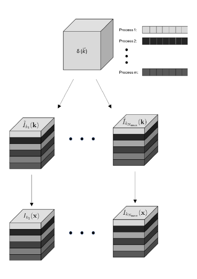
Figure 1: A visualization of the decomposition scheme. From the Fourier space density contrast field δ(𝒌)𝛿𝒌\delta({\bm{k}}), we construct Nmaxsubscript𝑁maxN_{\rm max} Fourier data cubes I~ki(𝒌)subscript~𝐼subscript𝑘𝑖𝒌\tilde{I}_{k_{i}}({\bm{k}}) for i=1𝑖1i=1 to Nmaxsubscript𝑁maxN_{\rm max} and distribute the array to m𝑚m different processes depicted as different gray scale colors. The data cubes I~ki(𝒌)subscript~𝐼subscript𝑘𝑖𝒌\tilde{I}_{k_{i}}({\bm{k}}) are spread out over each process such that each one only has access to a single contiguous chunk of one index and the full range of the others. For example, the first process stores I~ki(kF:k1max,kF:kmax,kF:kmax)\tilde{I}_{k_{i}}(k_{F}:k_{\rm 1max},k_{F}:k_{\rm max},k_{F}:k_{\rm max}) from all I~k1subscript~𝐼subscript𝑘1\tilde{I}_{k_{1}} to I~kNmaxsubscript~𝐼subscript𝑘subscript𝑁max\tilde{I}_{k_{N_{\rm max}}}. In this distribution scheme, the integration in Eq. (9) is done mostly in each local process, and the inter-CPU communication is only required at the last moment when we compute the total sum.

The key to the efficient parallelization of the polyspectra estimator is minimizing the inter-CPU communication, and we achieve that by using the slab decomposition scheme.

The slab decomposition slices the data cube along a single dimension, generally the fastest varying index, and assigns each chunk to different process. As each process stores a full range of other dimensions and limited range of the sliced dimension, this separates the data into ‘slabs’ of the domain hence the name slab decomposition. We show a visualization of this decomposition in Fig. 1. For the specific case of the polyspectra estimator, this decomposition takes the form of decomposing along the fastest varying Fourier grid dimension while the other two grid dimensions and the wavenumber dimension remain fully accessible in each process. For example, for the Julia implementation, we assign each process I~ki(k1min:k1max,kF:kmax,kF:kmax)\tilde{I}_{k_{i}}(k_{1\rm min}:k_{1\rm max},k_{\rm F}:k_{\rm max},k_{\rm F}:k_{\rm max}), and for C implementation, we assign each process I~ki(kF:kmax,kF:kmax,k3min:k3max)\tilde{I}_{k_{i}}(k_{\rm F}:k_{\rm max},k_{\rm F}:k_{\rm max},k_{3\rm min}:k_{3\rm max}) for all i𝑖i from 1 to Nmaxsubscript𝑁maxN_{\rm max}.

The choice of slab decomposition makes reading data from a file very memory efficient as the main process can send data to the other processes partway through reading the data by simply sending each slab to the proper process as it is read in, or by having each process read in their own slab of data. This also means that at no point does the reading process need more than a single slab of data at once in memory which helps to keep the maximum memory usage low. This memory distribution is also natural for the Fourier transformation as FFTW (Frigo & Johnson, 2005) implements distributed Fourier transforms through slab decomposition and transposing, allowing for a very natural calculation without need to shuffle around memory between processes to get the right format. The only other step in the calculation is the product and sum, the product is always able to be done locally within each process and the sum is a trivially parallizable calculation with very little extra memory usage or communication as each processes calculates a local sum before the main processes collects and finalizes the sum. All together this memory distribution scheme allows us to easily and quickly calculate this estimator with minimal memory footprint and very little inter-CPU communication.

This method must be contrasted with the naïve parallelization that each process contains the full I~ki(𝒌)subscript~𝐼subscript𝑘𝑖𝒌\tilde{I}_{k_{i}}({\bm{k}}) and Iki(𝒙)subscript𝐼subscript𝑘𝑖𝒙I_{k_{i}}(\bm{x}) for each wavenumber bin kisubscript𝑘𝑖k_{i}. For this alternative case, however, the time saved in the Fourier transform step is dwarfed by the significantly more expensive final step where we calculate sums of products across wavenumbers. As a result, this somewhat more natural decomposition is significantly slower than the slab decomposition.

4 Code Tests

In order to test the accuracy and performance of our implementation of the parallel estimator, we compute the number of polygons satisfying the homogeneity condition and the binning condition:

Nnpoly=subscript𝑁𝑛polyabsent\displaystyle N_{n\rm-poly}= Vn~Vfn1subscript𝑉~𝑛superscriptsubscript𝑉𝑓𝑛1\displaystyle\frac{V_{\tilde{n}}}{V_{f}^{n-1}}
=\displaystyle= 1kF3n3k1d3q1knd3qnδD(𝐪1n),1superscriptsubscript𝑘𝐹3𝑛3subscriptsubscript𝑘1superscript𝑑3subscript𝑞1subscriptsubscript𝑘𝑛superscript𝑑3subscript𝑞𝑛subscript𝛿𝐷subscript𝐪1𝑛\displaystyle\frac{1}{k_{F}^{3n-3}}\int_{k_{1}}d^{3}q_{1}\cdots\int_{k_{n}}d^{3}q_{n}\delta_{D}(\mathbf{q}_{1\cdots n}), (14)

for which we have present an analytical estimation (see Sec. 4.1 for the detail). Here, Vfsubscript𝑉𝑓V_{f} is the volume of the fundamental cell in the Fourier space, which is related to the fundamental Fourier wavenumber kFsubscript𝑘𝐹k_{F} by Vf=kF3subscript𝑉𝑓superscriptsubscript𝑘𝐹3V_{f}=k_{F}^{3}.

In practice, we estimate the number of polygons by setting δ(𝒌)=1𝛿𝒌1\delta({\bm{k}})=1 for all Fourier modes and estimating the angle-averaged polyspectra. Therefore, counting the number of polygons requires exactly the same procedure as estimating the polyspectra.

4.1 Number of Polygons

To obtain the number of n𝑛n-gons satisfying the binning conditions, we need to evaluate the 3n3𝑛3n-dimensional integration in Eq. (14). Again, using the Fourier representation of the Dirac-delta operator, we reduce the problem to the three-dimensional integration of multiplications of ιk(𝒙)subscript𝜄𝑘𝒙\iota_{k}(\bm{x}) (Eq. (11)), which is

ιk=kd3qei𝒒𝒙=4πk2(sin(kx)kx)δk+𝒪(δk3).subscript𝜄𝑘subscript𝑘superscript𝑑3𝑞superscript𝑒𝑖𝒒𝒙4𝜋superscript𝑘2𝑘𝑥𝑘𝑥𝛿𝑘𝒪𝛿superscript𝑘3\iota_{k}=\int_{k}d^{3}qe^{i\bm{q}\cdot\bm{x}}=4\pi k^{2}\left(\frac{\sin(kx)}{kx}\right)\delta k+{\mathcal{O}}(\delta k^{3})\,. (15)

Using the expression to leading order in the bin size δk𝛿𝑘\delta k, we further reduce the calculation of the 3n3𝑛3n-dimensional volume to the one-dimensional integration:

Vn~=subscript𝑉~𝑛absent\displaystyle V_{\tilde{n}}= d3x(2π)3i=1nιki(x)superscript𝑑3𝑥superscript2𝜋3superscriptsubscriptproduct𝑖1𝑛subscript𝜄subscript𝑘𝑖𝑥\displaystyle\int\frac{d^{3}x}{(2\pi)^{3}}\prod_{i=1}^{n}\iota_{k_{i}}(x)
=\displaystyle= (4πδk)n0dx2π2xn2i=1nkisin(kix).superscript4𝜋𝛿𝑘𝑛superscriptsubscript0𝑑𝑥2superscript𝜋2superscript𝑥𝑛2superscriptsubscriptproduct𝑖1𝑛subscript𝑘𝑖subscript𝑘𝑖𝑥\displaystyle(4\pi\delta k)^{n}\int_{0}^{\infty}\frac{dx}{2\pi^{2}x^{n-2}}\prod_{i=1}^{n}k_{i}\sin(k_{i}x)\,. (16)

In App. B, We find a general expression for the radial integration,

0dxxn2i=1nsin(kix)=π2(i=3nkikidκi2)superscriptsubscript0𝑑𝑥superscript𝑥𝑛2superscriptsubscriptproduct𝑖1𝑛subscript𝑘𝑖𝑥𝜋2superscriptsubscriptproduct𝑖3𝑛superscriptsubscriptsubscript𝑘𝑖subscript𝑘𝑖𝑑subscript𝜅𝑖2\displaystyle\int_{0}^{\infty}\frac{dx}{x^{n-2}}\prod_{i=1}^{n}\sin(k_{i}x)=\frac{\pi}{2}\left(\prod_{i=3}^{n}\int_{-k_{i}}^{k_{i}}\frac{d\kappa_{i}}{2}\right)
×[δD(i=3nκi+k1k2)δD(i=3nκik1k2)],absentdelimited-[]superscript𝛿𝐷superscriptsubscript𝑖3𝑛subscript𝜅𝑖subscript𝑘1subscript𝑘2superscript𝛿𝐷superscriptsubscript𝑖3𝑛subscript𝜅𝑖subscript𝑘1subscript𝑘2\displaystyle\times\left[\delta^{D}\left(\sum_{i=3}^{n}\kappa_{i}+k_{1}-k_{2}\right)-\delta^{D}\left(\sum_{i=3}^{n}\kappa_{i}-k_{1}-k_{2}\right)\right]\,, (17)

and apply Eq. (17) for n=3𝑛3n=3 and n=4𝑛4n=4 cases to find the number of triangles and quadrilaterals, which are given by

Ntri=1kF6{4π2k1k2k3(δk)3,k1=k2+k38π2k1k2k3(δk)3,k1<k2+k3,N_{\rm tri}=\frac{1}{k_{F}^{6}}\left\{\begin{array}[]{cc}4\pi^{2}k_{1}k_{2}k_{3}\left(\delta k\right)^{3}&,~{}k_{1}=k_{2}+k_{3}\\ 8\pi^{2}k_{1}k_{2}k_{3}\left(\delta k\right)^{3}&,~{}k_{1}<k_{2}+k_{3}\end{array}\right.\,, (18)

and

Nquad=subscript𝑁quadabsent\displaystyle N_{\rm quad}= 1kF98π3(δk)4k1k2k3k4(k1+k2+k3\displaystyle\frac{1}{k_{F}^{9}}8\pi^{3}\left(\delta k)^{4}k_{1}k_{2}k_{3}k_{4}(-k_{1}+k_{2}+k_{3}\right.
+3k4|k1k2k3+k4|).\displaystyle\left.+3k_{4}-|k_{1}-k_{2}-k_{3}+k_{4}|\right)\,. (19)

4.2 Result

Refer to caption
Refer to caption
Refer to caption
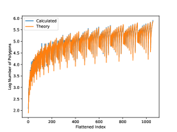
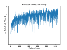
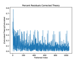
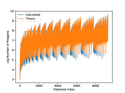
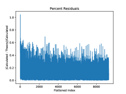
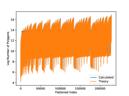
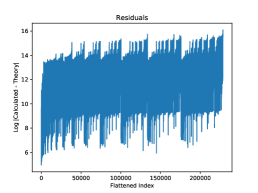
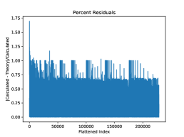
Figure 2: Left: The number of triangles satisfying the binning conditions measured from the parallel bispectrum estimator. The blue curve is the output from the numerical estimation, and the orange curve is according to our analytical estimation in Eq. (18) (see App. B for the derivation). Middle: The difference between the numerical measurement and theoretical estimation. Right: The fractional difference between the two. Besides the largest-scales (earlier indices) that we expect the analytical estimation breaks down, the analytical estimation in Eq. (18) is good to about 20%percent2020~{}\% accuracy.
Refer to caption
Refer to caption
Refer to caption
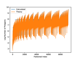
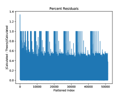
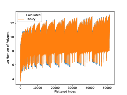
Figure 3: Left: The number of quadrilaterals satisfying the binning conditions measured from the parallel trispectrum estimator. The blue curve is the output from the numerical estimation, and the orange curve is according to our analytical estimation in Eq. (19). Middle: The same numerical result (blue) along with the improved analytical calculation, using exact expression for ιk(x)subscript𝜄𝑘𝑥\iota_{k}(x) (see, Eq. (B27)) and calculate the correction for the co-linear quadrilaterals as in Eq. (B29). Right: The fractional difference between the two curves in the middle panel. The small-scale (large wavenumber) discrepancies are consistently about 40%percent4040~{}\%.

In this section, we shall present number of polygons that we calculated using the parallelized polyspectra estimator and compare the result with the analytical estimation that we find in Sec. 4.1. We shall show the result for triangles (n=3𝑛3n=3), quadrilaterals (n=4𝑛4n=4), pentagons (n=5𝑛5n=5), and hexagons (n=6𝑛6n=6) that are estimated using, respectively, the parallel estimators of bispectrum, trispectrum, quadspectrum, and pentaspectrum.

To show the full shape dependence of the number of polygons as a function of their side length (wavenumbers), we need to visualize them in n𝑛n-dimensional space of (k1,k2,,kn)subscript𝑘1subscript𝑘2subscript𝑘𝑛(k_{1},k_{2},\cdots,k_{n}). For our purpose, however, to compare the outcome of the parallel computation and analytical estimation, it suffices to flatten n𝑛n-dimensional data points to the one-dimensional ordered sequence. Following the convention in McCullagh et al. (2016), we impose the condition kiki+1subscript𝑘𝑖subscript𝑘𝑖1k_{i}\geq k_{i+1} to avoid duplication and form the sequence by taking the row-major order of the n𝑛n-dimensional points (knsubscript𝑘𝑛k_{n} is the fastest varying dimension).

In all comparison plots that we present here, the x𝑥x axes show the index of the n𝑛n-dimensional point (k1,,kn)subscript𝑘1subscript𝑘𝑛(k_{1},\cdots,k_{n}) in the flattened sequence, and y𝑦y axes show the number of polygons whose n𝑛n sides are (k1,,kn)subscript𝑘1subscript𝑘𝑛(k_{1},\cdots,k_{n}). We use blue color to show the numerical result and orange color to show the analytical estimation.

First, we show the number of triangles using the parallel bispectrum estimator in Fig. 2. The left panel shows the numerical result (blue) and analytical prediction (Eq. (18)), while the middle and right panels show the absolute number (middle) and fractional (right) differences. On large scales (or small indices), we expect the analytical estimation is not accurate because the bin’s size is of order the wavenumber (kiδksimilar-to-or-equalssubscript𝑘𝑖𝛿𝑘k_{i}\simeq\delta k). For small scales, although the absolute residuals increases with wavenumbers (the lowest order error term goes as kiproductsubscript𝑘𝑖\prod k_{i} just like the Ntrisubscript𝑁triN_{\rm tri} in Eq. (18)), the fractional residual between the numerical and analytical estimation are consistently off by 1020%similar-to10percent2010\sim 20\%, and the biggest differences happen for the folded triangles (k1=k2+k3subscript𝑘1subscript𝑘2subscript𝑘3k_{1}=k_{2}+k_{3}). This result suggests that the variance of bispectrum estimated by using Eq. (18) (for example, in the Fisher information forecast in Desjacques et al. (2018)) must be off by the same factor. For an accurate estimation of the variance of the bispectrum, one must use the numerically estimated number of triangles.
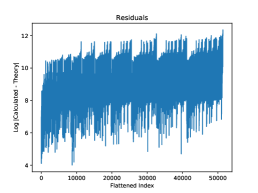
Refer to caption
Refer to caption
Refer to caption
Figure 4: The flattened number of pentagons/Angle Averaged Quadspectrum of unity. The orange is according to the number predicted by App. B and the blue curve is the output of the estimator run on a grid of unity on a spherical shell. The Quadspectrum shows very similar error behaviour to the Trispectrum and for much the same reasons cannot be practically used when calculating actual Quadspectrum.
Refer to caption
Refer to caption
Refer to caption
Figure 5: The flattened number of hexagons/Angle Averaged Pentaspectrum of unity. The orange is according to the number predicted by App. B and the blue curve is the output of the estimator run on a grid of unity on a spherical shell. The Pentaspectrum displays near identical error behaviour to the other high order polyspectra.

We perform the same analysis for the number of quadraliterals by using the parallel estimator for trispectrum. The left panel of Fig. 3 shows the comparison between the numerical result and the analytical estimation in Eq. (19). It turns out that biggest the discrepancies are for the co-linear quadrilaterals (k1=k2+k3+k4subscript𝑘1subscript𝑘2subscript𝑘3subscript𝑘4k_{1}=k_{2}+k_{3}+k_{4}) where the analytical formula, Eq. (19), predicts zero. To remedy the situation, we add the exact corrections for the co-linear quadrilaterals, Eq. (B29), and the analytical estimate indeed matches the numerical calculation better, as shown in the middle panel of Fig. 3.

We can easily extend the parallel estimator for the bispectrum and trispectrum to measure any n>4𝑛4n>4 polyspectra. We extend the estimator to n=5𝑛5n=5 and n=6𝑛6n=6 order polyspectra, and show the result in Fig. 4 and Fig. 5, respectively. In all cases the fractional errors between numerical calculation and analytical estimate are dominated by a collection of 100% error terms. These occur, just as the co-linear case for the quadrilaterals, because the leading-order approximation in the analytical calculation yields zeros when the actual calculation yields small but not-zero numbers. This happens for all n>4𝑛4n>4 cases, and it further reinforces the need for manually calculating the number of polygons when estimating the polyspectra, or estimating their variance.

4.3 Code performance

In this section, we present the performance of the parallel algorithm. All of our benchmarking work was done with 2.2 GHz Intel Xeon Processors on nodes with 40 CPU/node, 1 TB of RAM, 10 Gbps Ethernet and FDR Infiniband.

We have implemented two versions of parallel bispectrum estimator, one using C and the other using Julia. These two pieces of software perform the same algorithm. In Fig. 6, we compare the performance of the two implementations. Overall, as a function of domain length, the size of one-dimensional Fourier grid N𝑁N and the maximum wavenumber Nmax=kmax/kFsubscript𝑁maxsubscript𝑘maxsubscript𝑘𝐹N_{\rm max}=k_{\rm max}/k_{F}, the performance scales as 𝒪(N3Nmaxn)𝒪superscript𝑁3superscriptsubscript𝑁max𝑛\mathcal{O}(N^{3}N_{\rm max}^{n}), as we have analyzed in Sec. 2. If we apply the aliasing condition which requires that N>nNmax𝑁𝑛subscript𝑁maxN>nN_{\rm max} we can rewrite the scaling as 𝒪(n3Nmaxn+3)𝒪superscript𝑛3superscriptsubscript𝑁max𝑛3\mathcal{O}(n^{3}N_{\rm max}^{n+3}).

The C implementation (blue) out performs the Julia implementation (orange) for all domain lengths. The improvement, however, stays constant at about 30 seconds offset for reasonable grid sizes. As it is easier to read and modify the Julia version, we have extended the software to higher order polyspectra estimator only using Julia.

Refer to caption
Figure 6: The total time spent calculating the Bispectrum versus the length of one grid dimension for 40 processors. It roughly follows the 𝒪(N3)𝒪superscript𝑁3\mathcal{O}(N^{3}) you would expected given the sum in the algorithm with fixed Nmaxsubscript𝑁maxN_{\rm max}, modulo the overhead dominated small grid sizes. Each grid size was tested 50 times and then averaged. While the Julia version is slightly slower than the C version, the time difference is relatively consistent with around a constant 30 second offset for small grid sizes and is mostly negligible for large grid sizes given the overall length of the computation.

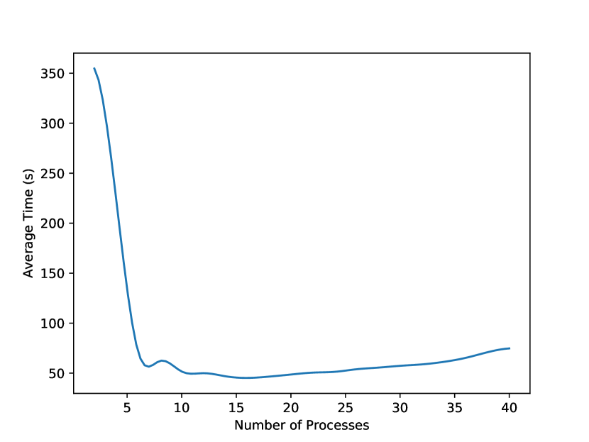
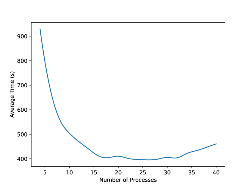
Fig. 7 shows the performance of our Julia implementation as a function of number of processors. Here, we use the domain size of N=256𝑁256N=256 (left panel) and N=512𝑁512N=512 (right panel). Initially, adding more CPUs improves the performance and reduces the execution time, but the improvement stops at some point. In fact, when the grid size per CPU is sufficiently small then adding more processes actually slows down the performance; the increased overhead time cancels the small gains in extra discretization.

How long does it take to estimate the bispectrum? In order to avoid the aliasing effect, the grid size must satisfy N>3Nmax𝑁3subscript𝑁maxN>3N_{\rm max} for estimating the bispectrum. Therefore, probing the bispectrum up to Nmax340similar-to-or-equalssubscript𝑁max340N_{\rm max}\simeq 340 requires the one-dimensional Fourier grid of N=1024𝑁1024N=1024; we can estimate the bispectrum in 20 minutes using 40 cores.

For a more concrete example, the HETDEX survey (Hill et al., 2008) has kF0.0045subscript𝑘𝐹0.0045k_{F}\approx 0.0045 hh/Mpc. Measuring the galaxy bispectrum to kmax=0.2subscript𝑘max0.2k_{\rm max}=0.2 hh/Mpc only requires Nmax=45subscript𝑁𝑚𝑎𝑥45N_{max}=45. With the parallel version of Scoccimarro estimator, we can measure the galaxy bispectrum for HETDEX in similar-to\sim40 seconds with 2 GB of memory distributed over 40 processors. Here, we did not run the in-place FFTW, and kept both Iki(𝒙)subscript𝐼subscript𝑘𝑖𝒙I_{k_{i}}(\bm{x}) and I~ki(𝒒)subscript~𝐼subscript𝑘𝑖𝒒\tilde{I}_{k_{i}}(\bm{q}). Similarly, WFIRST (Spergel et al., 2015) has kF0.0028subscript𝑘𝐹0.0028k_{F}\approx 0.0028 hh/Mpc corresponding to Nmax=75subscript𝑁max75N_{\rm max}=75 for kmax=0.2subscript𝑘max0.2k_{\rm max}=0.2 hh/Mpc. For our implementation over 40 processors this corresponds to similar-to\sim50 seconds and 11 GB of memory distributed over 40 processors to calculate the galaxy bispectrum for WFIRST.

With the scaling that we have discussed in Sec. 2, we can extend the previous example to find a general relationship. For a cosmological survey with volume V𝑉V and maximum wavenumber kmaxsubscript𝑘maxk_{\rm max}, we calculate the number of one-dimensional sampling point as

Nmax=kmaxkF=12πkmaxV1/3.subscript𝑁maxsubscript𝑘maxsubscript𝑘𝐹12𝜋subscript𝑘maxsuperscript𝑉13N_{\rm max}=\frac{k_{\rm max}}{k_{F}}=\frac{1}{2\pi}k_{\rm max}V^{1/3}\,. (20)

Because the performance of the Scoccimarro estimator scales as 𝒪(Nmax6)𝒪superscriptsubscript𝑁max6\mathcal{O}(N_{\rm max}^{6}), the estimated computing time becomes

tBispec40(kmax0.2h/Mpc)6(V2.7 Gpc3/h3)2sec,subscript𝑡𝐵𝑖𝑠𝑝𝑒𝑐40superscriptsubscript𝑘max0.2Mpc6superscript𝑉2.7superscript Gpc3superscript32sect_{Bispec}\approx 40\left(\frac{k_{\rm max}}{0.2h/\text{Mpc}}\right)^{6}\left(\frac{V}{2.7\text{ Gpc}^{3}/h^{3}}\right)^{2}\text{sec}, (21)

over 40 processors. For the higher-order polyspectra, we can extend this relationship by

tPnn327(kmax0.2h/Mpc)n+3(V2.7 Gpc3/h3)(n+3)/3min,similar-tosubscript𝑡𝑃𝑛superscript𝑛327superscriptsubscript𝑘max0.2Mpc𝑛3superscript𝑉2.7superscript Gpc3superscript3𝑛33mint_{Pn}\sim\frac{n^{3}}{27}\left(\frac{k_{\rm max}}{0.2h/\text{Mpc}}\right)^{n+3}\left(\frac{V}{2.7\text{ Gpc}^{3}/h^{3}}\right)^{(n+3)/3}\text{min}, (22)

again, over the 40 processors. This relationship matches with the execution time for the polyspectra that we have measured for generating the figures in this paper.
Refer to captionRefer to caption

Figure 7: Left: The scaling of an N=256 length grid over various numbers of processes. There is clear gains when initially increasing the number of processes but at a certain point overhead begins to dominate causing a slight slowdown. Right: The scaling of an N=512 length grid over various numbers of processes. It clearly takes a much larger number of processes to reach maximum efficiency, and is fast for larger number of processes. This scaling continues as grid size increases, meaning for reasonable grid sizes and number of processes it should be maximally efficient. Each number of processes was tested 50 times and then averaged.

5 Conclusion

In this paper, we present a novel parallel algorithm for estimating polyspectra of a complex field given on three-dimensional regular grids. While inheriting the efficiency of the Scoccimarro estimator, the parallel algorithm alleviates its rather stringent memory requirement by distributing the array into multiple processors. In addition, the key for efficient parallization is the slab-decomposition scheme that maintains only low level of inter-CPU data communication, avoiding massive data transportation.

Although we have only presented the case for the monopole (angle-averaged) polyspectra as a function of their side lengths (that is, the wavenumbers kisubscript𝑘𝑖k_{i}), for estimating the redshift-space galaxy bispectrum, one can easily extend the method to the angular multipoles by applying the slab decomposition to the multipole-weighed fields δn(𝒒)subscript𝛿𝑛𝒒\delta_{n}(\bm{q}) as described in Scoccimarro (2015). Beyond the galaxy bispectrum, measuring the polyspectra with the full (3n𝑛n - 6)-parameter dependencies requires little more elaboration, as the calculation involves convolution instead of matrix inner product (Eq. (13)). We shall leave this as a future project.

With the Julia implementation, we have demonstrated that for the galaxy surveys such as HETDEX and WFIRST, we can estimate the galaxy bispectrum down to k0.2h/Mpcsimilar-to-or-equals𝑘0.2Mpck\simeq 0.2\,{h/{\rm Mpc}} in about a minute, and even higher-order polyspectra in less than an hour time scales. With these execution time scales, it is feasible to study the high-order polyspectra by directly measuring them from the massive mock galaxy catalogs (Monaco et al., 2013; Kitaura et al., 2014; Avila et al., 2015; Izard et al., 2016; Munari et al., 2017; Agrawal et al., 2017; Taruya et al., 2018). If it is not for their own sake, studying the galaxy trispectrum (the four-point correlation function in Fourier space) and the galaxy pentaspectrum (the six-point correlation function) shall certainly elucidate the study of covariance matrix for, respectively, the galaxy power spectrum and the galaxy bispectrum.

We have stored our Julia implementation for the n𝑛n-point polyspectra at (https://github.com/JosephTomlinson/PolyspectrumEstimator), and those who are interested in C implementation for the bispectrum estimator may contact the authors.

We thank Emiliano Sefusatti for useful discussion. DJ and JT were supported at Pennsylvania State University by NSF grant (AST-1517363) and NASA ATP program (80NSSC18K1103).

References

  • Agrawal et al. (2017) Agrawal, A., Makiya, R., Chiang, C.-T., et al. 2017, Journal of Cosmology and Astro-Particle Physics, 2017, 003
  • Avila et al. (2015) Avila, S., Murray, S. G., Knebe, A., et al. 2015, MNRAS, 450, 1856
  • Blake et al. (2011) Blake, C., Brough, S., Colless, M., et al. 2011, MNRAS, 415, 2876
  • de la Torre et al. (2013) de la Torre, S., Guzzo, L., Peacock, J. A., et al. 2013, A&A, 557, A54
  • Desjacques et al. (2018) Desjacques, V., Jeong, D., & Schmidt, F. 2018, Phys. Rep., 733, 1
  • Frigo & Johnson (2005) Frigo, M., & Johnson, S. G. 2005, Proceedings of the IEEE, 93, 216, special issue on “Program Generation, Optimization, and Platform Adaptation”
  • Gaztañaga et al. (2005) Gaztañaga, E., Norberg, P., Baugh, C. M., & Croton, D. J. 2005, MNRAS, 364, 620
  • Gil-Marín et al. (2015) Gil-Marín, H., Noreña, J., Verde, L., et al. 2015, MNRAS, 451, 539
  • Hill et al. (2008) Hill, G. J., Gebhardt, K., Komatsu, E., et al. 2008, in Astronomical Society of the Pacific Conference Series, Vol. 399, Panoramic Views of Galaxy Formation and Evolution, ed. T. Kodama, T. Yamada, & K. Aoki, 115
  • Izard et al. (2016) Izard, A., Crocce, M., & Fosalba, P. 2016, MNRAS, 459, 2327
  • Jeong (2010) Jeong, D. 2010, PhD thesis, University of Texas at Austin ¡EMAIL¿djeong@astro.as.utexas.edu¡/EMAIL¿
  • Kaiser (1987) Kaiser, N. 1987, Monthly Notices of the Royal Astronomical Society (ISSN 0035-8711), 227, 1
  • Kitaura et al. (2014) Kitaura, F. S., Yepes, G., & Prada, F. 2014, MNRAS, 439, L21
  • Marín (2011) Marín, F. 2011, ApJ, 737, 97
  • Marín et al. (2013) Marín, F. A., Blake, C., Poole, G. B., et al. 2013, MNRAS, 432, 2654
  • McBride et al. (2011a) McBride, C. K., Connolly, A. J., Gardner, J. P., et al. 2011a, ApJ, 726, 13
  • McBride et al. (2011b) —. 2011b, ApJ, 739, 85
  • McCullagh et al. (2016) McCullagh, N., Jeong, D., & Szalay, A. S. 2016, MNRAS, 455, 2945
  • Monaco et al. (2013) Monaco, P., Sefusatti, E., Borgani, S., et al. 2013, MNRAS, 433, 2389
  • Munari et al. (2017) Munari, E., Monaco, P., Sefusatti, E., et al. 2017, MNRAS, 465, 4658
  • Nichol et al. (2006) Nichol, R. C., Sheth, R. K., Suto, Y., et al. 2006, MNRAS, 368, 1507
  • Nishimichi et al. (2007) Nishimichi, T., Kayo, I., Hikage, C., et al. 2007, PASJ, 59, 93
  • Parkinson et al. (2012) Parkinson, D., Riemer-Sørensen, S., Blake, C., et al. 2012, Phys. Rev. D, 86, 103518
  • Pezzotta et al. (2017) Pezzotta, A., de la Torre, S., Bel, J., et al. 2017, A&A, 604, A33
  • Planck Collaboration (2016) Planck Collaboration. 2016, A&A, 594, A17
  • Reid et al. (2012) Reid, B. A., Samushia, L., White, M., et al. 2012, MNRAS, 426, 2719
  • Scoccimarro (2000) Scoccimarro, R. 2000, ApJ, 544, 597
  • Scoccimarro (2015) —. 2015, Phys. Rev. D, 92, 083532
  • Scoccimarro et al. (2001) Scoccimarro, R., Feldman, H. A., Fry, J. N., & Frieman, J. A. 2001, ApJ, 546, 652
  • Sefusatti (2005) Sefusatti, E. 2005, PhD thesis, New York University, New York, USA
  • Spergel et al. (2015) Spergel, D., Gehrels, N., Baltay, C., et al. 2015, arXiv e-prints, arXiv:1503.03757
  • Taruya et al. (2018) Taruya, A., Nishimichi, T., & Jeong, D. 2018, Phys. Rev. D, 98, 103532
  • Tegmark et al. (2006) Tegmark, M., Eisenstein, D. J., Strauss, M. A., et al. 2006, Phys. Rev. D, 74, 123507
  • Verde et al. (2002) Verde, L., Heavens, A. F., Percival, W. J., et al. 2002, MNRAS, 335, 432

Appendix A Polyspectrum Estimator in Discrete Fourier Transformation

In the main manuscript, we have presented the polyspectra estimator in an contiguous limit, as an integral form. In the practical implementation, we have converted the estimator into a discrete summation as we present here. For our discrete implementation, following the FFTW convention, we use the unnormalized Discrete Fourier Transform and explicitly pull out all normalization factors. For more details, authors refer to Chapter 7 of Jeong (2010). Here, we note the discrete version of variables by square bracket [𝒙]delimited-[]𝒙[\bm{x}].

Let us first summarize the continuous version of the polyspectra estimator. Starting with the integral form of the general estimator Eq. (9)

P~n(k1,kn)=VfVn~(2π)3k1d3q1knd3qnδD(𝐪1n)δ(𝐪i).subscript~𝑃𝑛subscript𝑘1subscript𝑘𝑛subscript𝑉𝑓subscript𝑉~𝑛superscript2𝜋3subscriptsubscript𝑘1superscript𝑑3subscript𝑞1subscriptsubscript𝑘𝑛superscript𝑑3subscript𝑞𝑛subscript𝛿𝐷subscript𝐪1𝑛product𝛿subscript𝐪𝑖\tilde{P}_{n}(k_{1}\cdots,k_{n})=\frac{V_{f}}{V_{\tilde{n}}(2\pi)^{3}}\int_{k_{1}}d^{3}q_{1}\cdots\int_{k_{n}}d^{3}q_{n}\delta_{D}(\mathbf{q}_{1\cdots n})\prod\delta(\mathbf{q}_{i})\,. (A1)

We convert the Dirac-delta operator into its Fourier representation form:

δD(x)=d3k(2π)3eikx,subscript𝛿𝐷𝑥superscriptsubscriptsuperscript𝑑3𝑘superscript2𝜋3superscript𝑒𝑖𝑘𝑥\delta_{D}(x)=\int\limits_{-\infty}^{\infty}\frac{d^{3}k}{(2\pi)^{3}}e^{ik\cdot x}\,, (A2)

which, when input back into the estimator, results in

P~n(k1,kn)=VfVn~(2π)3d3x(2π)3Iki(x),subscript~𝑃𝑛subscript𝑘1subscript𝑘𝑛subscript𝑉𝑓subscript𝑉~𝑛superscript2𝜋3superscript𝑑3𝑥superscript2𝜋3productsubscript𝐼subscript𝑘𝑖𝑥\tilde{P}_{n}(k_{1}\cdots,k_{n})=\frac{V_{f}}{V_{\tilde{n}}(2\pi)^{3}}\int\frac{d^{3}x}{(2\pi)^{3}}\prod I_{k_{i}}(x), (A3)

where

Iki(x)=kid3qiei𝒙𝒒iδ(𝒒i)=d3qiei𝒙𝒒iI~ki(𝒒i),subscript𝐼subscript𝑘𝑖𝑥subscriptsubscript𝑘𝑖superscript𝑑3subscript𝑞𝑖superscript𝑒𝑖𝒙subscript𝒒𝑖𝛿subscript𝒒𝑖superscript𝑑3subscript𝑞𝑖superscript𝑒𝑖𝒙subscript𝒒𝑖subscript~𝐼subscript𝑘𝑖subscript𝒒𝑖I_{k_{i}}(x)=\int_{k_{i}}d^{3}q_{i}e^{i\bm{x}\cdot\bm{q}_{i}}\delta(\bm{q}_{i})=\int d^{3}q_{i}e^{i\bm{x}\cdot\bm{q}_{i}}\tilde{I}_{k_{i}}(\bm{q}_{i})\,, (A4)

is the Fourier Transform of Iki(𝒒)subscript𝐼subscript𝑘𝑖𝒒I_{k_{i}}(\bm{q}) which is defined to be the same as δ(𝒒)𝛿𝒒\delta(\bm{q}) within a spherical shell with Fourier-space radius |𝒒|kisimilar-to-or-equals𝒒subscript𝑘𝑖|\bm{q}|\simeq k_{i}, and zero otherwise.

In the FFTW convention of un-normalized DFT, we find

Iki[𝒙]=(2π)3N3FFTW(I~ki[𝒒]),subscript𝐼subscript𝑘𝑖delimited-[]𝒙superscript2𝜋3superscript𝑁3FFTWsubscript~𝐼subscript𝑘𝑖delimited-[]𝒒I_{k_{i}}[\bm{x}]=\frac{(2\pi)^{3}}{N^{3}}{\rm FFTW}\left(\tilde{I}_{k_{i}}[\bm{q}]\right)\,, (A5)

with which we get a partially discretized estimator

P~n(k1,kn)=VfVn~(2π)3((2π)3N3)nd3x(2π)3i=1nFFTW(I~ki[𝒒]).subscript~𝑃𝑛subscript𝑘1subscript𝑘𝑛subscript𝑉𝑓subscript𝑉~𝑛superscript2𝜋3superscriptsuperscript2𝜋3superscript𝑁3𝑛superscript𝑑3𝑥superscript2𝜋3superscriptsubscriptproduct𝑖1𝑛FFTWsubscript~𝐼subscript𝑘𝑖delimited-[]𝒒\tilde{P}_{n}(k_{1}\cdots,k_{n})=\frac{V_{f}}{V_{\tilde{n}}(2\pi)^{3}}\left(\frac{(2\pi)^{3}}{N^{3}}\right)^{n}\int\frac{d^{3}x}{(2\pi)^{3}}\prod_{i=1}^{n}{\rm FFTW}\left(\tilde{I}_{k_{i}}[\bm{q}]\right)\,. (A6)

We then fully discretize the estimator by converting the final integral to a sum:

P~n(k1,kn)=subscript~𝑃𝑛subscript𝑘1subscript𝑘𝑛absent\displaystyle\tilde{P}_{n}(k_{1}\cdots,k_{n})= (Vfn1Vn~)(2π)3nVfn2N3nV(2π)6N3[𝒙]i=1nFFTW(I~ki[𝒒])superscriptsubscript𝑉𝑓𝑛1subscript𝑉~𝑛superscript2𝜋3𝑛superscriptsubscript𝑉𝑓𝑛2superscript𝑁3𝑛𝑉superscript2𝜋6superscript𝑁3subscriptdelimited-[]𝒙superscriptsubscriptproduct𝑖1𝑛FFTWsubscript~𝐼subscript𝑘𝑖delimited-[]𝒒\displaystyle\left(\frac{V_{f}^{n-1}}{V_{\tilde{n}}}\right)\frac{(2\pi)^{3n}}{V_{f}^{n-2}N^{3n}}\frac{V}{(2\pi)^{6}N^{3}}\sum\limits_{[\bm{x}]}\prod_{i=1}^{n}{\rm FFTW}\left(\tilde{I}_{k_{i}}[\bm{q}]\right)
=\displaystyle= (Vfn1Vn~)Vn1N3n1N3[𝒙]i=1nFFTW(I~ki[𝒒]).superscriptsubscript𝑉𝑓𝑛1subscript𝑉~𝑛superscript𝑉𝑛1superscript𝑁3𝑛1superscript𝑁3subscriptdelimited-[]𝒙superscriptsubscriptproduct𝑖1𝑛FFTWsubscript~𝐼subscript𝑘𝑖delimited-[]𝒒\displaystyle\left(\frac{V_{f}^{n-1}}{V_{\tilde{n}}}\right)\frac{V^{n-1}}{N^{3n}}\frac{1}{N^{3}}\sum\limits_{[\bm{x}]}\prod_{i=1}^{n}{\rm FFTW}\left(\tilde{I}_{k_{i}}[\bm{q}]\right)\,. (A7)

Finally, the quantity in parenthesis Vfn1Vn~superscriptsubscript𝑉𝑓𝑛1subscript𝑉~𝑛\frac{V_{f}^{n-1}}{V_{\tilde{n}}} is the reciprocal of the number of polygons, and we can compute them by applying the same polyspectra estimator to a Fourier grid of unity. Note, however, that the normalization is different here.

Vn~Vfn1=1Vfn1k1d3q1knd3qnδD(𝐪1n)=1N3Vfn1[𝒙]i=1nFFTW(ι~ki[𝒒]).subscript𝑉~𝑛superscriptsubscript𝑉𝑓𝑛11superscriptsubscript𝑉𝑓𝑛1subscriptsubscript𝑘1superscript𝑑3subscript𝑞1subscriptsubscript𝑘𝑛superscript𝑑3subscript𝑞𝑛subscript𝛿𝐷subscript𝐪1𝑛1superscript𝑁3superscriptsubscript𝑉𝑓𝑛1subscriptdelimited-[]𝒙superscriptsubscriptproduct𝑖1𝑛FFTWsubscript~𝜄subscript𝑘𝑖delimited-[]𝒒\frac{V_{\tilde{n}}}{V_{f}^{n-1}}=\frac{1}{V_{f}^{n-1}}\int_{k_{1}}d^{3}q_{1}\cdots\int_{k_{n}}d^{3}q_{n}\delta_{D}(\mathbf{q}_{1\cdots n})=\frac{1}{N^{3}V_{f}^{n-1}}\sum_{[\bm{x}]}\prod_{i=1}^{n}{\rm FFTW}\left(\tilde{\iota}_{k_{i}}[\bm{q}]\right)\,. (A8)

where we define ι~ki[𝒒]subscript~𝜄subscript𝑘𝑖delimited-[]𝒒\tilde{\iota}_{k_{i}}[\bm{q}], analogous to I~ki[𝒒]subscript~𝐼subscript𝑘𝑖delimited-[]𝒒\tilde{I}_{k_{i}}[\bm{q}] above, as the Fourier grid which takes unity within the spherical shell bounded by |kki|<δk/2𝑘subscript𝑘𝑖𝛿𝑘2|k-k_{i}|<\delta k/2 and zero elsewhere.

Appendix B Approximate Analytic Number of Polygons

In the polyspectra estimator, we have the normalization constant Vn~Vfn1subscript𝑉~𝑛superscriptsubscript𝑉𝑓𝑛1\frac{V_{\tilde{n}}}{V_{f}^{n-1}}, which is the number of n𝑛n-gons that satisfy the closing condition (Dirac-delta) for a given set of side-length wavenumber kisubscript𝑘𝑖k_{i}. In this appendix, we shall present the analytical approximation to this quantity.

Using the Dirac-delta (Eq. (A2)), we rewrite the 3n3𝑛3n-dimensional volume Vn~subscript𝑉~𝑛V_{\tilde{n}} as

Vn~=k1d3q1knd3qnδD(𝐪1n)=1(2π)3𝑑x3k1d3q1ei𝐱𝐪1knd3qnei𝐱𝐪n,subscript𝑉~𝑛subscriptsubscript𝑘1superscript𝑑3subscript𝑞1subscriptsubscript𝑘𝑛superscript𝑑3subscript𝑞𝑛subscript𝛿𝐷subscript𝐪1𝑛1superscript2𝜋3differential-dsuperscript𝑥3subscriptsubscript𝑘1superscript𝑑3subscript𝑞1superscript𝑒𝑖𝐱subscript𝐪1subscriptsubscript𝑘𝑛superscript𝑑3subscript𝑞𝑛superscript𝑒𝑖𝐱subscript𝐪𝑛V_{\tilde{n}}=\int_{k_{1}}d^{3}q_{1}\cdots\int_{k_{n}}d^{3}q_{n}\delta_{D}(\mathbf{q}_{1\cdots n})=\frac{1}{(2\pi)^{3}}\int dx^{3}\int_{k_{1}}d^{3}q_{1}e^{i\mathbf{x}\cdot\mathbf{q}_{1}}\cdots\int_{k_{n}}d^{3}q_{n}e^{i\mathbf{x}\cdot\mathbf{q}_{n}}\,, (B1)

for which we can compute the each qisubscript𝑞𝑖q_{i} integration as

kd3qei𝐪𝐱=4πkδk/2k+δk/2𝑑qq2sin(qx)qx4πksin(kx)xδk+𝒪(δk3).subscript𝑘superscript𝑑3𝑞superscript𝑒𝑖𝐪𝐱4𝜋subscriptsuperscript𝑘𝛿𝑘2𝑘𝛿𝑘2differential-d𝑞superscript𝑞2𝑞𝑥𝑞𝑥4𝜋𝑘𝑘𝑥𝑥𝛿𝑘𝒪𝛿superscript𝑘3\int_{k}d^{3}qe^{i\mathbf{q}\cdot\mathbf{x}}=4\pi\int\limits^{k+\delta k/2}_{k-\delta k/2}dqq^{2}\frac{\sin(qx)}{qx}\approx 4\pi\frac{k\sin(kx)}{x}\delta k+\mathcal{O}(\delta k^{3}). (B2)

Combining the two results, we reduce the number of n𝑛n-gons to one-dimensional integration as

Vn~=22n3πn3(i=1nkiδk)d3x1xni=1nsin(kix)=22n1πn2(i=1nkiδk)0dxxn2i=1nsin(kix).subscript𝑉~𝑛superscript22𝑛3superscript𝜋𝑛3superscriptsubscriptproduct𝑖1𝑛subscript𝑘𝑖𝛿𝑘superscript𝑑3𝑥1superscript𝑥𝑛superscriptsubscriptproduct𝑖1𝑛subscript𝑘𝑖𝑥superscript22𝑛1superscript𝜋𝑛2superscriptsubscriptproduct𝑖1𝑛subscript𝑘𝑖𝛿𝑘superscriptsubscript0𝑑𝑥superscript𝑥𝑛2superscriptsubscriptproduct𝑖1𝑛subscript𝑘𝑖𝑥V_{\tilde{n}}=2^{2n-3}\pi^{n-3}\left(\prod_{i=1}^{n}k_{i}\delta k\right)\int d^{3}x\frac{1}{x^{n}}\prod_{i=1}^{n}\sin\left(k_{i}x\right)=2^{2n-1}\pi^{n-2}\left(\prod_{i=1}^{n}k_{i}\delta k\right)\int\limits_{0}^{\infty}\frac{dx}{x^{n-2}}\prod_{i=1}^{n}\sin\left(k_{i}x\right)\,. (B3)

which is an analytically tractable integral, given the assumptions that kiki+1subscript𝑘𝑖subscript𝑘𝑖1k_{i}\geq k_{i+1} (to uniquely define the polygon), and the polygon condition that (ijki)kjsubscript𝑖𝑗subscript𝑘𝑖subscript𝑘𝑗(\sum_{i\neq j}k_{i})\geq k_{j}.

In what follows, we shall show the calculations. First, we show the general strategy of integrating nsubscript𝑛{\cal I}_{n} in App. B.1, which is followed by the explicit result for n=3𝑛3n=3 (App. B.2) and n=4𝑛4n=4 (App. B.3) cases. We then present the calculation for the colinear case, k1=k2++knk_{1}=k_{2}+\cdot+k_{n}, where the approximation in Eq. (B2) resulting zero for all n>4𝑛4n>4 polygons. We therefore show the explicit expression without approximation in Eq. (B2) in App. B.4.

B.1 The analytical calculation: general case

To simplify the notation, let us define following function

n(k1,,kn)0𝑑xsin(kix)xn2=12dxxn2i=1nsin(kix),subscript𝑛subscript𝑘1subscript𝑘𝑛superscriptsubscript0differential-d𝑥productsubscript𝑘𝑖𝑥superscript𝑥𝑛212superscriptsubscript𝑑𝑥superscript𝑥𝑛2superscriptsubscriptproduct𝑖1𝑛subscript𝑘𝑖𝑥{\cal I}_{n}\left(k_{1},\cdots,k_{n}\right)\equiv\int\limits_{0}^{\infty}dx\frac{\prod\sin(k_{i}x)}{x^{n-2}}=\frac{1}{2}\int_{-\infty}^{\infty}\frac{dx}{x^{n-2}}\prod_{i=1}^{n}\sin\left(k_{i}x\right), (B4)

where we use that the integrand is an even function of x𝑥x. Here, we show the general strategy of solving for the function nsubscript𝑛{\cal I}_{n}. First, we use the following identity:

sin(kx)kx=11dμ2eikxμ,𝑘𝑥𝑘𝑥superscriptsubscript11𝑑𝜇2superscript𝑒𝑖𝑘𝑥𝜇\frac{\sin(kx)}{kx}=\int_{-1}^{1}\frac{d\mu}{2}\,e^{ikx\mu}\,, (B5)

to transform the integration as

n(k1,,kn)=k1kn2dx211dμ1211dμn22eix(k1μ1++kn2μn2)sin(kn1x)sin(knx).subscript𝑛subscript𝑘1subscript𝑘𝑛subscript𝑘1subscript𝑘𝑛2superscriptsubscript𝑑𝑥2superscriptsubscript11𝑑subscript𝜇12superscriptsubscript11𝑑subscript𝜇𝑛22superscript𝑒𝑖𝑥subscript𝑘1subscript𝜇1subscript𝑘𝑛2subscript𝜇𝑛2subscript𝑘𝑛1𝑥subscript𝑘𝑛𝑥{\cal I}_{n}(k_{1},\cdots,k_{n})=k_{1}\cdots k_{n-2}\int_{-\infty}^{\infty}\frac{dx}{2}\int_{-1}^{1}\frac{d\mu_{1}}{2}\cdots\int_{-1}^{1}\frac{d\mu_{n-2}}{2}e^{ix\left(k_{1}\mu_{1}+\cdots+k_{n-2}\mu_{n-2}\right)}\sin\left(k_{n-1}x\right)\sin\left(k_{n}x\right)\,. (B6)

We then use

sin(kn1x)sin(knx)=subscript𝑘𝑛1𝑥subscript𝑘𝑛𝑥absent\displaystyle\sin\left(k_{n-1}x\right)\sin\left(k_{n}x\right)= 1(2i)2[eikn1xeikn1x][eiknxeiknx]1superscript2𝑖2delimited-[]superscript𝑒𝑖subscript𝑘𝑛1𝑥superscript𝑒𝑖subscript𝑘𝑛1𝑥delimited-[]superscript𝑒𝑖subscript𝑘𝑛𝑥superscript𝑒𝑖subscript𝑘𝑛𝑥\displaystyle\frac{1}{(2i)^{2}}\left[e^{ik_{n-1}x}-e^{-ik_{n-1}x}\right]\left[e^{ik_{n}x}-e^{-ik_{n}x}\right]
=\displaystyle= 14(ei(kn1kn)x+ei(kn1kn)xei(kn1+kn)xei(kn1+kn)x),14superscript𝑒𝑖subscript𝑘𝑛1subscript𝑘𝑛𝑥superscript𝑒𝑖subscript𝑘𝑛1subscript𝑘𝑛𝑥superscript𝑒𝑖subscript𝑘𝑛1subscript𝑘𝑛𝑥superscript𝑒𝑖subscript𝑘𝑛1subscript𝑘𝑛𝑥\displaystyle\frac{1}{4}\left(e^{i(k_{n-1}-k_{n})x}+e^{-i(k_{n-1}-k_{n})x}-e^{i(k_{n-1}+k_{n})x}-e^{-i(k_{n-1}+k_{n})x}\right)\,, (B7)

to convert the integrations in terms of the Dirac-delta operator:

δD(k)=dx2πeikx.superscript𝛿𝐷𝑘superscriptsubscript𝑑𝑥2𝜋superscript𝑒𝑖𝑘𝑥\delta^{D}(k)=\int_{-\infty}^{\infty}\frac{dx}{2\pi}e^{ikx}\,. (B8)

That is,

n(k1,,kn)=subscript𝑛subscript𝑘1subscript𝑘𝑛absent\displaystyle{\cal I}_{n}(k_{1},\cdots,k_{n})= π4k1kn211dμ1211dμn22𝜋4subscript𝑘1subscript𝑘𝑛2superscriptsubscript11𝑑subscript𝜇12superscriptsubscript11𝑑subscript𝜇𝑛22\displaystyle\frac{\pi}{4}k_{1}\cdots k_{n-2}\int_{-1}^{1}\frac{d\mu_{1}}{2}\cdots\int_{-1}^{1}\frac{d\mu_{n-2}}{2}
×[δD(k1μ1++kn2μn2+kn1kn)+δD(k1μ1++kn2μn2kn1+kn)\displaystyle\times\Biggl{[}\delta^{D}\left(k_{1}\mu_{1}+\cdots+k_{n-2}\mu_{n-2}+k_{n-1}-k_{n}\right)+\delta^{D}\left(k_{1}\mu_{1}+\cdots+k_{n-2}\mu_{n-2}-k_{n-1}+k_{n}\right)
δD(k1μ1++kn2μn2+kn1+kn)δD(k1μ1++kn2μn2kn1kn)]\displaystyle\qquad-\delta^{D}\left(k_{1}\mu_{1}+\cdots+k_{n-2}\mu_{n-2}+k_{n-1}+k_{n}\right)-\delta^{D}\left(k_{1}\mu_{1}+\cdots+k_{n-2}\mu_{n-2}-k_{n-1}-k_{n}\right)\Biggl{]}
=\displaystyle= π2k1kn211dμ1211dμn22𝜋2subscript𝑘1subscript𝑘𝑛2superscriptsubscript11𝑑subscript𝜇12superscriptsubscript11𝑑subscript𝜇𝑛22\displaystyle\frac{\pi}{2}k_{1}\cdots k_{n-2}\int_{-1}^{1}\frac{d\mu_{1}}{2}\cdots\int_{-1}^{1}\frac{d\mu_{n-2}}{2}
×[δD(k1μ1++kn2μn2+kn1kn)δD(k1μ1++kn2μn2kn1kn)]\displaystyle\times\Biggl{[}\delta^{D}\left(k_{1}\mu_{1}+\cdots+k_{n-2}\mu_{n-2}+k_{n-1}-k_{n}\right)-\delta^{D}\left(k_{1}\mu_{1}+\cdots+k_{n-2}\mu_{n-2}-k_{n-1}-k_{n}\right)\Biggl{]}
=\displaystyle= π2k1k1dκ12kn2kn2dκn22[δD(κ1++κn2+kn1kn)δD(κ1++κn2kn1kn)].\displaystyle\frac{\pi}{2}\int_{-k_{1}}^{k_{1}}\frac{d\kappa_{1}}{2}\cdots\int_{-k_{n-2}}^{k_{n-2}}\frac{d\kappa_{n-2}}{2}\Biggl{[}\delta^{D}\left(\kappa_{1}+\cdots+\kappa_{n-2}+k_{n-1}-k_{n}\right)-\delta^{D}\left(\kappa_{1}+\cdots+\kappa_{n-2}-k_{n-1}-k_{n}\right)\Biggl{]}\,. (B9)

Going beyond this result requires the conditions to form polygons. For general polygons in 3D there is only one condition, the longest side must be less than or equal to the sum of all the other sides. If we don’t want to be bothered by the ordering, we can simply state as following: For any j[1,n]𝑗1𝑛j\in[1,n],

kjk1++kj1+kj+1++kn=i=1nkikj.subscript𝑘𝑗subscript𝑘1subscript𝑘𝑗1subscript𝑘𝑗1subscript𝑘𝑛superscriptsubscript𝑖1𝑛subscript𝑘𝑖subscript𝑘𝑗k_{j}\leq k_{1}+\cdots+k_{j-1}+k_{j+1}+\cdots+k_{n}=\sum_{i=1}^{n}k_{i}-k_{j}\,. (B10)

With this condition, we can see that there must be a solution for μi(0,1)subscript𝜇𝑖01\mu_{i}\in(0,1) satisfying

kn=k1μ1++kn2μn2+kn1.subscript𝑘𝑛subscript𝑘1subscript𝜇1subscript𝑘𝑛2subscript𝜇𝑛2subscript𝑘𝑛1k_{n}=k_{1}\mu_{1}+\cdots+k_{n-2}\mu_{n-2}+k_{n-1}\,. (B11)

For later use, we find following identity for the integration of the Dirac delta useful:

kk𝑑κδD(κa)=Θ(ka,k+a).superscriptsubscript𝑘𝑘differential-d𝜅superscript𝛿𝐷𝜅𝑎Θ𝑘𝑎𝑘𝑎\int_{-k}^{k}d\kappa\delta^{D}(\kappa-a)=\Theta(k-a,k+a). (B12)

Here Θ(x1,x2,,xn)Θsubscript𝑥1subscript𝑥2subscript𝑥𝑛\Theta(x_{1},x_{2},\cdot,x_{n}) is a multi-dimensional Heaviside-Theta function, which is 1 only if none of the xisubscript𝑥𝑖x_{i} are not positive.

B.2 The analytical calculation for triangles (n=3𝑛3n=3)

For the bispectrum (n=3𝑛3n=3), Eq. (B9) reduces to

3=subscript3absent\displaystyle{\cal I}_{3}= π2k1k1dκ12[δD(κ1+k2k3)δD(κ1k2k3)]𝜋2superscriptsubscriptsubscript𝑘1subscript𝑘1𝑑subscript𝜅12delimited-[]superscript𝛿𝐷subscript𝜅1subscript𝑘2subscript𝑘3superscript𝛿𝐷subscript𝜅1subscript𝑘2subscript𝑘3\displaystyle\frac{\pi}{2}\int_{-k_{1}}^{k_{1}}\frac{d\kappa_{1}}{2}\left[\delta^{D}(\kappa_{1}+k_{2}-k_{3})-\delta^{D}(\kappa_{1}-k_{2}-k_{3})\right]
=\displaystyle= π4[Θ(k1+k2k3,k1k2+k3)Θ(k1k2k3,k1+k2+k3)].𝜋4delimited-[]Θsubscript𝑘1subscript𝑘2subscript𝑘3subscript𝑘1subscript𝑘2subscript𝑘3Θsubscript𝑘1subscript𝑘2subscript𝑘3subscript𝑘1subscript𝑘2subscript𝑘3\displaystyle\frac{\pi}{4}\left[\Theta(k_{1}+k_{2}-k_{3},k_{1}-k_{2}+k_{3})-\Theta(k_{1}-k_{2}-k_{3},k_{1}+k_{2}+k_{3})\right]\,. (B13)

Without loss of generality, let us order the wavenumbers so that k1k2k3subscript𝑘1subscript𝑘2subscript𝑘3k_{1}\geq k_{2}\geq k_{3}. Then, from the polygon inequality in Eq. (B10), the first term becomes

Θ(k1+k2k3,k1k2+k3)=1,Θsubscript𝑘1subscript𝑘2subscript𝑘3subscript𝑘1subscript𝑘2subscript𝑘31\Theta(k_{1}+k_{2}-k_{3},k_{1}-k_{2}+k_{3})=1\,, (B14)

and the second term is

Θ(k1k2k3,k1+k2+k3)={1/2,k1=k2+k30,k1<k2+k3.\Theta(k_{1}-k_{2}-k_{3},k_{1}+k_{2}+k_{3})=\left\{\begin{array}[]{cc}1/2&,~{}k_{1}=k_{2}+k_{3}\\ 0&,~{}k_{1}<k_{2}+k_{3}\end{array}\right.\,. (B15)

Therefore,

3={π/8,k1=k2+k3π/4,k1<k2+k3,{\cal I}_{3}=\left\{\begin{array}[]{cc}\pi/8&,~{}k_{1}=k_{2}+k_{3}\\ \pi/4&,~{}k_{1}<k_{2}+k_{3}\end{array}\right.\,, (B16)

and

VB={4π2k1k2k3(δk)3,k1=k2+k38π2k1k2k3(δk)3,k1<k2+k3.V_{B}=\left\{\begin{array}[]{cc}4\pi^{2}k_{1}k_{2}k_{3}\left(\delta k\right)^{3}&,~{}k_{1}=k_{2}+k_{3}\\ 8\pi^{2}k_{1}k_{2}k_{3}\left(\delta k\right)^{3}&,~{}k_{1}<k_{2}+k_{3}\end{array}\right.\,. (B17)

B.3 The analytical calculation for trispectrum

For the trispectrum (n=4𝑛4n=4), Eq. (B9) reduces to

4=subscript4absent\displaystyle{\cal I}_{4}= π2k1k1dκ12k2k2dκ22[δD(κ1+κ2+k3k4)δD(κ1+κ2k3k4)]𝜋2superscriptsubscriptsubscript𝑘1subscript𝑘1𝑑subscript𝜅12superscriptsubscriptsubscript𝑘2subscript𝑘2𝑑subscript𝜅22delimited-[]superscript𝛿𝐷subscript𝜅1subscript𝜅2subscript𝑘3subscript𝑘4superscript𝛿𝐷subscript𝜅1subscript𝜅2subscript𝑘3subscript𝑘4\displaystyle\frac{\pi}{2}\int_{-k_{1}}^{k_{1}}\frac{d\kappa_{1}}{2}\int_{-k_{2}}^{k_{2}}\frac{d\kappa_{2}}{2}\left[\delta^{D}(\kappa_{1}+\kappa_{2}+k_{3}-k_{4})-\delta^{D}(\kappa_{1}+\kappa_{2}-k_{3}-k_{4})\right]
=\displaystyle= π4k1k1dκ12[Θ(k2+κ1+k3k4,k2κ1k3+k4)Θ(k2+κ1k3k4,k2κ1+k3+k4)].𝜋4superscriptsubscriptsubscript𝑘1subscript𝑘1𝑑subscript𝜅12delimited-[]Θsubscript𝑘2subscript𝜅1subscript𝑘3subscript𝑘4subscript𝑘2subscript𝜅1subscript𝑘3subscript𝑘4Θsubscript𝑘2subscript𝜅1subscript𝑘3subscript𝑘4subscript𝑘2subscript𝜅1subscript𝑘3subscript𝑘4\displaystyle\frac{\pi}{4}\int_{-k_{1}}^{k_{1}}\frac{d\kappa_{1}}{2}\left[\Theta(k_{2}+\kappa_{1}+k_{3}-k_{4},k_{2}-\kappa_{1}-k_{3}+k_{4})-\Theta(k_{2}+\kappa_{1}-k_{3}-k_{4},k_{2}-\kappa_{1}+k_{3}+k_{4})\right]\,. (B18)

Again, without loss of generality, we can order the wavenumbers so that k1k2k3k4subscript𝑘1subscript𝑘2subscript𝑘3subscript𝑘4k_{1}\geq k_{2}\geq k_{3}\geq k_{4}.

We first consider the case where k1=k2+k3+k4subscript𝑘1subscript𝑘2subscript𝑘3subscript𝑘4k_{1}=k_{2}+k_{3}+k_{4}. The integration then becomes

4=subscript4absent\displaystyle{\cal I}_{4}= π4k1k1dκ12[Θ(κ1+k12k4,κ1+k12k3)Θ(κ1+2k2k1,k1κ1)]𝜋4superscriptsubscriptsubscript𝑘1subscript𝑘1𝑑subscript𝜅12delimited-[]Θsubscript𝜅1subscript𝑘12subscript𝑘4subscript𝜅1subscript𝑘12subscript𝑘3Θsubscript𝜅12subscript𝑘2subscript𝑘1subscript𝑘1subscript𝜅1\displaystyle\frac{\pi}{4}\int_{-k_{1}}^{k_{1}}\frac{d\kappa_{1}}{2}\left[\Theta(\kappa_{1}+k_{1}-2k_{4},-\kappa_{1}+k_{1}-2k_{3})-\Theta(\kappa_{1}+2k_{2}-k_{1},k_{1}-\kappa_{1})\right]
=\displaystyle= π4[max(k1,k1+2k4)min(k1,k12k3)dκ12max(k1,k12k2)k1dκ12]=π8[k12k3(k1+2k4)(k1(k12k2))]=0.𝜋4delimited-[]superscriptsubscriptmaxsubscript𝑘1subscript𝑘12subscript𝑘4minsubscript𝑘1subscript𝑘12subscript𝑘3𝑑subscript𝜅12superscriptsubscriptmaxsubscript𝑘1subscript𝑘12subscript𝑘2subscript𝑘1𝑑subscript𝜅12𝜋8delimited-[]subscript𝑘12subscript𝑘3subscript𝑘12subscript𝑘4subscript𝑘1subscript𝑘12subscript𝑘20\displaystyle\frac{\pi}{4}\left[\int_{{\rm max}(-k_{1},-k_{1}+2k_{4})}^{{\rm min}(k_{1},k_{1}-2k_{3})}\frac{d\kappa_{1}}{2}-\int_{{\rm max}(-k_{1},k_{1}-2k_{2})}^{k_{1}}\frac{d\kappa_{1}}{2}\right]=\frac{\pi}{8}\left[k_{1}-2k_{3}-(-k_{1}+2k_{4})-(k_{1}-(k_{1}-2k_{2}))\right]=0\,. (B19)

That is, the number of trispectrum using Eq. (B2) vanishes for the colinear quadraliterals. We present the expression without using the approximation in App. B.4.

For the other cases, k1<k2+k3+k4subscript𝑘1subscript𝑘2subscript𝑘3subscript𝑘4k_{1}<k_{2}+k_{3}+k_{4}, we integrate 4subscript4{\cal I}_{4} as following. The first Heaviside-Theta function vanishes unless,

k2k3+k4κ1k2k3+k4,subscript𝑘2subscript𝑘3subscript𝑘4subscript𝜅1subscript𝑘2subscript𝑘3subscript𝑘4-k_{2}-k_{3}+k_{4}\leq\kappa_{1}\leq k_{2}-k_{3}+k_{4}, (B20)

so that we integrate the first term as

k1k1dκ12Θ(k2+κ1+k3k4,k2κ1k3+k4)=superscriptsubscriptsubscript𝑘1subscript𝑘1𝑑subscript𝜅12Θsubscript𝑘2subscript𝜅1subscript𝑘3subscript𝑘4subscript𝑘2subscript𝜅1subscript𝑘3subscript𝑘4absent\displaystyle\int_{-k_{1}}^{k_{1}}\frac{d\kappa_{1}}{2}\Theta(k_{2}+\kappa_{1}+k_{3}-k_{4},k_{2}-\kappa_{1}-k_{3}+k_{4})= max(k1,k2k3+k4)min(k1,k2k3+k4)dκ12superscriptsubscriptmaxsubscript𝑘1subscript𝑘2subscript𝑘3subscript𝑘4minsubscript𝑘1subscript𝑘2subscript𝑘3subscript𝑘4𝑑subscript𝜅12\displaystyle\int_{{\rm max}(-k_{1},-k_{2}-k_{3}+k_{4})}^{{\rm min}(k_{1},k_{2}-k_{3}+k_{4})}\frac{d\kappa_{1}}{2}
=\displaystyle= 12[min(k1,k2k3+k4)max(k1,k2k3+k4)].12delimited-[]minsubscript𝑘1subscript𝑘2subscript𝑘3subscript𝑘4maxsubscript𝑘1subscript𝑘2subscript𝑘3subscript𝑘4\displaystyle\frac{1}{2}\left[{\rm min}(k_{1},k_{2}-k_{3}+k_{4})-{\rm max}(-k_{1},-k_{2}-k_{3}+k_{4})\right]\,. (B21)

From Eq. (B10), we know that k1>k2k3+k4subscript𝑘1subscript𝑘2subscript𝑘3subscript𝑘4k_{1}>-k_{2}-k_{3}+k_{4}, and k1<k2k3+k4subscript𝑘1subscript𝑘2subscript𝑘3subscript𝑘4-k_{1}<k_{2}-k_{3}+k_{4}, and, of course, k2k3+k4>k2k3+k4subscript𝑘2subscript𝑘3subscript𝑘4subscript𝑘2subscript𝑘3subscript𝑘4k_{2}-k_{3}+k_{4}>-k_{2}-k_{3}+k_{4}. Therefore,

12[min(k1,k2k3+k4)max(k1,k2k3+k4)]12delimited-[]minsubscript𝑘1subscript𝑘2subscript𝑘3subscript𝑘4maxsubscript𝑘1subscript𝑘2subscript𝑘3subscript𝑘4\displaystyle\frac{1}{2}\left[{\rm min}(k_{1},k_{2}-k_{3}+k_{4})-{\rm max}(-k_{1},-k_{2}-k_{3}+k_{4})\right]
=\displaystyle= 12[2k2+(k1k2+k3k4)Θ(k2k3+k4k1)+(k1k2k3+k4)Θ(k1+k2+k3k4)].12delimited-[]2subscript𝑘2subscript𝑘1subscript𝑘2subscript𝑘3subscript𝑘4Θsubscript𝑘2subscript𝑘3subscript𝑘4subscript𝑘1subscript𝑘1subscript𝑘2subscript𝑘3subscript𝑘4Θsubscript𝑘1subscript𝑘2subscript𝑘3subscript𝑘4\displaystyle\frac{1}{2}\left[2k_{2}+\left(k_{1}-k_{2}+k_{3}-k_{4}\right)\Theta\left(k_{2}-k_{3}+k_{4}-k_{1}\right)+\left(k_{1}-k_{2}-k_{3}+k_{4}\right)\Theta\left(-k_{1}+k_{2}+k_{3}-k_{4}\right)\right]\,. (B22)

The second Heaviside-Theta function vanishes unless,

k2+k3+k4κ1k2+k3+k4.subscript𝑘2subscript𝑘3subscript𝑘4subscript𝜅1subscript𝑘2subscript𝑘3subscript𝑘4-k_{2}+k_{3}+k_{4}\leq\kappa_{1}\leq k_{2}+k_{3}+k_{4}. (B23)

Using that, we find, from Eq. (B10), k1<k2+k2+k4subscript𝑘1subscript𝑘2subscript𝑘2subscript𝑘4k_{1}<k_{2}+k_{2}+k_{4} and k1<k2+k3+k4subscript𝑘1subscript𝑘2subscript𝑘3subscript𝑘4-k_{1}<-k_{2}+k_{3}+k_{4}, and of course, k2+k3+k4<k2+k3+k4subscript𝑘2subscript𝑘3subscript𝑘4subscript𝑘2subscript𝑘3subscript𝑘4-k_{2}+k_{3}+k_{4}<k_{2}+k_{3}+k_{4}. Therefore,

k1k1dκ12Θ(k2+κ1k3k4,k2κ1+k3+k4)=superscriptsubscriptsubscript𝑘1subscript𝑘1𝑑subscript𝜅12Θsubscript𝑘2subscript𝜅1subscript𝑘3subscript𝑘4subscript𝑘2subscript𝜅1subscript𝑘3subscript𝑘4absent\displaystyle\int_{-k_{1}}^{k_{1}}\frac{d\kappa_{1}}{2}\Theta(k_{2}+\kappa_{1}-k_{3}-k_{4},k_{2}-\kappa_{1}+k_{3}+k_{4})= max(k1,k2+k3+k4)min(k1,k2+k3+k4)dκ12=k2+k3+k4k1dκ12superscriptsubscriptmaxsubscript𝑘1subscript𝑘2subscript𝑘3subscript𝑘4minsubscript𝑘1subscript𝑘2subscript𝑘3subscript𝑘4𝑑subscript𝜅12superscriptsubscriptsubscript𝑘2subscript𝑘3subscript𝑘4subscript𝑘1𝑑subscript𝜅12\displaystyle\int_{{\rm max}(-k_{1},-k_{2}+k_{3}+k_{4})}^{{\rm min}(k_{1},k_{2}+k_{3}+k_{4})}\frac{d\kappa_{1}}{2}=\int_{-k_{2}+k_{3}+k_{4}}^{k_{1}}\frac{d\kappa_{1}}{2}
=\displaystyle= (k1+k2k3k42)Θ(k1+k2k3k4).subscript𝑘1subscript𝑘2subscript𝑘3subscript𝑘42Θsubscript𝑘1subscript𝑘2subscript𝑘3subscript𝑘4\displaystyle\left(\frac{k_{1}+k_{2}-k_{3}-k_{4}}{2}\right)\Theta(k_{1}+k_{2}-k_{3}-k_{4})\,. (B24)

Combining all, we find that

I4=subscript𝐼4absent\displaystyle I_{4}= π8[2k2+(k1k2+k3k4)Θ(k2k3+k4k1)\displaystyle\frac{\pi}{8}\left[2k_{2}+\left(k_{1}-k_{2}+k_{3}-k_{4}\right)\Theta\left(k_{2}-k_{3}+k_{4}-k_{1}\right)\right.
+(k1k2k3+k4)Θ(k1+k2+k3k4)+(k1+k2k3k4)Θ(k1+k2k3k4)].\displaystyle\left.\quad+\left(k_{1}-k_{2}-k_{3}+k_{4}\right)\Theta\left(-k_{1}+k_{2}+k_{3}-k_{4}\right)+\left(k_{1}+k_{2}-k_{3}-k_{4}\right)\Theta(k_{1}+k_{2}-k_{3}-k_{4})\right]\,. (B25)

We then calculate the VTsubscript𝑉𝑇V_{T} as

VT=8π3k1k2k3k4δk4(k1+k2+k3+3k4|k1k2k3+k4|).subscript𝑉𝑇8superscript𝜋3subscript𝑘1subscript𝑘2subscript𝑘3subscript𝑘4𝛿superscript𝑘4subscript𝑘1subscript𝑘2subscript𝑘33subscript𝑘4subscript𝑘1subscript𝑘2subscript𝑘3subscript𝑘4V_{T}=8\pi^{3}k_{1}k_{2}k_{3}k_{4}\delta k^{4}(-k_{1}+k_{2}+k_{3}+3k_{4}-|k_{1}-k_{2}-k_{3}+k_{4}|)\,. (B26)

B.4 Exact analytic colinear case

For the higher-order polyspectra, the lowest order theory predicts zero polygons for the colinear case k1=2nkisubscript𝑘1superscriptsubscript2𝑛subscript𝑘𝑖k_{1}=\sum_{2}^{n}k_{i} but this is clearly not the case through either direct summation tests or estimation through our method. Simply adding a few higher-order terms in the series of Eq. (B2) causes the integration to diverge so we instead need to solve the exact case directly.

The full calculation for the integration that we approximate in Eq. (B2) yields

kδk/2k+δk/2𝑑qq2sin(qx)qx=xδkcos(kx)cos(xδk/2)+2[cos(kx)+kxsin(kx)]sin(xδk/2)x3.superscriptsubscript𝑘𝛿𝑘2𝑘𝛿𝑘2differential-d𝑞superscript𝑞2𝑞𝑥𝑞𝑥𝑥𝛿𝑘𝑘𝑥𝑥𝛿𝑘22delimited-[]𝑘𝑥𝑘𝑥𝑘𝑥𝑥𝛿𝑘2superscript𝑥3\int\limits_{k-\delta k/2}^{k+\delta k/2}dqq^{2}\frac{\sin(qx)}{qx}=\frac{-x\delta k\cos(kx)\cos(x\delta k/2)+2\left[\cos(kx)+kx\sin(kx)\right]\sin(x\delta k/2)}{x^{3}}\,. (B27)

Restricting to the colinear case, we calculate the Fourier volume integration for the bispectrum:

VB=32π26144δk3[104k32δk+5δk3+8k22(96k3+13δk)+8k2k3(96k3+13δk)],subscript𝑉𝐵32superscript𝜋26144𝛿superscript𝑘3delimited-[]104superscriptsubscript𝑘32𝛿𝑘5𝛿superscript𝑘38superscriptsubscript𝑘2296subscript𝑘313𝛿𝑘8subscript𝑘2subscript𝑘396subscript𝑘313𝛿𝑘V_{B}=\frac{32\pi^{2}}{6144}\delta k^{3}\left[104k_{3}^{2}\delta k+5\delta k^{3}+8k_{2}^{2}\left(96k_{3}+13\delta k\right)+8k_{2}k_{3}\left(96k_{3}+13\delta k\right)\right]\,, (B28)

and for the trispectrum

VT~={128π3δk5725760[δk{468k42δk+17δk3+36k32(105k4+13δk)+36k3k4(105k4+13δk)}+36k22{21k3(28k4+5δk)+δk(105k4+13δk)}k4>δk+36k2{21k32(28k4+5δk)+k4δk(105k4+13δk)+k3(588k42+210k4δk+13δk2)}]128π3δk6725760[24948k22k3+24948k2k32+36(118k22+811k2k3+118k32)δk+4248(k2+k3)δk2+485δk3]k4=δk128π3δk7725760(29196k22+58392k2δk+8981δk2)k3=δk12364288π3δk9725760k2=δk,V_{\tilde{T}}=\left\{\begin{array}[]{lc}\frac{128\pi^{3}\delta k^{5}}{725760}\left[\delta k\left\{468k_{4}^{2}\delta k+17\delta k^{3}+36k_{3}^{2}(105k_{4}+13\delta k)+36k_{3}k_{4}(105k_{4}+13\delta k)\right\}\right.&\\ \qquad+36k_{2}^{2}\left\{21k_{3}(28k_{4}+5\delta k)+\delta k(105k_{4}+13\delta k)\right\}&k_{4}>\delta k\\ \qquad\left.+36k_{2}\left\{21k_{3}^{2}(28k_{4}+5\delta k)+k_{4}\delta k(105k_{4}+13\delta k)+k_{3}(588k_{4}^{2}+210k_{4}\delta k+13\delta k^{2})\right\}\right]&\\ \frac{128\pi^{3}\delta k^{6}}{725760}\left[24948k_{2}^{2}k_{3}+24948k_{2}k_{3}^{2}+36(118k_{2}^{2}+811k_{2}k_{3}+118k_{3}^{2})\delta k+4248(k_{2}+k_{3})\delta k^{2}+485\delta k^{3}\right]&k_{4}=\delta k\\ \frac{128\pi^{3}\delta k^{7}}{725760}(29196k_{2}^{2}+58392k_{2}\delta k+8981\delta k^{2})&k_{3}=\delta k\\ \frac{12364288\pi^{3}\delta k^{9}}{725760}&k_{2}=\delta k\end{array}\right.\,, (B29)

by using the Mathematica package.

For the Bispectrum case Eq. (B28) differs only about 1% from the lowest order estimation. For trispectrum, where the lowest order approximation predicts zero polygons, Eq. (B29) dramatically improves the match between the numerical calculation and analytical estimation, as we show in Fig. 3.