A flow approach to Bartnik’s static metric extension conjecture in axisymmetry

Abstract

We investigate Bartnik’s static metric extension conjecture under the additional assumption of axisymmetry of both the given Bartnik data and the desired static extensions. To do so, we suggest a geometric flow approach, coupled to the Weyl–Papapetrou formalism for axisymmetric static solutions to the Einstein vacuum equations. The elliptic Weyl–Papapetrou system becomes a free boundary value problem in our approach. We study this new flow and the coupled flow–free boundary value problem numerically and find axisymmetric static extensions for axisymmetric Bartnik data in many situations, including near round spheres in spatial Schwarzschild of positive mass.

This paper is dedicated to Robert Bartnik on the occasion of his 60th birthday. Happy Birthday, Robert!

, and

1 Introduction

In [5], Robert Bartnik introduced within the theory of General Relativity a new notion of quasi-local “mass” or “capacity” for bounded spatial regions in an initial data set in a given spacetime. This definition, which is now referred to as the Bartnik mass, is given as an infimum over the ADM masses of all “admissible” asymptotically flat initial data set extensions of the given bounded region – with no reference to the spacetime in which the region is contained to begin with. Bartnik then conjectured that the infimum should be attained by a stationary, vacuum, asymptotically flat initial data set that attaches to the given bounded region in a suitably regular manner. This leads to the related question of whether or not such stationary, vacuum, asymptotically flat initial data sets extending the given region in a suitably regular manner will generically exist. This question of existence of stationary “extensions” of bounded spatial regions remains open until today to the best knowledge of the authors.

More is known when one restricts to the time-symmetric (or Riemannian) case, as we will do here. In the time-symmetric context, a bounded spatial region is described by a smooth compact Riemannian $3$-manifold $(\Omega,\breve{\gamma})$ with non-empty boundary $\partial\Omega\neq\emptyset$. For simplicity and definiteness, we will assume that this boundary is diffeomorphic to $\mathbb{S}^{2}$, $\partial\Omega\approx\mathbb{S}^{2}$, has positive Gaussian curvature $K>0$, and positive mean curvature $H>0$ (with respect to the outward pointing unit normal). Furthermore, we assume that the scalar curvature $\operatorname{R}_{\breve{\gamma}}\geq 0$ is non-negative, or in other words that the (Riemannian) dominant energy condition is satisfied. In the time-symmetric setting, the question of existence of stationary extensions reduces to a question that is known as Bartnik’s static metric extension conjecture: Given a bounded spatial region $(\Omega,\breve{\gamma})$ as described above, does there always exist an asymptotically flat Riemannian $3$-manifold $(\mathcal{M},\gamma)$, called the static metric extension, such that $(\Omega,\breve{\gamma})\hookrightarrow(\mathcal{M},\gamma)$ isometrically, $(\mathcal{M},\gamma)$ is smooth except possibly across $\partial\Omega$, and is (standard) static vacuum in the sense that there exists a smooth lapse function $N\colon\mathcal{M}\setminus\Omega\to\mathbb{R}^{+}$ with $N\to 1$ suitably fast in the asymptotic end, so that the static vacuum Einstein equations

$$N\operatorname{Ric}_{\gamma} =\nabla_{\gamma}^{2}N$$ (1.1)

$$\triangle_{\gamma}N =0$$ (1.2)

hold on $\mathcal{M}\setminus\Omega$. Here, $\operatorname{Ric}_{\gamma}$ denotes the Ricci curvature tensor of $\gamma$, and $\nabla_{\gamma}^{2}$ and $\triangle_{\gamma}$ denote the Hessian and the Laplacian with respect to $\gamma$, respectively. Note that the static vacuum Einstein equations (1.1), (1.2) imply scalar flatness of $(\mathcal{M}\setminus{\Omega},\gamma)$, $\operatorname{R}_{\gamma}=0$, such that the (Riemannian) dominant energy condition is automatically satisfied in the extension $(\mathcal{M},\gamma)$, away from $\partial\Omega$. Furthermore, one requests that $(\mathcal{M},\gamma)$ be regular enough across $\partial\Omega$ so that the scalar curvature of $\gamma$ can be assumed to be distributionally non-negative.

Depending on the precise definition of Bartnik mass one uses, additional conditions will need to be requested of the static extension in order to connect the static metric extension problem to the search of a minimizer of Bartnik’s quasi-local mass in the time-symmetric context. One such condition would be that $\partial\Omega$ needs to be area outer minimizing in $(\mathcal{M}\setminus\Omega,{\gamma})$ or that there shall be no minimal surfaces in $(\mathcal{M}\setminus\Omega,{\gamma})$ (homologous to $\partial\Omega$).

It has become customary to study the following simplified “boundary version” of Bartnik’s static metric extension conjecture, replacing the isometric embedding condition with suitable regularity across $\partial\Omega$ by a boundary condition compatible with the distributional non-negativity condition on the scalar curvature. This is the conjecture we will address in this paper.

Conjecture and Definition (Bartnik’s static metric extension conjecture, boundary version).

Let $(\Sigma\approx\mathbb{S}^{2},g)$ be a smooth Riemannian $2$-manifold with positive Gaussian curvature, and let $H\colon\Sigma\to\mathbb{R}^{+}$ be a smooth positive function. The tuple $(\Sigma,g,H)$ is called Bartnik data. Then there conjecturally is a smooth Riemannian $3$-manifold $(\mathcal{M},\gamma)$ with boundary $\partial\mathcal{M}$ and a smooth, positive lapse function $N\colon\overline{\mathcal{M}}\to\mathbb{R}^{+}$ such that the static system $(\mathcal{M},\gamma,N)$

1. satisfies the static vacuum Einstein equations

   $$N\operatorname{Ric}_{\gamma} =\nabla_{\gamma}^{2}N$$

   $$\triangle_{\gamma}N =0,$$

2. is asymptotically flat, i.e. there exists a smooth diffeomorphism $\varphi=(x^{i})\colon\mathcal{M}\setminus\mathcal{K}\to\mathbb{R}^{3}\setminus B$, with $B\subset\mathbb{R}^{3}$ some bounded, open ball, $\mathcal{K}\subset\mathcal{M}$ is compact, and

   $$(\varphi_{*}\gamma)_{ij} =\delta_{ij}+\mathcal{O}_{2}(r^{-1}),$$

   $$\varphi_{*}N =\phantom{{}_{ij}}1+\mathcal{O}_{2}(r^{-1})$$

   as $r\mathrel{\raise 0.40903pt\hbox{\rm:}\mkern-5.2mu=}\sqrt{(x^{1})^{2}+(x^{2})^{2}+(x^{3})^{2}}\to\infty$, where $\delta_{ij}$ denotes the Euclidean metric on $\mathbb{R}^{3}\setminus B$,

3. and has inner boundary $(\partial\mathcal{M},\gamma|_{\partial\mathcal{M}})$ isometric to $(\Sigma,g)$ with induced mean curvature $H$ with respect to the unit normal pointing to the asymptotic end in $\mathcal{M}$.

If $(\mathcal{M},\gamma,N)$ exists, we call it a static metric extension of $(\Sigma,g,H)$.

Remarks.

Let us make the following remarks.

• We do not request any “outward minimizing property” nor any “no minimal surfaces condition”. We do, however, consistently with either of those assumptions, assume that the lapse function $N$ be positive.

• We do not explicitly request that there be a fill-in $(\Omega,\gamma)$ with boundary $\partial\Omega\approx\Sigma$, such that $(\partial\Omega,\breve{\gamma}|_{\partial\Omega})$ is isometric to $(\Sigma,g)$ and has mean curvature $H$. For a more thorough discussion on fill-ins, see e.g. [18].

• We do not make any claim about uniqueness of the static metric extension $(\mathcal{M},\gamma,N)$.

Clearly, if $(\mathcal{M},\gamma,N)$ is a static system satisfying (1), (2) above and is such that $\partial\mathcal{M}$ is diffeomorphic to $\mathbb{S}^{2}$, has positive Gaussian curvature $K>0$, and positive mean curvature $H>0$ with respect to the unit normal pointing to the asymptotically flat end, then its induced Bartnik data $(\partial\mathcal{M},g,H)$ naturally possess the static metric extension $(\mathcal{M},\gamma,N)$. Of course, we do not know if this is the only static metric extension of $(\partial\mathcal{M},g,H)$. Neither do we know of an explicit method of reconstructing $(\mathcal{M},\gamma,N)$ from the Bartnik data $(\partial\mathcal{M},g,H)$ in general.

The static metric extension conjecture becomes much simpler, and indeed a priori resolved, once one restricts one’s attention to spherically symmetric Bartnik data $(\Sigma,g,H)$, i.e. to the case where $(\Sigma,g)$ is round, meaning isometric to $(\mathbb{S}^{2},R^{2}\sigma)$ with some radius $R>0$ and $\sigma$ denoting the canonical metric on the unit sphere, and $H>0$ is a constant. Such spherically symmetric Bartnik data are always extended by the well-known Schwarzschild static system of mass $M_{*}$, more precisely by $(\mathcal{M},\gamma,N)$ given by

$$\begin{split}\mathcal{M}&=\;\left(R,\infty\right)\;\times\;\mathbb{S}^{2},\\ \gamma&=N^{-2}dr^{2}+r^{2}\sigma,\\ N&=N(r)=\sqrt{1-\frac{2M_{*}}{r}},\end{split}$$ (1.3)

where the mass can be picked as the “Hawking mass” of the Bartnik data,

$$M_{*} \mathrel{\raise 0.40903pt\hbox{\rm:}\mkern-5.2mu=}m_{\mathrm{H}}=\frac{R}{2}\left(1-\frac{H^{2}R^{2}}{4}\right),$$ (1.4)

see below. From (1.4), one recovers the Euclidean case $H=\frac{2}{R}$, where $N\equiv 1$ and $M_{*}=0$. It is well-known [24] that the Schwarzschild static systems are the only spherically symmetric solutions of the static vacuum Einstein equations (1.1), (1.2). A simple computation shows that the mass $M_{*}$ computed in (1.4) is the only one that induces the given Bartnik data. In this sense, one can say that static metric extensions are “unique in the category of spherically symmetric extensions”. Again, we do not know in general if there will be an additional, non-spherically symmetric static metric extension of given spherically symmetric Bartnik data.

Using a subtle implicit function theorem argument, Miao [20] showed that, given Bartnik data $(\Sigma,g,H)$ that are close to Euclidean unit round sphere Bartnik data $(\mathbb{S}^{2},g=\sigma,H=2)$ in a suitable Sobolev norm, and that possess a certain $\mathbb{Z}_{2}\times\mathbb{Z}_{2}\times\mathbb{Z}_{2}$-symmetry, there exists a static metric extension close to the Euclidean static system $(\left(1,\infty\right)\times\mathbb{S}^{2},\gamma=dr^{2}+r^{2}\sigma,N=1)$ in a suitably weighted Sobolev norm. This result easily generalises to Bartnik data near round sphere data of arbitrary radius [23]. Later, this result was generalised by Anderson [1] for general perturbations of the flat background. A related result by the first author can heuristically be stated as saying that the number of (functional) degrees of freedom of Bartnik data coincides with the number of (functional) degrees of freedom of asymptotically flat static vacuum systems, see [7, Sec. 3.4] for details. Shortly thereafter, Anderson–Khuri [2] addressed the question of degrees of freedom using methods from functional analysis and showed that the correspondence between static vacuum solutions and Bartnik boundary data is Fredholm of index $0$. In other words, the linearisation of this correspondence has finite-dimensional kernel and co-kernel at every point.

In this paper, we will address Bartnik’s static metric extension conjecture in the form stated above under the additional assumption that both the Bartnik data $(\Sigma,g,H)$ and the desired static metric extensions $(\mathcal{M},\gamma,N)$ be “compatibly axisymmetric” in the following sense.

Definition (Axisymmetric Bartnik data and extensions).

Let $(\Sigma,g,H)$ be Bartnik data. We say that $(\Sigma,g,H)$ is axisymmetric if there is a Killing vector field $X$ on $(\Sigma,g)$, $\mathcal{L}_{X}g=0$, with closed orbits that keeps the mean curvature $H$ invariant in the sense that

$$X(H)=0.$$ (1.5)

Now let $(\mathcal{M},\gamma,N)$ be a static metric extension of Bartnik data $(\Sigma,g,H)$ that are axisymmetric with respect to some field $X$ on $\Sigma$. We say that $(\mathcal{M},\gamma,N)$ is a compatibly axisymmetric static metric extension of $(\Sigma,g,H)$ or more sloppily is axisymmetric if $X$ extends to a smooth Killing vector field $\widehat{X}$ of $(\mathcal{M},\gamma)$, $\mathcal{L}_{\hat{X}}\gamma=0$, with closed orbits that keeps $N$ invariant in the sense that

$$\widehat{X}(N)=0.$$ (1.6)

Naturally, the spherically symmetric situation discussed above is a special case of this axisymmetric setup. Again, we only address the question of whether, given axisymmetric Bartnik data, there exists a compatibly axisymmetric static metric extension, and make no assertions about uniqueness nor about (in)existence of non-axisymmetric extensions. We thus address the following conjecture which speaks about a smaller category but voices a stronger expectation.

Conjecture 1 (Bartnik’s static metric extension conjecture in axisymmetry).

Let $(\Sigma,g,H)$ be axisymmetric Bartnik data. Then there conjecturally exists a compatibly axisymmetric static metric extension $(\mathcal{M},\gamma,N)$.

To the best knowledge of the authors, the notion of axisymmetry has not yet been considered before in this context. We do not know of any reasons derived from the original derivation of Bartnik’s static metric extension conjecture that leads to the expectation that axisymmetric Bartnik data should possess axisymmetric extensions in general. This may in fact be an interesting question to study in its own right. However, as we will see in Section 2, the axisymmetric setup suggested here allows for the introduction of ideas and tools that are very different from those that have been used in the generic scenario and that allow us to achieve at least some positive numerical results.

In practice, we will make an additional assumption of compatible reflection symmetry of the Bartnik data and the desired static metric extensions in order to simplify our analysis of Conjecture 1 across a plane orthogonal to the axis of rotation, see Convention 3. Altogether, our symmetry assumptions imply the $\mathbb{Z}_{2}\times\mathbb{Z}_{2}\times\mathbb{Z}_{2}$-symmetry assumption in Miao’s work [20]. Again, we do not know of any reason why a static metric extension of reflection symmetric Bartnik data should a priori be reflection symmetric.

Strategy.

To discuss Conjecture 1, we will draw on the work of Weyl [26] and Papapetrou [21] and adopt global quasi-isotropic coordinates $(r,\theta,\varphi)$ adapted to the axisymmetry of the desired static metric extension $(\mathcal{M},\gamma,N)$. In these so-called Weyl–Papapetrou coordinates, the static vacuum equations (1.1), (1.2) will take on a particularly simple form (2.5), (2.6) which we will call the Weyl–Papapetrou equations. In particular, the coordinate $\varphi$ corresponding to the axial Killing vector field $\widehat{X}=\partial_{\varphi}$ will drop out and the equations as well as the remaining two scalar function variables $(U,V)$ subject to the Weyl–Papapetrou equations will be stated in a symmetry-reduced form in the $(r,\theta)$-half-plane orthogonal to the axis of symmetry. Due to the compatible axisymmetry, the Bartnik data will symmetry-reduce to a curve $\Gamma$ in this half-plane which will take the role of a free boundary for the Weyl–Papapetrou equations as we do not know the values of the coordinates $(r,\theta)$ along $\Gamma$ a priori.

We will then approach Conjecture 1 as follows: Interpret given axisymmetric Bartnik data $(\Sigma,g,H)$ as a free boundary curve $\Gamma$ in the half-plane orthogonal to the axis of symmetry of a potential compatibly axisymmetric static metric extension. The metric $g$ then prescribes Dirichlet boundary values for the free field $U$ along $\Gamma$ (and $V$ can be obtained from $U$ by integration). The mean curvature $H$ takes the role of a consistency condition to ensure that the free boundary is located correctly. The asymptotic decay conditions prescribe boundary values at infinity, while smoothness requirements provide additional compatibility conditions along the axis. If we knew the position of the curve $\Gamma$ in the Weyl–Papapetrou coordinates of the desired extension it would in fact be straightforward to solve the Weyl–Papapetrou equations and compute the solution $(U,V)$, allowing us to reconstruct the desired compatibly axisymmetric static metric extension $(\mathcal{M},\gamma,N)$.

However, we do of course not know $\Gamma$ in Weyl–Papapetrou coordinates a priori. We thus adopt a strategy that couples solving the Weyl–Papapetrou equations to a geometric flow of the boundary curve: We guess an initial curve $\Gamma$ in Weyl–Papapetrou coordinates as well as an initial solution $(U,V)$ of the Weyl–Papapetrou equations compatible with the asymptotic decay conditions and the compatibility requirements along the axis. For these initial guesses, we do not request that the geometry of the Bartnik data be consistent with the inner boundary values of $(U,V)$. Then, we deform $\Gamma$ by a geometric flow in the background geometry of the half-plane initially given by the initial $(U,V)$; the chosen flow naturally depends on the geometry of the given Bartnik data. At the same time, we compute the boundary values for $(U,V)$ induced by the geometry of the given Bartnik data on the current (flowing) boundary curve and solve the Weyl–Papapetrou equations to update the fields $(U,V)$. The flow is chosen such that the flowing curve $\Gamma_{t}$ shall ideally approach the “true” position of the boundary curve in case this true position exists in the constantly updated background described by $(U,V)$.

The paper is structured as follows:

We will first remind the reader very briefly of some notions from Mathematical Relativity that will be used to formulate our approach and to analyse the numerical results. Then, in Section 2, we formulate our approach to the axisymmetric version of Bartnik’s static metric extension conjecture 1, including the definition of the geometric flow we use and the derivation of the free boundary value Weyl–Papapetrou problem. In Section 3.1, we study some analytic and geometric properties of the flow in a flat background. Then, in Section 4, we introduce and describe our numerical schemes for the geometric flow and the free boundary value Weyl–Papapetrou system. We present our numerical results in Section 5 and discuss them in Section 6.

1.1 Some notions from Mathematical Relativity

In the numerical analysis of the geometric flow and the combined free boundary value approach we suggest, we will use several notions of total and quasi-local mass to gain some insight into the numerical solutions. We will briefly discuss these notions and their relevant properties here, adjusted to the context of asymptotically flat solutions $(\mathcal{M},\gamma,N)$ of the static vacuum Einstein equations (1.1), (1.2).

In this context, the (total) Arnowitt–Deser–Misner (ADM) mass [3], $m_{\mathrm{ADM}}$, is given by

$$m_{\mathrm{ADM}} \mathrel{\raise 0.40903pt\hbox{\rm:}\mkern-5.2mu=}\frac{1}{16\pi}\lim_{r\to\infty}\int_{\mathbb{S}^{2}_{r}}\left(\gamma_{ii,j}-\gamma_{ij,i}\right)\frac{x^{j}}{r}\,dA,$$ (1.7)

where $dA$ denotes the (Euclidean) area element on $\mathbb{S}^{2}_{r}$, $\gamma_{ij}$ is short for $(\varphi_{*}\gamma)_{ij}$, $r^{2}=\delta_{ij}x^{i}x^{j}$, and commas denote partial (coordinate) derivatives. The ADM mass is well-defined as the scalar curvature vanishes due to the static vacuum Einstein equations (1.1), (1.2) and because of the asymptotic decay conditions we assume, see [4, 9].

We will numerically compute two quasi-local masses, namely the Hawking mass $m_{\mathrm{H}}$ [15] already alluded to above and the pseudo-Newtonian mass $m_{\mathrm{PN}}$ [7], which is genuinely only defined in the static realm. The Hawking mass of Bartnik data $(\Sigma,g,H)$ is given by

$$m_{H} \mathrel{\raise 0.40903pt\hbox{\rm:}\mkern-5.2mu=}\frac{\sqrt{|\Sigma|_{g}}}{16\pi}\left(1-\frac{1}{16\pi}\int_{\Sigma}H^{2}\,dA_{g}\right).$$ (1.8)

Here, $|\Sigma|_{g}$ denotes the area of $\Sigma$ and $dA_{g}$ the area element with respect to $g$. It follows from Huisken–Ilmanen’s proof of the Penrose inequality [17] that

$$m_{\mathrm{H}} \leq m_{\mathrm{ADM}}$$ (1.9)

holds for the Hawking mass of any Bartnik data $(\Sigma,g,H)$ sitting inside an asymptotically flat static system $(\mathcal{M},\gamma,N)$ of ADM mass $m_{\mathrm{ADM}}$ in an area outer minimizing way, meaning that any $2$-surface $\widetilde{\Sigma}\hookrightarrow(\mathcal{M},\gamma)$ homologous to $\Sigma$ with induced metric $\widetilde{g}$ will have area at least as big as that of $\Sigma$, $|\Sigma|_{g}\leq|\widetilde{\Sigma}|_{\widetilde{g}}$. We will make use of this generalised Penrose inequality (1.9) to check consistency of our numerical results, see Sections 5 and 6.

The pseudo-Newtonian mass $m_{\mathrm{PN}}$ of Bartnik data $(\Sigma,g,H)\hookrightarrow(\mathcal{M},\gamma,N)$ in an asymptotically flat static system $(\mathcal{M},\gamma,N)$ is defined in [7] as

$$m_{\mathrm{PN}} \mathrel{\raise 0.40903pt\hbox{\rm:}\mkern-5.2mu=}\frac{1}{4\pi}\int_{\Sigma}\nu(N)\,dA_{g},$$ (1.10)

where $\nu$ denotes the unit normal to $\Sigma$ in $(\mathcal{M},\gamma)$ pointing to the asymptotically flat end. A straightforward computation shows that the notion of pseudo-Newtonian mass in fact coincides with that of Komar mass [19]. Moreover, it follows from the divergence theorem that the pseudo-Newtonian mass $m_{\mathrm{PN}}$ of Bartnik data $(\Sigma,g,H)\hookrightarrow(\mathcal{M},\gamma,N)$ indeed coincides with the ADM mass $m_{\mathrm{ADM}}$ of the surrounding static system $(\mathcal{M},\gamma,N)$ if $(\mathcal{M},\gamma,N)$ solves the static vacuum Einstein equations (1.1), (1.2):

$$m_{\mathrm{PN}} =m_{\mathrm{ADM}},$$ (1.11)

see [7, Chapt. 4]. This fact will also be used to check consistency of our numerical results, see Sections 5 and 6.

2 Formulation of the problem

From this section onwards, we will overline all functions and tensor fields corresponding to or induced by prescribed Bartnik data in order to distinguish them from fields of the same geometric kind that we are flowing or otherwise computing. For example, Bartnik data themselves will from now on be denoted by $(\Sigma,\overline{g},\overline{H})$.

Recall that a given axisymmetric surface $(\Sigma\approx\mathbb{S}^{2},\overline{g})$ can be rewritten in terms of an arclength parametrisation of its rotational profile as

$$\overline{g} =d\tau^{2}+\overline{\lambda}^{2}d\phi^{2},$$ (2.1)

where $\tau\in[0,\overline{L}]$ denotes the arclength coupling parameter, $\phi\in[0,2\pi)$ the angle of rotation, $\overline{L}$ the total length of the rotation profile, and $\overline{\lambda}=\overline{\lambda}(\tau)$ is a function induced by $\overline{g}$ determining the intrinsic geometry of $(\Sigma,\overline{g})$. Accordingly, a given function $\overline{H}\colon\Sigma\to\mathbb{R}$, can be understood as a function $\overline{H}\colon[0,\overline{L}]\to\mathbb{R}$, slightly abusing notation. We will pursue this perspective for Bartnik data $(\Sigma,\overline{g},\overline{H})$ throughout the remainder of this work.

2.1 Axisymmetric static systems

Let us now consider the axisymmetric version of Bartnik’s static metric extension conjecture, Conjecture 1, using the global ansatz

$$\gamma =e^{-2U}[e^{2V}(dr^{2}+r^{2}d\theta^{2})+r^{2}\sin^{2}\theta\,d\phi^{2}]$$ (2.2)

$$N =e^{U}$$ (2.3)

in global Weyl–Papapetrou coordinates $(r,\theta,\phi)$ for the axisymmetric metric $\gamma$ and lapse function $N$ of a static system $(\mathcal{M},\gamma,N)$, where $\partial_{\phi}=\widehat{X}$ denotes the axial Killing vector field. This ansatz goes back to Weyl [26] and Papapetrou [21]. We identify the manifold $\mathcal{M}$ with a domain $\Omega\times[0,2\pi)$ with free inner boundary of the coordinate range $\left(\mathbb{R}^{+}\times[0,\pi]\right)\times[0,2\pi)$. Here, the free functions $U=U(r,\theta)$ and $V=V(r,\theta)$, $(r,\theta)\in\Omega\subset\mathbb{R}^{+}\times[0,\pi]$, denote smooth real valued functions that contain all the geometric information of the given static system. Using this ansatz, we obtain the following standard formula for the length $\lambda$ of the axial Killing vector field $\partial_{\phi}=\widehat{X}$

$$\lambda =\sqrt{\gamma_{\phi\phi}}=e^{-U}r\sin\theta.$$ (2.4)

The static vacuum Einstein equations (1.1), (1.2) for a metric and lapse of the form (2.2), (2.3) reduce to the Weyl–Papapetrou equations

$$\Delta_{\delta}\,U =U_{,rr}+\frac{2}{r}U_{,r}+\frac{1}{r^{2}}(U_{,\theta\theta}+\cot\theta\,U_{,\theta})=0,$$ (2.5)

$$\begin{split}V_{,r}&=r\sin^{2}\theta\,U_{,r}^{2}+2\sin\theta\cos\theta\,U_{,r}U_{,\theta}-\frac{\sin^{2}\theta}{r}U_{,\theta}^{2},\\ V_{,\theta}&=-r^{2}\sin\theta\cos\theta\,U_{,r}^{2}+2r\sin^{2}\theta\,U_{,r}U_{,\theta}+\sin\theta\cos\theta\,U_{,\theta}^{2}.\end{split}$$ (2.6)

Here, $\Delta_{\delta}$ denotes the $3$-dimensional Euclidean Laplacian in spherical polar coordinates. Observe that the first equation, (2.5), is a standard (Euclidean) Laplace equation for $U$ and thus linear second-order elliptic. It is decoupled from the second set of equations and in particular does not depend on $V$. The second set of equations, (2.6), gives the first partial derivatives of $V$ in terms of (first partial derivatives of) $U$.

To incorporate the asymptotic flatness condition imposed on static metric extensions, we furthermore assume that the Weyl–Papapetrou coordinates are consistent with the asymptotic flatness assumptions in the sense that the asymptotic coordinates $(x^{i})$ can be chosen such that they are the Cartesian coordinates corresponding to the spherical polar coordinates $(r,\theta,\phi)$. This leads to the asymptotic decay conditions

$$U,V =\mathcal{O}_{2}(r^{-1})\text{ as }r\to\infty.$$ (2.7)

Now assume we are given a smooth, $2$-dimensional, compatibly axisymmetric surface $(\Sigma,\overline{g})$ isometrically sitting inside a static system $(\mathcal{M},\gamma,N)$ of the form (2.2), (2.3) that satisfies (2.5), (2.6). Clearly, $\Sigma$ can be described in Weyl–Papapetrou coordinates by a curve $\Gamma=(r,\theta)\colon I\to\mathbb{R}^{+}\times[0,\pi]$, where $I=[0,b]$ is some interval. For smoothness reasons, the curve $\Gamma$ has to stay away from the axis $\{{z\mathrel{\raise 0.40903pt\hbox{\rm:}\mkern-5.2mu=}r\cos\theta=0\}}$ except at the endpoints, where it needs to be horizontal. This horizontality condition is equivalent to requesting that $\Gamma$ satisfies the boundary conditions

$$\begin{split}\theta(0)&=0,\quad\theta(b)=\pi,\\ r^{\prime}(0)&=0,\quad r^{\prime}(b)=0.\end{split}$$ (2.8)

If $\Gamma=\Gamma(\tau)=(r(\tau),\theta(\tau))$ is parametrised by arclength on $I=[0,\overline{L}]$ with arclength parameter $\tau$ and total length $\overline{L}$ determined by $(\Sigma,\overline{g})$, the metric can — by compatibility of the intrinsic axisymmetry and the axisymmetry of the surrounding static system — be written as

$$\overline{g} =d\tau^{2}+\lambda^{2}d\phi^{2},$$ (2.9)

with $\lambda=\lambda(\tau)$, or equivalently, in view of (2.1),

$$\overline{\lambda}(\tau)=\lambda(\tau),$$ (2.10)

which ensures that the embedding $(\Sigma,\overline{g})\hookrightarrow(\mathcal{M},\gamma,N)$ is indeed isometric, for $\tau\in[0,\overline{L}]$, $\phi\in[0,2\pi)$, see (2.1). The restriction of $U$ to the surface $\Sigma$ can then be expressed as

$$U\circ\Gamma(\tau)=-\ln\frac{\overline{\lambda}(\tau)}{r(\tau)\sin\theta(\tau)}$$ (2.11)

for $\tau\in[0,\overline{L}]$ via (2.4). The condition that the surface $(\Sigma,\overline{g})\hookrightarrow(\mathcal{M},\gamma,N)$ be isometrically embedded, or equivalently that the curve parameter $\tau$ indeed be the arclength parameter, can also be stated as

$$\ell^{2} \mathrel{\raise 0.40903pt\hbox{\rm:}\mkern-5.2mu=}e^{2(V-U)\circ\Gamma}(r^{\prime 2}+r^{2}\theta^{\prime 2})\equiv 1$$ (2.12)

on $[0,\overline{L}]$, where a prime denotes a derivative w.r.t. $\tau$. For notational simplicity, we will from now on drop $\circ\Gamma$ after $U$, $V$, etc. in expressions such as the one in (2.12) and hope that no confusion will arise from this.

Taking a $\tau$-derivative of (2.12) and using (2.6) to replace derivatives of $V$ with derivatives of $U$, we obtain the identity

$$\begin{split}0=C\mathrel{\raise 0.40903pt\hbox{\rm:}\mkern-5.2mu=}\ell^{-2}\ell^{\prime}=\;&e^{2(V-U)}\ell^{-3}(r^{\prime}r^{\prime\prime}+rr^{\prime}\theta^{\prime 2}+r^{2}\theta^{\prime}\theta^{\prime\prime})\\ &+\ell^{2}\Big{[}-r^{\prime}U_{,r}-\theta^{\prime}U_{,\theta}\\ &\qquad+(r\sin\theta\,U_{,r}^{2}-\frac{\sin\theta}{r}U_{,\theta}^{2})(r^{\prime}\sin\theta-r\theta^{\prime}\cos\theta)\\ &\qquad+2\sin\theta\,U_{,r}U_{,\theta}(r^{\prime}\cos\theta+r\theta^{\prime}\sin\theta)\Big{]}.\end{split}$$ (2.13)

We will use this identity in the definition of the geometric flow below.

Finally, a straightforward computation shows that the induced mean curvature $H$ of $(\Sigma,\overline{g})\hookrightarrow(\mathcal{M},\gamma,N)$ with respect to the unit normal pointing to the asymptotically flat end can be expressed as a function $H=H(\tau)$ by

$$\begin{split}H=\;&e^{2(V-U)}\ell^{-3}(-rr^{\prime\prime}\theta^{\prime}+2r^{\prime 2}\theta^{\prime}+rr^{\prime}\theta^{\prime\prime}+r^{2}\theta^{\prime 3})\\ &+\ell^{-1}\Big{[}-\frac{r^{\prime}}{r}\cot\theta+\theta^{\prime}+2\left(\frac{r^{\prime}}{r}U_{,\theta}-r\theta^{\prime}U_{,r}\right)\\ &\qquad+\left(r\sin\theta\,U_{,r}^{2}-\frac{\sin\theta}{r}U_{,\theta}^{2}\right)(r^{\prime}\cos\theta+r\theta^{\prime}\sin\theta)\\ &\qquad-2\sin\theta\,U_{,r}U_{,\theta}(r^{\prime}\sin\theta-r\theta^{\prime}\cos\theta)\Big{]}.\end{split}$$ (2.14)

This expression is valid even if $\tau$ is a parameter different from arclength.

2.2 Static metric extensions in Weyl–Papapetrou form

We can thus rephrase Conjecture 1 as follows.

Conjecture 2 (Bartnik’s static metric extension conjecture in axisymmetry in Weyl–Papapetrou form).

Let $(\Sigma,\overline{g},\overline{H})$ be axisymmetric Bartnik data. Then there conjecturally exists a domain $\Omega\subset\mathbb{R}^{+}\times[0,\pi]$ containing the asymptotically flat end in the sense that $(r_{0},\infty)\times[0,\pi]\subseteq\Omega$ for some $r_{0}>0$, and a solution $(U,V)$ of the Weyl–Papapetrou equations

$$\Delta_{\delta}\,U =U_{,rr}+\frac{2}{r}U_{,r}+\frac{1}{r^{2}}(U_{,\theta\theta}+\cot\theta\,U_{,\theta})=0,$$

$$\begin{split}V_{,r}&=r\sin^{2}\theta\,U_{,r}^{2}+2\sin\theta\cos\theta\,U_{,r}U_{,\theta}-\frac{\sin^{2}\theta}{r}U_{,\theta}^{2},\\ V_{,\theta}&=-r^{2}\sin\theta\cos\theta\,U_{,r}^{2}+2r\sin^{2}\theta\,U_{,r}U_{,\theta}+\sin\theta\cos\theta\,U_{,\theta}^{2}\end{split}$$

on $\Omega$ with asymptotic decay

$$U,V =\mathcal{O}_{2}(r^{-1})\text{ as }r\to\infty$$

such that the inner boundary $\partial\Omega$ of the domain $\Omega$ can be written as a curve $\Gamma=(r,\theta)\colon[0,\overline{L}]\to\mathbb{R}^{+}\times[0,\pi]$, $\partial\Omega=\Gamma([0,\overline{L}])$, parametrised by arclength,

$$\ell =e^{2(U-V)}(r^{\prime 2}+r^{2}\theta^{\prime 2})\equiv 1,$$

satisfying the boundary conditions

$$\theta(0) =0,\quad\theta(\overline{L})=\pi,$$

$$r^{\prime}(0) =0,\quad r^{\prime}(\overline{L})=0,$$

staying away from the axis in the sense that $\theta(\tau)\in(0,\pi)$ for $\tau\in(0,\overline{L})$, and inducing the Bartnik data

$$\overline{g}=d\tau^{2}+\overline{\lambda}^{2}d\phi^{2} =d\tau^{2}+\lambda^{2}d\phi^{2},$$ (2.15)

$$\overline{H} =H$$ (2.16)

on $\partial\Omega$, where $\lambda$ and $H$ are given by

$$\lambda \mathrel{\raise 0.40903pt\hbox{\rm:}\mkern-5.2mu=}e^{-U}r\sin\theta,$$ (2.17)

$$\begin{split}H&\mathrel{\raise 0.40903pt\hbox{\rm:}\mkern-5.2mu=}e^{2(V-U)}\ell^{-3}(-rr^{\prime\prime}\theta^{\prime}+2r^{\prime 2}\theta^{\prime}+rr^{\prime}\theta^{\prime\prime}+r^{2}\theta^{\prime 3})\\ &+\ell^{-1}\Big{[}-\frac{r^{\prime}}{r}\cot\theta+\theta^{\prime}+2\left(\frac{r^{\prime}}{r}U_{,\theta}-r\theta^{\prime}U_{,r}\right)\\ &\qquad+\left(r\sin\theta\,U_{,r}^{2}-\frac{\sin\theta}{r}U_{,\theta}^{2}\right)(r^{\prime}\cos\theta+r\theta^{\prime}\sin\theta)\\ &\qquad-2\sin\theta\,U_{,r}U_{,\theta}(r^{\prime}\sin\theta-r\theta^{\prime}\cos\theta)\Big{]}.\end{split}$$ (2.18)

We will call $([0,\overline{L}],\overline{\lambda},\overline{H})$ (Weyl–Papapetrou) Bartnik data and $(\Omega,U,V)$ (Weyl–Papapetrou) static metric extensions for simplicity.

Condition (2.15) combined with (2.17) can be considered as giving Dirichlet boundary values for $U$ along $\Gamma$, closing the first Weyl–Papapetrou equation (2.5). Once the unique solution for $U$ is found, the second Weyl–Papapetrou equations (2.6) together with the asymptotic condition $V\to 0$ as $r\to\infty$ uniquely determine $V$.

Note that a resolution of this conjecture will indeed resolve Conjecture 1 as discussed above. However, Conjecture 2 is slightly stronger than Conjecture 1 as we have assumed existence of global Weyl–Papapetrou coordinates which furthermore need to be compatible with the asymptotic flatness assumptions in the derivation of Conjecture 2.

Convention 3 (Reflection symmetry).

From now on, we will assume in addition that the Bartnik data $(\Sigma,\overline{g},\overline{H})$ and static metric extensions we consider are (compatibly) reflection symmetric in the following sense: once cast in Weyl–Papapetrou coordinates, we request that the free boundary curve $\Gamma$ and thus the domain $\Omega$ satisfy

$$\Gamma(\overline{L}-\tau) =\Gamma(\tau)$$ (2.19)

for all $\tau\in[0,\overline{L}]$. In terms of the polar coordinates $(r,\theta)$ along $\Gamma$, this reads

$$\begin{split}r(\overline{L}-\tau)&=r(\tau),\\ \theta(\overline{L}-\tau)&=\pi-\theta(\tau)\end{split}$$ (2.20)

for $\tau\in[0,\overline{L}]$. We will refer to condition (2.19) or (2.20) as reflection symmetry of $\Gamma$. This condition is compatible with all other conditions stated in Conjecture 2.

Assuming reflection symmetry will allow us to exploit parity and restrict to one half of the computational domain in the numerical scheme we will describe in Section 4. Furthermore, assuming reflection symmetry ensures that the geometric flow we will devise in the next section cannot “slide up” the axis of symmetry even though the flow equation (2.23) is invariant under translations of the curve along the axis. There would of course be other solutions to this sliding issue such as fixing the center of mass, but we prefer to work with symmetry, here. Note that this condition in fact implies the $\mathbb{Z}_{2}\times\mathbb{Z}_{2}\times\mathbb{Z}_{2}$-symmetry assumed in [20].

2.3 A geometric flow

Before we write down the geometric flow we suggest for studying Conjecture 2 under the additional assumption of reflection symmetry explained in Convention 3, let us first introduce some helpful notation. First of all, we will now switch to abstract index notation and write the boundary curve $\Gamma\colon[0,\overline{L}]\to\mathbb{R}^{+}\times[0,\pi]$ as $\Gamma\mathrel{=\mkern-5.2mu\raise 0.40903pt\hbox{\rm:}}x^{a}$, $a=1,2$. We do not assume here that $\Gamma$ is parametrised by arclength, but will stick with $[0,\overline{L}]$ for the domain of definition of $\Gamma$ nevertheless. The unit tangent $t^{a}$ and outward unit normal $n^{a}$ (pointing to the asymptotic end) to the curve $\Gamma$ in the domain $\Omega$ bounded by $\partial\Omega=\Gamma([0,\overline{L}])$ with geometry induced by $(U,V)$ as described above can then be computed to be

$$t^{a} =\ell^{-1}(r^{\prime},\theta^{\prime}),$$ (2.21)

$$n^{a} =\ell^{-1}\left(r\theta^{\prime},-\frac{r^{\prime}}{r}\right),$$ (2.22)

recalling the definition of $\ell$ given in (2.12). If $\Gamma$ is parametrised by arclength, of course $\ell\equiv 1$ and (2.21) and (2.22) simplify accordingly.

Consider now a one-parameter family of curves $\Gamma_{t}(\tau)=(r_{t}(\tau),\theta_{t}(\tau))$ with $\tau\in[0,\overline{L}]$, not necessarily parametrised by arclength, with flow “time” parameter $t\in[0,T)$ for some $T>0$, with $T=\infty$ allowed in principle. Using abstract index notation, the curves $\Gamma_{t}\mathrel{=\mkern-5.2mu\raise 0.40903pt\hbox{\rm:}}x^{a}_{t}$ will be evolved by the novel geometric curve flow

$$\frac{dx_{t}^{a}}{dt} =-(H_{t}-\overline{H})n_{t}^{a}+C_{t}t_{t}^{a}+\kappa\pi\left(\frac{1}{L_{t}}-\frac{1}{\overline{L}}\right)n_{t}^{a},$$ (2.23)

where $t^{a}_{t}$ now denotes the unit tangent and $n^{a}_{t}$ the outward unit normal to $\Gamma_{t}$ with respect to the geometry induced on the domain $\Omega_{t}$ and its boundary $\partial\Omega_{t}=\Gamma_{t}([0,\overline{L}])$) by $(U,V)$, see (2.21) and (2.22), $\kappa$ is a coupling parameter, $L_{t}$ denotes the length of the curve $\Gamma_{t}$ given by

$$L_{t}\mathrel{\raise 0.40903pt\hbox{\rm:}\mkern-5.2mu=}\int_{0}^{\overline{L}}\ell_{t}\,d\tau,$$ (2.24)

with $\ell_{t}$ as defined in (2.12), and $C_{t}$ is defined as in (2.13), where both $\ell_{t}$ and $C_{t}$ are now computed for $\Gamma_{t}$.

The first term in (2.23) moves the curve in the normal direction by its mean curvature or rather by the difference between its actual mean curvature and the desired mean curvature from the Bartnik data. The second term moves the points of the curve tangentially along the curve in order to drive the parametrisation of the curve to the desired one in terms of arclength, which corresponds to the isometric embedding of the Bartnik data. The precise choice of this term is made such that (2.23) has parabolic character, see Section 3.1. The third term counteracts the tendency of the mean curvature flow to shrink any curve to a point, and instead drives the curve length $L_{t}$ to the target value $\overline{L}$. Our analysis in Sections 3.2 and 3.3 will reveal that we need the coupling parameter $\kappa>2$.

At each instant of $t$, we evaluate $U$ on $\Gamma_{t}$ using (2.11) with the prescribed embedding term function $\overline{\lambda}(\tau)$. With this Dirichlet boundary condition for $U$ on $\Gamma_{t}$ and asymptotic condition $U\rightarrow 0$ as $r\rightarrow\infty$, we solve the Laplace equation (2.5) for $U$ in the exterior and then determine $V$ by integrating (2.6) with asymptotic condition $V\rightarrow 0$ as $r\rightarrow\infty$. Now that we know $U$ and $V$ in the exterior, we can evaluate all the terms on the right-hand side of (2.23) on $\Gamma_{t}$, in particular the normal derivatives of $U$. We will give arguments in favour of parabolicity of the symbol of (2.23) and of short-time existence of solutions to (2.23) in Section 3.1.

As required in (2.8) for a single curve, we must impose the boundary conditions

$$\begin{split}\theta_{t}(0)&=0,\quad\theta_{t}(\overline{L})=\pi,\\ r^{\prime}_{t}(0)&=0,\quad r^{\prime}_{t}(\overline{L})=0.\end{split}$$ (2.25)

for all times $t$ along the geometric flow (2.23). Imposing these boundary conditions at the initial time $t=0$ gives rise to compatibility conditions, namely

$$\frac{dr_{t}^{\prime}}{dt}\doteq 0,\quad\frac{d\theta_{t}}{dt}\doteq 0,$$ (2.26)

at $t=0$, where $\doteq$ denotes equality at $\tau=0$ and $\tau=\overline{L}$. We have shown (using computer algebra) that these are satisfied provided that

$$U_{,\theta}\doteq V_{,\theta}\doteq\overline{H}^{\prime}\doteq r^{\prime}\doteq\left(\frac{r^{\prime}}{\sin\theta}\right)^{\prime}\doteq r^{\prime\prime\prime}\doteq\theta^{\prime\prime}\doteq 0.$$ (2.27)

These conditions follow from elementary flatness on the axis and are automatically enforced by the expansions (4.1) we use in the code.

Clearly, if $(\Omega,U,V)$ corresponds to a (Weyl–Papapetrou) static metric extension of given (Weyl–Papapetrou) Bartnik data $([0,\overline{L}],\overline{\lambda},\overline{H})$ parametrised by arclength, the geometric flow (2.23) will be stationary, i.e. $\frac{dx^{a}_{t}}{dt}\equiv 0$ for all $t\geq 0$. This observation is independent of the numerical value of $\kappa$. However, as we will discuss in Section 3.4, free boundary positions with correctly induced Bartnik data are not the only stationary states of the flow, even in a fixed background.

3 Analysis of the geometric flow

In order to gain more insight into the novel geometric flow (2.23) we couple to the Weyl–Papapetrou equations (2.5) and (2.6) in our numerical analysis, we will now study its properties in some restricted scenarios such as in spherical symmetry and/or in a fixed background. First, in Section 3.1, we analyse the symbol of the geometric flow equation (2.23) and find that it is parabolic, which suggests short-time existence of solutions. Next, in Section 3.2, we study the geometric flow (2.23), and briefly the coupled system, in spherical symmetry (Euclidean and Schwarzschildean backgrounds). In particular, we will discuss the chosen threshold for the coupling parameter $\kappa$ there. In Section 3.3, we will linearise the geometric flow in a fixed Euclidean background around a coordinate circle and study the behaviour of the linearised flow. Finally, in Section 3.4, we will briefly discuss the occurrence of rather unintended stationary states of the geometric flow (2.23) and the coupled flow-Weyl–Papapetrou system.

It would of course be desirable both to study the flow in other fixed backgrounds and to analyse the full coupled system. We will not pursue these ideas here as they would lead too far for this first treatment of Bartnik’s conjecture in axisymmetry.

3.1 Short-time existence

Equation (2.23) is a system of parabolic partial differential equations in $t$ and $\tau$ for $x^{a}_{t}(\tau)$. More precisely,

$$\partial_{t}\left(\begin{array}[]{c}r_{t}(\tau)\\ \theta_{t}(\tau)\end{array}\right)=\ell^{-2}\left(\begin{array}[]{c}r_{t}^{\prime\prime}(\tau)\\ \theta_{t}^{\prime\prime}(\tau)\end{array}\right)+\ldots,$$

where the omitted terms do not contain any second derivatives; note also from (2.12) that $\ell$ contains up to first $\tau$-derivatives of $r_{t}(\tau)$ and $\theta_{t}(\tau)$. Thus we have a manifestly strongly parabolic quasi-linear system of second order. The principal part decouples into two separate heat equations thanks to a cancellation between the first two terms in (2.23); to make this work, we introduced a factor $\ell^{-2}$ in the definition of $C$ in (2.13).

If we disregard the last term in (2.23), which because of (2.24) contains a $\tau$-integral of the unkowns $x_{t}^{a}(\tau)$, then standard theorems (e.g. Theorem 7.2 in [25]) imply that for smooth initial data, a unique smooth solution exists for a finite time.

Given that an integral term of a very similar form occurs in area preserving curve shortening flow [13] and other constrained curve flows [11], we expect that short-time existence results for such flows [16, 22] will carry over to our flow as well, even though we have not proven such a theorem (which is complicated by the fact that the functions $U,V$ occurring in the flow equation (2.23) are determined by elliptic equations in the coupled case).

A further indication is obtained in Section 3.3, where we show that when the flow equation is linearised about a circle in a Euclidean background, then a unique solution to the initial-boundary value problem exists for all future times.

We cannot make any statements about global existence of the nonlinear coupled flow, although our numerical experiments indicate that in a variety of situations bounded smooth solutions exist for infinite flow time.

3.2 Flowing in spherical symmetry

In this section, we will restrict our attention to the spherically symmetric case, i.e. to the case where the axisymmetric static metric extensions characterised by $(U,V)$ are indeed spherically symmetric and the free boundary curves evolving under the geometric flow (2.23) are circles in coordinates adjusted to the spherical symmetry and thus represent symmetry reductions of the orbital spheres of the spherically symmetric static metric extensions. This of course corresponds to prescribing Bartnik data that are spherically symmetric or in other words that have a round metric and constant positive mean curvature, see also the discussion on page 1.

We will first study evolving circles in a Euclidean background and give a very brief insight into the coupled system with prescribed Bartnik data corresponding to a centred coordinate sphere in a Euclidean background in Section 3.2.1. Then, we will study the evolution of circles corresponding to centred round spheres in a fixed Schwarzschild background in Section 3.2.2 and investigate the stability of the flow in a fixed Schwarzschild background.

3.2.1 Euclidean case

Let us first look at the geometric flow (2.23) in a fixed Euclidean background, corresponding to $U\equiv V\equiv 0$. We will study the evolution of coordinate circles in Weyl–Papapetrou coordinates, which indeed coincide with standard (Euclidean) polar coordinates and represent symmetry reductions of Euclidean coordinate spheres centred at the origin. We will furthermore assume that these circles are parametrised proportionally to arclength. Our Bartnik data are then uniquely determined by prescribing their coordinate sphere radius $\overline{R}$, and we have $\overline{L}=\pi\overline{R}$.

In Weyl–Papapetrou coordinates, circles evolving under (2.23) are described by

$$r_{t}(\tau)\equiv R_{t},\quad\theta_{t}(\tau)=\frac{\pi\tau}{\overline{L}},$$ (3.1)

and we obtain by direct computation from the formulas in Section 2 (or, equivalently, by directly computing all the geometric notions for coordinate spheres in Euclidean space) that

$$H_{t}=\frac{2}{R_{t}},\quad\overline{H}_{t}\equiv\frac{2}{\overline{R}},\quad n_{t}^{a}=(1,0),\quad C_{t}=0,$$ (3.2)

so that the geometric flow (2.23) reduces to the ODE

$$\frac{dR_{t}}{dt}=(\kappa-2)\left(\frac{1}{R_{t}}-\frac{1}{\overline{R}}\right).$$ (3.3)

Provided $\kappa>2$, the circle of radius $R_{t}=\overline{R}$ will be a stationary state of (3.3), while circles with $R_{t}>\overline{R}$ will shrink and circles with $R_{t}<\overline{R}$ will expand with $R_{t}\rightarrow\overline{R}$ as $t\rightarrow\infty$, as desired, showing global stability of the (unique) stationary state $R_{t}\equiv\overline{R}$ (but see Section 3.4). For $\kappa\leq 2$, the flow does not produce the desired behaviour. This observation gives rise to the restriction $\kappa>2$ we introduced in Section 2.

Now, still looking at Weyl–Papapetrou coordinate circles parametrised proportionally to arclength, let us look at the coupled flow–Weyl–Papapetrou system, meaning that we continuously solve for $U$ und $V$ outside the flowing circles. Again, we consider Bartnik data corresponding to a target circle of radius $\overline{R}$. The corresponding target functions are

$$\overline{\lambda}(\tau) =\frac{\overline{L}}{\pi}\sin\left(\frac{\tau\pi}{\overline{L}}\right),$$ (3.4)

$$\overline{H}(\tau) \equiv\frac{2\pi}{\overline{L}}.$$ (3.5)

We start the coupled flow–Weyl–Papapetrou system with $U_{0}\equiv V_{0}\equiv 0$, i.e. with fields corresponding to Euclidean space. During the flow, we assume the flowing curve $\Gamma_{t}=(r_{t},\theta_{t})$ remains a circle with a $t$-dependent radius $R_{t}$, so that

$$r_{t}(\tau)\equiv\frac{L_{t}}{\pi},\quad\theta_{t}(\tau)=\frac{\pi\tau}{\overline{L}}.$$ (3.6)

Hence, the free boundary condition for $U=U_{t}$, (2.11), evaluates to

$$U_{t}\circ\Gamma_{t}(\tau)=-\ln\frac{\overline{\lambda}(\tau)}{r_{t}(\tau)\sin\theta_{t}(\tau)}=-\ln\frac{\overline{L}}{L_{t}}$$ (3.7)

along the evolving free boundary curve, i.e. $U_{t}$ is constant along $\Gamma_{t}$, although changing in time, and, in fact differs from the Euclidean $U\equiv 0$. Thus, inserting this Dirichlet boundary condition for $U_{t}$ into the Weyl–Papapetrou equation (2.5) for $U=U_{t}$ and imposing the asymptotic flatness condition $U_{t}\rightarrow 0$ as $r\rightarrow\infty$, we will thus get a spherically symmetric solution $U_{t}$ which is non-zero for finite time $t$, and thus corresponds to a non-Euclidean metric (once we have also solved for $V_{t}$). If $L_{t}\to\overline{L}$ as $t\to T$ for some $T\leq\infty$, approaching a stationary state as one may expect, one sees that indeed $U_{t}\to 0$ and indeed also $V_{t}\to 0$ as $t\to T$ (see, however, Section 3.4). We indeed observe this (temporary) deviation from Euclidean space for Euclidean Bartnik data and $U_{0}\equiv V_{0}\equiv 0$ numerically in much more general situations, see Section 5.

3.2.2 Schwarzschild case

Let us now look at the geometric flow (2.23) in a fixed Schwarzschild background of mass $M>0$, cf. (1.3). To do so, we will need to express the Schwarzschild background in terms of potentials $(U,V)$ in Weyl–Papapetrou coordinates, see [14]. In cylindrical Weyl–Papapetrou coordinates $\rho=r\sin\theta$ and $z=r\cos\theta$, the fields $U$ and $V$ are given by

$$\begin{split}U&=\frac{1}{2}\ln\frac{R_{+}+R_{-}-2M}{R_{+}+R_{-}+2M},\\[4.30554pt] V&=\frac{1}{2}\ln\frac{(R_{+}+R_{-})^{2}-4M^{2}}{4R_{+}R_{-}},\end{split}$$ (3.8)

where

$$R_{\pm} =\sqrt{\rho^{2}+(z\pm M)^{2}}.$$ (3.9)

In cylindrical Weyl–Papapetrou coordinates, the Schwarzschild metric becomes singular on the piece of the axis of rotation given by $\{{\rho=0,|z|<M\}}$ which corresponds to the black hole horizon. The usual Schwarzschild coordinates $(r_{S},\theta_{S},\varphi_{S}=\varphi)$ (used in (1.3) without the index $S$) are related to the Weyl–Papapetrou coordinates via the coordinate transformations

$$\begin{split}\rho&\mathrel{=\mkern-5.2mu\raise 0.40903pt\hbox{\rm:}}M\sqrt{(x^{2}-1)(1-y^{2})},\\ z&\mathrel{=\mkern-5.2mu\raise 0.40903pt\hbox{\rm:}}Mxy,\\[4.30554pt] r_{S}&\mathrel{\raise 0.40903pt\hbox{\rm:}\mkern-5.2mu=}M(x+1),\\ \cos\theta_{S}&\mathrel{\raise 0.40903pt\hbox{\rm:}\mkern-5.2mu=}y.\end{split}$$ (3.10)

In order to gain more insight into the geometric flow (2.23), now in a fixed Schwarzschild background, i.e. with $(U,V)$ as in (3.8), let us consider flowing Schwarzschild coordinate circles parametrised proportionally to arclength, corresponding to centred Schwarzschild coordinate spheres from a $3$-dimensional viewpoint. Note that it is not immediately obvious but indeed follows from the geometric nature of (2.23) that such Schwarzschild coordinate circle solutions to (2.23) exist; in contrast to the Euclidean case discussed in Section 3.2.1, they cannot be written as coordinate circles in Weyl–Papapetrou coordinates.

In order to derive the ODE for the circle radius, we perform the following computations. Let us first look at a single circle of Schwarzschild radius $r_{S}=R$ in our fixed Schwarzschild background of mass $M$. Written as a curve in Schwarzschild coordinates $(r_{S},\theta_{S})$ which is parametrised proportionally to arclength on some interval $\left[0,\overline{L}\right]$, we find $r_{S}(\tau)\equiv R$ and $\theta_{S}(\tau)=\frac{\tau}{\overline{L}}$ as in the Euclidean case. Also, abbreviating $\overline{R}\mathrel{\raise 0.40903pt\hbox{\rm:}\mkern-5.2mu=}\frac{\overline{L}}{\pi}$, one computes

$$L =\pi R,$$ (3.11)

$$\ell(\tau) \equiv\frac{R}{\overline{R}},$$ (3.12)

$$H(\tau) =\frac{2}{R}\,\sqrt{1-\frac{2M}{R}}.$$ (3.13)

Performing the canonical transformation into the cylindrical Weyl–Papapetrou coordinates (3.10) and then changing back into standard polar Weyl–Papapetrou coordinates in which (2.23) is written, we obtain

$$r(\tau) =M\,\sqrt{\left(\frac{R}{M}-1\right)^{2}-\sin^{2}\left(\frac{\tau}{\overline{R}}\right)},$$ (3.14)

$$\theta(\tau) =\arctan\left(\frac{\sqrt{1-\frac{2M}{R}}}{1-\frac{M}{R}}\,\tan\left(\frac{\tau}{\overline{R}}\right)\right).$$ (3.15)

Now consider a flow of circles solving (2.23) with radius $(r_{S})_{t}(\tau)\equiv R_{t}$. The geometric flow equation (2.23) then reduces to the system

$$\frac{dr_{t}}{dt} =\left(-(H_{t}-\overline{H})+\kappa\pi\left(\frac{1}{L_{t}}-\frac{1}{\overline{L}}\right)\right)\ell_{t}^{-1}\,r_{t}\,\theta^{\prime}_{t},$$ (3.16)

$$\frac{d\theta_{t}}{dt} =\left(-(H_{t}-\overline{H})+\kappa\pi\left(\frac{1}{L_{t}}-\frac{1}{\overline{L}}\right)\right)\ell_{t}^{-1}\,\left(-\frac{r^{\prime}_{t}}{r_{t}}\right).$$ (3.17)

Recall that ^′ denotes a derivative with respect to $\tau$. Here, $\overline{H}=\frac{2}{\overline{R}}\,\sqrt{1-\frac{2M}{\overline{R}}}$ and of course $\overline{L}=\pi\overline{R}$. Evaluating (3.11)–(3.15) along the flow and plugging them into (3.16) and (3.17), both of these flow equations reduce to the following ODE for the radius $R_{t}$ of the flowing circles

$$\begin{split}\frac{dR_{t}}{dt}&=\left[-\left(\frac{2}{R_{t}}\sqrt{1-\frac{2M}{R_{t}}}-\frac{2}{\overline{R}}\sqrt{1-\frac{2M}{\overline{R}}}\right)+\kappa\left(\frac{1}{R_{t}}-\frac{1}{\overline{R}}\right)\right]\\ &\qquad\times\sqrt{1-\frac{2M}{R_{t}}}.\end{split}$$ (3.18)

This ODE is consistent with the Euclidean case discussed above, where (3.3) arises from (3.18) by setting $M=0$, as expected. Clearly, this ODE has a stationary solution $R_{t}\equiv\overline{R}$ such that the prescribed Bartnik data or in other words the target circle $r_{S}=\overline{R}$ is indeed a stationary state of the flow. We will now perform a direct computation to show that there are no other stationary states of this ODE for $\kappa>2$, recalling that the Schwarzschild radial coordinate needs to remain larger than the black hole radius, $r_{S}>2M$. The same computation will demonstrate that circles with $R_{t}>\overline{R}$ will shrink and circles with $2M<R_{t}<\overline{R}$ will expand with $R_{t}\rightarrow\overline{R}$ as $t\rightarrow\infty$, as in the Euclidean case and as desired, provided that $\kappa>2$. In particular, this computation will show that the stationary state $R_{t}\equiv\overline{R}$ is globally stable as a stationary point of (3.18) as in the Euclidean case discussed in Section 3.2.1 (but see Section 3.4). To prove these claims, let us set $\rho\mathrel{\raise 0.40903pt\hbox{\rm:}\mkern-5.2mu=}\frac{R_{t}}{\overline{R}}$ and rewrite (3.18) as

$$\frac{R_{t}}{\sqrt{1-\frac{2M}{R_{t}}}\left(\kappa-2\sqrt{1-\frac{2M}{\overline{R}}}\right)}\times\frac{dR_{t}}{dt} =\frac{\kappa-2\sqrt{1-\frac{2M}{\rho\overline{R}}}}{\kappa-2\sqrt{1-\frac{2M}{\overline{R}}}}-\rho\mathrel{=\mkern-5.2mu\raise 0.40903pt\hbox{\rm:}}f_{M}^{\kappa}(\rho).$$

This gives $f_{M}^{\kappa}(1)=0$ and $\frac{df_{M}^{\kappa}(\rho)}{d\rho}<0$ as long as $\rho>\frac{2M}{\overline{R}}$, which asserts both that the only zero of $f_{M}^{\kappa}$ is $\rho=1$, proving that $R_{t}\equiv\overline{R}$ is the only stationary state of (3.18), and that the sign of $\frac{dR_{t}}{dt}$ is negative for $R_{t}>\overline{R}$ and positive for $R_{t}<\overline{R}$, as needed to assert global stability of the stationary state $R_{t}\equiv\overline{R}$ as a solution of (3.18) (but see Section 3.4).

3.3 Linear stability analysis in a Euclidean background

In the above considerations, we have analysed the stability of the stationary state $R_{t}\equiv\overline{R}$ in the spherically symmetric ODE setting and found global stability both in a fixed Euclidean and a fixed Schwarzschild background. Complementing this analysis, we will now linearise the geometric flow (2.23) around such a stationary circle, but only in a Euclidean background, leaving the computationally more involved Schwarzschild case for future work. As the background is Euclidean, we have $U\equiv V\equiv 0$ and the stationary circle in Weyl–Papapetrou coordinates, parametrised by arclength, is given by $r(\tau)\equiv\overline{R}$, $\theta(\tau)=\frac{\tau}{\overline{R}}$, as above. Recall this circle corresponds to Bartnik data consisting of a round sphere of radius $\overline{R}$ in Euclidean space centred at the origin. We recall that

$$\begin{split}\overline{L}=\pi\overline{R},&\quad\overline{H}\equiv\frac{2}{\overline{R}},\\ \overline{C}\equiv 0,&\quad\overline{\ell}\equiv 1.\end{split}$$ (3.19)

To compute the linearised flow equations, set

$$r_{t}(\tau) \mathrel{=\mkern-5.2mu\raise 0.40903pt\hbox{\rm:}}\overline{R}+\varepsilon\mu_{t}(\tau),$$ (3.20)

$$\theta_{t}(\tau) \mathrel{=\mkern-5.2mu\raise 0.40903pt\hbox{\rm:}}\frac{\tau}{\overline{R}}+\varepsilon\psi_{t}(\tau),$$ (3.21)

for smooth families of functions $\mu_{t},\psi_{t}\colon[0,\overline{L}]\to\mathbb{R}$, $t\in[0,T)$, and $\varepsilon$ a small parameter. In order to sustain the boundary conditions (2.8), we need to ask that

$$\mu^{\prime}_{t}(0) =\mu^{\prime}_{t}(\overline{L})=0,$$ (3.22)

$$\psi_{t}(0) =\psi_{t}(\overline{L})=0$$ (3.23)

for all $t\in[0,T)$. Moreover, recalling our Convention 3 on reflection symmetry, we need to ask in addition that

$$\mu_{t}(\overline{L}-\tau) =\mu_{t}(\tau),$$ (3.24)

$$\psi_{t}(\overline{L}-\tau) =-\psi_{t}(\tau)$$ (3.25)

for $\tau\in[0,\overline{L}]$ and all $t\in[0,T)$. As a consequence of (2.13), (2.14) as well as (3.19) and (3.23), we find the following linearised system

$$\frac{d\mu_{t}}{dt} =\mu^{\prime\prime}_{t}+\frac{\mu^{\prime}_{t}}{\overline{R}}\cot\left(\frac{\tau}{\overline{R}}\right)+\frac{2\mu_{t}}{\overline{R}^{2}}-\frac{\kappa}{\pi\overline{R}^{3}}\int_{0}^{\overline{L}}\mu_{t}(\tau)\,d\tau,$$ (3.26)

$$\frac{d\psi_{t}}{dt} =\frac{\mu^{\prime}_{t}}{\overline{R}^{2}}+\psi^{\prime\prime}_{t}.$$ (3.27)

By linearisation, the system (3.26), (3.27) is a system of linear parabolic equations of second order. Observe that (3.26) decouples from (3.27) as it does not contain $\psi_{t}$. Equation (3.27) is an inhomogeneous linear heat equation for $\psi_{t}$, once $\mu_{t}$ has been computed. We will see below that, for given initial data, the system (3.26), (3.27) has a unique solution for all (future) times. To solve (3.26), we make an ansatz of separation of variables

$$\mu_{t}(\tau)=a(t)\,b(\tau).$$ (3.28)

Dividing as usual by $ab$, we rearrange (3.26) to

$$\frac{\dot{a}}{a} =\frac{b^{\prime\prime}}{b}+\frac{b^{\prime}}{b\,\overline{R}}\cot\left(\frac{\tau}{\overline{R}}\right)+\frac{2}{\overline{R}^{2}}-\frac{\kappa}{b\,\pi\overline{R}^{3}}\int_{0}^{\overline{L}}b(\tau)\,d\tau\mathrel{=\mkern-5.2mu\raise 0.40903pt\hbox{\rm:}}\frac{\alpha+2}{\overline{R}^{2}},$$ (3.29)

where $\dot{a}=\frac{da}{dt}$ and $b^{\prime}=\frac{db}{d\tau}$ as before, and $\alpha$ denotes a real parameter. Equation (3.29) can then immediately be seen to possess the unique solution

$$a(t) =a_{\alpha}\,\exp\left(\frac{\alpha+2}{\overline{R}^{2}}\,t\right)$$ (3.30)

for some $a_{\alpha}\in\mathbb{R}$ for $a$. In order to show linear stability of the stationary state $r\equiv\overline{R}$ of the geometric flow (2.23), we need to show that only modes with $\alpha+2<0$ prevail, or in other words that $\alpha\geq-2$ implies $b\equiv 0$.

So let us study solutions to (3.29) for $b$,

$$b^{\prime\prime}+\frac{b^{\prime}}{\overline{R}}\cot\left(\frac{\tau}{\overline{R}}\right)-\frac{\kappa}{\pi\overline{R}^{3}}\int_{0}^{\overline{L}}b(\tau)\,d\tau =\frac{\alpha}{\overline{R}^{2}}\,b.$$ (3.31)

From the boundary conditions (3.22), we find the boundary conditions

$$b^{\prime}(0)=b^{\prime}(\overline{L})=0$$ (3.32)

for (3.31). To simplify this equation consistently with its boundary conditions, we perform the following transformation of variables

$$\begin{split}x&\mathrel{\raise 0.40903pt\hbox{\rm:}\mkern-5.2mu=}\cos\left(\frac{\tau}{\overline{R}}\right),\\ \widehat{b}(x)&\mathrel{\raise 0.40903pt\hbox{\rm:}\mkern-5.2mu=}b(\tau).\end{split}$$ (3.33)

This transformation allows us to rewrite (3.31) as

$$(1-x^{2})\,\widehat{b}\,^{\prime\prime}(x)-2x\,\widehat{b}\,^{\prime}(x)-\alpha\,\widehat{b}(x) =\frac{\kappa}{\pi}\int_{-1}^{1}\frac{\widehat{b}(y)}{\sqrt{1-y^{2}}}\,dy$$ (3.34)

for $x\in[-1,1]$, where, slightly abusing notation, we denote $x$-derivatives by ^′ as well. The transformation (3.33) is only allowed because of the boundary conditions (3.32), it would otherwise be degenerate at the endpoints of $[-1,1]$. There are no prescribed boundary values for $\widehat{b}$. By reflection symmetry (3.24),

$$\widehat{b}(-x)=\widehat{b}(x)\text{ for all }x\in[-1,1].$$ (3.35)

To analyse solutions to (3.34), let us first treat the case that $\widehat{b}$ is constant, $\widehat{b}(x)\equiv:\lambda$, which takes a special role because of the integral term on the right hand side of (3.34). Plugging this ansatz into (3.34), we obtain

$$-\alpha\lambda =\frac{\kappa\lambda}{\pi}\int_{-1}^{1}\frac{1}{\sqrt{1-y^{2}}}\,dy=\kappa\lambda$$ (3.36)

so that $\alpha=-\kappa$, or $\lambda=0$ and hence $\widehat{b}\equiv 0$. Thus, the only spatially constant mode of $\mu_{t}$ decays in time exponentially with rate $\frac{2-\kappa}{\overline{R}^{2}}$.

Now that we have understood the constant case, let us analyse the full set of solutions of (3.34) by distinguishing the cases $\alpha=0$ and $\alpha\neq 0$. If $\alpha=0$, the $x$-derivative of (3.34) gives

$$\left((1-x^{2})\,\widehat{b}\,^{\prime}(x)\right)^{\prime\prime} =0,$$ (3.37)

so that there exist constants $\lambda,\rho\in\mathbb{R}$ such that

$$(1-x^{2})\,\widehat{b}\,^{\prime}(x) =\lambda x+\rho\text{ on }[-1,1].$$ (3.38)

Plugging $x=\pm 1$ into (3.38) leads to $\lambda=\rho=0$ or in other words $\widehat{b}$ must be constant on $[-1,1]$, which, by the above discussion, immediately implies $\widehat{b}\equiv 0$, recalling that $\kappa>2$ (cf. Section 3.2.1). Thus $\alpha=0$ is excluded or in other words there is no mode in $\mu_{t}$ which grows exponentially with rate $\frac{2}{\overline{R}^{2}}$.

Let us now discuss the case $\alpha\neq 0$. The right hand side of (3.34) is manifestly constant. This observation can be rephrased as saying that

$$(1-x^{2})\,\widehat{b}^{\prime\prime}(x)-2x\,\widehat{b}^{\prime}(x)-\alpha\,\widehat{b}(x) =\lambda$$ (3.39)

for some $\lambda\in\mathbb{R}$. By setting

$$\widetilde{b}(x) \mathrel{\raise 0.40903pt\hbox{\rm:}\mkern-5.2mu=}\widehat{b}(x)+\frac{\lambda}{\alpha},$$ (3.40)

we find the Legendre differential equation

$$(1-x^{2})\,\widetilde{b}^{\prime\prime}(x)-2x\,\widetilde{b}^{\prime}(x)-\alpha\,\widetilde{b}(x) =0$$ (3.41)

for $\widetilde{b}$ on $[-1,1]$. It is well known that the only solutions $\widetilde{b}$ to (3.41) extending continuously to $[-1,1]$ are the Legendre polynomials $P_{l}$, with $l\in\mathbb{N}_{0}$, where $\alpha=-l(l+1)$. We have already handled (excluded) $l=\alpha=0$. For $l=1$, $\alpha=-2$, we find the translational mode $\widetilde{b}(x)=Bx$ with $B\in\mathbb{R}$ and thus $\widehat{b}(x)=Bx-\frac{\lambda}{\alpha}$. On the other hand, we know that

$$\lambda =\frac{\kappa}{\pi}\int_{-1}^{1}\frac{\widehat{b}(y)}{\sqrt{1-y^{2}}}\,dy=\frac{\kappa}{\pi}\left(0-\frac{\lambda}{\alpha}\pi\right),$$ (3.42)

which implies $\lambda=0$ or $\kappa=-\alpha=2$. As $\kappa>2$, we deduce $\lambda=0$. Moreover, $B=0$ by (3.35). But this leads to $\widehat{b}\equiv 0$ in case $l=1$ or equivalently $\alpha=-2$. In other words, there is no constant-in-time mode in $\mu_{t}$. For all $l\geq 2$ however, $\alpha=-l(l+1)<-2$, so that all modes discovered via the separation of variables performed above are decaying. Now recall that the Legendre polynomial $P_{l}$ is even if $l\in\mathbb{N}_{0}$ is even, and odd if $l$ is odd, and that the set of even Legendre polynomials $\{{P_{2n}\,|\,n\in\mathbb{N}_{0}\}}$ is a complete orthonormal system for the separable Hilbert space $\{{\widehat{u}\in L^{2}[-1,1]\,|\,\widehat{u}\text{ even}\}}$. Reversing the transformations (3.33) and (3.40), this allows us to conclude that every smooth $u\colon[0,\overline{L}]\to\mathbb{R}$ satisfying the boundary conditions (3.22) and the symmetry condition (3.24) can be expanded as

$$u(\tau) =B_{0}+\sum_{n=1}^{\infty}B_{n}b_{2n}(\tau)$$ (3.43)

for all $\tau\in[0,\overline{L}]$ with suitable coefficients $B_{0},B_{n}\in\mathbb{R}$, where

$$b_{l}(\tau) \mathrel{\raise 0.40903pt\hbox{\rm:}\mkern-5.2mu=}P_{l}\left(\cos\left(\frac{\tau}{\overline{R}}\right)\right)+\frac{\lambda_{l}}{l(l+1)},$$ (3.44)

$$\lambda_{l} \mathrel{\raise 0.40903pt\hbox{\rm:}\mkern-5.2mu=}\frac{l(l+1)\kappa}{(l(l+1)-\kappa)\pi}\int_{-1}^{1}\frac{P_{l}(y)}{\sqrt{1-y^{2}}}\,dy$$ (3.45)

for $\tau\in[0,\overline{L}]$ and for each $l\in\mathbb{N}_{>0}$. Hence, in view of Parseval’s identity for complete orthonormal systems, we can conclude that the separation of variables performed above has found the most general solution of (3.26) consistent with the boundary conditions (3.22) and the symmetry condition (3.24) which consequently must be of the form

$$\mu_{t}(\tau) =A_{0}\exp\left(\frac{2-\kappa}{\overline{R}^{2}}t\right)+\sum_{n=1}^{\infty}A_{n}\exp\left(\frac{2-2n(2n+1)}{\overline{R}^{2}}\,t\right)b_{2n}(\tau),$$ (3.46)

for all $t>0$ and all $\tau\in[0,\overline{L}]$, with suitable coefficients $A_{0},A_{n}\in\mathbb{R}$. This finishes the linear stability argument for $\mu_{t}$.

Quantitatively speaking, we found that the most slowly decaying mode of $\mu_{t}$ decays at least as fast as $\exp\left(-\frac{4}{\overline{R}^{2}}t\right)$ or as $\exp\left(\frac{2-\kappa}{\overline{R}^{2}}t\right)$, depending on the choice of $\kappa>2$ — whichever of those modes decays more slowly.

The general form (3.46) of a solution of (3.26) allows us to establish existence and uniqueness of solutions of (3.26) for all times $t>0$ for given initial data $\mu_{0}\colon[0,\overline{L}]\to\mathbb{R}$. Indeed, let $\mu_{0}$ be smooth initial data for (3.26), obeying the boundary conditions

$$\mu_{0}^{\prime}(0) =\mu_{0}^{\prime}(\overline{L})=0$$ (3.47)

as in (3.22) and the symmetry condition

$$\mu_{0}(\overline{L}-\tau) =\mu_{0}(\tau)$$ (3.48)

for all $\tau\in[0,\overline{L}]$ as in (3.24). As asserted above (see (3.43) and the text above it), we can expand $\mu_{0}$ uniquely as

$$\mu_{0}(\tau) =A_{0}+\sum_{n=1}^{\infty}A_{n}b_{2n}(\tau)$$ (3.49)

for $\tau\in[0,\overline{L}]$ with coefficients $A_{n}\in\mathbb{R}$ for $n\in\mathbb{N}_{0}$. Thus, (3.46) is the unique solution of (3.26) with initial data $\mu_{0}$ and automatically exists for all future times $t>0$.

Let us now study (3.27) to get information on $\psi_{t}$, exploiting that we have already asserted that $\mu_{t}$ is decaying and of the form (3.46). By linearity of (3.27), we can separately investigate the behaviour of the solutions to the homogeneous heat equation

$$\frac{d\psi_{t}}{dt} =\psi^{\prime\prime}_{t}$$ (3.50)

and that of special solutions to the inhomogeneous system (3.27), inserting the individual modes of $\mu_{t}$.

First, considering the homogeneous system (3.50), using the separation of variables

$$\psi_{t}(\tau) =c(t)d(\tau),$$ (3.51)

dividing as usual by $cd$, and rearranging (3.50), we find

$$\frac{\dot{c}}{c} =\frac{d^{\prime\prime}}{d}\mathrel{=\mkern-5.2mu\raise 0.40903pt\hbox{\rm:}}-\frac{\beta}{\overline{R}^{2}}$$ (3.52)

for some real parameter $\beta$. As above, (3.52) can then immediately be seen to possess the unique solution

$$c(t) =c_{\beta}\,\exp\left(-\frac{\beta}{\overline{R}^{2}}\,t\right)$$ (3.53)

for some $c_{\beta}\in\mathbb{R}$ for $c$. Thus, in order to show decay of the solutions to the homogeneous part of (3.27), i.e. to (3.50), we need to ensure that $\beta>0$.

Let us first study the case $\beta=0$. In this case, (3.52) implies that there are constants $\lambda$, $\rho$ for which $d$ satisfies

$$d(\tau) =\lambda\tau+\rho$$ (3.54)

for all $\tau\in[0,\overline{L}]$. The boundary conditions (3.23), or, alternatively, the reflection symmetry condition (3.25), tell us that $d(0)=d(\overline{L})=0$ so that $\rho=\lambda=0$ and hence $d\equiv 0$ in this case. This rules out the case $\beta=0$.

Next, let us study the case $\beta<0$. In this case, $d$ can be written as

$$d(\tau) =\lambda\sinh\left(\frac{\sqrt{-\beta}}{\overline{R}}\,\tau\right)+\rho\cosh\left(\frac{\sqrt{-\beta}}{\overline{R}}\,\tau\right)$$ (3.55)

for some constants $\lambda$, $\rho$. The boundary condition $d(0)=0$ that follows from (3.23) gives $\rho=0$. The reflection symmetry condition $d(\overline{L}-\tau)=-d(\tau)$ that follows from (3.25), together with the hyperbolic addition theorem, then implies that $\cosh\left(\pi\sqrt{-\beta}\right)=1$ if $\lambda\neq 0$, recalling $\overline{L}=\pi\overline{R}$. This, however, is of course excluded for $\beta<0$ so that $\lambda=0$ and thus again $d\equiv 0$, which rules out the case $\beta<0$ and indeed asserts decay of all modes of the solution to the homogeneous system (3.50).

In order to get a better idea of how fast the slowest mode of the solution to the homogeneous system (3.50) is decaying, let us briefly also consider the case $\beta>0$. Arguing as before, we find

$$d(\tau) =\lambda\sin\left(\frac{\sqrt{\beta}}{\overline{R}}\,\tau\right)+\rho\cos\left(\frac{\sqrt{\beta}}{\overline{R}}\,\tau\right)$$ (3.56)

for some constants $\lambda$, $\rho$, and the boundary and reflection symmetry requirements, together with the trigonometric addition theorem, tell us that $\rho=0$ and that $\cos\left(\pi\sqrt{\beta}\right)=1$. This leads to $\beta=4n^{2}$ for some $n\in\mathbb{N}_{>0}$. Hence, the most slowly decaying mode of the solution to the homogeneous equation (3.50) decays at least as fast as $\exp\left(-\frac{4}{\overline{R}^{2}}t\right)$.

It follows from the above considerations that the general solution to the homogeneous equation (3.50), $\psi_{t}^{\text{hom}}$, reads

$$\psi_{t}^{\text{hom}}(\tau) =\sum_{n=1}^{\infty}C_{n}\exp\left(-\frac{4n^{2}}{\overline{R}^{2}}\,t\right)\sin\left(\frac{2n}{\overline{R}}\,\tau\right)$$ (3.57)

for suitable constants $C_{n}\in\mathbb{R}$.

We now turn our attention to the inhomogeneous system (3.27), inserting a fixed mode solution

$$\mu_{t}(\tau) =A_{n}\exp\left(\frac{2-2n(2n+1)}{\overline{R}^{2}}\,t\right)b_{2n}(\tau)$$ (3.58)

for some $n\in\mathbb{N}_{>0}$, where $b_{2n}$ is given by (3.44), and $A_{n}\in\mathbb{R}$. This leads to the equation

$$\frac{d\psi_{t}}{dt} =\frac{A_{n}}{\overline{R}^{2}}\exp\left(\frac{2-2n(2n+1)}{\overline{R}^{2}}\,t\right)\,b_{2n}^{\prime}+\psi^{\prime\prime}_{t}.$$ (3.59)

Making the same ansatz (3.51) of separation of variables as before (but multiplied by $A_{n}$), we find

$$\dot{c}_{2n}(t)d_{2n}(\tau) =\frac{1}{\overline{R}^{2}}\exp\left(\frac{2-2n(2n+1)}{\overline{R}^{2}}\,t\right)\,b_{2n}^{\prime}(\tau)+c_{2n}(t)d^{\prime\prime}_{2n}(\tau).$$ (3.60)

One special solution $c_{2n}$, $d_{2n}$ of (3.60) is then given by

$$c_{2n}(t) =\exp\left(\frac{2-2n(2n+1)}{\overline{R}^{2}}\,t\right),$$ (3.61)

with $d_{2n}$ being any solution of

$$\frac{2-2n(2n+1)}{\overline{R}^{2}}\,d_{2n}(\tau)-d_{2n}^{\prime\prime}(\tau) =\frac{1}{\overline{R}^{2}}\,b_{2n}^{\prime}(\tau).$$ (3.62)

In particular, $\psi_{t}(\tau)=A_{n}c_{2n}(t)d_{2n}(\tau)$ decays for $t\to\infty$ because $n\geq 1$. We still need to discuss the inhomogeneous system (3.27) corresponding to the mode solution $\mu_{t}(\tau)=A_{0}\exp\left(\frac{2-\kappa}{\overline{R}^{2}}\,t\right)$. However, as this is spatially constant, it does not contribute to the inhomogeneity of the heat equation (3.27).

Combining this with what we found out about the solutions of the homogeneous equation (3.50), we can conclude that all solutions $\psi_{t}$ of the linearised flow equation (3.27) decay. In particular, we found that the most slowly decaying mode of $\psi_{t}$ decays at least as fast as $\exp\left(-\frac{4}{\overline{R}^{2}}t\right)$.

We have thus asserted full linear stability of the geometric flow (2.23) in a Euclidean background $U\equiv V\equiv 0$ around a Euclidean coordinate circle, $r\equiv\overline{R}$, parametrised by arclength. We found that both $\mu_{t}$ and $\psi_{t}$ decay at least as fast as $\exp\left(-\frac{4}{\overline{R}^{2}}t\right)$ or $\exp\left(\frac{2-\kappa}{\overline{R}^{2}}t\right)$ as $t\to\infty$. In light of the implicit function theorem, this is a strong indication of fully non-linear stability of the geometric flow (2.23) near such circles, as the decay rate is bounded away from zero. Such a non-linear analysis would lead too far here, and we leave it for future work.

We will now establish existence and uniqueness of solutions to (3.27) for all times $t>0$ for given initial data $\psi_{0}\colon[0,\overline{L}]\to\mathbb{R}$ and given $\mu_{t}$. Indeed, let $\psi_{0}$ be smooth initial data for (3.27), obeying the boundary (3.23) and symmetry conditions (3.25) for $t=0$, and let $\mu_{t}$ be given as an expansion as in (3.46). For $n\geq 1$, let $c_{2n}$ be as given in (3.61) and let $d_{2n}$ be a fixed special solution of (3.62). Together, these give a solution $\psi_{t}^{\text{inhom}}$ of the inhomogeneous heat equation (3.27), consistent with (3.23) and (3.25), namely

$$\psi_{t}^{\text{inhom}}(\tau) =\sum_{n=1}^{\infty}A_{n}\exp\left(\frac{2-2n(2n+1)}{\overline{R}^{2}}\,t\right)d_{2n}(\tau)$$ (3.63)

for $t>0$, $\tau\in[0,\overline{L}]$. In order to determine the constants $C_{n}$ in (3.57), i.e. the homogeneous part of the solution of (3.27), we proceed as follows. Expand the smooth function $\psi_{0}-\psi^{\text{inhom}}_{t}|_{t=0}$ in terms of the complete orthonormal system $\{{\sin\left(\frac{2n}{\overline{R}}\,\tau\right)\,|\,n\in\mathbb{N}_{>0}\}}$ of the separable Hilbert space $\{{u\in L^{2}[0,\overline{L}]\,|\,u(\overline{L}-\tau)=u(\tau)\text{ for all }\tau\in[0,\overline{L}],\;u(0)=u(\overline{L})=0\}}$,

$$\psi_{0}(\tau)-\psi^{\text{inhom}}_{t}|_{t=0}(\tau) =\sum_{n=1}^{\infty}C_{n}\sin\left(\frac{2n}{\overline{R}}\,\tau\right)$$ (3.64)

for $\tau\in[0,\overline{L}]$, with suitable constants $C_{n}\in\mathbb{R}$. Then, the unique solution of (3.27) with initial data $\psi_{0}$ and inhomogeneity $\mu_{t}$ is given by

$$\psi_{t}(\tau) =\sum_{n=1}^{\infty}\exp\left(\frac{2-2n(2n+1)}{\overline{R}^{2}}\,t\right)\left\{C_{n}\sin\left(\frac{2n}{\overline{R}}\,\tau\right)+A_{n}d_{2n}(\tau)\right\}$$ (3.65)

for $t>0$ and $\tau\in[0,\overline{L}]$.

3.4 Stationary states

If the flow (2.23) approaches a stationary state, $\frac{dx^{a}_{t}}{dt}\to 0$ as $t\to\infty$, we immediately know from orthonormality of $\{{t^{a}_{t},n^{a}_{t}\}}$ that $C_{t}\to 0$, so that the curve $\Gamma_{t}=x^{a}_{t}$ is asymptotically parametrised proportionally to arclength by construction (cf. (2.13)). As the curve is given on the interval $[0,\overline{L}]$, there now are two cases: Either we indeed have $L_{\infty}:=\lim_{t\to\infty}L_{t}=\overline{L}$ so that the stationary point condition together with $\ell\equiv 1$ implies $H_{\infty}:=\lim_{t\to\infty}H_{t}=\overline{H}$, so that by (2.12) and (2.14), we have indeed found a free boundary location which induces the correct Bartnik data. In case $L_{\infty}\neq\overline{L}$, the functions $H_{\infty}$ and $\overline{H}$ must differ by an additive constant determined by the size of the coupling parameter $\kappa$ and the difference $L_{\infty}-\overline{L}$. We cannot rule out that our flow might aproach such unintended stationary states. In all the numerical simulations presented in Section 5, we have ensured that $L_{T}$ agrees with $\overline{L}$ to within numerical error at the final time $T$ of the simulation. It would be an interesting question for future research to investigate why the flow generically does seem to approach the desired stationary state satisfying $L_{t}\to\overline{L}$ as $t\to\infty$, and if there any situations when different stationary states are reached.

4 Numerical methods

4.1 Flow

We solve the flow equation (2.23) numerically using a pseudo-spectral method based on Fourier expansions. We will focus on outlining the details of our method; for background material on pseudo-spectral methods the reader is referred to textbooks such as [12, 6].

All functions of the curve parameter $\tau\in[0,\overline{L}]$ encountered in our implementation belong to two classes: even functions $f(\tau)$ satisfying $f^{\prime}(0)=f^{\prime}(\overline{L})=0$ and odd functions $g(\tau$) satisfying $g(0)=g(\overline{L})=0$. In particular, due to the assumed reflection symmetry of the curves $\Gamma_{t}$, see Convention 3, the spherical polar coordinate $r(\tau)$ is even and the modified angular coordinate $\widehat{\theta}(\tau)\mathrel{\raise 0.40903pt\hbox{\rm:}\mkern-5.2mu=}\theta(\tau)-\pi\tau/\overline{L}$ is odd.

We expand these functions in truncated Fourier series,

$$f=\sum_{n=0}^{N}\widetilde{f}_{n}\cos\frac{n\pi\tau}{\overline{L}},\qquad g=\sum_{n=1}^{N-1}\widetilde{g}_{n}\sin\frac{n\pi\tau}{\overline{L}}.$$ (4.1)

The expansion coefficients $\{\widetilde{f}_{n}\}_{n=0}^{N}$ and $\{\widetilde{g}_{n}\}_{n=1}^{N-1}$ constitute one representation of our numerical approximations to $f$ and $g$.

Since the geometric flow (2.23) is non-linear, we will need to evaluate non-linear terms numerically. In a pseudo-spectral method, this is done pointwise at a set of collocation points $\tau_{j}$, which we take to be $\tau_{j}=j\overline{L}/N$, $0\leqslant j\leqslant N$. We denote by $f_{j}\mathrel{\raise 0.40903pt\hbox{\rm:}\mkern-5.2mu=}f(\tau_{j})$ the values of an even function $f$ at these collocation points, similarly for an odd function $g$.

The expansion coefficients and point values are obviously related by

$$f_{j}=\sum_{n=0}^{N}A_{jn}\widetilde{f}_{n},\qquad g_{j}=\sum_{n=1}^{N-1}B_{jn}\widetilde{g}_{n}$$ (4.2)

with

$$\begin{split}A_{jn}&=\cos\frac{jn\pi}{N},\quad 0\leqslant j,n\leqslant N,\\ B_{jn}&=\sin\frac{jn\pi}{N},\quad 1\leqslant j,n\leqslant N-1.\end{split}$$ (4.3)

The inverse transformation is found to be

$$\widetilde{f}_{j}=\sum_{n=0}^{N}(A^{-1})_{jn}f_{n},\qquad\widetilde{g}_{j}=\sum_{n=1}^{N-1}(B^{-1})_{jn}g_{n}$$ (4.4)

with

$$\begin{split}(A^{-1})_{nj}&=\frac{2A_{jn}}{N(1+\delta_{n0})(1+\delta_{j0})(1+\delta_{nN})(1+\delta_{jN})},\quad 0\leqslant j,n\leqslant N,\\ (B^{-1})_{nj}&=\qquad\qquad\qquad\quad\frac{2}{N}B_{jn},\qquad\qquad\qquad\quad 1\leqslant j,n\leqslant N-1.\end{split}$$ (4.5)

Derivatives of functions can be computed analytically to the given order of the expansion using the known derivatives of the basis functions in (4.1). The derivative of an even function $f$ is an odd function $g=f^{\prime}$ with expansion coefficients

$$\widetilde{g}_{n}=\sum_{m=0}^{N}C_{nm}\widetilde{f}_{m},\qquad C_{nm}=-\frac{n\pi}{\overline{L}}\delta_{nm},\quad 1\leqslant n\leqslant N-1,\;0\leqslant m\leqslant N.$$

Similarly, the derivative $f=g^{\prime}$ of an odd function $g$ is an even function $f$ computed as

$$\widetilde{f}_{n}=\sum_{m=1}^{N-1}D_{nm}\widetilde{g}_{m},\qquad D_{nm}=\frac{n\pi}{\overline{L}}\delta_{nm},\quad 0\leqslant n\leqslant N,\;1\leqslant m\leqslant N-1.$$

In the code, we find it convenient to represent functions by their point values. Derivatives can be computed directly in point space by combining the transformations discussed above as follows:

$$f^{\prime}_{k} =\sum_{m=1}^{N-1}\sum_{n=0}^{N}\sum_{j=0}^{N}B_{km}C_{mn}(A^{-1})_{nj}f_{j}\mathrel{=\mkern-5.2mu\raise 0.40903pt\hbox{\rm:}}\sum_{j=0}^{N}\mathcal{C}^{(1)}_{kj}f_{j},$$ (4.6)

$$f^{\prime\prime}_{k} =\sum_{p=0}^{N}\sum_{m=1}^{N-1}\sum_{n=0}^{N}\sum_{j=0}^{N}A_{kp}D_{pm}C_{mn}(A^{-1})_{nj}f_{j}\mathrel{=\mkern-5.2mu\raise 0.40903pt\hbox{\rm:}}\sum_{j=0}^{N}\mathcal{C}^{(2)}_{kj}f_{j},$$ (4.7)

$$g^{\prime}_{k} =\sum_{m=0}^{N}\sum_{n=1}^{N-1}\sum_{j=1}^{N-1}A_{km}D_{mn}(B^{-1})_{nj}g_{j}\mathrel{=\mkern-5.2mu\raise 0.40903pt\hbox{\rm:}}\sum_{j=1}^{N-1}\mathcal{D}^{(1)}_{kj}g_{j},$$ (4.8)

$$g^{\prime\prime}_{k} =\sum_{p=1}^{N-1}\sum_{m=0}^{N}\sum_{n=1}^{N-1}\sum_{j=1}^{N-1}B_{kp}C_{pm}D_{mn}(B^{-1})_{nj}g_{j}\mathrel{=\mkern-5.2mu\raise 0.40903pt\hbox{\rm:}}\sum_{j=1}^{N-1}\mathcal{D}^{(2)}_{kj}g_{j}.$$ (4.9)

The differentiation matrices $\mathcal{C}^{(1)}$ and $\mathcal{D}^{(2)}$ can be computed once and for all before the simulation starts.

In particular, for the functions $r(\tau)$ and $\theta(\tau)$ representing the curve $\Gamma_{t}$, we have

$$r^{\prime}_{k}=\sum_{j=0}^{N}\mathcal{C}^{(1)}_{kj}r_{j},\qquad r^{\prime\prime}_{k}=\sum_{j=0}^{N}\mathcal{C}^{(2)}_{kj}r_{j},$$ (4.10)

$$\theta^{\prime}_{k}=\sum_{j=1}^{N-1}\mathcal{D}^{(1)}_{kj}\left(\theta_{j}-\frac{\pi\tau_{j}}{\overline{L}}\right)+\frac{\pi}{\overline{L}},\qquad\theta^{\prime\prime}_{k}=\sum_{j=1}^{N-1}\mathcal{D}^{(2)}_{kj}\left(\theta_{j}-\frac{\pi\tau_{j}}{\overline{L}}\right).$$ (4.11)

Occasionally, we will need to divide two odd functions $g$ and $h$ by each other, which results in an even function $f=g/h$. This is done pointwise for $1\leqslant j\leqslant N-1$. At $j=0$ and $j=N$, where the quotient is ill-defined, we apply L’Hospital’s rule

$$f_{0}=\left(\frac{g}{h}\right)_{0}=\left(\frac{g^{\prime}}{h^{\prime}}\right)_{0},\quad f_{N}=\left(\frac{g}{h}\right)_{N}=\left(\frac{g^{\prime}}{h^{\prime}}\right)_{N}.$$ (4.12)

In order to compute integrals such as (3.11), we note that all even expansion functions in (4.1) vanish when integrated from $0$ to $\overline{L}$ except for the constant mode $n=0$, which integrates to $\overline{L}$. Thus we have

$$\int_{0}^{\overline{L}}f(\tau)\mathrm{d}\tau=\overline{L}\widetilde{f}_{0}$$ (4.13)

for an even function $f$.

The flow equation (2.23) is stepped forward in time using the Euler forward method

$$\frac{dx}{dt}=F[x]\;\rightarrow\;x^{n+1}=x^{n}+\Delta t\,F[x^{n}].$$ (4.14)

This method was chosen because of its low computational cost and because the numerical accuracy of the solution as a function of flow time $t$ does not matter much to us since we are mainly interested in the asymptotic behaviour as $t\to\infty$.

For a parabolic equation like (2.23), numerical stability requires

$$\Delta t\leqslant c(\Delta\tau)^{2}$$

for some constant $c$ (the Courant–Friedrichs–Lewy condition [10]), where $\Delta\tau=\overline{L}/N$ is the spatial grid spacing. For the simulations presented in Section 5, we will typically set $c=0.1$ and use between $N=30$ and $N=75$ collocation points.

As is typical for pseudo-spectral methods applied to non-linear partial differential equations, aliasing errors introduce high-frequency errors that may lead to numerical instabilities. We address this problem by applying the 2/3 filtering rule [6], whereby the top third of the spectral coefficients are set to zero after evaluating the non-linear terms.

In order to construct initial data for the flow (2.23), we often specify the coordinate location of the initial curve as a function $r(\theta)$, i.e., the curve parameter is preliminarily taken to be $s=\theta$. Arclength $\tau$ is then computed according to

$$\tau(s)=\int_{0}^{s}\sqrt{g(\Gamma_{t}^{\prime}(s),\Gamma_{t}^{\prime}(s))}\,\mathrm{d}s,$$ (4.15)

where $g$ now denotes the Riemannian metric on the boundary surface $\Sigma$ corresponding to the boundary curve $\Gamma_{t}$, see (2.9).

In order to reparametrise the curve by arclength, the function $\tau(s)$ now needs to be inverted numerically in order to obtain $s(\tau)$ and thus $x^{a}(s(\tau))=(r(s(\tau)),\theta(s(\tau)))$. In practice, this is done by interpolating onto the equidistant collocation points $\tau_{j}$. We have found this procedure to introduce inaccuracies that cause the “embedding term” $C$ defined in (2.13) (which should vanish for a curve parametrised by arclength) to be unacceptably large. In order to deal with this problem, we apply a few (typically $1000$) steps of the simplified flow equation

$$\frac{\mathrm{d}x_{t}^{a}}{\mathrm{d}t}=C_{t}t_{t}^{a}$$ (4.16)

before the actual simulation starts. This smoothing procedure is designed to drive $C$ to zero.

The coupling parameter $\kappa$ in the flow equation (2.23) is typically chosen to be $\kappa=4$ unless otherwise noted, see Section 3.2 for a discussion of the numerical value of $\kappa$.

4.2 Weyl–Papapetrou equations

At each timestep of the flow equation (2.23), the Weyl–Papapetrou equations (2.5) and (2.6) must be solved for the metric fields $U$ and $V$. We follow Weyl [26] (see also [14]) and expand the solution in spherical harmonics, which in axisymmetry reduce to the Legendre polynomials $P_{n}$.

The general solution to the Laplace equation (2.5) with asymptotic boundary condition $U\rightarrow 0$ as $r\rightarrow\infty$ is

$$U =-\sum_{n=0}^{\infty}a_{n}r^{-(n+1)}P_{n}(\cos\theta).$$ (4.17)

From any such solution $U$, the solution to (2.6) for $V$ with $V\rightarrow 0$ as $r\rightarrow\infty$ is obtained as in [14] by

$$V=-\sum_{k=0}^{\infty}\sum_{l=0}^{\infty}a_{k}a_{l}\frac{(k+1)(l+1)}{(k+l+2)}\frac{(P_{k}P_{l}-P_{k+1}P_{l+1})}{r^{k+l+2}}.$$ (4.18)

The coefficients $a_{n}$ are determined by the inner Dirichlet boundary conditions (2.15) and (2.17). Numerically, we compute them by truncating the sum in (4.17) at $n=N$ and evaluating the equation at the $N+1$ points on the curve $(r(\tau_{i}),\theta(\tau_{i}))$, $0\leqslant i\leqslant N$, where $\tau_{i}$ are the collocation points. This results in an $(N+1)\times(N+1)$ linear system of equations for the coefficients $a_{n}$ which we solve using a standard direct linear solver (numpy.linalg.solve in Python, which implements the LAPACK routine gesv).

From (4.17), one expects that this numerical procedure becomes unstable when the curve contains points with radius $r\lesssim 1$, which is indeed what we observe—particularly the higher $a_{n}$ become very large. The problem can be alleviated by only solving (4.17) for the lowest few $a_{n}$ in the least squares sense (we use the routine numpy.linalg.lstsq). Typically, only the lowest $2/5$ of the coefficients are solved for. We switch from the full linear solver to the least squares method as soon as the radius $r$ of one point on the curve becomes smaller than $1.7$.

Once the coefficients $a_{n}$ in (4.17) have been determined, $V$ is approximated by again truncating the sums in (4.18) at $k,l=N$. With these numerical approximations to $U$ and $V$, we are also able to compute all their derivatives at the collocation points on the curve, as needed for the flow equation (2.23).

The code has been written in Python using the libraries NumPy, SciPy, and Matplotlib. A graphical user interface allows the parameters to be specified and displays plots of various quantities during the flow (see Section 5 for snapshots). Typical CPU times on a laptop for the simulations with fixed metric (Section 5.1) are one to two minutes, for the simulations with evolved metric (Section 5.2) about ten minutes.

5 Numerical results

In this section, we present our numerical evolutions of the flow equation (2.23) derived in Section 2.3.

With the exception of the perturbed data considered at the end of Section 5.2, we will compute all (Weyl–Papapetrou) Bartnik data $([0,\overline{L}],\overline{\lambda},\overline{H})$ as well as the initial data for the flow from known asymptotically Euclidean, static, axisymmetric, vacuum solutions in Weyl–Papapetrou form. These are taken from the Zipoy–Voorhees family (which includes the Schwarzschild family and Euclidean space) and the Curzon–Chazy family of solutions. We present the form of these solutions here; for further details and the physical interpretation, we refer the reader to [14].

In the Zipoy–Voorhees (or $\gamma$-metric) family of solutions, the metric functions $U$ and $V$ are given in cylindrical Weyl–Papapetrou coordinates $\rho=r\sin\theta$ and $z=r\cos\theta$ by

$$\begin{split}U&=\frac{1}{2}\delta\ln\frac{R_{+}+R_{-}-2M/\delta}{R_{+}+R_{-}+2M/\delta},\\[4.30554pt] V&=\frac{1}{2}\delta^{2}\ln\frac{(R_{+}+R_{-})^{2}-4(M/\delta)^{2}}{4R_{+}R_{-}},\end{split}$$ (5.1)

where

$$R_{\pm}=\sqrt{\rho^{2}+(z\pm M/\delta)^{2}},$$ (5.2)

and $M,\delta>0$ are real parameters. This metric becomes singular at $\rho=0$, $|z|<M/\delta$. When $\delta\neq 1$, this line segment is a naked curvature singularity (i.e., there is no event horizon). However for $\delta=1$ and $M>0$, (5.1) reduces to the Schwarzschild solution representing a static spherically symmetric black hole of mass $M$, and the line segment $\rho=0$, $|z|<M$ corresponds to the event horizon (which is not a curvature singularity), see also Section 3.2.2. Finally, if we set $\delta=1$ and $M=0$, the Weyl–Papapetrou system described by (5.1) reduces to the Euclidean space, $U=V=0$.

A different family of Weyl–Papapetrou solutions is given by the Curzon–Chazy family,

$$U=-\frac{M}{r},\qquad V=-\frac{M^{2}\sin^{2}\theta}{2r^{2}}.$$ (5.3)

This solution has a naked curvature singularity at $r=0$.

5.1 Fixed metric

We begin our analysis of the coupled flow (2.23) and Weyl–Papapetrou system (2.5), (2.6) by holding the metric fixed, i.e. we do not solve for the functions $U$ and $V$ during the flow. We construct examples of Bartnik data by prescribing the coordinate location $\overline{x}^{a}(\tau)$ of the target curve $\Gamma$. Along this curve, arclength $\tau$ is computed, $0<\tau<\overline{L}$, using (2.12). The function $\overline{\lambda}(\tau)$ is computed from (2.11) and $\overline{H}(\tau)$ is obtained by evaluating (2.14) on the target curve $\Gamma$ with the given metric functions $U,V$. For the initial data of the flow, we specify the coordinates of a different curve. Here we have the option to either choose the curve parameter arbitrarily or to parametrise the curve proportionally to its arclength in the given metric. (The range of the parameter $\tau$ is $0<\tau<\overline{L}$ at all times along the flow, where $\overline{L}$ is computed from the target curve as described above.) The aim now is to check if the flow correctly “finds” the specified target curve in the Weyl–Papapetrou coordinate half-plane and to study how it is approached. The numerical resolution is taken to be $N=75$ collocation points in this subsection.

First we take the metric to be Euclidean, $U=V=0$. Note that the Weyl–Papapetrou coordinates coincide with the standard Euclidean coordinates in this case. In Figure 1, we show the evolution of an initial circle in Weyl–Papapetrou coordinates to a target curve given by an ellipse in Weyl–Papapetrou coordinates. As expected, the curve approaches the target curve asymptotically as flow time $t\to\infty$. The embedding term $C$ defined in (2.13) vanishes initially (as the initial circle is parametrised by arclength), departs from zero during the flow but returns to zero asymptotically, as it should. The mean curvature $H$ is constant initially and approaches its non-constant target profile asymptotically. The total arclength $L$ (cf. (2.24)) approaches its target value $\overline{L}$ asymptotically.

In order to quantify the approach of the flowing curve $x_{t}^{a}(\tau)$ to its target $\overline{x}^{a}(\tau)$, we define a distance function

$$d(t):=\int_{0}^{\overline{L}}\lVert x_{t}^{a}(\tau)-\overline{x}^{a}(\tau)\rVert\,\mathrm{d}\tau,$$ (5.4)

where $\lVert\cdot\rVert$ refers to the Euclidean 2-norm. It is observed to decrease monotonically (Figure 1). We carried out a parameter search over initial and final ellipses with various combinations of semi-major axes ranging from $0.1$ to $2.0$, including perturbations of these shapes at the $10\%$ level. In all cases that led to stable numerical evolutions, $d(t)$ was found to be monotonically decreasing. We have not been able to prove this in general but our numerical results suggest that the distance function (5.4) might be an interesting quantity to study further in this setting of a fixed Euclidean background metric.

In Figure 2 we show a simulation where the initial curve (an ellipse in Weyl–Papapetrou coordinates) is not parametrised by arclength, which causes $C$ to be non-zero initially. Still, the flow converges to the desired curve (a circle in this case), and $C$ approaches zero, indicating that the final curve is parametrised by arclength.

Next, we take the metric to be a member of the Schwarzschild family. In Figure 3 we start off with a circle in Schwarzschild coordinates and let it flow to a circle, again in Schwarzschild coordinates, with a different radius. In accordance with the analysis in Section 3.2, the curve remains a coordinate circle in Schwarzschild coordinates during the entire flow.

The flow also correctly finds the target curve if we start off with an initial curve that is not a Schwarzschild coordinate circle (Figure 4).

Our numerical method breaks down when the flowing curve gets too close to the horizon, which as discussed above degenerates to a line on the $\rho=0$ axis in Weyl–Papapetrou coordinates. In Figure 5 we choose as a target curve a circle in Schwarzschild coordinates that is as close to the horizon as we can get ($\overline{r}_{S}=2.16M$). In this case we had to increase the value of $\kappa$ from $4$ to $4000$ and decrease the time step from $0.1$ to $0.01$ in order to obtain a stable numerical evolution.

We have successfully tested the flow on the Zipoy–Voorhees and Curzon–Chazy backgrounds as well, with similar results.

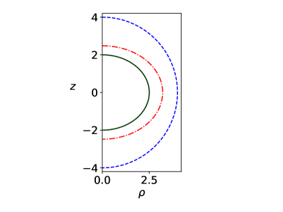
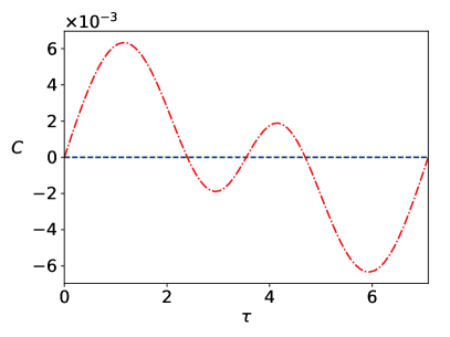
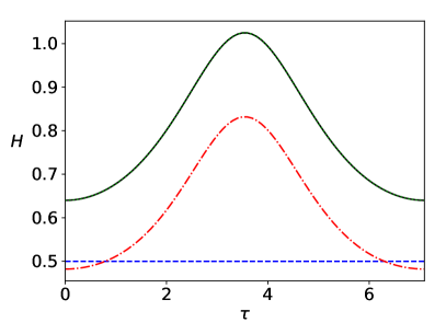
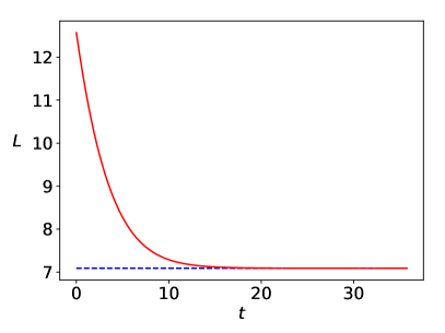
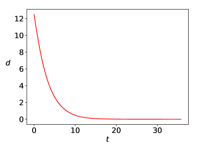
Figure 1: Flow with fixed Euclidean background metric. The initial curve is taken to be a circle in Weyl–Papapetrou (= Euclidean cylindrical) coordinates (radius $r_{0}=4$, parametrised by arclength) and the target curve an ellipse (semi-major axes $\overline{\rho}=2.5,\overline{z}=2$). Shown are the coordinate location of the curve (top panel), the embedding term $C$ and the mean curvature $H$ (middle panels) at flow times $t=0$ (dashed blue), $t=3.6$ (dash-dotted red) and $t=35.8$ (dotted green). The target curve is plotted in solid black (indistinguishable from the dotted green curve here). In the bottom panels, we plot the total curve length $L$ (with the target length $\overline{L}$ shown in dashed blue) and the Euclidean distance $d$ to the target curve (5.4) as functions of flow time $t$.

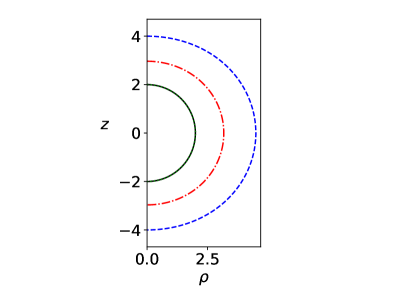
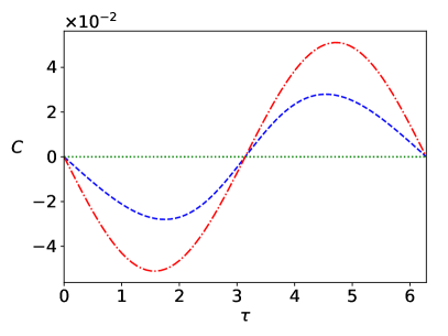
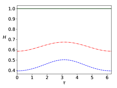
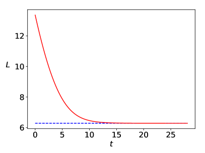
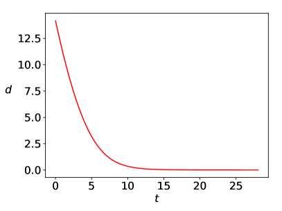
Figure 2: Flow with fixed Euclidean background metric. The initial curve is taken to be an ellipse in Weyl–Papapetrou (=Euclidean cylindrical) coordinates (semi-major axes $\rho_{0}=4.5,z_{0}=4$) which in this case is not parametrised by arclength. The target curve is a circle (radius $\overline{r}=2$). The same quantities as in Figure 1 are plotted. In the first three panels, the curves correspond to flow times $t=0$ (dashed blue), $t=2.8$ (dash-dotted red) and $t=28.1$ (dotted green), with the target solution plotted in solid black.

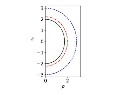
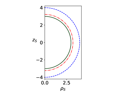
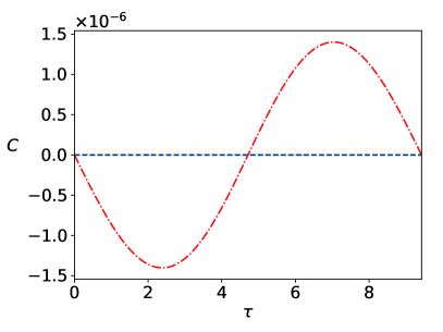
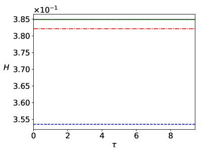
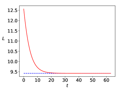
Figure 3: Flow with fixed background Schwarzschild metric ($M=1$). The initial curve is taken to be a circle in Schwarzschild coordinates (radius $r_{S,0}=4$, parametrised by arclength) and the target curve a smaller circle ($\overline{r}_{S}=3$), also in Schwarzschild coordinates. Here the top panels show the coordinate location of the curve in Weyl–Papapetrou and Schwarzschild coordinates, respectively. The remaining quantities are the same as in Figure 1. In the first four panels, the curves correspond to flow times $t=0$ (dashed blue), $t=6.3$ (dash-dotted red) and $t=63.2$ (dotted green), with the target solution plotted in solid black.

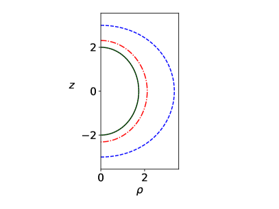
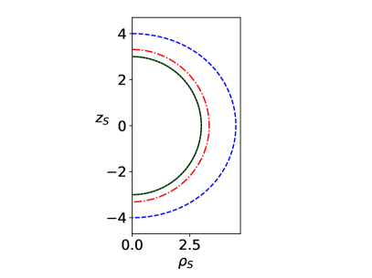
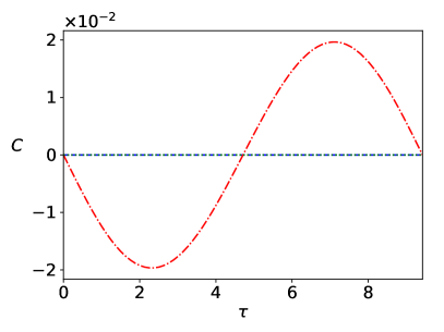
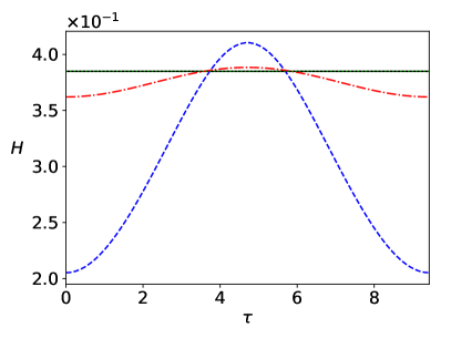
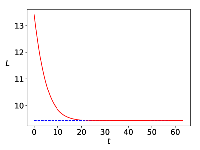
Figure 4: Flow with fixed background Schwarzschild metric ($M=1$). The initial curve is taken to be an ellipse in Schwarzschild coordinates (semi-major axes $\rho_{S,0}=4.5,z_{S,0}=4$, parametrised by arclength) and the target curve a circle ($\overline{r}_{S}=3$), also in Schwarzschild coordinates. The same quantities as in Figure 3 are plotted. In the first four panels, the curves correspond to flow times $t=0$ (dashed blue), $t=6.3$ (dash-dotted red) and $t=63.2$ (dotted green), with the target solution plotted in solid black.

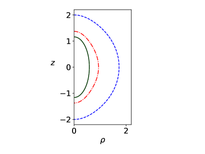
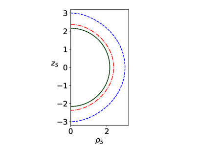
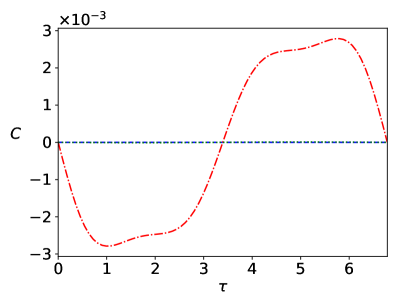
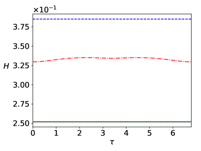
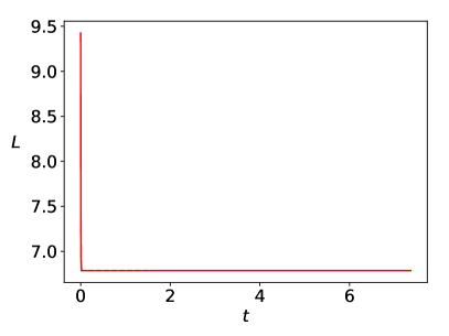
Figure 5: Flow with fixed background Schwarzschild metric ($M=1$). The initial curve is taken to be a circle in Schwarzschild coordinates (radius $r_{S,0}=3$, parametrised by arclength) and the target curve a circle close to the horizon ($\overline{r}_{S}=2.16$), also in Schwarzschild coordinates. The same quantities as in Figure 3 are plotted. In the first four panels, the curves correspond to flow times $t=0$ (dashed blue), $t=0.0041$ (dash-dotted red) and $t=7.4$ (dotted green), with the target solution plotted in solid black. The total curve length $L$ decreases rapidly to its target value on the time scale shown.

5.2 Evolving metric

In this section, we let the metric evolve along with the flow by solving the Weyl–Papapetrou equations (2.5), (2.6) for $U$ and $V$ as described in Section 4.2. The numerical resolution is taken to be $N=30$ collocation points throughout this subsection.

In order to obtain some insight into how the static metric extensions change during the flow, we compute three masses at each time step, namely the (total) ADM mass $m_{\mathrm{ADM}}$ (1.7), the (quasi-local) Hawking mass $m_{\mathrm{H}}$ (1.8), and the pseudo-Newtonian mass $m_{\mathrm{PN}}$ (1.10) of the boundary surface corresponding to the flowing curve $\Gamma_{t}=x^{a}_{t}(\tau)$ in the static metric extension corresponding to $U_{t}$ and $V_{t}$. We remind the reader that the relations between these masses were briefly discussed in Section 1.1.

As the ADM mass can easily be seen to be the leading order term in an expansion of $U$ in inverse powers of $r$,

$$U =-\frac{m_{\mathrm{ADM}}}{r}+\mathcal{O}\left(\frac{1}{r^{2}}\right),$$ (5.5)

and can thus be computed as the first expansion coefficient in the Legendre expansion (4.17) that we use to solve the Weyl–Papapetrou equations:

$$m_{\mathrm{ADM}} =a_{0}.$$ (5.6)

Combining the definition of the Hawking mass (1.8) with our expression for the mean curvature (2.14) and for the induced $2$-metric (2.9), the Hawking mass of the boundary surface corresponding to $\Gamma_{t}=x^{a}_{t}(\tau)$ is obtained as

$$\begin{split}m_{\mathrm{H}}&=\sqrt{\frac{1}{8}\int_{0}^{\overline{L}}\ell\,r\,\sin\theta\,e^{-U\circ\gamma}\,\mathrm{d}\tau}\\ &\qquad\times\left(1-\frac{1}{8}\int_{0}^{\overline{L}}H^{2}\,\ell\,r\,\sin\theta\,e^{-U\circ\gamma}\,\mathrm{d}\tau\right).\end{split}$$ (5.7)

Similarly, the pseudo-Newtonian mass (1.10) of the boundary surface corresponding to $\Gamma_{t}=x^{a}_{t}(\tau)$ can be computed to be

$$m_{\mathrm{PN}} =\frac{1}{2}\int_{0}^{\overline{L}}(r^{2}\theta^{\prime}\,U_{,r}\circ\gamma-r^{\prime}\,U_{,\theta}\circ\gamma)\sin\theta\,\mathrm{d}\tau,$$ (5.8)

where we used (2.3) and (2.9).

In the following figures, the masses are shown as functions of flow time $t$ in the bottom right panel: the ADM mass (solid blue), the Hawking mass (dashed green) and the pseudo-Newtonian mass (dash-dotted red). In many plots the curves coincide. Recall from Section 1.1 that the ADM and the pseudo-Newtonian mass must theoretically be identical, while the Hawking mass will in general be smaller than the other two masses, except on round spheres in Euclidean space and on centred round spheres in Schwarzschild, where all three notions of mass coincide.

Our numerical analysis for the coupled flow–Weyl–Papapetrou system now proceeds as follows. In this subsection, we construct Bartnik data by specifying the coordinate location of the target curve in a given background metric, as in Section 5.1. (We will consider more general Bartnik data in Section 5.3.)

In Figure 6, we choose as target curve an ellipse in Euclidean space. The initial curve is taken to be a circle in Euclidean space. Already at the initial time, the flow departs from Euclidean space because the initial (vanishing) $U$ and $V$ are replaced with the (non-trivial) solution to the Weyl–Papapetrou equations with boundary data determined by the prescribed function $\overline{\lambda}(\tau)$ according to (2.11), see also Section 3.2.1. This also implies that the initial curve is no longer parametrised by arclength once $U$ and $V$ have been updated, hence $C\neq 0$ initially. The flow does converge to the target curve and the Euclidean metric as desired. This example shows clearly how the Hawking mass can differ from the other masses; in this case it is negative, whereas the other masses are zero. It should be noted that the expressions we use for the masses are only physically meaningful as $t\to\infty$ as the curve becomes parametrised by arclength.

In Figure 7, we present a flow from a circle in Euclidean space to a (Schwarzschild coordinate) circle in Schwarzschild space ($M=1$). Figure 8 shows a similar evolution of a (Schwarzschild coordinate) circle in Schwarzschild space of mass $M=1$ to a different Schwarzschild space of mass $M=2$. In Figure 9, we let a (Schwarzschild coordinate) circle in $M=1$ Schwarzschild space flow to a circle close to the horizon ($\overline{r}_{S}=2.41$) in the same Schwarzschild system (but again notice that the coupled flow departs from this metric at intermediate times). This is the closest we could get to the horizon at $r_{S}=2$ due to the numerical problems associated with our method of solving the Laplace equation for $U$ described in Section 4.2.

A flow between different members of the Zipoy–Voorhees family is shown in Figure 10 and between different members of the Curzon–Chazy family in Figure 11. In this case, the Hawking mass can be seen to differ noticeably from the other mass functions, as was to be expected.

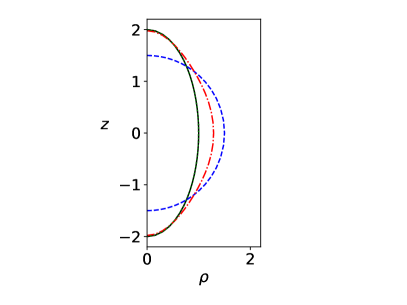
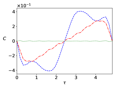
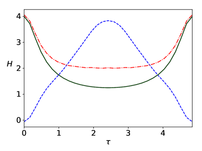
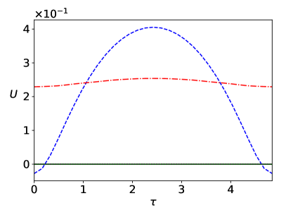
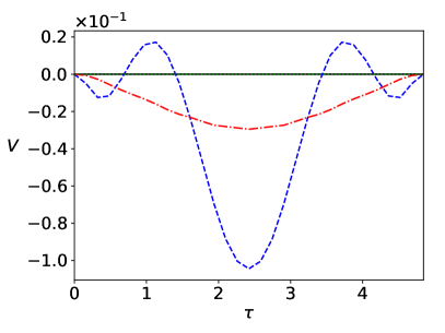
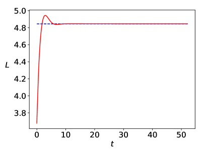
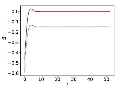
Figure 6: Flow with evolving metric. The initial curve is taken to be a circle in Euclidean space ($r_{0}=1.5$), the target curve an ellipse in Euclidean space (semi-major axes $\overline{\rho}=1,\overline{z}=2$). In addition to the quantities described in Figure 1, we also show the metric fields $U$ and $V$ along the flowing curve here. The different curves correspond to flow times $t=0$ (dashed blue), $t=0.26$ (dash-dotted red) and $t=52.1$ (dotted green), with the target solution plotted in solid black. In the bottom right panel we plot the three masses described in the main text: ADM (solid blue), Hawking (dashed green) and pseudo-Newtonian (dash-dotted red, indistinguishable from the solid blue line).

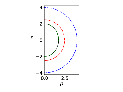
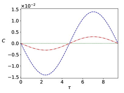
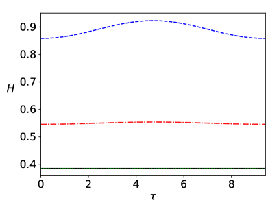
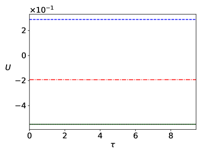
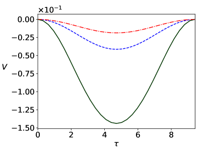
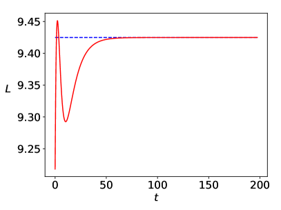
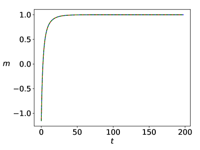
Figure 7: Flow with evolving metric. The initial curve is taken to be a circle in Euclidean space ($r_{0}=4$), the target curve a circle in Schwarzschild coordinates ($\overline{r}_{S}=3$) in Schwarzschild space of mass $M=1$. The same quantities as in Figure 6 are plotted. In the first five panels, the different curves correspond to flow times $t=0$ (dashed blue), $t=4.9$ (dash-dotted red) and $t=197.4$ (dotted green), with the target solution plotted in solid black.

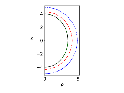
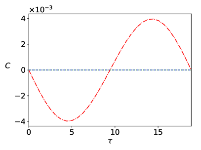
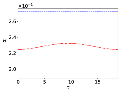
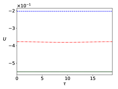
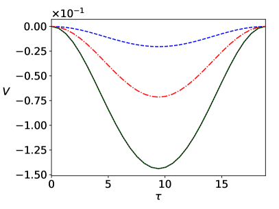
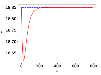
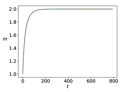
Figure 8: Flow with evolving metric. The initial curve is taken to be a circle ($r_{S,0}=6$) in $M=1$ Schwarzschild space, the target curve a circle ($\overline{r}_{S}=6$) in $M=2$ Schwarzschild space. The same quantities as in Figure 6 are plotted. In the first five panels, the different curves correspond to flow times $t=0$ (dashed blue), $t=19.7$ (dash-dotted red) and $t=789.6$ (dotted green), with the target solution plotted in solid black.

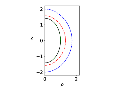
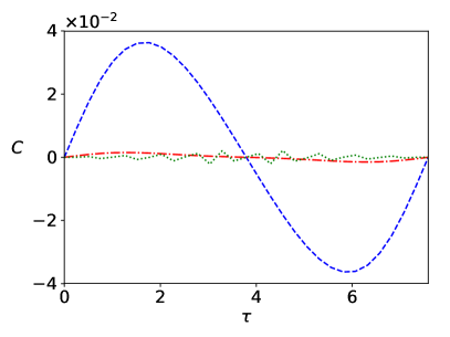
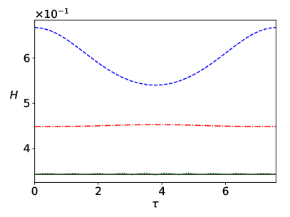
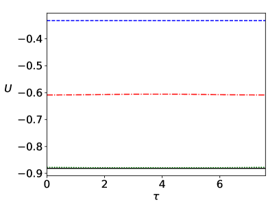
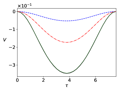
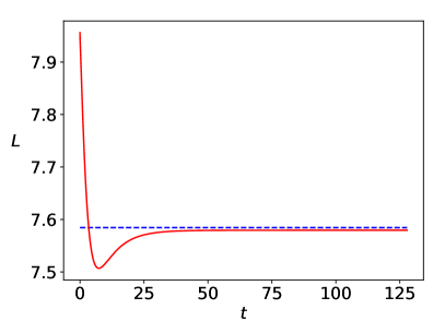
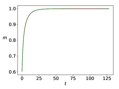
Figure 9: Flow with evolving metric. The initial curve is taken to be a (Schwarzschild coordinate) circle ($r_{S,0}=3$) in $M=1$ Schwarzschild space, the target curve a (Schwarzschild coordinate) circle close to the horizon ($\overline{r}_{S}=2.41$) in Schwarzschild space of the same mass $M=1$. The same quantities as in Figure 6 are plotted. In the first five panels, the different curves correspond to flow times $t=0$ (dashed blue), $t=3.2$ (dash-dotted red) and $t=127.8$ (dotted green), with the target solution plotted in solid black.

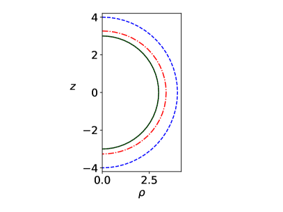
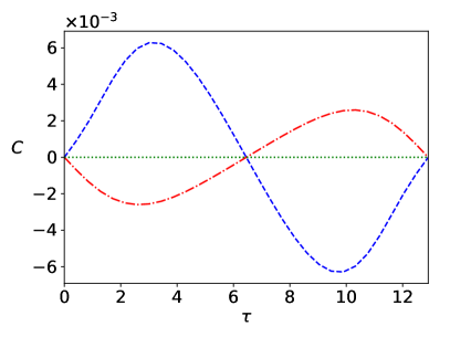
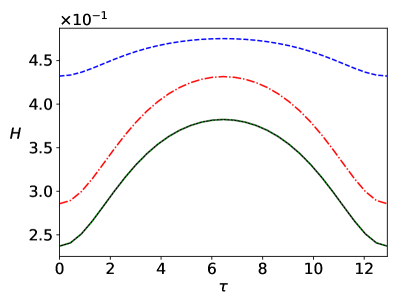
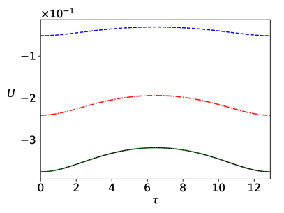
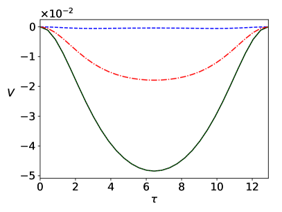
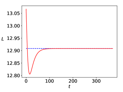
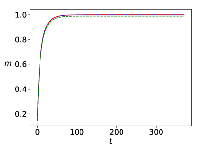
Figure 10: Flow with evolving metric. The initial curve is taken to be a Weyl–Papapetrou coordinate circle ($r_{0}=4$) in the Zipoy–Voorhees space with parameters $M=1,\delta=0.7$, the target curve a Weyl–Papapetrou coordinate circle ($\overline{r}=3$) in the Zipoy–Voorhees space with parameters $M=1,\delta=0.6$. The same quantities as in Figure 6 are plotted. In the first five panels, the different curves correspond to flow times $t=0$ (dashed blue), $t=9.3$ (dash-dotted red) and $t=370.3$ (dotted green), with the target solution plotted in solid black.

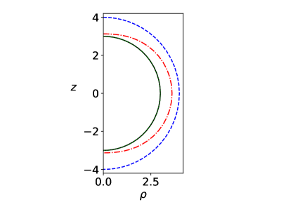
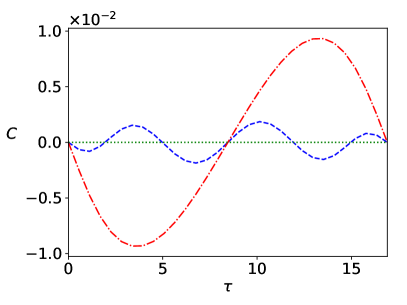
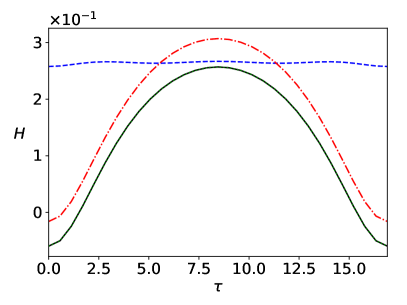
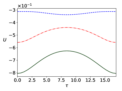
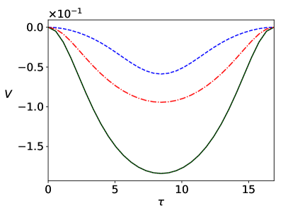
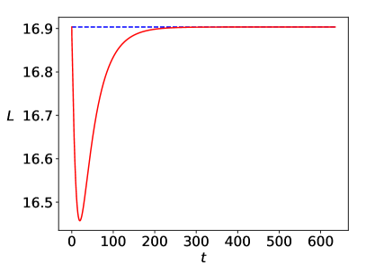
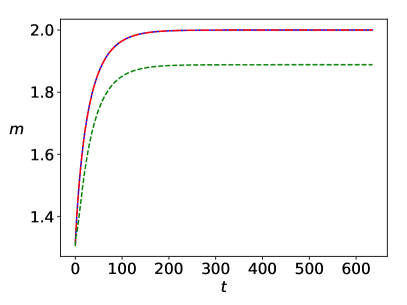
Figure 11: Flow with evolving metric. The initial curve is taken to be a Weyl–Papapetrou coordinate circle ($r_{0}=4$) in the Curzon–Chazy space of mass $M=1$, the target curve a Weyl–Papapetrou coordinate circle ($\overline{r}=3$) in the Curzon–Chazy space of mass $M=2$. The same quantities as in Figure 6 are plotted. In the first five panels, the different curves correspond to flow times $t=0$ (dashed blue), $t=15.9$ (dash-dotted red) and $t=634.9$ (dotted green), with the target solution plotted in solid black.

5.3 Perturbed Bartnik data

In the simulations presented so far, we constructed the Bartnik data from a given Weyl–Papapetrou system, and the flow correctly recovered the corresponding metric extension. To conclude this section, we now study a case where we do not know a priori which exterior metric the Bartnik data give rise to. To construct such data, we start with a Schwarzschild coordinate circle at the photon sphere $r_{S\circ}=3M$. (We use the photon sphere here since it is a geometrically distinguished round sphere where the mean curvature $H_{\circ}$ is maximal.) We compute the corresponding Killing vector norm $\overline{\lambda}_{\circ}(\tau)$ and then perturb this function:

$$\overline{\lambda}(\tau)=\overline{\lambda}_{\circ}(\tau)(1+f(\tau)),$$ (5.9)

where we choose a Gaussian profile

$$f(\tau)=A\exp\left(-\left(\frac{\tau-\tau_{0}}{\sigma}\right)\right).$$ (5.10)

We compute a new Schwarzschild coordinate radius $r_{S}$ from

$$r_{S}\mathrel{\raise 0.40903pt\hbox{\rm:}\mkern-5.2mu=}\sqrt{\frac{|\Sigma|}{4\pi}},\qquad|\Sigma|\mathrel{\raise 0.40903pt\hbox{\rm:}\mkern-5.2mu=}2\pi\int_{0}^{\overline{L}}\overline{\lambda}(\tau)\,\mathrm{d}\tau,$$ (5.11)

where $\overline{L}$ is taken from the unperturbed target curve (note that we do not know the coordinate location of the target curve corresponding to the perturbed Bartnik data in this case). We choose the mean curvature to have the constant value

$$\overline{H}(\tau)=\frac{2}{\sqrt{3}\,r_{S}},$$ (5.12)

the same functional dependence as between $H_{\circ}$ and $r_{S\circ}$.

Figure 12 demonstrates that the flow converges; we have thus constructed the static metric extension corresponding to the prescribed Bartnik data $([0,\overline{L}],\overline{\lambda},\overline{H})$. The chosen amplitude $A=0.1$ of the perturbation is the maximum value for which we were able to achieve a stable numerical evolution. We choose $M=1$ for the unperturbed target curve. The final ADM mass is $m_{\mathrm{ADM}}=1.0200$ and the final Hawking mass is $m_{\mathrm{H}}=1.0162$. This is in accordance with the generalised Penrose inequality (1.9).

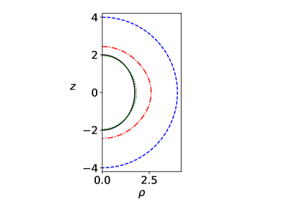
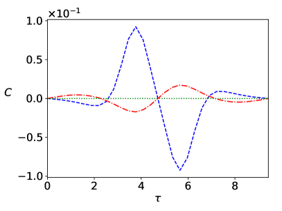
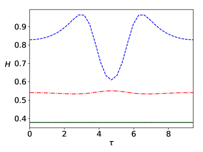
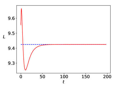
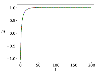
Figure 12: Flow with evolving metric. The Bartnik data are constructed from the photon sphere in $M=1$ Schwarzschild perturbed by a Gaussian profile (5.10) with $A=0.1$, $\tau_{0}=\overline{L}/2$ and $\sigma=\overline{L}/8$. The initial curve is taken to be a circle with radius $r_{S}=4$ in $M=1$ Schwarzschild. Solid black lines refer to the unperturbed data. The final ADM mass belonging to the perturbed Bartnik data is $m_{\mathrm{ADM}}=1.0200$ and the Hawking mass is $m_{\mathrm{H}}=1.0162$. In the first five panels, the different curves correspond to flow times $t=0$ (dashed blue), $t=4.9$ (dash-dotted red) and $t=197.4$ (dotted green). Solid black lines refer to the unperturbed data here.

In Figure 13, we investigate the dependence of the masses (ADM, Hawking, and pseudo-Newtonian) on the amplitude $A$ of the perturbation. All three masses appear to approach the unperturbed value continuously as $A\to 0$. The ADM mass and the pseudo-Newtonian mass are identical within numerical error, as expected from the theoretical analysis, see Section 1.1.

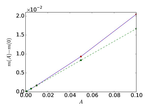
Figure 13: Dependence of the masses on the amplitude $A$ of the perturbation for the Bartnik data with Gaussian perturbation as in Figure 12. Shown are the ADM mass (solid blue), the Hawking mass (dashed green), and the pseudo-Newtonian mass (dash-dotted red, indistinguishable from the solid blue line).

6 Conclusion

In this paper, we developed a new approach to construct static metric extensions as they arise in Bartnik’s conjecture. We restricted ourselves to axisymmetry and worked with the Weyl–Papapetrou formulation of the static axisymmetric vacuum (SAV) Einstein equations. The metric extension problem becomes an elliptic free boundary value problem in this setting, which we solved numerically using a geometric flow (2.23) coupled to the Weyl–Papapetrou system of equations (2.5), (2.6). As far as we know, this is the first time static metric extensions have been constructed explicitly in general situations using numerical methods.

It should be noted that we only considered axisymmetric Bartnik data, and we only sought axisymmetric static metric extensions. Even for axisymmetric data, non-axisymmetric static metric extensions might exist. Furthermore, we restricted our attention to reflection-symmetric Bartnik data and static metric extensions. Of course, even for reflection symmetric data, non-reflection symmetric static metric extensions may exist.

In a first step, we simplified the situation by fixing the metric to some known background SAV solution to the Einstein equations and prescribing Bartnik data corresponding to a given surface within that spacetime, or rather to a given curve after performing the symmetry reduction. We showed analytically that coordinate circles in Euclidean space and in a fixed Schwarzschild background remain coordinate circles during our geometric flow and approach the desired target circles in a globally stable manner. Moreover, coordinate circles in Euclidean space are linearly stable against arbitrary perturbations. We also presented arguments in favour of short-time existence of solutions to (2.23). It would be very interesting to study short-time existence of the flow more rigorously.

Numerically, our geometric flow behaved as expected in this situation. Interestingly, in Euclidean space, the Euclidean distance (5.4) between the flowing and the target curve appeared to decrease monotonically in all cases we studied numerically. Investigating this claim analytically would be an interesting topic for future work.

Next, we studied the full elliptic free boundary value problem, which involved solving the Weyl–Papapetrou form (2.5), (2.6) of the SAV Einstein equations at each “time” step of the flow. We specified Bartnik data corresponding to given surfaces in various known SAV spacetimes, and in all cases where we obtained stable numerical evolutions, the surface and static metric extension were found correctly. We also perturbed Bartnik data corresponding to (centred) round spheres in Schwarzschild so that we did not know the corresponding metric extensions a priori, and we were able to construct static metric extensions with ADM masses up to $2\%$ larger than in the unperturbed case. The ADM mass appeared to approach the unperturbed mass continuously in the limit of vanishing amplitude of the perturbation. The Hawking mass was always observed to be smaller than or equal to the ADM mass (or, identically, the pseudo-Newtonian mass), in agreement with the generalised Penrose inequality (1.9). These results should be interesting in the light of ongoing analytical work on the case of near-round spheres in Schwarzschild in [8].

Our analysis revealed that theoretically, the flow has more stationary states than just the desired position of a curve inducing the correct Bartnik data (even in a fixed Euclidean background), although in all the simulations shown in this paper, the flow did approach the desired stationary state. Investigating if there really can be evolutions approaching one of the spurious stationary states and developing suitable work-around strategies would be an interesting topic for future research.

In all situations where we investigated this, different initial data to the coupled flow gave rise to the same asymptotic solution $(U,V)$ as $t\to\infty$. If we had found an example where this is not the case then this would disprove the uniqueness of static metric extensions for given Bartnik data. It should be interesting to investigate this uniqueness question in more extreme situations.

We encountered numerical instabilities e.g. when we specified Bartnik data corresponding to a surface too close to the horizon in Schwarzschild or when the flowing curves became too strongly deformed (e.g. ellipses with large eccentricity). Sometimes, it was possible to cure these instabilities by adapting the parameter $\kappa$ in (2.23) or by making the time steps sufficiently small. Another source of numerical instability was associated with our method of solving the Poisson equation (2.5) for the metric field $U$ described in Section 4.2 and arose when the radius of the flowing curve became too small, $r\lesssim 1$ in Weyl–Papapetrou coordinates. It was possible to somewhat alleviate this problem by the least squares method (also described in Section 4.2). More work is needed to obtain stable simulations in more extreme situations.

From an analytical perspective, it would be very interesting indeed to rigorously analyse the full coupled elliptic system with flowing boundary, equations (2.5), (2.6) and (2.23), and to thereby obtain theoretical results about existence of solutions to Bartnik’s static metric extension conjecture in Weyl–Papapetrou form.

References

- [1] {barticle}[author] \bauthor\bsnmAnderson, \bfnmM.\binitsM. (\byear2015). \btitleLocal existence and uniqueness for exterior static vacuum Einstein metrics. \bjournalProceedings of the American Mathematical Society \bvolume143 \bpages3091–3096. \endbibitem
- [2] {barticle}[author] \bauthor\bsnmAnderson, \bfnmMichael T\binitsM. T. and \bauthor\bsnmKhuri, \bfnmMarcus A\binitsM. A. (\byear2013). \btitleOn the Bartnik extension problem for the static vacuum Einstein equations. \bjournalClassical and Quantum Gravity \bvolume30 \bpages125005. \bdoi10.1088/0264-9381/30/12/125005 \endbibitem
- [3] {barticle}[author] \bauthor\bsnmArnowitt, \bfnmR.\binitsR., \bauthor\bsnmDeser, \bfnmS.\binitsS. and \bauthor\bsnmMisner, \bfnmCh.\binitsC. (\byear1961). \btitleCoordinate Invariance and Energy Expressions in General Relativity. \bjournalPhys. Rev. \bvolume122 \bpages997–1006. \endbibitem
- [4] {barticle}[author] \bauthor\bsnmBartnik, \bfnmRobert\binitsR. (\byear1986). \btitleThe Mass of an Asymptotically Flat Manifold. \bjournalCommunications on Pure and Applied Mathematics \bvolume39 \bpages661–693. \bdoi10.1002/cpa.3160390505 \endbibitem
- [5] {barticle}[author] \bauthor\bsnmBartnik, \bfnmR.\binitsR. (\byear1989). \btitleNew Definition of Quasilocal Mass. \bjournalPhys. Rev. Lett. \bvolume62 \bpages2346–2348. \endbibitem
- [6] {bbook}[author] \bauthor\bsnmBoyd, \bfnmJ. B.\binitsJ. B. (\byear2001). \btitleChebyshev and Fourier Spectral Methods, \bedition2nd edn. ed. \bpublisherDover. \endbibitem
- [7] {bphdthesis}[author] \bauthor\bsnmCederbaum, \bfnmC.\binitsC. (\byear2011). \btitleThe Newtonian Limit of Geometrostatics. \btypePhD thesis, \bpublisherFreie Universität Berlin. \endbibitem
- [8] {bmisc}[author] \bauthor\bsnmCederbaum, \bfnmC.\binitsC. and \bauthor\bsnmEscobar Diaz, \bfnmL.\binitsL. \bnoteWork in progress. \endbibitem
- [9] {barticle}[author] \bauthor\bsnmChrúsciel, \bfnmPiotr T.\binitsP. T. (\byear1988). \btitleOn the invariant mass conjecture in general relativity. \bjournalCommunications in Mathematical Physics \bvolume120 \bpages233–248. \endbibitem
- [10] {barticle}[author] \bauthor\bsnmCourant, \bfnmR.\binitsR., \bauthor\bsnmFriedrichs, \bfnmK.\binitsK. and \bauthor\bsnmLewy, \bfnmH.\binitsH. (\byear1928). \btitleÜber die partiellen Differenzengleichungen der mathematischen Physik. \bjournalMath. Ann. \bvolume100 \bpages32–74. \endbibitem
- [11] {bphdthesis}[author] \bauthor\bsnmDittberner, \bfnmF.\binitsF. (\byear2017). \btitleConstrained Curve Flows. \btypePhD thesis, \bpublisherFreie Universität Berlin. \endbibitem
- [12] {bbook}[author] \bauthor\bsnmFornberg, \bfnmB.\binitsB. (\byear1996). \btitleA Practical Guide to Pseudospectral Methods. \bseriesCambridge Monographs on Applied and Computational Mathematics. \bpublisherCambridge University Press. \endbibitem
- [13] {bincollection}[author] \bauthor\bsnmGage, \bfnmM. E.\binitsM. E. (\byear1986). \btitleOn an area preserving evolution equation for plane curves. In \bbooktitleNonlinear Problems in Geometry, (\beditor\bfnmD. M.\binitsD. M. \bsnmDeTurck, ed.). \bseriesContemporary Mathematics \bvolume51 \bpages51–62. \endbibitem
- [14] {bbook}[author] \bauthor\bsnmGriffiths, \bfnmJ. B.\binitsJ. B. and \bauthor\bsnmPodolský, \bfnmJ.\binitsJ. (\byear2012). \btitleExact space-times in Einstein’s general relativity. \bseriesCambridge Monographs on Mathematical Physics. \bpublisherCambridge University Press. \endbibitem
- [15] {barticle}[author] \bauthor\bsnmHawking, \bfnmStephen W.\binitsS. W. (\byear1968). \btitleGravitational radiation in an expanding universe. \bjournalJ. Math. Phys. \bvolume9 \bpages598–604. \bdoi10.1063/1.1664615 \endbibitem
- [16] {barticle}[author] \bauthor\bsnmHuisken, \bfnmG.\binitsG. (\byear1987). \btitleThe volume preserving mean curvature flow. \bjournalJ. Reine Angew. Math. \bvolume382 \bpages35–48. \endbibitem
- [17] {binproceedings}[author] \bauthor\bsnmHuisken, \bfnmGerhard\binitsG. and \bauthor\bsnmIlmanen, \bfnmTom\binitsT. (\byear2002). \btitleEnergy Inequalities for Isolated Systems and Hypersurfaces Moving by their Curvature. In \bbooktitleProceedings of the 16th International Conference on General Relativity and Gravitation (\beditor\bfnmNigel T.\binitsN. T. \bsnmBishop and \beditor\bfnmSunil D.\binitsS. D. \bsnmMaharaj, eds.) \bpages162–173. \bpublisherWorld Scientific. \endbibitem
- [18] {barticle}[author] \bauthor\bsnmJauregui, \bfnmJeffrey L.\binitsJ. L. (\byear2013). \btitleFill-ins of nonnegative scalar curvature, static metrics, and quasi-local mass. \bjournalPacific J. Math. \bvolume261 \bpages417–444. \endbibitem
- [19] {barticle}[author] \bauthor\bsnmKomar, \bfnmArthur\binitsA. (\byear1963). \btitlePositive-Definite Energy Density and Global Consequences for General Relativity. \bjournalPhysical Review \bvolume129 \bpages1873–1876. \endbibitem
- [20] {barticle}[author] \bauthor\bsnmMiao, \bfnmP.\binitsP. (\byear2003). \btitleOn the existence of static metric extensions in general relativity. \bjournalCommun. Math. Phys. \bvolume241 \bpages24–46. \endbibitem
- [21] {barticle}[author] \bauthor\bsnmPapapetrou, \bfnmA.\binitsA. (\byear1948). \btitleA static solution of the equations of the gravitational field for an arbitrary charge-distribution. \bjournalProc. R. Irish Acad. A \bvolume52. \endbibitem
- [22] {bphdthesis}[author] \bauthor\bsnmPihan, \bfnmD. M.\binitsD. M. (\byear1998). \btitleA length preserving geometric heat flow for curves. \btypePhD thesis, \bpublisherUniversity of Melbourne. \endbibitem
- [23] {bmastersthesis}[author] \bauthor\bsnmPiubello, \bfnmA.\binitsA. (\byear2017). \btitleOn Existence of Static Metric Extensions à la Miao. \btypeMaster’s thesis, \bpublisherUniversity of Tübingen. \endbibitem
- [24] {barticle}[author] \bauthor\bsnmSchwarzschild, \bfnmK.\binitsK. (\byear1916). \btitleÜber das Gravitationsfeld eines Massenpunktes nach der Einsteinschen Theorie. \bjournalSitzungsberichte der Königlich Preußischen Akademie der Wissenschaften \bvolume7 \bpages189–196. \endbibitem
- [25] {bbook}[author] \bauthor\bsnmTaylor, \bfnmM. E.\binitsM. E. (\byear2011). \btitlePartial Differential Equations III. \bseriesApplied Mathematical Sciences \bvolume117. \bpublisherSpringer, \baddressNew York. \endbibitem
- [26] {barticle}[author] \bauthor\bsnmWeyl, \bfnmH.\binitsH. (\byear1917). \btitleZur Gravitationstheorie. \bjournalAnn. Physik \bvolume54 \bpages117–145. \endbibitem