Evidence for Late-stage Eruptive Mass-loss in the Progenitor to SN2018gep, a Broad-lined Ic Supernova:
Pre-explosion Emission and a Rapidly Rising Luminous Transient

Abstract

We present detailed observations of ZTF18abukavn (SN2018gep), discovered in high-cadence data from the Zwicky Transient Facility as a rapidly rising ($1.4\pm 0.1$ mag/hr) and luminous ($M_{g,\mathrm{peak}}=-20$ mag) transient. It is spectroscopically classified as a broad-lined stripped-envelope supernova (Ic-BL SN). The high peak luminosity ($\mbox{$L_{\mathrm{bol}}$}\gtrsim 3\times 10^{44}\,\mbox{$\rm erg$}\,\mbox{$\rm s^{-1}$}$), the short rise time ($\mbox{$t_{\rm rise}$}=3\,\mbox{$\rm day$}$ in $g$-band), and the blue colors at peak ($g-r\sim-0.4$) all resemble the high-redshift Ic-BL iPTF16asu, as well as several other unclassified fast transients. The early discovery of SN2018gep (within an hour of shock breakout) enabled an intensive spectroscopic campaign, including the highest-temperature ($\mbox{$T_{\rm eff}$}\gtrsim 40,000\mbox{$\rm K$}$) spectra of a stripped-envelope SN. A retrospective search revealed luminous ($M_{g}\sim M_{r}\approx-14\,$mag) emission in the days to weeks before explosion, the first definitive detection of precursor emission for a Ic-BL. We find a limit on the isotropic gamma-ray energy release $E_{\mathrm{\gamma,iso}}<4.9\times 10^{48}\,\mbox{$\rm erg$}$, a limit on X-ray emission $L_{\mathrm{X}}<10^{40}\,\mbox{$\rm erg$}\,\mbox{$\rm s^{-1}$}$, and a limit on radio emission $\nu L_{\nu}\lesssim 10^{37}\,\mbox{$\rm erg$}\,\mbox{$\rm s^{-1}$}$. Taken together, we find that the early ($<10\,\mbox{$\rm day$}$) data are best explained by shock breakout in a massive shell of dense circumstellar material (0.02 $M_{\odot}$) at large radii ($3\times 10^{14}\,\mbox{$\rm cm$}$) that was ejected in eruptive pre-explosion mass-loss episodes. The late-time ($>10\,\mbox{$\rm day$}$) light curve requires an additional energy source, which could be the radioactive decay of Ni-56.

astro-ph/1904.11009

1 Introduction

Recent discoveries by optical time-domain surveys challenge our understanding of how energy is deposited and transported in stellar explosions (Kasen, 2017). For example, over 50 transients have been discovered with rise times and peak luminosities too rapid and too high, respectively, to be explained by radioactive decay (Poznanski et al., 2010; Drout et al., 2014; Shivvers et al., 2016; Tanaka et al., 2016; Arcavi et al., 2016; Rest et al., 2018; Pursiainen et al., 2018). Possible powering mechanisms include interaction with extended circumstellar material (CSM; Chevalier & Irwin 2011), and energy injection from a long-lived central engine (Kasen & Bildsten, 2010; Woosley, 2010; Kasen et al., 2016). These models have been difficult to test because the majority of fast-luminous transients have been discovered post facto and located at cosmological distances ($z\sim 0.1$).

The discovery of iPTF16asu (Whitesides et al., 2017; Wang et al., 2019) in the intermediate Palomar Transient Factory (iPTF; Law et al. 2009) showed that at least some of these fast-luminous transients are energetic ($10^{52}\,\mbox{$\rm erg$}$) high-velocity (“broad-lined”; $v\gtrsim 20,000\,\mbox{$\rm km$}\,\mbox{$\rm s^{-1}$}$) stripped-envelope (Ic) supernovae (Ic-BL SNe). The light curve of iPTF16asu was unusual among Ic-BL SNe in being inconsistent with $\rm{}^{56}Ni$-decay (Cano, 2013; Taddia et al., 2019). Suggested power sources include energy injection by a magnetar, ejecta-CSM interaction, cooling-envelope emission, and an engine-driven explosion similar to low-luminosity gamma-ray bursts — or some combination thereof. Unfortunately, the high redshift ($z=0.187$) precluded a definitive conclusion.

Today, optical surveys such as ATLAS (Tonry et al., 2018) and the Zwicky Transient Facility (ZTF; Bellm et al. 2019a; Graham et al. 2019) have the areal coverage to discover rare transients nearby, as well as the cadence to discover transients when they are young ($<1\,\mbox{$\rm day$}$). For example, the recent discovery of AT2018cow at 60 $\rm Mpc$ (Smartt et al., 2018; Prentice et al., 2018) represented an unprecedented opportunity to study a fast-luminous optical transient up close, in detail, and in real-time. Despite an intense multiwavelength observing campaign, the nature of AT2018cow remains unknown – possibilities include an engine-powered stellar explosion (Prentice et al., 2018; Perley et al., 2019a; Margutti et al., 2019; Ho et al., 2019), the tidal disruption of a white dwarf by an intermediate-mass black hole (Kuin et al., 2019; Perley et al., 2019a), and an electron capture SN (Lyutikov, & Toonen, 2019). Regardless of the origin, it is clear that the explosion took place within dense material (Perley et al., 2019a; Margutti et al., 2019; Ho et al., 2019) confined to $\lesssim 10^{16}\,\mbox{$\rm cm$}$ (Ho et al., 2019).

Here we present SN2018gep, discovered as a rapidly rising ($1.4\pm 0.1$ $\rm mag$ $\rm hr^{-1}$) and luminous ($M_{g,\mathrm{peak}}=-20$) transient in high-cadence data from ZTF (Ho et al., 2018a). The high inferred velocities ($>20,000\,\mbox{$\rm km$}\,\mbox{$\rm s^{-1}$}$), the spectroscopic evolution from a blue continuum to a Ic-BL SN (Costantin et al., 2018), the rapid rise ($\mbox{$t_{\rm rise}$}=3\,\mbox{$\rm day$}$ in $g$-band) to high peak luminosity ($\mbox{$L_{\mathrm{bol}}$}\gtrsim 3\times 10^{44}\,\mbox{$\rm erg$}\,\mbox{$\rm s^{-1}$}$) all suggest that SN2018gep is a low-redshift ($z=0.03154$) analog to iPTF16asu. The early discovery enabled an intensive follow-up campaign within the first day of the explosion, including the highest-temperature ($\mbox{$T_{\rm eff}$}\gtrsim 40,000\,\mbox{$\rm K$}$) spectra of a stripped-envelope SN to-date. A retrospective search in ZTF data revealed the first definitive detection of pre-explosion activity in a Ic-BL.

The structure of the paper is as follows. We present our radio through X-ray data in Section 2. In Section 3 we outline basic properties of the explosion and its host galaxy. In Section 4 we attribute the power source for the light curve to shock breakout in extended CSM. In Section 5 we compare SN2018gep to unidentified fast-luminous transients at high redshift. Finally, in Section 6 we summarize our findings and look to the future. Throughout the paper, absolute times are reported in UTC and relative times are reported with respect to $t_{0}$, which is defined in Section 2.1. We assume a standard $\Lambda$CDM cosmology (Planck Collaboration, 2016).

2 Observations

2.1 Zwicky Transient Facility Discovery

ZTF observing time is divided between several different surveys, conducted using a custom mosaic camera (Dekany et al., 2016) on the 48-inch Samuel Oschin Telescope (P48) at Palomar Observatory. See Bellm et al. (2019a) for an overview of the observing system, Bellm et al. (2019) for a description of the surveys and scheduler, and Masci et al. (2019) for details of the image processing system.

Every 5-$\sigma$ point-source detection is saved as an “alert.” Alerts are distributed in avro format (Patterson et al., 2019) and can be filtered based on a machine learning-based real-bogus metric (Mahabal et al., 2019; Duev et al., 2019), light-curve properties, and host characteristics (including a star-galaxy classifier; Tachibana, & Miller (2018)). The ZTF collaboration uses a web-based system called the GROWTH marshal (Kasliwal et al., 2019) to identify and keep track of transients of interest.

ZTF18abukavn was discovered in an image obtained at 2018-09-09 03:55:18 (start of exposure) as part of the ZTF extragalactic high-cadence partnership survey, which covers 1725 $\rm deg^{2}$ in six visits (3$g$, 3$r$) per night (Bellm et al., 2019). The discovery magnitude was $r=20.5\pm 0.3\,\mbox{$\rm mag$}$, and the source position was measured to be $\alpha=16^{\mathrm{h}}43^{\mathrm{m}}48.22^{\mathrm{s}}$, $\delta=+41^{\mathrm{d}}02^{\mathrm{m}}43.4^{\mathrm{s}}$ (J2000), coincident with a compact galaxy (Figure 1) at $z=\mbox{$0.03154$}$ or $d\approx\mbox{$143$}\,\mbox{$\rm Mpc$}$. As described in Section 2.3, the redshift was unknown at the time of discovery; we measured it from narrow galaxy emission lines in our follow-up spectra. The host redshift along with key observational properties of the transient are listed in Table 1.

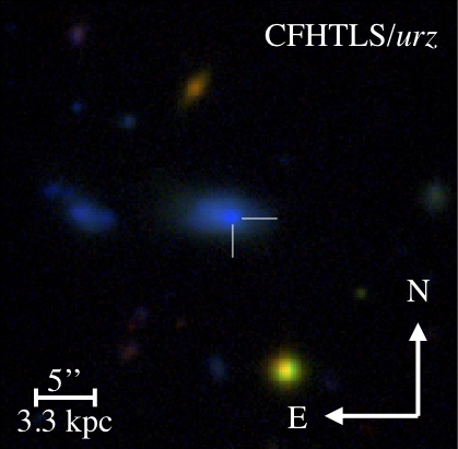
Figure 1: The position of SN2018gep (white crosshairs) in its host galaxy. Images from the Canada-France-Hawaii Telescope Legacy Survey (2004–2012), combined using the prescription in Lupton et al. (2004).

Table 1: Key observational properties of SN2018gep and its host galaxy

Parameter	Value	Notes
$z$	$0.03154$	From narrow host emission lines
$L_{\rm peak}$	$\gtrsim 3\times 10^{43}\,\mbox{$\rm erg$}$	Peak UVOIR bolometric luminosity
$t_{\rm rise}$	0.5–3 $\rm day$	Time from $t_{0}$ to $L_{\rm peak}$
$E_{\mathrm{rad}}$	$10^{50}\,\mbox{$\rm erg$}$	UVOIR output, $\Delta t=0.5$–40 $\rm day$
$M_{r,\mathrm{prog}}$	$-15$	Peak luminosity of pre-explosion emission
$E_{\mathrm{\gamma,iso}}$	$<4.9\times 10^{48}$ erg	Limit on prompt gamma-ray emission from Fermi/GBM
$L_{X}$	$<2.5\times 10^{41}\,\mbox{$\rm erg$}\,\mbox{$\rm s^{-1}$}$	X-ray upper limit from Swift/XRT at $\Delta t=0.4$–14 $\rm day$
	$<10^{40}\,\mbox{$\rm erg$}\,\mbox{$\rm s^{-1}$}$	X-ray upper limit from Chandra at $\Delta t=15$ and $\Delta t=70\,\mbox{$\rm day$}$
$\nu L_{\nu}$	$\approx 10^{37}\,\mbox{$\rm erg$}\,\mbox{$\rm s^{-1}$}$	9 $\rm GHz$ radio luminosity from VLA at $\Delta t=5$ and $\Delta t=16$
$M_{\mathrm{*,host}}$	$1.3\times 10^{8}\,M_{\odot}$	Host stellar mass
SFRhost	0.12 $M_{\odot}$ $\rm yr^{-1}$	Host star-formation rate
Host metallicity	1/5 solar	Oxygen abundance on O3N2 scale

As shown in Figure 2, the source brightened by over two magnitudes within the first three hours. These early detections passed a filter written in the GROWTH marshal that was designed to find young SNe. We announced the discovery and fast rise via the Astronomer’s Telegram (Ho et al., 2018a), and reported the object to the IAU Transient Server (TNS), where it received the designation SN2018gep.

We triggered ultraviolet (UV) and optical observations with the UV/Optical Telescope (UVOT; Roming et al. 2005) aboard the Neil Gehrels Swift Observatory (Gehrels et al., 2004), and observations began 10.2 hours after the ZTF discovery (Schulze et al., 2018a). A search of IceCube data found no temporally coincident high-energy neutrinos (Blaufuss, 2018).

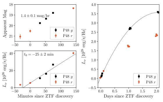
Figure 2: The rapid rise in the first few minutes and first few days after the ZTF discovery of SN2018gep. We also show an $r$-band point from prior to discovery that was found in retrospect by lowering the detection threshold from 5-$\sigma$ to 3-$\sigma$. Top left: the rise in magnitudes gives an almost unprecedented rate of $1.4\pm 0.1$ $\rm mag$ $\rm hr^{-1}$. Bottom left: the rise in flux space together with the quadratic fit and definition of $t_{0}$. Right: the rise in flux space showing the quadratic fit.

Over the first two days, the source brightened by two additional magnitudes. A linear fit to the early $g$-band photometry gives a rise of $1.4\pm 0.1$ $\rm mag$ $\rm hr^{-1}$. This rise rate is second only to the IIb SN 16gkg (Bersten et al., 2018) but several orders of magnitude more luminous at discovery ($M_{g,\mathrm{disc}}\approx-17\,\mbox{$\rm mag$}$).

To establish a reference epoch, we fit a second-order polynomial to the first three days of the $g$-band light curve in flux space, and define $t_{0}$ as the time at which the flux is zero. This gives $t_{0}$ as being $25\pm 2$ minutes prior to the first detection, or $t_{0}\approx$ UTC 2018-09-09 03:30. The physical interpretation of $t_{0}$ is not straightforward, since the light curve flattens out at early times (see Figures 2 and 3). We proceed using $t_{0}$ as a reference epoch but caution against assigning it physical meaning.

2.2 Photometry

From $\Delta t\approx 1\,\mbox{$\rm day$}$ to $\Delta t\approx 60\,\mbox{$\rm day$}$, we conducted a photometric follow-up campaign at UV and optical wavelengths using Swift/UVOT, the Spectral Energy Distribution Machine (SEDM; Blagorodnova et al. 2018) mounted on the automated 60-inch telescope at Palomar (P60; Cenko et al. 2006), the optical imager (IO:O) on the Liverpool Telescope (LT; Steele et al. 2004), and the Lulin 1-m Telescope (LOT).

Basic reductions for the LT IO:O imaging were performed by the LT pipeline. Digital image subtraction and photometry for the SEDM, LT and LOT imaging was performed using the Fremling Automated Pipeline (FPipe; Fremling et al. 2016). Fpipe performs calibration and host subtraction against Sloan Digital Sky Survey reference images and catalogs (SDSS; Ahn et al. 2014). SEDM spectra were reduced using pysedm (Rigault et al., 2019).

The UVOT data were retrieved from the NASA Swift Data Archive and reduced using standard software distributed with HEAsoft version 6.19. Photometry was measured using uvotmaghist with a $3^{\prime\prime}$ circular aperture. To remove the host contribution, we obtained a final epoch in all broad-band filters on 18 October 2018 and built a host template using uvotimsum and uvotsource with the same aperture used for the transient.

Figure 3 shows the full set of light curves, with a cross denoting the peak of the $r$-band light curve for reference. The position of the cross is simply the time and magnitude of our brightest $r$-band measurement, which is a good estimate given our cadence. The photometry is listed in Table 5 in Appendix A. Note that despite the steep SED at early times, the K-correction is minimal. We estimate that the effect is roughly 0.03 mag, which is well within our uncertainties. In Figure 4 we compare the rise time and peak absolute magnitude to other rapidly evolving transients from the literature.

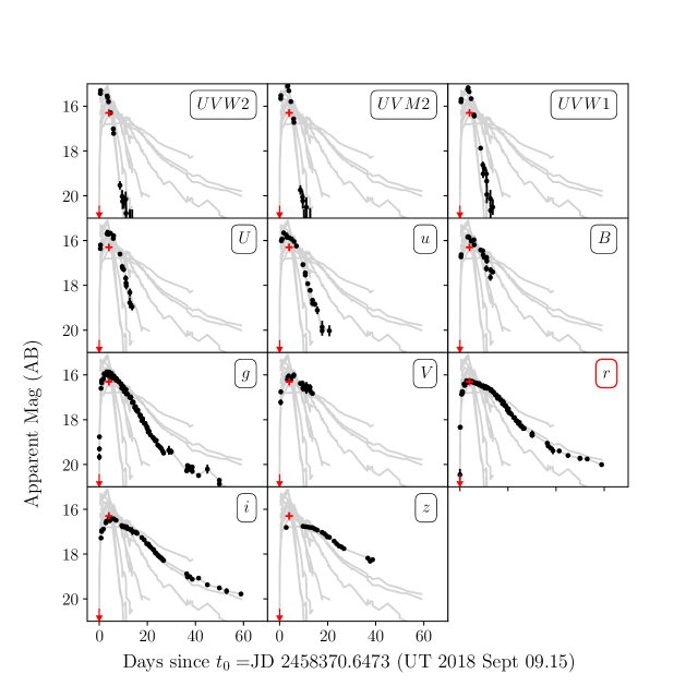
Figure 3: UV and optical light curves from Swift and ground-based facilities. The arrow marks the last non-detection, which was in $r$-band. The red cross marks the peak of the $r$-band light curve, which is 16.3 $\rm mag$ at $\Delta t=4\,\mbox{$\rm day$}$. The full set of light curves are shown as grey lines in the background, and each panel highlights an individual filter in black. We correct for Galactic extinction using the attenuation curve from Fitzpatrick (1999) and $E_{B-V}=A_{V}/R_{V}=0.01$ for $R_{V}=3.1$ and $A_{V}=0.029$ (Schlafly & Finkbeiner, 2011).

Figure 4: The rise time and peak absolute magnitude of SN2018gep, iPTF16asu (a high-redshift analog), and unclassified fast-luminous transients from Drout et al. (2014), Arcavi et al. (2016), Rest et al. (2018), and Perley et al. (2019a). When possible, we report measurements in rest-frame $g$-band, and define “rise time” as time from half-max to max. For iPTF16asu, we use the quadratic fit to the early $g$-band light curve from Whitesides et al. (2017) as well as their reported peak magnitude, but caution that this is rest-frame $r$-band. For KSN2015K, there are only observations in the Kepler white filter (Rest et al., 2018).

2.3 Spectroscopy

The first spectrum was taken 0.7 $\rm day$ after discovery by the Spectrograph for the Rapid Acquisition of Transients (SPRAT; Piascik et al. 2014) on the Liverpool Telescope (LT). The spectrum showed a blue continuum with narrow galaxy emission lines, establishing this as a luminous transient ($M_{\mathrm{g,peak}}=-19.7$). Twenty-three optical spectra were obtained from $\Delta t=0.7$–$61.1$ $\rm day$, using SPRAT, the Andalusia Faint Object Spectrograph and Camera (ALFOSC) on the Nordic Optical Telescope (NOT), the Double Spectrograph (DBSP; Oke & Gunn 1982) on the 200-inch Hale telescope at Palomar Observatory, the Low Resolution Imaging Spectrometer (LRIS; Oke et al. 1995) on the Keck I 10-m telescope, and the Xinglong 2.16-m telescope (XLT+BFOSC) of NAOC, China (Wang et al., 2018). As discussed in Section 3.2, the early $\Delta t<5\,\mbox{$\rm day$}$ spectra show broad absorption features that evolve redward with time, which we attribute to carbon and oxygen. By $\Delta t\sim 8\,\mbox{$\rm day$}$, the spectrum resembles a stripped-envelope SN, and the usual broad features of a Ic-BL emerge (Costantin et al., 2018).

We use the automated LT pipeline reduction and extraction for the LT spectra. LRIS spectra were reduced and extracted using Lpipe (Perley, 2019). The NOT spectrum was obtained at parallactic angle using a $1^{\prime\prime}$ slit, and was reduced in a standard way, including wavelength calibration against an arc lamp, and flux calibration using a spectrophotometric standard star. The XLT+BFOSC spectra were reduced using the standard IRAF routines, including corrections for bias, flat field, and removal of cosmic rays. The Fe/Ar and Fe/Ne arc lamp spectra obtained during the observation night are used to calibrate the wavelength of the spectra, and the standard stars observed on the same night at similar airmasses as the supernova were used to calibrate the flux of spectra. The spectra were further corrected for continuum atmospheric extinction during flux calibration, using mean extinction curves obtained at Xinglong Observatory. Furthermore, telluric lines were removed from the data.

Swift obtained three UV-grism spectra between 2018-09-15 3:29 and 6:58 UTC ($\Delta t\approx 6.4\,\mbox{$\rm day$}$) for a total exposure time of 3918 s. The data were processed using the calibration and software described by Kuin et al. (2015). During the observation, the source spectrum was centered on the detector, which is the default location for Swift/UVOT observations. Because of this, there is second-order contamination from a nearby star, which was reduced by using a narrow extraction width ($1.3^{\prime\prime}$ instead of $2.5^{\prime\prime}$). The contamination renders the spectrum unreliable at wavelengths longer than 4100 Å, but is negligible in the range 2850–4100 Ådue to absorption from the ISM. Below 2200 Å, the spectrum overlaps with the spectrum from another star in the field of view.

The resulting spectrum (Figure 5) shows a single broad feature between 2200 Å and 3000 Å (rest frame). One possibility is that this is a blend of the UV features seen in SLSNe. Line identifications for these features vary in the SLSN literature, but are typically blends of Ti III, Si III, C II, C III, and Mg II (Quimby et al., 2011; Howell et al., 2013; Mazzali et al., 2016; Yan et al., 2017).

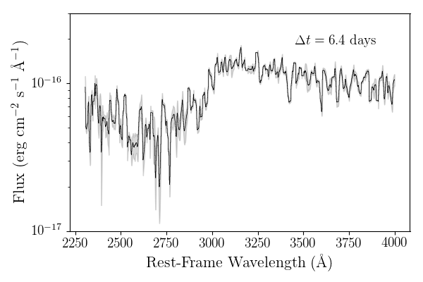
Figure 5: Swift/UVOT grism spectrum shifted to the rest frame. Black line shows the data binned such that each bin size is 10 Å. Light grey represents 1-$\sigma$ uncertainties after binning. The spectrum has been scaled to match the UVOT $u$-band flux at this epoch (integrated from 3000 Å to 3900 Å), which was determined by interpolating the Swift $u$-band light curve.

The spectral log and a figure showing all the spectra are presented in Appendix B. In Section 3.2 we compare the early spectra to spectra at similar epochs in the literature. We model one of the early spectra, which shows a “W” feature that has been seen in superluminous supernovae (SLSNe), to measure the density, density profile, and element composition of the ejecta. From the Ic-BL spectra, we measure the velocity evolution of the photosphere.

2.4 Search for pre-discovery emission

The nominal ZTF pipeline only generates detections above a 5-$\sigma$ threshold. To extend the light curve further back in time, we performed forced photometry at the position of SN2018gep on single-epoch difference images from the IPAC ZTF difference imaging pipeline. The ZTF forced photometry PSF-fitting code will be described in detail in a separate paper (Yao, Y. et al. in preparation). As shown in Figure 2, forced photometry uncovered an earlier 3-$\sigma$ $r$-band detection.

Next, we searched for even fainter detections by constructing deeper reference images than those used by the nominal pipeline, and subtracting them from 1-to-3 day stacks of ZTF science images. The reference images were generated by performing an inverse-variance weighted coaddition of 298 $R$-band and 69 $g$-band images from PTF/iPTF taken between 2009 and 2016 using the CLIPPED combine strategy in SWarp (Bertin, 2010; Gruen et al., 2014). PTF/iPTF images were used instead of ZTF images to build references as they were obtained years prior to the transient, and thus less likely to contain any transient flux. No cross-instrument corrections were applied to the references prior to subtraction. Pronounced regions of negative flux on the PTF/iPTF references caused by crosstalk from bright stars were masked out manually.

We stacked ZTF science images obtained between 2018 Feb 22 and 2018 Aug 31 in a rolling window (segregated by filter) with a width of 3 days and a period of 1 day, also using the CLIPPED technique in SWarp. Images taken between 2018 Sep 01 and $t_{0}$ were stacked in a window with a width of 1 day and a period of 1 day. Subtractions were obtained using the HOTPANTS (Becker, 2015) implementation of the Alard, & Lupton (1998) PSF matching algorithm. Many of the ZTF science images during this period were obtained under exceptional conditions, and the seeing on the ZTF science coadds was often significantly better than the seeing on the PTF/iPTF references. To correct for this effect, ZTF science coadds were convolved with their own point spread functions (PSFs), extracted using PSFEx, prior to subtraction. During subtraction, PSF matching and convolution were performed on the template and the resulting subtractions were normalized to the photometric system of the science images. We show two example subtractions in Figure 6.

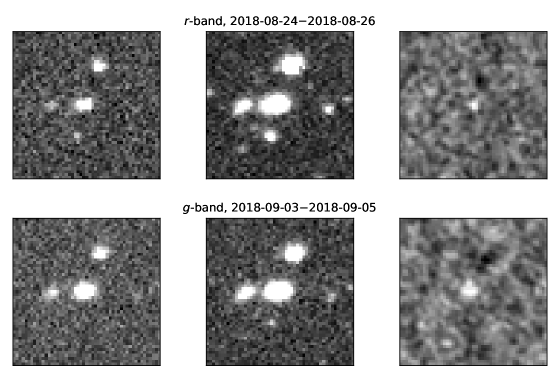
Figure 6: Sample pre-explosion subtractions of deep PTF/iPTF references from ZTF science images stacked in 3-day bins (see Section 2.4). Each cutout is centered on the location of SN2018gep. The subtractions show clear emission at the location of the SN in both $g$ and $r$-bands days to weeks before the discovery of the SN in ZTF.

Using these newly constructed deep subtractions, PSF photometry was performed at the location of SN2018gep using the PSF of the science images. To estimate the uncertainty on the flux measurements made on these subtractions, we employed a Monte Carlo technique, in which thousands of PSF fluxes were measured at random locations on the image, and the PSF-flux uncertainty was taken to be the 1$\sigma$ dispersion in these measurements. We loaded this photometry into a local instance of SkyPortal (van der Walt et al., 2019), an open-source web application that interactively displays astronomical datasets for annotation, analysis, and discovery.

We detected significant flux excesses at the location of SN2018gep in both $g$ and $r$ bands in the weeks preceding $t_{0}$ (i.e. its first detection in single-epoch ZTF subtractions). The effective dates of these extended pre-discovery detections are determined by taking an inverse-flux variance weighted average of the input image dates. The detections in the week leading up to explosion are $m_{g}\sim m_{r}\approx 22$, which is approximately the magnitude limit of the coadd subtractions. However, in an $r$-band stack of images from August 24–26 (inclusive), we detect emission at $m_{r}\sim 21.5$ at $5\sigma$ above the background.

Assuming that the rapid rise we detected was close to the time of explosion, this is the first definitive detection of pre-explosion emission in a Ic-BL SN. There was a tentative detection in another source, PTF 11qcj (Corsi et al., 2014), 1.5 and 2.5 years prior to the SN. In Section 4 we discuss possible mechanisms for this emission, and conclude that it is likely related to a period of eruptive mass-loss immediately prior to the explosion. We note that it is unlikely that this variability arises from AGN activity, due to the properties of the host galaxy (Section 3.3).

With forced photometry and faint detections from stacked images and deep references, we can construct a light curve that extends weeks prior to the rapid rise in the light curve, shown in Figure 7.

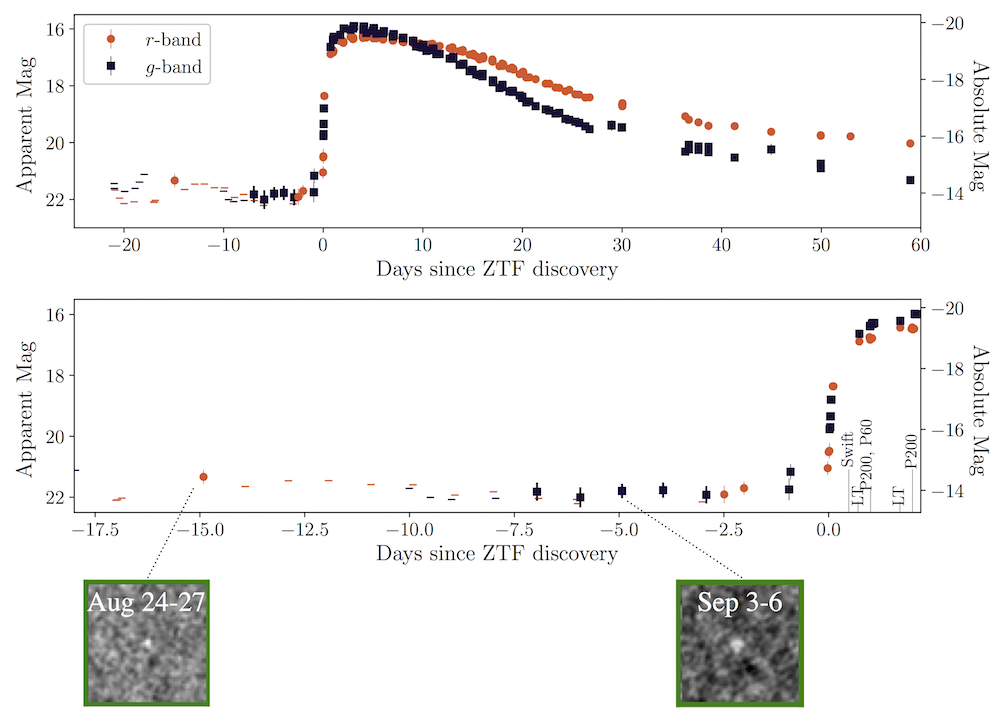
Figure 7: Full $r$ and $g$-band light curves of SN2018gep. 3-$\sigma$ upper limits are shown as horizontal lines. Points at $t<0$ are from 3-day stacks of ZTF/P48 data as described in Section 2.4. Sample subtractions from two of these stacks are shown in the bottom row.

2.5 Radio follow-up

We observed the field of SN2018gep with the Karl G. Jansky Very Large Array (VLA) on three epochs: on 2018 September 14 UT under the Program ID VLA/18A-242 (PI: D. Perley; Ho et al. 2018b), and on 2018 September 25 and 2018 November 23 UT under the Program ID VLA/18A-176 (PI: A. Corsi). We used 3C286 for flux calibration, and J1640+3946 for gain calibration. The observations were carried out in X- and Ku-band (nominal central frequencies of 9 $\rm GHz$ and 14 $\rm GHz$, respectively) with a nominal bandwidth of 2 $\rm GHz$. The data were calibrated using the automated VLA calibration pipeline available in the CASA package (McMullin et al., 2007) then inspected for further flagging. The CLEAN procedure (Högbom, 1974) was used to form images in interactive mode. The image rms and the radio flux at the location of SN2018gep were measured using imstat in CASA. Specifically, we report the maximum flux within pixels contained in a circular region centered on the optical position of SN2018gep with radius comparable to the FWHM of the VLA synthesized beam at the appropriate frequency. The source was detected in the first two epochs, but not in the third (see Table 2). As we discuss in Section 4, the first two epochs were conducted in a different array configuration than the third epoch, and may have had a contribution from host galaxy light.

We also obtained three epochs of observations with the AMI large array (AMI-LA; Zwart et al. 2008; Hickish et al. 2018), on UT 2018 Sept 12, 2018 Sept 23, and 2018 Oct 20. AMI-LA is a radio interferometer comprised of eight, 12.8 m diameter that extends from 18 m up to 110 m in length and operates with a 5 GHz bandwidth around a central frequency of 15.5 GHz.

We used a custom AMI data reduction software package reduce_dc (e.g. Perrott et al. 2013) to perform initial data reduction, flagging, and calibration of phase and flux. Phase calibration was conducted using short interleaved observations of J1646+4059, and for absolute flux calibration we used 3C286. Additional flagging and imaging were performed using CASA. All three observations resulted in null-detections with 3-$\sigma$ upper limits of $\approx 120\,\mu$Jy in the first two observations, and a 3-$\sigma$ upper limit of $\approx 120\,\mu$Jy in the last observation.

Finally, we observed at higher frequencies using the Submillimeter Array (SMA; Ho et al. 2004) on UT 2018 Sep 15 under its target-of-opportunity program. The project ID was 2018A-S068. Observations were performed in the sub-compact configuration using seven antennas. The observations were performed using RxA and RxB receivers tuned to LO frequencies of 225.55 GHz and 233.55 GHz respectively, providing 32 GHz of continuous bandwidth ranging from 213.55 GHz to 245.55 GHz with a spectral resolution of 140.0 kHz per channel. The atmospheric opacity was around 0.16-0.19 with system temperatures around 100-200 $\rm K$. The nearby quasars 1635+381 and 3C345 were used as the primary phase and amplitude gain calibrators with absolute flux calibration performed by comparison to Neptune. Passband calibration was derived using 3C454.3. Data calibration was performed using the MIR IDL package for the SMA, with subsequent analysis performed in MIRIAD (Sault et al., 1995). For the flux measurements, all spectral channels were averaged together into a single continuum channel and an rms of 0.6 mJy was achieved after 75 minutes on-source.

The full set of radio and sub-millimeter measurements are listed in Table 2.

Table 2: Radio flux density measurements for SN2018gep.

Start Time	$\Delta t$	Instrument	$\nu$	$f_{\nu}$	$L_{\nu}$	$\theta_{\mathrm{FWHM}}$	Int. time
(UTC)	(days)		(GHz)	($\mu$Jy)	(erg $\rm s^{-1}$ $\rm Hz^{-1}$)	′′	(hr)
2018-09-12 17:54	3.6	AMI	15	$<120$	$<2.9\times 10^{27}$	$43.53\times 30.85$	4
2018-09-23 15:35	14.5	AMI	15	$<120$	$<2.9\times 10^{27}$	$39.3\times 29.29$	4
2018-10-20 14:01	41.4	AMI	15	$<120$	$<2.9\times 10^{27}$	$43.53\times 30.85$	4
2018-09-15 02:33	6.0	SMA	230	$<590$	$<1.4\times 10^{28}$	$4.828\times 3.920$	1.25
2018-09-14 01:14	4.9	VLA	9.7	$34\pm 4$	$8.3\times 10^{26}$	$7.06\times 5.92$	0.5
2018-09-25 00:40	15.9	VLA	9	$24.4\pm 6.8$	$6.0\times 10^{26}$	$7.91\times 6.89$	0.7
2018-09-25 00:40	15.9	VLA	14	$26.8\pm 6.8$	$6.6\times 10^{26}$	$4.73\times 4.26$	0.5
2018-11-23 13:30	75.4	VLA	9	$<16$	$<3.9\times 10^{26}$	$3.52\times 2.08$	0.65
2018-11-23 13:30	75.4	VLA	14	$<17$	$<4.2\times 10^{26}$	$2.77\times 1.32$	0.65

Note. — For VLA measurements: The quoted errors are calculated as the quadrature sums of the image rms, plus a 5% nominal absolute flux calibration uncertainty. When the peak flux density within the circular region is less than three times the RMS, we report an upper limit equal to three times the RMS of the image. For AMI measurements: non-detections are reported as 3-$\sigma$ upper limits. For SMA measurements: non-detections are reported as a 1-$\sigma$ upper limit.

2.6 X-ray follow-up

We observed the position of SN2018gep with Swift/XRT from $\Delta t\approx 0.4$–14 $\rm day$. The source was not detected in any epoch. To measure upper limits, we used web-based tools developed by the Swift-XRT team (Evans et al., 2009). For the first epoch, the 3-$\sigma$ upper limit was 0.003 ct/s. To convert the upper limit from count rate to flux, we assumed a Galactic neutral hydrogen column density of $1.3\times 10^{20}\,\mbox{$\rm cm^{-2}$}$, and a power-law spectrum with photon index $\Gamma=2$. This gives an unabsorbed 0.3–10 $\rm keV$ flux of $<9.9\times 10^{-14}\,\mbox{$\rm erg$}\,\mbox{$\rm cm^{-2}$}\,\mbox{$\rm s^{-1}$}$, and $L_{X}<2.5\times 10^{41}\,\mbox{$\rm erg$}\,\mbox{$\rm s^{-1}$}$.

We obtained two epochs of observations with the Advanced CCD Imaging Spectrometer (ACIS; Garmire et al. 2003) on the Chandra X-ray Observatory via our approved program (Proposal No. 19500451; PI: Corsi). The first epoch began at 9:25 UTC on 10 October 2018 ($\Delta t\approx 15\,\mbox{$\rm day$}$) under ObsId 20319 (integration time 12.2 ks), and the second began at 21:31 UTC on 4 December 2018 ($\Delta t\approx 70\,\mbox{$\rm day$}$) under ObsId 20320 (integration time 12.1 ks). No X-ray emission is detected at the location of SN2018gep in either epoch, with 90% upper limits on the 0.5–7.0 keV count rate of $\approx 2.7\times 10^{-4}\,\mathrm{ct}\,\mbox{$\rm s^{-1}$}$. Using the same values of hydrogen column density and power-law photon index as in our XRT measurements, we find upper limits on the unabsorbed 0.5–7 $\rm keV$ X-ray flux of $<3.2\times 10^{-15}$ erg cm^-2 s^-1, or (for a direct comparison to the XRT band) a 0.3–10 $\rm keV$ X-ray flux of $<4.2\times 10^{-15}$ erg cm^-2 s^-1. This corresponds to a 0.3–10 $\rm keV$ luminosity upper limit of $L_{X}<1.0\times 10^{40}\,\mbox{$\rm erg$}\,\mbox{$\rm s^{-1}$}$.

2.7 Search for prompt gamma-ray emission

We created a tool to search for prompt gamma-ray emission (GRBs) from Fermi-GBM (Gruber et al., 2014; von Kienlin et al., 2014; Narayana Bhat et al., 2016), the Swift Burst Alert Telescope (BAT; Barthelmy et al. 2005), and the IPN, which we have made available online. We did not find any GRB consistent with the position and $t_{0}$ of SN2018gep.

Our tool also determines whether a given position was visible to BAT and GBM at a given time, using the spacecraft pointing history. We use existing code to determine the BAT history. We find that the position of SN2018gep was in the BAT field-of-view from UTC 03:13:40 to 03:30:38, before Swift slewed to another location.

We also find that at $t_{0}$ SN2018gep was visible to the Fermi Gamma-Ray Burst Monitor (GBM; Meegan et al. 2009). We ran a targeted GRB search in 10–1000 $\rm keV$ Fermi/GBM data from three hours prior to $t_{0}$ to half an hour after $t_{0}$. We use the soft template, which is a smoothly broken power law with low-energy index $-1.9$ and high-energy index $-2.7$, and an SED peak at 70 $\rm keV$. The search methodology (and parameters of the other templates) are described in Blackburn et al. (2015) and Goldstein et al. (2016). No signals with a consistent location were found. For the 100 s integration time, the fluence upper limit is $2\times 10^{-6}\,\mbox{$\rm erg$}\,\mbox{$\rm cm^{-2}$}$. This limit corresponds to a 10–1000 $\rm keV$ isotropic energy release of $E_{\mathrm{\gamma,iso}}<4.9\times 10^{48}\,\mbox{$\rm erg$}$. Limits for different spectral templates and integration times are shown in Figure 8.

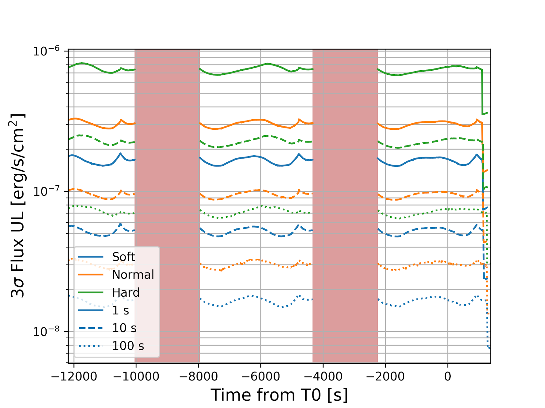
Figure 8: 3-$\sigma$ upper limits from GBM GRB search, which we performed for three hours prior to $t_{0}$. The red vertical bars indicate epochs when GBM was not taking data due to passing through the South Atlantic Anomaly. The time of $t_{0}$ was estimated from a fit to the early data (Figure 7), and is $26\pm 5$ minutes prior to the first detection.

2.8 Host galaxy data

We measure line fluxes using the Keck optical spectrum obtained at $\Delta t\approx 61\,\mbox{$\rm day$}$ (Figure 25). We model the local continuum with a low-order polynomial and each emission line by a Gaussian profile of FHWM $\sim 5.3$ Å. This is appropriate if Balmer absorption is negligible, which is generally the case for starburst galaxies. For the host of SN2018gep, the Balmer decrement between H$\beta$, H$\gamma$ and H$\delta$ does not show any excess with respect to the expected values in Osterbrock & Ferland (2006). The resulting line fluxes are listed in Table 7.

We retrieved archival images of the host galaxy from Galaxy Evolution Explorer (GALEX) Data Release (DR) 8/9 (Martin et al., 2005), Sloan Digital Sky Survey (SDSS) DR9 (Ahn et al., 2012), Panoramic Survey Telescope And Rapid Response System (PanSTARRS, PS1) DR1 (Chambers et al., 2016), Two-Micron All Sky Survey (2MASS; Skrutskie et al., 2006), and Wide-Field Infrared Survey Explorer (WISE; Wright et al., 2010). We also used UVOT photometry from Swift, and NIR photometry from the Canada-France-Hawaii Telescope Legacy Survey (CFHTLS; Hudelot et al., 2012).

The images are characterized by different pixel scales (e.g., SDSS $0\farcs 40$/px, GALEX $1\farcs$/px) and different point spread functions (e.g., SDSS/PS1 1–$2^{\prime\prime}$, WISE/W2 $6\farcs 5$). To obtain accurate photometry, we use the matched-aperture photometry software package Lambda Adaptive Multi-Band Deblending Algorithm in R (LAMBDAR; Wright et al., 2016) that is based a photometry software package developed by Bourne et al. (2012). To measure the total flux of the host galaxy, we defined an elliptical aperture that encircles the entire galaxy in the SDSS/$r^{\prime}$-band image. This aperture was then convolved in LAMBDAR with the point-spread function of a given image that we specified directly (GALEX and WISE data) or that we approximated by a two-dimensional Gaussian (2MASS, SDSS and PS1 images). After instrumental magnitudes were measured, we calibrated the photometry against instrument-specific zeropoints (GALEX, SDSS and PS1 data), or as in the case of 2MASS and WISE images against a local sequence of stars from the 2MASS Point Source Catalogue and the AllWISE catalogue. The photometry from the UVOT images were extracted with the command uvotsource in HEAsoft and a circular aperture with a radius of $8^{\prime\prime}$. The photometry of the CFHT/WIRCAM data was done performed the software tool presented in Schulze et al. (2018b). To convert the 2MASS, UVOT, WIRCAM and WISE photometry to the AB system, we applied the offsets reported in Blanton, & Roweis (2007), Breeveld et al. (2011) and Cutri et al. (2013). The resulting photometry is summarized in Table 8.

3 Basic properties of the explosion and its host galaxy

The observations we presented in Section 2 constitute some of the most detailed early-time observations of a stripped-envelope SN to date. In this section we use this data to derive basic properties of the explosion: the evolution of bolometric luminosity, radius, and effective temperature over time (Section 3.1), the velocity evolution of the photosphere and the density and composition of the ejecta as measured from the spectra (Section 3.2), and the mass, metallicity, and SFR of the host galaxy (Section 3.3). These properties are summarized in Table 1.

3.1 Physical evolution from blackbody fits

By interpolating the UVOT and ground-based photometry, we construct multi-band SEDs and fit a Planck function on each epoch, to measure the evolution of luminosity, radius, and effective temperature. To estimate the uncertainties, we perform a Monte Carlo simulation with 600 trials, each time adding noise corresponding to a 15% systematic uncertainty on each data point, motivated by the need to obtain a combined $\chi^{2}$/dof $\sim$ 1 across all epochs. The uncertainties for each parameter are taken as the 16-to-84 percentile range from this simulation. The SED fits are shown in Appendix A, and the resulting evolution in bolometric luminosity, photospheric radius, and effective temperature is listed in Table 3. We plot the physical evolution in Figure 9, with a comparison to iPTF16asu and AT2018cow.

The bolometric luminosity peaks between $\Delta t=0.5\,\mbox{$\rm day$}$ and $\Delta t=3\,\mbox{$\rm day$}$, at $>3\times 10^{44}\,\mbox{$\rm erg$}\,\mbox{$\rm s^{-1}$}$. In Figure 10 we compare this peak luminosity and time to peak luminosity with several classes of stellar explosions. As in iPTF16asu, the bolometric luminosity falls as an exponential at late times ($t>10\,\mbox{$\rm day$}$). The total integrated UV and optical ($\approx 2000$–$9000$Å) blackbody energy output from $\Delta t=0.5$–40 $\rm day$ is $\sim 10^{50}\,\mbox{$\rm erg$}$, similar to that of iPTF16asu.

The earliest photospheric radius we measure is $\sim 20\,$AU, at $\Delta t=0.05\,\mbox{$\rm day$}$. Until $\Delta t\approx 17\,\mbox{$\rm day$}$ the radius expands over time with a very large inferred velocity of $v\approx 0.1c$. After that, it remains flat, and even appears to recede. This possible recession corresponds to a flattening in the temperature at $\sim 5000\,\mbox{$\rm K$}$, which is the recombination temperature of carbon and oxygen. This effect was not seen in iPTF16asu, which remained hotter (and more luminous) for longer. Finally, the effective temperature rises before falling as $\sim t^{-1}$. We interpret these properties in the context of shock-cooling emission in Section 4.

Table 3: Physical evolution of AT2018gep from blackbody fits.

$\Delta t$	$L(10^{10}L_{\odot})$	$R$ (AU)	$T$ (kK)
$0.05$	$0.04^{+0.04}_{-0.02}$	$21^{+14}_{-6}$	$13^{+5}_{-4}$
$0.48$	$7.4^{+8.6}_{-4.1}$	$22^{+7}_{-5}$	$46^{+16}_{-13}$
$0.73$	$4.5^{+5.5}_{-2.8}$	$31^{+11}_{-6}$	$35^{+12}_{-11}$
$1.0$	$2.2^{+2.1}_{-1.2}$	$46^{+18}_{-9}$	$24^{+6}_{-6}$
$1.7$	$3.5^{+4.2}_{-2.1}$	$46^{+22}_{-10}$	$27^{+9}_{-8}$
$2.7$	$1.3^{+1.2}_{-0.4}$	$78^{+22}_{-20}$	$16^{+5}_{-3}$
$3.2$	$3.5^{+2.2}_{-1.3}$	$50^{+14}_{-8}$	$26^{+6}_{-5}$
$3.8$	$2.9^{+1.7}_{-0.8}$	$56^{+11}_{-11}$	$23^{+5}_{-3}$
$4.7$	$1.7^{+0.7}_{-0.3}$	$69^{+16}_{-14}$	$18^{+3}_{-2}$
$5.9$	$0.88^{+0.17}_{-0.08}$	$100^{+14}_{-21}$	$13^{+1}_{-0}$
$8.6$	$0.46^{+0.08}_{-0.06}$	$220^{+46}_{-39}$	$7.4^{+0.6}_{-0.5}$
$9.6$	$0.33^{+0.04}_{-0.03}$	$200^{+33}_{-24}$	$7.1^{+0.4}_{-0.4}$
$10.0$	$0.31^{+0.04}_{-0.03}$	$210^{+34}_{-28}$	$6.9^{+0.4}_{-0.4}$
$11.0$	$0.28^{+0.04}_{-0.03}$	$220^{+35}_{-33}$	$6.5^{+0.4}_{-0.3}$
$13.0$	$0.25^{+0.04}_{-0.03}$	$260^{+50}_{-42}$	$5.8^{+0.3}_{-0.3}$
$14.0$	$0.22^{+0.04}_{-0.03}$	$270^{+60}_{-47}$	$5.5^{+0.4}_{-0.3}$
$16.0$	$0.17^{+0.04}_{-0.03}$	$260^{+76}_{-58}$	$5.3^{+0.5}_{-0.5}$
$18.0$	$0.15^{+0.04}_{-0.02}$	$300^{+77}_{-64}$	$4.7^{+0.4}_{-0.4}$
$21.0$	$0.11^{+0.03}_{-0.02}$	$250^{+83}_{-58}$	$4.7^{+0.4}_{-0.4}$
$25.0$	$0.073^{+0.02}_{-0.013}$	$240^{+95}_{-85}$	$4.5^{+0.9}_{-0.5}$
$38.0$	$0.034^{+0.012}_{-0.007}$	$180^{+86}_{-55}$	$4.2^{+0.6}_{-0.5}$

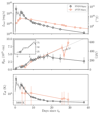
Figure 9: Evolution of blackbody properties (luminosity, radius, temperature) over time compared to the Ic-BL SN iPTF16asu and the luminous fast-rising optical transient AT2018cow. The light gray circles are derived from optical data only. The outlined circles are derived from UV and optical data. Middle panel: dotted line shows $v=0.1c$. Note that $R\neq 0$ at $t_{0}$, and instead $R(t=0)=3\times 10^{14}\,\mbox{$\rm cm$}$. Due to the scaling of our plot we do not show the radius evolution of AT2018cow, which drops from $8\times 10^{14}\,\mbox{$\rm cm$}$ to $10^{14}\,\mbox{$\rm cm$}$ on this timescale. Bottom panel: dotted horizontal line shows 5000 $\rm K$, the recombination temperature for carbon and oxygen. Once this temperature is reached, the photosphere flattens out (and potentially begins to recede).

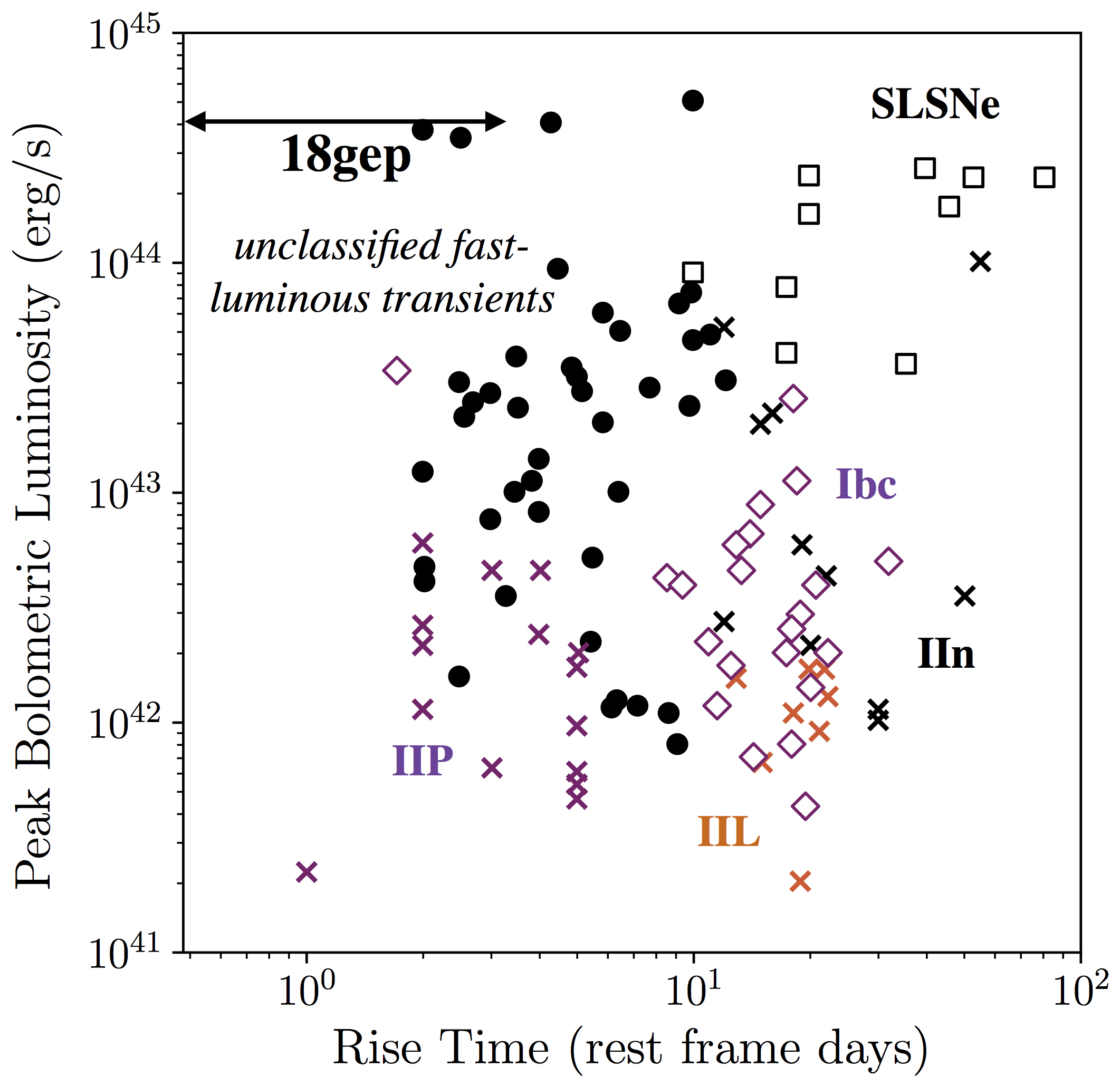
Figure 10: Rise to peak bolometric luminosity compared to other classes of transients. Modified from Figure 1 in Margutti et al. (2019).

3.2 Spectral evolution and velocity measurements

3.2.1 Comparisons to early spectra in the literature

We obtained nine spectra of SN2018gep in the first five days after discovery. These early spectra are shown in Figure 11, when the effective temperature declined from 50,000 $\rm K$ to 20,000 $\rm K$. To our knowledge, our early spectra have no analogs in the literature, in that there has never been a spectrum of a stripped-envelope SN at such a high temperature (excluding spectra during the afterglow phase of GRBs). Two of the earliest spectra in the literature, one at $\Delta t=2\,\mbox{$\rm day$}$ for Type Ic SN PTF10vgv (Corsi et al., 2012) and one at $\Delta t=3\,\mbox{$\rm day$}$ for Type Ic SN PTF12gzk (Ben-Ami et al., 2012) are redder and exhibit more features than the spectrum of SN2018gep. We show the comparison in Figure 11.

At $\Delta t\approx 4\,\mbox{$\rm day$}$, a “W” feature emerges in the rest-frame wavelength range 3800–4350 Å. In the second-from-bottom panel of Figure 11 we make a comparison to “W” features seen in SN 2008D (e.g. Modjaz et al. 2009), which was a Type Ib SN associated with an X-ray flash (Mazzali et al., 2008), and in a typical pre-max stripped-envelope superluminous supernova (Type I SLSN; Moriya et al. 2018; Gal-Yam 2019). The absorption lines are broadened much more than in PTF12dam (Nicholl et al., 2013) and probably more than in SN2008D as well. Finally, SN2018gep cooled more slowly than SN 2008D: only after 4.25 days did it reach the temperature that SN 2008D reached after $<2$ days.

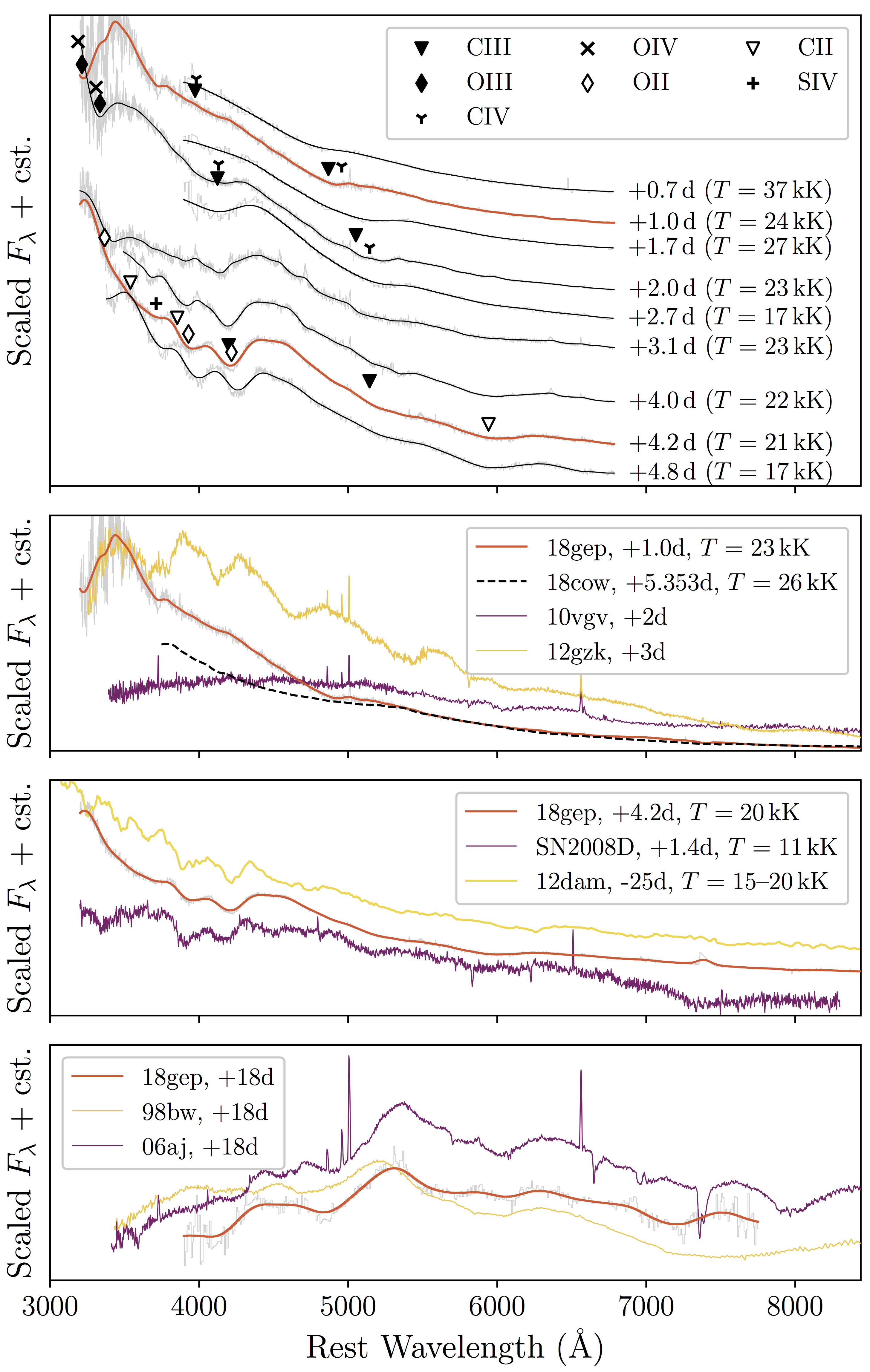
Figure 11: Top panel: spectra of SN2018gep taken in the first five days. Broad absorption features are consistent with ionized carbon and oxygen, which evolve redward with time. Second-from-top panel: an early spectrum of 18gep compared to spectra from other stellar explosions at a comparable phase. Second-from-bottom panel: The spectrum at $\Delta t=4.2\,\mbox{$\rm day$}$ shows a “W” feature, which we compare to similar “W” features seen in an early spectrum of SN2008D from Modjaz et al. (2009), and a typical pre-max spectrum of a SLSN-I (PTF12dam, from Nicholl et al. 2013). We boost the SLSN spectrum by an additional expansion velocity of $\sim 15000$ km s^-1, and apply reddening of $E(B-V)=0.63$ to SN 2008D. Weak features in the red are also similar to what are seen in PTF12dam, and are consistent with arising from CII and CIII lines, following the analysis of Gal-Yam (2019). The lack of narrow carbon features as well as the smooth spectrum below 3700 Å suggest a large velocity dispersion leading to significant line broadening, compared to the intrinsically narrow features observed in SLSNe-I (Gal-Yam, 2019; Quimby et al., 2018). Bottom panel: a spectrum of 18gep when it resembled an ordinary Ic-BL SN, compared to spectra at similar phases of Ic-BL SNe accompanying GRBs.

3.2.2 Origin of the “W” feature

The lack of comparison data at such early epochs (high temperatures) motivated us to model one of the early spectra, in order to determine the composition and density profile of the ejecta. We used the spectral synthesis code JEKYLL (Ergon et al., 2018), configured to run in steady-state using a full NLTE-solution. An inner blackbody boundary was placed at an high continuum optical depth ($\sim$50), and the temperature at this boundary was iteratively determined to reproduce the observed luminosity. The atomic data used is based on what was specified in Ergon et al. (2018), but has been extended as described in Appendix C. We explored models with C/O (mass fractions: 0.23/0.65) and O/Ne/Mg (mass fractions: 0.68/0.22/0.07) compositions taken from a model by Woosley & Heger (2007) and a power-law density profile, where the density at the inner border was adjusted to fit the observed line velocities. Except for the density at the inner border, various power-law indices where also explored, but in the end an index of -9 worked out best.

Figures 12 and 13 show the model with the best overall agreement with the spectra and the SED (as listed in Table 6 the spectrum was obtained at high airmass, making it difficult to correct for telluric features). The model has a C/O composition, an inner border at 22,000 $\rm km$ $\rm s^{-1}$ (corresponding to an optical depth of $\sim$50), a density of 4$\times$10^-12 g cm^-3 at this border and a density profile with a power-law index of $-9$. In Figure 12 we show that the model does a good job of reproducing both the spectrum and the SED of SN2018gep. In particular, it is interesting to note that the “W” feature seem to arise naturally in C/O material at the observed conditions. A similar conclusion was reached by Dessart (2019), whose magnetar-powered SLSN-I models, calculated using the NLTE code CMFGEN, show the “W” feature even when non-thermal processes where not included in the calculation (as in our case).

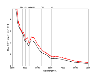
Figure 12: Observed spectrum (red) at 4.2 $\rm day$, compared to our model spectrum (black) from the spectral synthesis code JEKYLL configured to run in steady-state using a full NLTE solution. The model has a C/O composition, an inner border at 22,000 $\rm km$ $\rm s^{-1}$, a density of $4\times 10^{-12}\,\mbox{$\rm g$}\,\mbox{$\rm cm^{-3}$}$, and a density profile with a power-law index of $-9$. The absolute (but not relative) flux of the spectrum was calibrated using the interpolated P48 g and r magnitudes. We also show the O II, C II, C III and Si IV lines discussed in the text shifted to the velocity of the model photosphere.

In the model, the “W” feature mainly arises from the O II 2p²(3P)3s 4P $\leftrightarrow$ 2p²(3P)3p 4D^∘ (4639–4676 Å), O II 2p²(3P)3s 4P $\leftrightarrow$ 2p²(3P)3p 2D (4649 Å) and O II 2p²(3P)3s 4P $\leftrightarrow$ 2p²(3P)3p 4P^∘ (4317–4357 Å) transitions. The departure from LTE is modest in the line-forming region, and the departure coefficients for the O II states are small. The spectrum redward of the “W” feature is shaped by carbon lines, and the features near 5700 and 6500 Å arise from the C II 3s 2S $\leftrightarrow$ 3p 2P^∘ (6578,6583 Å) and C III 2s3p 1P^∘ $\leftrightarrow$ 2s3d 1D (5696 Å) transitions, respectively. In the model, the C II feature is too weak, suggesting that the ionization level is too high in the model. There is also a contribution from the C III 2s3s 3S $\leftrightarrow$ 2s3p 3P^∘ (4647–4651 Å) transition to the red part of the “W” feature, which could potentially be what is seen in the spectra from earlier epochs. In addition, there is a contribution from Si IV 4s 2S $\leftrightarrow$ 4p 2P^∘ (4090, 4117 Å) near the blue side of the “W” feature, which produce a distinct feature in models with lower velocities and which could explain the observed feature on the blue side of the “W” feature.

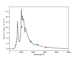
Figure 13: Comparison of model (filled circles) and observed (unfilled circles) mean fluxes through the Swift UVW1 (blue), UVM2 (green), UVW2 (red), and the SDSS u (black), g (green) and r (red) filters. We also show the model spectrum in black.

In spite of the overall good agreement, there are also some differences between the model and the observations. In particular the model spectrum is bluer and the velocities are higher. These two quantities are in tension and a better fit to one of them would result in a worse fit to the other. As mentioned above, the ionization level might be too high in the model, which suggests that the temperature might be too high as well. It should be noted that adding host extinction (which is assumed to be zero) or reducing the distance (within the error bars) would help in making the model redder (in the observer frame), and the latter would also help in reducing the temperature. The (modest) differences between the model and the observations could also be related to physics not included in the model, like a non-homologous velocity field, departures from spherical asymmetry, and clumping.

The total luminosity of the model is 6.2$\times$10⁴³ erg s^-1, the photosphere is located at $\sim$33,000 $\rm km$ $\rm s^{-1}$ and the temperature at the photosphere is $\sim$17,500 $\rm K$, which is consistent with the values estimated from the blackbody fits (although the blackbody radius and temperature fits refer to the thermalization layer). As mentioned, we have also tried models with a O/Ne/Mg composition. However, these models failed to reproduce the carbon lines redwards of the “W” feature. We therefore conclude that the (outer) ejecta probably has a C/O-like composition, and that this composition in combination with a standard power-law density profile reproduce the spectrum of SN2018gep at the observed conditions (luminosity and velocity) 4.2 days after explosion.

In our model, the broad feature seen in our Swift UVOT grism spectrum is dominated by the strong Mg II (2796,2803 Å) resonance line. However, a direct comparison is not reliable because the ionization is probably lower at this epoch than what we consider for our model.

3.2.3 Photospheric velocity from Ic-BL spectra

At $\Delta t\gtrsim 7.8\,\mbox{$\rm day$}$, the spectra of SN2018gep qualitatively resemble those of a stripped-envelope SN. We measure velocities using the method in Modjaz et al. (2016), which accommodates blending of the Fe II$\lambda$5169 line (which has been shown to be a good tracer of photospheric velocity; Branch et al. 2002) with the nearby Fe II$\lambda\lambda$4924,5018 lines.

At earlier times, when the spectra do not resemble typical Ic-BL SNe, we use our line identifications of ionized C and O to measure velocities. As shown in Figure 14, the velocity evolution we measure is comparable to that seen in Ic-BL SNe associated with GRBs (more precisely, low-luminosity GRBs; LLGRBs) which are systematically higher than those of Ic-BL SNe lacking GRBs (Modjaz et al., 2016). However, as discussed in Section 2.7, no GRB was detected.

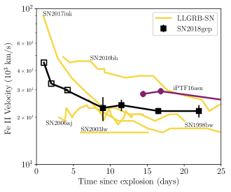
Figure 14: Velocity evolution over time as measured from spectral absorption features. Open symbols for SN2018gep come from C/O velocities measured from line minima. Closed symbols come from the Fe II feature in the Ic-BL spectra. The velocities are comparable to those measured for Ic-BL SNe associated with low-luminosity GRBs (LLGRBs). The velocity evolution for SN2017iuk is taken from Izzo et al. (2019). Velocities for iPTF16asu are taken from Whitesides et al. (2017). Velocities for the other Ic-BL SNe are taken from Modjaz et al. (2016) and shifted from V-band max using data from Galama et al. (1998), Campana et al. (2006), Malesani et al. (2004), and Bufano et al. (2012).

3.3 Properties of the host galaxy

We infer a star-formation rate of $0.09\pm 0.01~{}M_{\odot}\,{\rm yr}^{-1}$ from the H$\alpha$ emission line using the Kennicutt (1998) relation converted to use a Chabrier initial mass function (Chabrier, 2003; Madau, & Dickinson, 2014). We note that this is a lower limit as the slit of the Keck observation did not enclose the entire galaxy. We estimate a correction factor of 2–3: the slit diameter in the Keck spectra was 1.0”, and the extraction radius was $\sim 1.75^{\prime\prime}$ in the February observation and $\sim 1.21^{\prime\prime}$ in the March observation. The host diameter is roughly 4”.

We derive an electron temperature of $13,100^{+900}_{-1000}\,\mbox{$\rm K$}$ from the flux ratio between [O III]$\lambda$4641 and [O III]$\lambda$5007, using the software package PyNeb version 1.1.7 (Luridiana et al., 2015). In combination with the flux measurements of [O II]$\lambda\lambda$3226,3729, [O III]$\lambda$4364, [O III]$\lambda$4960, [O III]$\lambda$5008, and H$\beta$, we infer a total oxygen abundance of $8.01^{+0.10}_{-0.09}$ (statistical error; using Eqs. 3 and 5 in Izotov et al. 2006). Assuming a solar abundance of 8.69 (Asplund et al., 2009), the metallicity of the host is $\sim 20\%$ solar.

We also compute the oxygen abundance using the strong-line metallicity indicator O3N2 (Pettini, & Pagel, 2004) with the updated calibration reported in Marino et al. (2013). The oxygen abundance in the O3N2 scale is $8.05\pm 0.01\,({\rm stat})\pm 0.10\,({\rm sys})$.

We also estimate mass and star-formation rate by modeling the host SED; see Appendix D for a table of measurements, and details on where we obtained them. We use the software package LePhare version 2.2 (Arnouts et al., 1999; Ilbert et al., 2006). We generated $3.9\times 10^{6}$ templates based on the Bruzual & Charlot (2003) stellar population-synthesis models with the Chabrier initial mass function (IMF; Chabrier, 2003). The star formation history (SFH) was approximated by a declining exponential function of the form $\exp\left(−t/\tau\right)$, where $t$ is the age of the stellar population and $\tau$ the e-folding time-scale of the SFH (varied in nine steps between 0.1 and 30 Gyr). These templates were attenuated with the Calzetti attenuation curve (Calzetti et al., 2000) varied in 22 steps from $E(B-V)=0$ to 1 mag .

As shown in Figure 15, the SED is well characterized by a galaxy mass of $\log M/M_{\odot}=8.11^{+0.07}_{-0.08}$ and an attenuation-corrected star-formation rate of $0.12^{+0.08}_{-0.05}\,M_{\odot}\,\mbox{$\rm yr^{-1}$}$. The derived star-formation rate is comparable to measurement inferred from H$\alpha$. The attenuation of the SED is marginal, with $E(B-V)_{\rm star}=0.05$, and consistent with the negligible Balmer decrement 2.8.

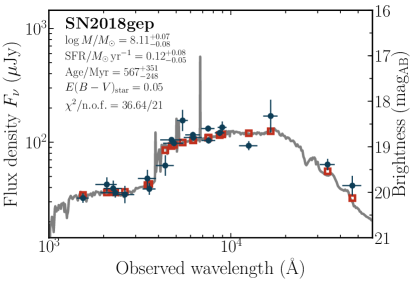
Figure 15: The spectral energy distribution of the host galaxy of SN2018gep from 1,000 to 60,000 Å and the best fit (solid line) in the observer frame. Filled data points represent photometric measurements. The error bars in the ‘x’ direction indicate the full-width half maximum of each filter response function. The open data points signify the model-predicted magnitudes. The quoted values of the host properties represent the median values and the corresponding 1-$\sigma$ errors.

Figure 16 shows that the host galaxy of SN2018gep is even more low-mass and metal-poor than the typical host galaxies of Ic-BL SNe, which are low-mass and metal-poor compared to the overall core collapse SN population to begin with. The figure uses data for 28 Ic-BL SNe from PTF and iPTF (Modjaz et al., 2019; Taddia et al., 2019) and a sample of 11 long-duration GRBs (including LLGRBs, all at $z<0.3$). We measured the emission lines from the spectra presented in Taddia et al. (2019) and used line measurements reported in Modjaz et al. (2019) for objects with missing line fluxes. The photometry was taken from Schulze, S. et al. (in preparation). Photometry and spectroscopy were taken from a variety of sources. The oxygen abundances were measured in the O3N2 scale like for SN2018gep and their SEDs were modelled with the same set of galaxy templates. For reference, the mass and SFR of the host of AT2018cow was $1.4\times 10^{9}\,\mbox{$M_{\odot}$}$ and $0.22\,\mbox{$M_{\odot}$}\,\mbox{$\rm yr^{-1}$}$, respectively (Perley et al., 2019a). The mass and SFR of the host of iPTF16asu was $4.6^{+6.5}_{-2.3}\times 10^{8}\,\mbox{$M_{\odot}$}$ and $0.7\,\mbox{$M_{\odot}$}\,\mbox{$\rm yr^{-1}$}$, respectively (Whitesides et al., 2017).

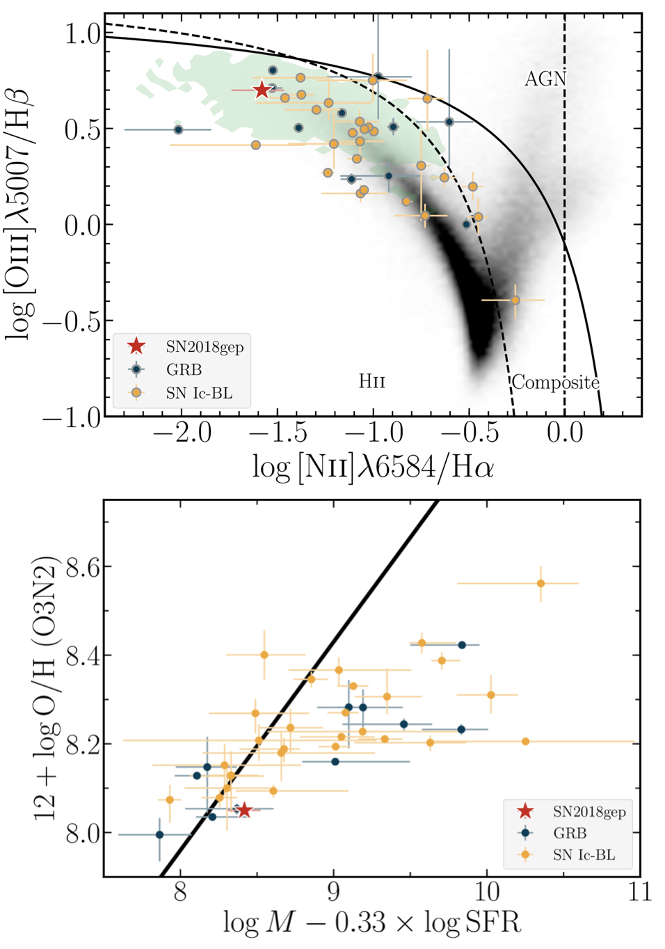
Figure 16: Top: BPT diagram. The host of SN2018gep is a low-metallicity galaxy with an intense ionizing radiation field (green shaded region indicates extreme emission line galaxies). The majority of Ic-BL SNe and long-duration GRBs are found in more metal enriched galaxies (parameterized by [N II]/H$\alpha$), and galaxies with less intense radiation fields (parameterized by [O III]/H$\alpha$). Field galaxies from SDSS DR15 are shown as a background density distribution. The thick solid line separates star formation- and AGN-dominated galaxies (Kewley et al., 2001). The thick dashed lines encircle the region of composite galaxies (Kauffmann et al., 2003). Bottom: The mass-metallicity-star-formation-rate plane. The bulk of the the SN-Ic-BL and GRB host populations are found in hosts that are more metal enriched. For reference, the host of AT2018cow had $\log{M}-0.33\times\log{\mathrm{SFR}}\approx 9.4$. The black line is the fundamental metallicity relation in Mannucci et al. (2010).

4 Interpretation

In Sections 2 and 3, we presented our observations and basic inferred properties of SN2018gep and its host galaxy. Now we consider what we can learn about the progenitor, beginning with the power source for the light curve.

4.1 Radioactive decay

The majority of stripped-envelope SNe have light curves powered by the radioactive decay of $\rm{}^{56}Ni$. As discussed in Kasen (2017), this mechanism can be ruled out for light curves that rise rapidly to a high peak luminosity, because this would require the unphysical condition of a nickel mass that exceeds the total ejecta mass. With a peak luminosity exceeding $10^{44}\,\mbox{$\rm erg$}\,\mbox{$\rm s^{-1}$}$ and a rise to peak of a few days, SN2018gep clearly falls into the disallowed region (see Figure 1 in Kasen 2017). Thus, we rule out radioactive decay as the mechanism powering the peak of the light curve.

We now consider whether radioactive decay could dominate the light curve at late times ($t\gg\mbox{$t_{\rm peak}$}$). The left panel of Figure 17 shows the bolometric light curve of SN2018gep compared to several other Ic-BL SNe from the literature (Cano, 2013), whose light curves are thought to be dominated by the radioactive decay of $\rm{}^{56}Ni$ (although see Moriya et al. (2017) for another possible interpretation). The luminosity of SN2018gep at $t\sim 20\,\mbox{$\rm day$}$ is about half that of SN1998bw, and double that of SN2010bh and SN2006aj. By modeling the light curves of the three Ic-BL SNe shown, Cano (2013) infers nickel masses of 0.42 $M_{\odot}$, 0.12 $M_{\odot}$, and 0.21 $M_{\odot}$, respectively. On this scale, SN2018gep has $\mbox{$M_{\rm Ni}$}\sim 0.1$–$0.2\,\mbox{$M_{\odot}$}$.

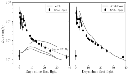
Figure 17: The bolometric light curve of SN2018gep compared to (left) other Ic-BL SNe from the literature (Cano, 2013) and (right) to AT2018cow (Perley et al., 2019a). The dotted line shows the expected contribution from the radioactive decay of $\rm{}^{56}Ni$, for a gamma-ray escape time of 30 $\rm day$ and $M_{\rm Ni}$=0.28 $M_{\odot}$. In order of decreasing $L_{\mathrm{bol}}$, the three Ic-BL SNe are SN1998bw, SN2010bh, and SN2006aj.

The right panel of Figure 17 shows the light curve of SN2018gep compared to that of AT2018cow (Perley et al., 2019a). To estimate the nickel mass of AT2018cow, Perley et al. (2019a) compared the bolometric luminosity at $t\sim 20\,\mbox{$\rm day$}$ to that of SN2002ap (whose nickel mass was derived via late-time nebular spectroscopy; Foley et al. 2003) and found $\mbox{$M_{\rm Ni}$}<0.05\,\mbox{$M_{\odot}$}$. On this scale, we would expect $\mbox{$M_{\rm Ni}$}\lesssim 0.05\,\mbox{$M_{\odot}$}$ for SN2018gep as well.

Finally, Katz et al. (2013) and Wygoda et al. (2019) present an analytical technique for testing whether a light curve is powered by radioactive decay. At late times, the bolometric luminosity is equal to the rate of energy deposition by radioactive decay $Q(t)$, because the diffusion time is much shorter than the dynamical time: $\mbox{$L_{\mathrm{bol}}$}(t)=Q(t)$. At any given time, the energy deposition rate $Q(t)$ is

$$Q(t)=Q_{\gamma}(t)\left(1-e^{-(t_{0}/t)^{2}}\right)+Q_{\mathrm{pos}}(t)$$ (1)

where $Q_{\gamma}(t)$ is the energy release rate of gamma-rays and $t_{0}$ is the time at which the ejecta becomes optically thin to gamma rays. The expression for $Q_{\gamma}(t)$ is

$$\frac{Q_{\gamma}(t)}{10^{43}\,\mbox{$\rm erg$}\,\mbox{$\rm s^{-1}$}}=\frac{\mbox{$M_{\rm Ni}$}}{\mbox{$M_{\odot}$}}\left(6.45e^{-t/8.76\,\mathrm{d}}+1.38e^{-t/111.4\,\mathrm{d}}\right).$$ (2)

$Q_{\mathrm{pos}}(t)$ is the energy deposition rate of positron kinetic energy, and the expression is

$$\frac{Q_{\mathrm{pos}}(t)}{10^{41}\,\mbox{$\rm erg$}\,\mbox{$\rm s^{-1}$}}=4.64\frac{\mbox{$M_{\rm Ni}$}}{\mbox{$M_{\odot}$}}\left(-e^{-t/8.76\,\mathrm{d}}+e^{-t/111.4\,\mathrm{d}}\right).$$ (3)

The dotted line in Figure 17 shows a model track with $\mbox{$M_{\rm Ni}$}=0.28\,M_{\odot}$ and $t_{0}=30\,\mbox{$\rm day$}$. Lower nickel masses produce tracks that are too low to reproduce the data, and larger values of $t_{0}$ produce tracks that drop off too rapidly. Thus on this scale it seems that $\mbox{$M_{\rm Ni}$}\sim 0.3\,\mbox{$M_{\odot}$}$, similar to other Ic-BL SNe (Lyman et al., 2016). Because the data have not yet converged to model tracks, we cannot solve directly for $t_{0}$ and $M_{\rm Ni}$ using the technique for Ia SNe in Wygoda et al. (2019).

We can also try to solve directly for $t_{0}$ and $M_{\rm Ni}$ using the technique for Ia SNe in Wygoda et al. (2019). The first step is to solve for $t_{0}$ using Equation 1 and a second equation resulting from the fact that the expansion is adiabatic,

$$\int_{0}^{t}Q(t^{\prime})\,t^{\prime}\,dt^{\prime}=\int_{0}^{t}L_{\mathrm{bol}}(t^{\prime})\,t^{\prime}\,dt^{\prime}.$$ (4)

The ratio of Equation 1 to Equation 4 removes the dependence on $M_{\rm Ni}$, and enables $t_{0}$ to be measured. However, as shown in Figure 18, the data have not yet converged to model tracks.

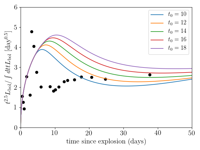
Figure 18: To test whether a light curve is powered by radioactive decay, the ratio of the bolometric luminosity to the time-weighted integrated bolometric luminosity should converge to model tracks, as described in Katz et al. (2013) and Wygoda et al. (2019). This enables a direct measurement of the gamma-ray escape time $t_{0}$ and the nickel mass $M_{\rm Ni}$. However, our data have not converged to these tracks, suggesting that either radioactive decay is not dominant, or that we are not yet in a phase where we can perform this measurement.

4.2 Interaction with extended material

One way to power a rapid and luminous light curve is to deposit energy into circumstellar material (CSM) at large radii (Nakar & Sari, 2010; Nakar & Piro, 2014; Piro, 2015). Since this is a Ic-BL SN, we expect the progenitor to be stripped of its envelope and therefore compact ($R\sim 0.5\,R_{\odot}\sim 10^{10}\,\mbox{$\rm cm$}$; Groh et al. 2013), although there have never been any direct progenitor detections for a Ic-BL SN.

With this expectation, extended material at larger radii would have to arise from mass-loss. This would not be surprising, as massive stars are known to shed a significant fraction of their mass in winds and eruptive episodes; see Smith (2014) for a review.

First we perform an order-of-magnitude calculation to see whether the rise time and peak luminosity could be explained by a model in which shock interaction powers the light curve (“wind shock breakout”). Assuming that the progenitor ejected material with a velocity $v_{w}$ at a time $t$ prior to explosion, the radius of this material at any given time is

$$\begin{split}R_{\mathrm{sh}}&=R_{*}+v_{\mathrm{w}}t\\ &\approx(8.64\times 10^{12}\,\mbox{$\rm cm$})\left(\frac{v_{w}}{1000\,\mbox{$\rm km$}\,\mbox{$\rm s^{-1}$}}\right)\left(\frac{t}{\mbox{$\rm day$}}\right).\end{split}$$ (5)

For material ejected 15 days prior to explosion, traveling at 1000 $\rm km$ $\rm s^{-1}$, the radius would be $R_{\mathrm{CSM}}\sim 10^{14}\,\mbox{$\rm cm$}$ at the time of explosion. The shock crossing timescale is $t_{\mathrm{cross}}$:

$$t_{\mathrm{cross}}\sim R_{\mathrm{CSM}}/v_{s}\approx(0.4\,\mbox{$\rm day$})\left(\frac{R}{10^{14}\,\mbox{$\rm cm$}}\right)\left(\frac{v_{s}}{0.1c}\right)^{-1}$$ (6)

where $v_{s}$ is the velocity of the shock. The shock heats the CSM with an energy density that is roughly half of the kinetic energy of the shock, so $e_{s}\sim(1/2)(\rho v_{s}^{2}/2)$. The luminosity is the total energy deposited divided by $t_{\mathrm{cross}}$,

$$\begin{split}L_{\mathrm{BO}}&\sim\frac{E_{\mathrm{BO}}}{t_{\mathrm{cross}}}\sim\frac{v_{s}^{3}}{4}\frac{dM}{dR}\\ &=(8\times 10^{44}\,\mbox{$\rm erg$}\,\mbox{$\rm s^{-1}$})\left(\frac{v_{s}}{0.1c}\right)^{3}\left(\frac{dM}{\mbox{$M_{\odot}$}}\right)\left(\frac{dR}{10^{14}\,\mbox{$\rm cm$}}\right)^{-1}\end{split}$$ (7)

assuming a constant density. Thus, for shock velocities on the order of the observed photospheric radius expansion ($0.1c$), and a CSM radius on the order of the first photospheric radius that we measure ($3\times 10^{14}\,\mbox{$\rm cm$}$), it is easy to explain the rise time and peak luminosity that we observe.

To test whether shock breakout (and subsequent post-shock cooling) can explain the evolution of the physical properties we measured in Section 3, we ran one-dimensional numerical radiation hydrodynamics simulations of a SN running into a circumstellar shell with CASTRO (Almgren et al., 2010; Zhang et al., 2011). We assume spherical symmetry and solve the coupled equations of radiation hydrodynamics using a grey flux-limited non-equilibrium diffusion approximation. The setup is similar to the models presented in Rest et al. (2018) but with parameters modified to fit SN2018gep.

The ejecta is assumed to be homologously expanding, characterized by a broken power-law density profile, an ejecta mass $M_{\rm ej}$, and energy $E_{\rm ej}$. The ejecta density profile has an inner power-law index of $n=0$ (that is, $\rho(r)\propto r^{-n}$) then steepens to an index $n=10$, as is appropriate for core-collapse SN explosions (Matzner & McKee, 1999). The circumstellar shell is assumed to be uniform in density with radius $R_{\rm CSM}$ and mass $M_{\rm CSM}$. We adopt a uniform opacity of $\kappa=0.2$ cm² g^-1, which is characteristic of hydrogen-poor electron scattering.

The best-fit model, shown in Figure 19, used the following parameters: $M_{\mathrm{ej}}=8\,\mbox{$M_{\odot}$}$, $E_{\mathrm{ej}}=2\times 10^{52}\,\mbox{$\rm erg$}$, $M_{\mathrm{CSM}}=0.02\,\mbox{$M_{\odot}$}$, and $R_{\mathrm{CSM}}=3\times 10^{14}\,\mbox{$\rm cm$}$. The inferred kinetic energy is consistent with typical values measured for Ic-BL SNe (e.g. Cano et al. 2017; Taddia et al. 2019), and $R_{\mathrm{CSM}}$ is similar in value to the first photospheric radius we measure (at $\Delta t=0.05\,\mbox{$\rm day$}$; see Figure 9).

The inferred values presented here are likely uncertain to within a factor of a few, given the degeneracies of the rise time and peak luminosity with the CSM mass and radius. Qualitatively, a larger CSM radius will result in a higher peak luminosity and longer rise time. The peak luminosity is relatively independent of the CSM mass, which instead affects the photospheric velocity and temperature (i.e. a larger CSM mass slows down the post-interaction velocity to a greater extent and increases the shock-heated temperature). A full discussion of the dependencies of the light curve and photospheric properties on the CSM parameters will be presented in an upcoming work (Khatami, D. et al., in preparation).

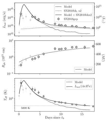
Figure 19: Best-fit CSM interaction model with the light curve of the Ic-BL SN 2010bh (Cano, 2013) scaled up by a factor of two. The model parameters are $M_{\mathrm{ej}}=8\,\mbox{$M_{\odot}$}$, $E_{\mathrm{ej}}=2\times 10^{52}\,\mbox{$\rm erg$}$, $M_{\mathrm{CSM}}=0.02\,\mbox{$M_{\odot}$}$, and $R_{\mathrm{CSM}}=3\times 10^{14}\,\mbox{$\rm cm$}$. As in Figure 9, the outlined circles are derived from UV and optical data, while the light grey circles are derived from optical data only.

In this framework, the shockwave sweeps through the CSM prior to peak luminosity, so that at maximum luminosity the outer parts of the CSM have been swept into a dense shell moving at SN-like velocities ($v_{\mathrm{post-shock}}\approx 3v_{s}/4$). This scenario was laid out in Chevalier & Irwin (2011) and discussed in Kasen (2017). This explains the high velocities we measure at early times and the absence of narrow emission features in our spectra. For another discussion of the absence of narrow emission lines due to an abrupt cutoff in CSM density, see Moriya & Tominaga (2012). Following Chevalier & Irwin (2011), the rapid rise corresponds to shock breakout from the CSM, and begins at a time $R_{\mathrm{CSM}}/v_{\mathrm{sh}}$ after the explosion, where $v_{\mathrm{sh}}$ is the velocity of the shock. The time to peak luminosity (1.2 $\rm day$) is longer than this delay time by a factor ($R_{w}/R_{d}$). Given the best-fit $R_{w}=3\times 10^{14}\,\mbox{$\rm cm$}$, and assuming $R_{d}\sim R_{w}$, we find $v_{\mathrm{sh}}=0.1c$, and an explosion time $\sim 1\,\mbox{$\rm day$}$ prior to $t_{0}$. This model also predicts an increasing temperature while the shock breaks out (i.e. during the rise to peak bolometric luminosity).

Other Ic SNe have shown early evidence for interaction in their light curves, but in other cases the emission has been attributed to post-shock cooling in expanding material rather than shock breakout itself. For example, the first peak observed in iPTF14gqr (De et al., 2018) was short-lived ($\lesssim 2\,\mbox{$\rm day$}$) and attributed to shock-cooling emission from material stripped by a compact companion. iPTF14gqr is different in a number of ways from SN2018gep: the spectra showed high-ionization emission lines, including He II, and the explosion had a much smaller kinetic energy ($E_{K}\approx 10^{50}\,\mbox{$\rm erg$}$) and smaller velocities (10,000 $\rm km$ $\rm s^{-1}$). The main peak in iPTF16asu was also modeled as shock-cooling emission rather than shock breakout (Whitesides et al., 2017).

Under the assumption that the light curve represented post-shock cooling emission, De et al. (2018) and Whitesides et al. (2017) both used one-zone analytic models from Piro (2015) to estimate the properties of the explosion and the CSM. This approximation assumes that the emitting region is a uniformly heated expanding sphere. In iPTF14gqr the inferred properties of the extended material were $M_{e}\sim 8\times 10^{-3}\,M_{\odot}$ at $R_{e}\sim 3\times 10^{13}\,\mbox{$\rm cm$}$. In iPTF16asu the inferred properties of the extended material were $M_{e}\sim 0.45\,M_{\odot}$ at $R_{e}\sim 1.7\times 10^{12}\,\mbox{$\rm cm$}$. The fit also required a more energetic explosion than iPTF14gqr ($4\times 10^{51}\,\mbox{$\rm erg$}$). By applying the same framework to the decline of the bolometric light curve of SN2018gep, we arrive at similar values to those inferred for iPTF16asu, as shown in Figure 20.

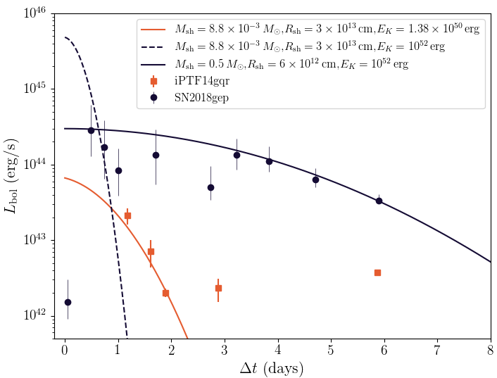
Figure 20: Estimated CSM and explosion properties using models from Piro (2015). The shell mass is much larger than the one in iPTF14gqr, which is the reason for the more extended shock-cooling peak.

We model the main peak of SN2018gep as shock breakout rather than post-shock cooling emission. Our motivation for this choice is that the timescale over which we detect the precursor emission is more consistent with a large radius and lower shell mass. From the shell mass and radius, we can also estimate the mass-loss rate immediately prior to explosion,

$$\frac{\dot{M}}{\mbox{$M_{\odot}$}\,\mbox{$\rm yr^{-1}$}}\approx 32\left(\frac{M_{\mathrm{sh}}}{\mbox{$M_{\odot}$}}\right)\left(\frac{v_{w}}{1000\mbox{$\rm km$}\,\mbox{$\rm s^{-1}$}}\right)\left(\frac{R_{\mathrm{sh}}}{10^{14}\mbox{$\rm cm$}}\right)^{-1}.$$ (8)

For our best-fit parameters $M_{\mathrm{sh}}=0.02\,M_{\odot}$ and $R_{\mathrm{sh}}=3\times 10^{14}\,\mbox{$\rm cm$}$, and taking $v_{w}=1000\,\mbox{$\rm km$}\,\mbox{$\rm s^{-1}$}$, we find $\dot{M}\approx 0.6\,\mbox{$M_{\odot}$}\,\mbox{$\rm yr^{-1}$}$, 4–6 orders of magnitude higher than what is typically expected for Ic-BL SNe (Smith, 2014).

In the shock breakout model, the shock sweeps through confined CSM and passes into lower-density material. Thus, it is not surprising that we do not observe the X-ray or radio emission that would indicate interaction with high-density material. From our VLA observations of SN2018gep, the radio flux marginally decreased from $\Delta t=5\,\mbox{$\rm day$}$ to $\Delta t=75\,\mbox{$\rm day$}$. This could be astrophysical, but could also be instrumental (change in beamsize due to change in VLA configuration). Using the relation of Murphy et al. (2011), the estimated contribution from the host galaxy (for a SFR of $0.12^{+0.08}_{-0.05}\,\mbox{$M_{\odot}$}\,\mbox{$\rm yr^{-1}$}$; see Section 3.3) is

$$\begin{split}\left(\frac{L_{\mathrm{1.4\,\mathrm{GHz}}}}{\mbox{$\rm erg$}\,\mbox{$\rm s^{-1}$}\,\mbox{$\rm Hz^{-1}$}}\right)&\approx 1.57\times 10^{28}\left(\frac{\mathrm{SFR}_{\mathrm{radio}}}{\mbox{$M_{\odot}$}\,\mbox{$\rm yr^{-1}$}}\right)\\ &\approx 1.9\times 10^{27}\,\mbox{$\rm erg$}\,\mbox{$\rm s^{-1}$}\,\mbox{$\rm Hz^{-1}$}.\end{split}$$ (9)

Taking a spectral index of $-0.7$ (a synchrotron spectrum), the expected 9 $\rm GHz$ luminosity would be between $3.0\times 10^{26}\,\mbox{$\rm erg$}\,\mbox{$\rm s^{-1}$}\,\mbox{$\rm Hz^{-1}$}$ and $8.6\times 10^{26}\,\mbox{$\rm erg$}\,\mbox{$\rm s^{-1}$}\,\mbox{$\rm Hz^{-1}$}$. From Table 2, the measured spectral luminosity is $8.3\times 10^{26}\,\mbox{$\rm erg$}\,\mbox{$\rm s^{-1}$}\,\mbox{$\rm Hz^{-1}$}$ (at 10 $\rm GHz$) in the first epoch, and $6\times 10^{26}\,\mbox{$\rm erg$}\,\mbox{$\rm s^{-1}$}\,\mbox{$\rm Hz^{-1}$}$ (at 9 $\rm GHz$) in the second epoch. The slit covering fraction of our LRIS observations is again relevant here; as discussed in Section 3.3, the true SFR is likely a factor of a few higher than what we inferred from modeling the galaxy SED. So, it is plausible that the first two radio detections are entirely due to the host galaxy.

In the third epoch, the luminosity is (at 9 $\rm GHz$) is $<3.9\times 10^{26}\,\mbox{$\rm erg$}\,\mbox{$\rm s^{-1}$}\,\mbox{$\rm Hz^{-1}$}$, although the difference from the first two epochs may be due to the different array configuration. Taking the peak of the 9–10 $\rm GHz$ light curve to be $8.3\times 10^{26}\,\mbox{$\rm erg$}\,\mbox{$\rm s^{-1}$}\,\mbox{$\rm Hz^{-1}$}$ at $\Delta t\approx 5\,\mbox{$\rm day$}$, Figure 21 shows that SN2018gep would be an order of magnitude less luminous in radio emission than any other Ic-BL SN. If the luminosity truly decreased, then the implied mass-loss rate is $\dot{M}\sim 3\times 10^{-6}$, consistent with the idea that the shock has passed from confined CSM into much lower-density material.

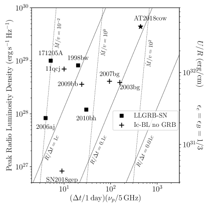
Figure 21: The radio luminosity of SN2018gep compared to AT2018cow and radio-loud Ic-BL SNe (assuming $\epsilon_{e}=\epsilon_{B}=1/3$, cf. Chevalier 1998; Soderberg et al. 2010; Ho et al. 2019). Lines of constant mass-loss rate (scaled to wind velocity) are shown in units of $10^{-4}\,M_{\odot}\,\mbox{$\rm yr^{-1}$}/1000\,\mbox{$\rm km$}\,\mbox{$\rm s^{-1}$}$. The radio luminosity for GRB 171205A was taken from VLA observations reported by Laskar et al. (2017), but we note that this is a lower limit in luminosity and in peak frequency because the source was heavily self-absorbed at this epoch.

If the emission is constant and due entirely to the host galaxy, the point shown in Figure 21 is an upper limit in luminosity. Assuming that the peak of the SED of any radio emission from the SN is not substantially different from the frequencies we measure (i.e. that the spectrum is not self-absorbed at these frequencies), we have a limit on the 9 $\rm GHz$ radio luminosity of $L_{p}\lesssim 10^{27}\,\mbox{$\rm erg$}\,\mbox{$\rm s^{-1}$}\,\mbox{$\rm Hz^{-1}$}$ at $\Delta t\approx 5$–15 $\rm day$.

The shell mass and radius also give an estimate of the optical depth: $\tau\approx\kappa M/r^{2}\approx 100>>1$, which means that the shell would be optically thick. The lack of detected X-ray emission is consistent with the expectation that any X-ray photons produced in the collision would be thermalized by the shell and reradiated as blackbody emission.

Finally, assuming that the rapid rise to peak is indeed caused by shock breakout, we examine whether our model is consistent with our detections in the weeks prior to explosion. Material ejected 10 days prior to the explosion at the escape velocity of a Wolf-Rayet star ($v_{\mathrm{esc}}\sim 1000\,\mbox{$\rm km$}\,\mbox{$\rm s^{-1}$}$) would lie at $R\sim 10^{14}\,\mbox{$\rm cm$}$, which is consistent with our model. Assuming that the emission mechanism is internal shocks between shells of ejected material traveling at different velocities, we can estimate the amount of mass required:

$$\frac{1}{2}\epsilon Mv^{2}=L\tau$$ (10)

where $v\approx 1000\,\mbox{$\rm km$}\,\mbox{$\rm s^{-1}$}$, $\epsilon\approx 0.5$ is the efficiency of thermalizing the kinetic energy of the shells, $M$ is the shell mass, $L\approx 10^{39}\,\mbox{$\rm erg$}\,\mbox{$\rm s^{-1}$}$ is the luminosity we observe, and $\tau\approx 10\,\mbox{$\rm day$}$ is the timescale over which we observe the emission. We find $M\approx 0.02\,\mbox{$M_{\odot}$}$, again consistent with our model.

We conclude that the data are consistent with a scenario in which a compact Ic-BL progenitor underwent a period of eruptive mass-loss shortly prior to explosion. In the terminal explosion, the light curve was initially dominated by shock breakout through (and post-shock cooling of) this recently-ejected material.

Finally, we return to the question of the emission detected in the first few minutes, which showed an inflection point prior to the rapid rise to peak (Figure 2). Given the pre-explosion activity and inference of CSM interaction, it is not surprising that the rise is not well-modeled by a simple quadratic function. One possibility is that we are seeing ejecta already heated from earlier precursor activity. Another possibility is that we are seeing the effects of a finite light travel time. For a sphere of $R\sim 3\times 10^{14}\,\mbox{$\rm cm$}$, the light crossing time is $\sim 20$ minutes. The slower rising phase could represent the time for photons to reach us across the extent of the emitting sphere.

In Table 4, we summarize the key properties inferred from Section 4.

Table 4: Key model properties of SN2018gep

Parameter	Value	Notes
$t_{\rm rise}$	1.2 $\rm day$
$E_{\mathrm{SN}}$	$2\times 10^{52}\,\mbox{$\rm erg$}$
$M_{\rm ej}$	8 $M_{\odot}$
$M_{\mathrm{CSM}}$	0.02 $M_{\odot}$
$R_{\mathrm{CSM}}$	$3\times 10^{14}\,\mbox{$\rm cm$}$
$\dot{M}$	$0.6\,\mbox{$M_{\odot}$}\,\mbox{$\rm yr^{-1}$}$	Assuming $v_{w}=1000\,\mbox{$\rm km$}\,\mbox{$\rm s^{-1}$}$
$M_{\rm Ni}$	$<0.2$–0.3 $M_{\odot}$

5 Comparison to unclassified rapidly evolving transients at high redshift

In terms of the timescale of its light curve evolution, SN2018gep is similar to AT2018cow in fulfilling the criteria that optical surveys use to identify rapidly evolving transients (e.g. Drout et al. 2014; Tanaka et al. 2016; Pursiainen et al. 2018). However, there are a number of ways in which SN2018gep is more of a “typical” member of these populations than AT2018cow. In particular, SN2018gep has an expanding photospheric radius and declining effective temperature. By contrast, one of the challenges in explaining AT2018cow as a stellar explosion was its nearly constant temperature (persistent blue color) and declining photospheric radius. In Figure 22 we show these two different kinds of evolution as very different tracks in color-magnitude space. We also show a late-time point for KSN2015K (Rest et al., 2018), which shows blue colors even after the transient had faded to half-max. The mass-loss rate inferred for Rest et al. (2018) was $2\times 10^{-3}\,\mbox{$M_{\odot}$}\,\mbox{$\rm yr^{-1}$}$.

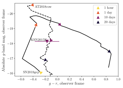
Figure 22: A “color-magnitude” diagram of AT2018cow and SN2018gep, showing the evolution of color with time from first light ($t_{0}$). Like AT2018cow, the fast transient KSN2015K stayed persistently blue even after it had faded to half-maximum. SN2018gep has more typical SN evolution, reddening with time (cooling in temperature).

Of the PS-1 events, most appear to expand, cool, and redden with time (Drout et al., 2014). That said, there are few co-eval data points in multiple filters, even in the gold sample transients. The transients are also faint; all but one lie at $z>0.1$. Of the DES sample, most also show evidence for declining temperatures and increasing radii, although three show evidence of a constant temperature and decreasing radius: 15X3mxf, 16X1eho, and 15C3opk. The peak bolometric luminosities for these three transients are reported as $3\times 10^{43}\,\mbox{$\rm erg$}\,\mbox{$\rm s^{-1}$}$, $9\times 10^{43}\,\mbox{$\rm erg$}\,\mbox{$\rm s^{-1}$}$, and $5\times 10^{43}\,\mbox{$\rm erg$}\,\mbox{$\rm s^{-1}$}$, respectively (Pursiainen et al., 2018).

To estimate a rate of Ic-BL SNe that have a light curve powered by shock breakout, we used the sample of 25 nearby ($z<0.1$) Ic-BL SNe from PTF (Taddia et al., 2019), because these were found in an untargeted survey. Of these, we could not draw a conclusion about eight (either because the peak was not resolved or there was no multi-color photometry available around peak, or both). The remaining clearly lacked the rise time or blue colors of SN2018gep. Furthermore, SN2018gep is unique among the sample of 12 nearby ($z<0.1$) Ic-BL SNe from ZTF discovered so far, which will be presented in a separate publication. From this, we estimate that the rate of Ic-BL SNe with a main peak dominated by shock breakout is no more than 10% of the rate of Ic-BL SNe.

6 Summary and Future Work

In this paper, we presented an unprecedented dataset that connects late-stage eruptive mass loss in a stripped massive star to its subsequent explosion as a rapidly rising luminous transient. Here we summarize our key findings:

1. High-cadence dual-band observations with ZTF (six observations in 3 hours) captured a rapid rise ($1.4\pm 0.1$ mag/hr) to peak luminosity, and a corresponding increase in temperature. This rise rate is second only to that of SN 2016gkg (Bersten et al., 2018), which was attributed to shock breakout in extended material surrounding a Type IIb progenitor. However, the signal in SN2018gep is two magnitudes more luminous.

2. A retrospective search in ZTF data revealed clear detections of precursor emission in the days and months leading up to the terminal explosion. The luminosity of these detections ($M=-14$) and evidence for variability suggests that they arise from eruptive mass-loss, rather than the luminosity of a quiescent progenitor. This is the first definitive pre-explosion detection of a Ic-BL SN to date.

3. The bolometric light curve peaks after a few days at $>3\times 10^{44}\,\mbox{$\rm erg$}\,\mbox{$\rm s^{-1}$}$. At late times, a power-law and an exponential decay are both acceptable fits to the data.

4. The temperature rises to $50,000\,\mbox{$\rm K$}$ in the first day, then declines as $t^{-1}$ then flattens at 5000 K, which we attribute to recombination of carbon and oxygen.

5. The photosphere expands at $v=0.1c$, and flattens once recombination sets in.

6. We obtained nine spectra in the first five days of the explosion, as the effective temperature declined from 50,000 K to 20,000 K. To our knowledge, these represent the earliest-ever spectra of a stripped-envelope SN, in terms of temperature evolution.

7. The early spectra exhibit a “W” feature similar to what has been seen in stripped-envelope superluminous SNe. From a NLTE spectral synthesis model, we find that this can be reproduced with a carbon and oxygen composition.

8. The velocities inferred from the spectra are among the highest observed for stripped-envelope SNe, and are most similar to the velocities of Ic-BL SNe accompanied by GRBs.

9. The host galaxy has a star-formation rate of 0.12 $M_{\odot}$ $\rm yr^{-1}$, and a lower mass and lower metallicity than galaxies hosting GRB-SNe, which are low-mass and low-metallicity compared to the overall core collapse SN population.

10. The early light curve is best-described by shock breakout in extended but confined CSM, with $M=0.02\,\mbox{$M_{\odot}$}$ at $R=3\times 10^{14}\,\mbox{$\rm cm$}$. The implied mass-loss rate is $0.6\,\mbox{$M_{\odot}$}\,\mbox{$\rm yr^{-1}$}$ in the days leading up to the explosion, consistent with our detections of precursor emission. After the initial breakout, the shock runs through CSM of much lower density, hence the lack of narrow emission features and lack of strong radio and X-ray emission.

11. Although SN2018gep is similar to AT2018cow in terms of its bolometric light curve, it has a very different color evolution. In this sense, the “rapidly evolving transients” in the PS-1 and DES samples are more similar to SN2018gep than to AT2018cow.

12. The late-time light curve seems to require an energy deposition mechanism distinct from shock-interaction. Radioactive decay is one possibility, but further monitoring is needed to test this.

The code used to produce the results described in this paper was written in Python and is available online in an open-source repository. When the paper has been accepted for publication, the data will be made publicly available via WISeREP, an interactive repository of supernova data (Yaron & Gal-Yam, 2012).

Here we provide supplementary figures and tables. In Appendix A we provide the full set of optical and UV photometry and the blackbody fits to this photometry. In Appendix B we provide the log of optical and UV spectroscopic observations, as well as a figure showing all of our optical spectra. In Appendix C we include more details about the atomic data used for our spectral modeling. In Appendix D we show the spectrum, line-flux measurements, and photometry that was used to derive properties of the host galaxy.

Appendix A UV and Optical Photometry

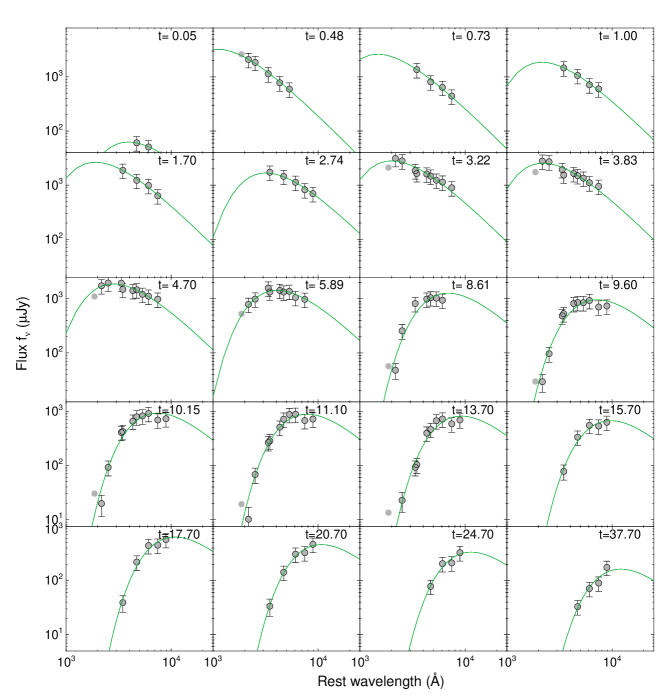
Figure 23: Blackbody fits to Swift/UVOT and optical photometry for SN2018gep. Since the UVOT and ground-based observations were taken at slightly different epochs, we interpolated the data in time using UVOT epochs at early times and LT epochs at later times.

Here we provide our optical and UV photometry (Table 5) and the blackbody fits to this photometry used to derive the photospheric evolution (Figure 23).

Table 5: Optical and ultraviolet photometry for SN2018gep

Date (JD)	$\Delta t$	Instrument	Filter	AB Mag	Error in AB Mag
2458370.6634	0.02	P48+ZTF	r	20.48	0.26
2458370.6856	0.04	P48+ZTF	g	19.70	0.14
2458370.6994	0.05	P48+ZTF	g	19.34	0.11
2458370.7153	0.07	P48+ZTF	g	18.80	0.08
2458370.7612	0.11	P48+ZTF	r	18.36	0.08
2458370.7612	0.11	P48+ZTF	r	18.36	0.08
2458371.6295	0.98	P60+SEDM	r	16.78	0.01
2458371.6323	0.99	P60+SEDM	g	16.39	0.02
2458371.6351	0.99	P60+SEDM	i	17.01	0.01
2458371.6369	0.99	P48+ZTF	r	16.83	0.03
2458371.6378	0.99	P48+ZTF	r	16.81	0.04
2458371.6378	0.99	P48+ZTF	r	16.81	0.04
2458371.6392	0.99	P60+SEDM	u	15.98	0.02
2458371.642	0.99	P60+SEDM	r	16.77	0.01
2458371.6448	1.0	P60+SEDM	g	16.37	0.02
2458371.6476	1.0	P60+SEDM	i	16.97	0.01
2458371.6514	1.0	P48+ZTF	r	16.80	0.03
2458371.6517	1.0	P60+SEDM	u	15.98	0.02
2458371.6838	1.04	P48+ZTF	r	16.78	0.04
2458371.6959	1.05	P48+ZTF	g	16.31	0.02
2458371.6968	1.05	P48+ZTF	g	16.29	0.03
2458371.6968	1.05	P48+ZTF	g	16.29	0.03
2458371.7138	1.07	P48+ZTF	g	16.29	0.03
2458371.7138	1.07	P48+ZTF	g	16.29	0.03
2458371.7359	1.09	P48+ZTF	g	16.28	0.03
2458372.6396	1.99	P48+ZTF	r	16.48	0.04
2458372.6396	1.99	P48+ZTF	r	16.48	0.04
2458372.6586	2.01	P48+ZTF	r	16.49	0.06
2458372.6586	2.01	P48+ZTF	r	16.49	0.06
2458372.6861	2.04	P48+ZTF	r	16.47	0.04
2458372.6861	2.04	P48+ZTF	r	16.47	0.04
2458372.7134	2.07	P48+ZTF	g	15.99	0.03
2458372.7371	2.09	P48+ZTF	g	15.99	0.02
2458372.7371	2.09	P48+ZTF	g	15.99	0.02
2458373.6276	2.98	P48+ZTF	r	16.36	0.03
2458373.6447	3.0	P60+SEDM	r	16.32	0.01
2458373.6464	3.0	P60+SEDM	g	15.99	0.01
2458373.6481	3.0	P60+SEDM	i	16.55	0.01
2458373.6498	3.0	P60+SEDM	u	15.90	0.02
2458373.6627	3.02	P48+ZTF	r	16.35	0.03
2458373.6627	3.02	P48+ZTF	r	16.35	0.03
2458373.685	3.04	P48+ZTF	r	16.34	0.03
2458373.685	3.04	P48+ZTF	r	16.34	0.03
2458373.6984	3.05	P48+ZTF	g	15.91	0.02
2458373.7189	3.07	P48+ZTF	g	15.90	0.03
2458373.736	3.09	P48+ZTF	g	15.91	0.02
2458374.6316	3.98	P48+ZTF	r	16.30	0.04
2458374.6316	3.98	P48+ZTF	r	16.30	0.04
2458374.6429	4.0	P48+ZTF	r	16.32	0.03
2458374.6495	4.0	P48+ZTF	r	16.30	0.03
2458374.6551	4.01	P60+SEDM	r	16.29	0.01
2458374.6569	4.01	P60+SEDM	g	16.03	0.01
2458374.6586	4.01	P60+SEDM	i	16.45	0.01
2458374.6603	4.01	P60+SEDM	u	15.92	0.03
2458374.6845	4.04	P48+ZTF	r	16.29	0.04
2458374.6845	4.04	P48+ZTF	r	16.29	0.04
2458374.6994	4.05	P48+ZTF	g	15.91	0.03
2458374.6994	4.05	P48+ZTF	g	15.91	0.03
2458374.7041	4.06	P48+ZTF	g	15.93	0.02
2458374.7264	4.08	P48+ZTF	g	15.92	0.03
2458374.7428	4.1	P48+ZTF	g	15.91	0.03
2458374.7428	4.1	P48+ZTF	g	15.91	0.03
2458375.6247	4.98	P60+SEDM	r	16.31	0.01
2458375.6265	4.98	P60+SEDM	g	16.07	0.01
2458375.6282	4.98	P60+SEDM	i	16.43	0.01
2458375.6299	4.98	P60+SEDM	u	15.98	0.03
2458375.6757	5.03	P48+ZTF	r	16.33	0.04
2458375.6757	5.03	P48+ZTF	r	16.33	0.04
2458375.7144	5.07	P48+ZTF	g	15.97	0.04
2458375.7144	5.07	P48+ZTF	g	15.97	0.04
2458375.7381	5.09	P48+ZTF	g	15.99	0.03
2458376.62	5.97	P48+ZTF	r	16.37	0.04
2458376.6623	6.02	P60+SEDM	r	16.37	0.01
2458376.6626	6.02	P48+ZTF	r	16.37	0.04
2458376.664	6.02	P60+SEDM	g	16.16	0.02
2458376.6657	6.02	P60+SEDM	i	16.44	0.01
2458376.6674	6.02	P60+SEDM	u	16.09	0.03
2458376.6739	6.03	P48+ZTF	r	16.36	0.04
2458376.7272	6.08	P48+ZTF	g	16.10	0.03
2458376.7272	6.08	P48+ZTF	g	16.10	0.03
2458376.7423	6.1	P48+ZTF	g	16.09	0.03
2458376.7423	6.1	P48+ZTF	g	16.09	0.03
2458377.6186	6.97	P60+SEDM	r	16.40	0.01
2458377.6204	6.97	P60+SEDM	g	16.27	0.02
2458377.6221	6.97	P60+SEDM	i	16.51	0.01
2458377.6238	6.98	P60+SEDM	u	16.29	0.01
2458377.6301	6.98	P48+ZTF	r	16.41	0.03
2458377.6301	6.98	P48+ZTF	r	16.41	0.03
2458377.6513	7.0	P48+ZTF	r	16.41	0.03
2458377.6639	7.02	P48+ZTF	r	16.40	0.03
2458377.6639	7.02	P48+ZTF	r	16.40	0.03
2458377.6761	7.03	P48+ZTF	r	16.41	0.03
2458377.6761	7.03	P48+ZTF	r	16.41	0.03
2458377.6935	7.05	P48+ZTF	g	16.21	0.03
2458377.7038	7.06	P48+ZTF	g	16.20	0.03
2458377.7165	7.07	P48+ZTF	g	16.20	0.04
2458377.7165	7.07	P48+ZTF	g	16.20	0.04
2458377.7458	7.1	P48+ZTF	g	16.22	0.03
2458377.7458	7.1	P48+ZTF	g	16.22	0.03
2458378.6164	7.97	P48+ZTF	r	16.45	0.04
2458378.6437	8.0	P48+ZTF	r	16.46	0.05
2458378.665	8.02	P48+ZTF	g	16.33	0.03
2458378.665	8.02	P48+ZTF	g	16.33	0.03
2458378.6844	8.04	P48+ZTF	g	16.32	0.03
2458378.693	8.05	P60+SEDM	r	16.41	0.01
2458378.7039	8.06	P48+ZTF	g	16.32	0.03
2458378.7158	8.07	P48+ZTF	r	16.47	0.03
2458379.6623	9.02	P48+ZTF	g	16.44	0.04
2458379.6823	9.04	P48+ZTF	g	16.43	0.03
2458379.6823	9.04	P48+ZTF	g	16.43	0.03
2458379.6977	9.05	P48+ZTF	g	16.44	0.03
2458379.7176	9.07	P48+ZTF	r	16.51	0.04
2458379.7409	9.09	P48+ZTF	r	16.52	0.04
2458379.7577	9.11	P48+ZTF	r	16.52	0.03
2458380.6214	9.97	P48+ZTF	g	16.63	0.04
2458380.6251	9.98	P48+ZTF	g	16.66	0.04
2458380.6778	10.03	P48+ZTF	g	16.56	0.03
2458380.6778	10.03	P48+ZTF	g	16.56	0.03
2458381.6238	10.98	P48+ZTF	r	16.58	0.04
2458381.6289	10.98	P48+ZTF	r	16.59	0.04
2458381.659	11.01	P48+ZTF	r	16.59	0.04
2458381.6837	11.04	P48+ZTF	g	16.69	0.04
2458381.7053	11.06	P48+ZTF	g	16.69	0.05
2458381.7122	11.06	P48+ZTF	g	16.71	0.04
2458383.6141	12.97	P48+ZTF	r	16.72	0.05
2458383.6141	12.97	P48+ZTF	r	16.72	0.05
2458383.6342	12.99	P48+ZTF	r	16.68	0.03
2458383.6555	13.01	P48+ZTF	r	16.70	0.04
2458383.6829	13.04	P48+ZTF	g	17.05	0.06
2458383.6829	13.04	P48+ZTF	g	17.05	0.06
2458383.6838	13.04	P48+ZTF	g	17.05	0.04
2458383.6838	13.04	P48+ZTF	g	17.05	0.04
2458383.705	13.06	P48+ZTF	g	17.01	0.05
2458383.7143	13.07	P48+ZTF	g	17.05	0.05
2458383.7143	13.07	P48+ZTF	g	17.05	0.05
2458384.6451	14.0	P48+ZTF	r	16.80	0.05
2458384.6525	14.01	P48+ZTF	r	16.80	0.05
2458384.6741	14.03	P48+ZTF	r	16.80	0.04
2458384.717	14.07	P48+ZTF	g	17.26	0.06
2458384.717	14.07	P48+ZTF	g	17.26	0.06
2458384.7384	14.09	P48+ZTF	g	17.24	0.05
2458385.6151	14.97	P48+ZTF	g	17.45	0.05
2458385.633	14.99	P48+ZTF	g	17.45	0.04
2458385.633	14.99	P48+ZTF	g	17.45	0.04
2458385.6622	15.01	P48+ZTF	g	17.46	0.05
2458385.6622	15.01	P48+ZTF	g	17.46	0.05
2458385.6844	15.04	P48+ZTF	r	16.92	0.04
2458385.6844	15.04	P48+ZTF	r	16.92	0.04
2458385.6919	15.04	P48+ZTF	r	16.92	0.04
2458385.6919	15.04	P48+ZTF	r	16.92	0.04
2458385.7117	15.06	P48+ZTF	r	16.93	0.04
2458385.7117	15.06	P48+ZTF	r	16.93	0.04
2458386.6167	15.97	P48+ZTF	g	17.62	0.07
2458386.6242	15.98	P48+ZTF	g	17.67	0.06
2458386.6242	15.98	P48+ZTF	g	17.67	0.06
2458386.6404	15.99	P48+ZTF	g	17.65	0.06
2458386.6546	16.01	P48+ZTF	g	17.60	0.06
2458386.6994	16.05	P48+ZTF	r	17.02	0.05
2458386.6994	16.05	P48+ZTF	r	17.02	0.04
2458386.7013	16.05	P48+ZTF	r	17.04	0.05
2458386.7158	16.07	P48+ZTF	r	17.04	0.04
2458386.7377	16.09	P48+ZTF	r	17.00	0.05
2458387.6227	16.98	P48+ZTF	r	17.14	0.04
2458387.6227	16.98	P48+ZTF	r	17.14	0.04
2458387.6399	16.99	P48+ZTF	r	17.14	0.05
2458387.6541	17.01	P48+ZTF	r	17.15	0.04
2458387.6541	17.01	P48+ZTF	r	17.15	0.04
2458387.6822	17.03	P48+ZTF	g	17.85	0.08
2458387.6822	17.03	P48+ZTF	g	17.85	0.08
2458387.7041	17.06	P48+ZTF	g	17.83	0.10
2458387.7041	17.06	P48+ZTF	g	17.83	0.10
2458387.7232	17.08	P48+ZTF	g	17.88	0.09
2458387.7232	17.08	P48+ZTF	g	17.88	0.09
2458388.6124	17.97	P60+SEDM	r	17.22	0.02
2458388.6154	17.97	P48+ZTF	g	18.04	0.06
2458388.6154	17.97	P48+ZTF	g	18.04	0.06
2458388.6396	17.99	P48+ZTF	g	17.99	0.07
2458388.6396	17.99	P48+ZTF	g	17.99	0.07
2458388.6542	18.01	P48+ZTF	g	18.04	0.06
2458388.6542	18.01	P48+ZTF	g	18.04	0.06
2458388.6834	18.04	P48+ZTF	r	17.30	0.06
2458388.6936	18.05	P48+ZTF	r	17.30	0.05
2458388.7203	18.07	P48+ZTF	r	17.25	0.06
2458389.6156	18.97	P48+ZTF	r	17.39	0.06
2458389.6227	18.98	P48+ZTF	r	17.40	0.05
2458389.6317	18.98	P48+ZTF	g	18.20	0.06
2458389.6317	18.98	P48+ZTF	g	18.20	0.06
2458389.6416	18.99	P48+ZTF	g	18.20	0.06
2458389.6416	18.99	P48+ZTF	g	18.20	0.06
2458389.6804	19.03	P48+ZTF	g	18.21	0.08
2458389.6804	19.03	P48+ZTF	g	18.21	0.08
2458389.6947	19.05	P48+ZTF	g	18.21	0.09
2458389.6947	19.05	P48+ZTF	g	18.21	0.09
2458389.7166	19.07	P48+ZTF	r	17.41	0.05
2458389.7476	19.1	P48+ZTF	r	17.43	0.04
2458390.6228	19.98	P48+ZTF	g	18.43	0.06
2458390.6228	19.98	P48+ZTF	g	18.43	0.06
2458390.6326	19.99	P48+ZTF	g	18.40	0.06
2458390.6326	19.99	P48+ZTF	g	18.40	0.06
2458390.6797	20.03	P48+ZTF	r	17.55	0.04
2458390.7209	20.07	P48+ZTF	r	17.56	0.07
2458390.7347	20.09	P48+ZTF	r	17.53	0.05
2458399.5989	28.95	P48+ZTF	g	19.40	0.19
2458399.5989	28.95	P48+ZTF	g	19.40	0.19
2458400.6307	29.98	P48+ZTF	g	19.46	0.13
2458400.6638	30.02	P48+ZTF	r	18.68	0.11
2458400.6756	30.03	P48+ZTF	r	18.72	0.10
2458400.6756	30.03	P48+ZTF	r	18.72	0.10
2458400.6987	30.05	P48+ZTF	r	18.65	0.14
2458415.6169	44.97	P60+SEDM	r	19.62	0.10
2458415.6196	44.97	P60+SEDM	g	20.24	0.20
2458415.6223	44.98	P60+SEDM	i	19.39	0.06
2458420.593	49.95	P60+SEDM	r	19.74	0.03
2458420.5958	49.95	P60+SEDM	g	20.74	0.06
2458420.5984	49.95	P60+SEDM	i	19.53	0.03
2458420.6011	49.95	P60+SEDM	r	19.76	0.04
2458420.6038	49.96	P60+SEDM	g	20.90	0.08
2458423.584	52.94	P60+SEDM	r	19.78	0.10
2458423.5894	52.94	P60+SEDM	i	19.67	0.13
2458429.5848	58.94	P60+SEDM	r	20.03	0.06
2458429.5875	58.94	P60+SEDM	g	21.32	0.11
2458429.5902	58.94	P60+SEDM	i	19.80	0.04
2458371.3802	0.73	LT	u	16.06	0.01
2458372.3561	1.71	LT	u	15.70	0.01
2458373.3944	2.75	LT	u	15.79	0.01
2458380.3607	9.71	LT	u	17.12	0.02
2458380.3612	9.71	LT	u	17.12	0.02
2458381.3403	10.69	LT	u	17.49	0.03
2458381.3409	10.69	LT	u	17.59	0.04
2458382.3451	11.7	LT	u	17.97	0.04
2458383.3399	12.69	LT	u	18.27	0.06
2458383.3404	12.69	LT	u	18.27	0.06
2458384.34	13.69	LT	u	18.71	0.08
2458384.3405	13.69	LT	u	18.86	0.10
2458385.339	14.69	LT	u	18.89	0.11
2458386.3369	15.69	LT	u	19.16	0.17
2458388.3375	17.69	LT	u	20.07	0.22
2458388.338	17.69	LT	u	19.91	0.28
2458391.3458	20.7	LT	u	20.08	0.24
2458371.3794	0.73	LT	g	16.64	0.01
2458372.3554	1.71	LT	g	16.21	0.01
2458373.3951	2.75	LT	g	16.03	0.01
2458380.3599	9.71	LT	g	16.63	0.01
2458381.3396	10.69	LT	g	16.74	0.01
2458382.3438	11.7	LT	g	16.88	0.01
2458383.3391	12.69	LT	g	17.04	0.01
2458384.3392	13.69	LT	g	17.27	0.01
2458385.3377	14.69	LT	g	17.49	0.01
2458386.3362	15.69	LT	g	17.62	0.05
2458388.3367	17.69	LT	g	18.08	0.01
2458389.3394	18.69	LT	g	18.20	0.01
2458390.367	19.72	LT	g	18.34	0.06
2458391.3445	20.7	LT	g	18.55	0.01
2458393.3452	22.7	LT	g	18.88	0.02
2458394.3463	23.7	LT	g	18.96	0.01
2458395.3462	24.7	LT	g	19.20	0.03
2458396.3496	25.7	LT	g	19.31	0.03
2458397.3884	26.74	LT	g	19.53	0.04
2458407.3531	36.71	LT	g	20.08	0.06
2458407.3537	36.71	LT	g	20.24	0.07
2458408.3179	37.67	LT	g	20.26	0.10
2458408.3186	37.67	LT	g	20.14	0.07
2458409.3255	38.68	LT	g	20.15	0.09
2458409.3262	38.68	LT	g	20.34	0.12
2458371.3787	0.73	LT	r	16.89	0.01
2458372.3546	1.71	LT	r	16.43	0.01
2458373.3958	2.75	LT	r	16.28	0.01
2458380.3592	9.71	LT	r	16.51	0.01
2458381.3389	10.69	LT	r	16.54	0.01
2458382.3431	11.7	LT	r	16.60	0.01
2458383.3384	12.69	LT	r	16.68	0.01
2458384.3385	13.69	LT	r	16.78	0.01
2458385.337	14.69	LT	r	16.91	0.01
2458386.3354	15.69	LT	r	17.07	0.01
2458388.336	17.69	LT	r	17.31	0.01
2458389.3387	18.69	LT	r	17.40	0.01
2458390.3663	19.72	LT	r	17.59	0.04
2458391.3438	20.7	LT	r	17.70	0.01
2458393.3444	22.7	LT	r	17.93	0.01
2458394.3456	23.7	LT	r	18.07	0.01
2458395.3455	24.7	LT	r	18.14	0.02
2458396.3489	25.7	LT	r	18.31	0.02
2458397.3877	26.74	LT	r	18.41	0.02
2458407.3524	36.71	LT	r	19.20	0.03
2458408.317	37.67	LT	r	19.29	0.04
2458409.3246	38.68	LT	r	19.41	0.16
2458371.378	0.73	LT	i	17.30	0.01
2458372.3539	1.71	LT	i	16.90	0.01
2458373.3965	2.75	LT	i	16.62	0.01
2458380.3585	9.71	LT	i	16.81	0.01
2458381.3381	10.69	LT	i	16.82	0.01
2458382.3424	11.7	LT	i	16.88	0.01
2458383.3377	12.69	LT	i	16.92	0.01
2458384.3378	13.69	LT	i	16.99	0.17
2458385.3363	14.69	LT	i	17.04	0.01
2458386.3347	15.69	LT	i	17.10	0.01
2458388.3353	17.69	LT	i	17.28	0.01
2458389.338	18.69	LT	i	17.39	0.01
2458390.3656	19.72	LT	i	17.56	0.04
2458391.3431	20.7	LT	i	17.63	0.01
2458393.3437	22.7	LT	i	17.84	0.01
2458394.3449	23.7	LT	i	17.98	0.01
2458395.3448	24.7	LT	i	18.10	0.04
2458396.3481	25.7	LT	i	18.18	0.01
2458397.3869	26.74	LT	i	18.30	0.02
2458407.3517	36.7	LT	i	19.04	0.03
2458408.3162	37.67	LT	i	19.03	0.07
2458409.3238	38.68	LT	i	19.14	0.07
2458373.3972	2.75	LT	z	16.82	0.01
2458380.3577	9.71	LT	z	16.77	0.01
2458381.3374	10.69	LT	z	16.79	0.01
2458382.3416	11.69	LT	z	16.80	0.01
2458383.3369	12.69	LT	z	16.82	0.01
2458384.337	13.69	LT	z	16.83	0.01
2458385.3355	14.69	LT	z	16.89	0.01
2458386.334	15.69	LT	z	16.94	0.01
2458388.3345	17.69	LT	z	17.04	0.01
2458389.3372	18.69	LT	z	17.11	0.02
2458390.3648	19.72	LT	z	17.23	0.12
2458391.3423	20.7	LT	z	17.26	0.01
2458393.343	22.7	LT	z	17.44	0.01
2458394.3441	23.7	LT	z	17.55	0.02
2458395.344	24.7	LT	z	17.65	0.05
2458396.3474	25.7	LT	z	17.69	0.02
2458397.3862	26.74	LT	z	17.77	0.03
2458407.3509	36.7	LT	z	18.19	0.03
2458408.3155	37.67	LT	z	18.33	0.06
2458409.3231	38.68	LT	z	18.26	0.07
2458374.9769	4.33	LOT	g	16.14	0.01
2458375.9702	5.32	LOT	g	16.17	0.01
2458379.9736	9.33	LOT	g	16.62	0.01
2458381.0023	10.36	LOT	g	16.77	0.01
2458381.9909	11.34	LOT	g	16.89	0.01
2458386.0102	15.36	LOT	g	17.60	0.01
2458391.0243	20.38	LOT	g	18.59	0.01
2458391.9648	21.32	LOT	g	18.72	0.01
2458392.9823	22.34	LOT	g	18.83	0.01
2458393.9679	23.32	LOT	g	18.98	0.01
2458394.9508	24.3	LOT	g	19.16	0.02
2458395.9525	25.31	LOT	g	19.26	0.01
2458396.9584	26.31	LOT	g	19.43	0.02
2458406.9893	36.34	LOT	g	20.32	0.07
2458411.95	41.3	LOT	g	20.53	0.10
2458374.9847	4.34	LOT	i	16.53	0.01
2458379.9812	9.33	LOT	i	16.75	0.01
2458381.01	10.36	LOT	i	16.78	0.01
2458381.9986	11.35	LOT	i	16.80	0.01
2458386.018	15.37	LOT	i	17.05	0.01
2458391.0321	20.38	LOT	i	17.57	0.01
2458391.9726	21.33	LOT	i	17.71	0.01
2458392.9901	22.34	LOT	i	17.80	0.01
2458393.9756	23.33	LOT	i	17.97	0.01
2458394.9692	24.32	LOT	i	18.07	0.01
2458395.9603	25.31	LOT	i	18.16	0.01
2458396.978	26.33	LOT	i	18.25	0.01
2458406.9971	36.35	LOT	i	18.90	0.03
2458411.9578	41.31	LOT	i	19.09	0.04
2458374.9807	4.33	LOT	r	16.30	0.01
2458375.974	5.33	LOT	r	16.33	0.01
2458379.9774	9.33	LOT	r	16.54	0.01
2458381.0061	10.36	LOT	r	16.61	0.01
2458381.9947	11.35	LOT	r	16.62	0.01
2458386.014	15.37	LOT	r	16.97	0.01
2458391.0282	20.38	LOT	r	17.71	0.01
2458391.9686	21.32	LOT	r	17.77	0.01
2458392.9862	22.34	LOT	r	17.93	0.01
2458393.9717	23.32	LOT	r	18.06	0.01
2458394.9653	24.32	LOT	r	18.19	0.01
2458395.9564	25.31	LOT	r	18.30	0.01
2458396.9623	26.31	LOT	r	18.42	0.01
2458406.9932	36.35	LOT	r	19.07	0.02
2458411.9538	41.31	LOT	r	19.42	0.03
2458371.0917	0.44	UVOT	B	16.77	0.06
2458371.1601	0.51	UVOT	B	16.67	0.06
2458373.8837	3.24	UVOT	B	15.88	0.07
2458374.0828	3.44	UVOT	B	15.87	0.08
2458374.481	3.83	UVOT	B	15.90	0.07
2458375.3416	4.69	UVOT	B	16.06	0.06
2458376.48	5.83	UVOT	B	16.00	0.06
2458376.599	5.95	UVOT	B	16.23	0.07
2458379.2575	8.61	UVOT	B	16.46	0.07
2458380.184	9.54	UVOT	B	16.50	0.08
2458380.3172	9.67	UVOT	B	16.68	0.09
2458380.7873	10.14	UVOT	B	16.80	0.07
2458381.6447	11.0	UVOT	B	17.29	0.14
2458381.7774	11.13	UVOT	B	16.80	0.11
2458381.8438	11.2	UVOT	B	16.95	0.12
2458383.3045	12.66	UVOT	B	17.68	0.15
2458383.3705	12.72	UVOT	B	17.35	0.13
2458384.3114	13.66	UVOT	B	17.44	0.08
2458371.0908	0.44	UVOT	U	16.41	0.06
2458371.1591	0.51	UVOT	U	16.24	0.05
2458373.8834	3.24	UVOT	U	15.75	0.07
2458374.0825	3.44	UVOT	U	15.68	0.07
2458374.4806	3.83	UVOT	U	15.76	0.07
2458375.3411	4.69	UVOT	U	15.72	0.06
2458376.4794	5.83	UVOT	U	15.95	0.06
2458376.5986	5.95	UVOT	U	15.83	0.06
2458379.2569	8.61	UVOT	U	16.65	0.07
2458380.1836	9.54	UVOT	U	17.21	0.10
2458380.3168	9.67	UVOT	U	17.28	0.10
2458380.7866	10.14	UVOT	U	17.34	0.08
2458381.6444	11.0	UVOT	U	17.73	0.14
2458381.7771	11.13	UVOT	U	17.94	0.15
2458381.8435	11.2	UVOT	U	18.06	0.17
2458383.3041	12.66	UVOT	U	18.82	0.24
2458383.37	12.72	UVOT	U	18.36	0.17
2458384.3105	13.66	UVOT	U	19.01	0.16
2458371.1013	0.45	UVOT	UVM2	15.74	0.05
2458371.1669	0.52	UVOT	UVM2	15.61	0.05
2458373.8864	3.24	UVOT	UVM2	15.19	0.05
2458374.0856	3.44	UVOT	UVM2	15.19	0.05
2458374.4841	3.84	UVOT	UVM2	15.40	0.05
2458375.3466	4.7	UVOT	UVM2	15.88	0.05
2458376.4854	5.84	UVOT	UVM2	16.66	0.06
2458376.6032	5.96	UVOT	UVM2	16.81	0.06
2458379.2631	8.62	UVOT	UVM2	19.83	0.21
2458380.1881	9.54	UVOT	UVM2	20.14	0.29
2458380.3209	9.67	UVOT	UVM2	20.31	0.35
2458380.7945	10.15	UVOT	UVM2	21.34	0.64
2458381.648	11.0	UVOT	UVM2	21.12	0.67
2458381.7807	11.13	UVOT	UVM2	20.60	0.44
2458381.8472	11.2	UVOT	UVM2	21.87	1.23
2458383.3088	12.66	UVOT	UVM2	21.45	0.81
2458383.3752	12.73	UVOT	UVM2	22.09	1.38
2458384.3213	13.67	UVOT	UVM2	26.70	76.24
2458371.0893	0.44	UVOT	UVW1	15.86	0.05
2458371.1577	0.51	UVOT	UVW1	15.75	0.05
2458373.8829	3.24	UVOT	UVW1	15.32	0.06
2458374.082	3.43	UVOT	UVW1	15.24	0.05
2458374.4801	3.83	UVOT	UVW1	15.42	0.05
2458375.3402	4.69	UVOT	UVW1	15.73	0.05
2458376.4784	5.83	UVOT	UVW1	16.45	0.06
2458376.5979	5.95	UVOT	UVW1	16.50	0.06
2458379.2558	8.61	UVOT	UVW1	17.94	0.09
2458380.1828	9.54	UVOT	UVW1	18.69	0.15
2458380.3161	9.67	UVOT	UVW1	19.08	0.19
2458380.7853	10.14	UVOT	UVW1	18.84	0.13
2458381.6437	11.0	UVOT	UVW1	19.08	0.20
2458381.7765	11.13	UVOT	UVW1	19.41	0.26
2458381.8429	11.2	UVOT	UVW1	20.01	0.39
2458383.3033	12.66	UVOT	UVW1	20.19	0.38
2458383.3692	12.72	UVOT	UVW1	20.72	0.57
2458384.3086	13.66	UVOT	UVW1	20.57	0.35
2458371.0941	0.45	UVOT	UVW2	15.51	0.06
2458371.1625	0.52	UVOT	UVW2	15.38	0.06
2458373.8845	3.24	UVOT	UVW2	15.62	0.06
2458374.0835	3.44	UVOT	UVW2	15.68	0.06
2458374.4818	3.83	UVOT	UVW2	15.88	0.06
2458375.343	4.7	UVOT	UVW2	16.37	0.06
2458376.4815	5.83	UVOT	UVW2	17.09	0.07
2458376.6002	5.95	UVOT	UVW2	17.29	0.08
2458379.2591	8.61	UVOT	UVW2	19.61	0.18
2458380.1852	9.54	UVOT	UVW2	20.11	0.28
2458380.3183	9.67	UVOT	UVW2	20.33	0.34
2458380.7894	10.14	UVOT	UVW2	20.37	0.28
2458381.6457	11.0	UVOT	UVW2	20.23	0.34
2458381.7783	11.13	UVOT	UVW2	20.86	0.56
2458381.8447	11.2	UVOT	UVW2	21.58	1.00
2458383.3057	12.66	UVOT	UVW2	21.53	0.85
2458383.3718	12.72	UVOT	UVW2	21.77	1.00
2458384.3142	13.67	UVOT	UVW2	21.17	0.48
2458371.0965	0.45	UVOT	V	17.25	0.13
2458371.1649	0.52	UVOT	V	16.79	0.10
2458373.8852	3.24	UVOT	V	16.24	0.14
2458374.0843	3.44	UVOT	V	16.13	0.13
2458374.4827	3.84	UVOT	V	16.08	0.12
2458375.3444	4.7	UVOT	V	16.22	0.10
2458376.483	5.84	UVOT	V	16.07	0.09
2458376.6013	5.95	UVOT	V	16.03	0.11
2458379.2607	8.61	UVOT	V	16.41	0.11
2458380.1863	9.54	UVOT	V	16.41	0.13
2458380.3193	9.67	UVOT	V	16.62	0.15
2458380.7914	10.14	UVOT	V	16.62	0.11
2458381.6466	11.0	UVOT	V	16.61	0.16
2458381.7793	11.13	UVOT	V	16.70	0.17
2458381.8456	11.2	UVOT	V	16.51	0.16
2458383.3069	12.66	UVOT	V	16.58	0.14
2458383.3731	12.73	UVOT	V	16.74	0.15
2458384.317	13.67	UVOT	V	16.86	0.11

Appendix B UV and Optical Spectroscopy

The observation log of our UV and optical spectra is provided in Table 6. A plot showing the full sequence of optical spectra is shown in Figure 24.

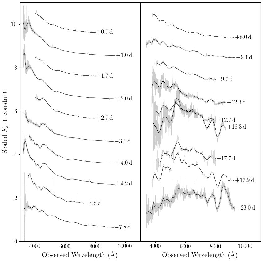
Figure 24: Ground-based optical spectra of SN2018gep. The light grey represents the observed spectrum, interpolating over host emission lines and telluric features. The black line is a Gaussian-smoothed version of the spectrum, using a Gaussian width that is several times the width of a galaxy emission line at that resolution. For more details on the smoothing procedure, see Section 2.1 of Ho et al. (2017).

Table 6: Log of SN2018gep optical spectra

Start Time (UTC)	$\Delta t$	Instrument	Exp. Time (s)	Airmass
2018 Sep 09 20:30:01	0.7	LT+SPRAT	1200	1.107
2018 Sep 10 04:28:51	1.0	P200+DBSP	600	1.283
2018 Sep 10 21:03:42	1.7	LT+SPRAT	900	1.182
2018 Sep 11 04:59:19	2.0	P200+DBSP	600	1.419
2018 Sep 11 20:22:35	2.7	LT+SPRAT	900	1.107
2018 Sep 12 06:09:59	3.1	P200+DBSP
2018 Sep 13 03:52:58	4.0	P200+DBSP	300	1.209
2018 Sep 13 09:17:25	4.2	Keck1+LRIS	300	3.483
2018 Sep 14 02:44:24.24	4.8	DCT+Deveny+LMI	300	1.11
2018 Sep 17 04:38:40	8.0	P60+SEDM	1440	1.435
2018 Sep 17 20:40:25.750	8.7	NOT+ALFOSC	1800	1.19
2018 Sep 18 05:21:58	9.1	P200+DBSP	600	1.720
2018 Sep 18 20:14:35	9.7	LT+SPRAT	1000	1.143
2018 Sep 21 11:15:10	12.3	XLT+BFOSC	3000	1.181
2018 Sep 21 20:58:21	12.7	LT+SPRAT	1000	1.293
2018 Sep 25 11:16:43	16.3	XLT+BFOSC	3000	1.225
2018 Sep 26 20:22:54	17.7	LT+SPRAT	1000	1.242
2018 Sep 27 02:42:29	17.9	P60+SEDM	1440	1.172
2018 Oct 02 04:34:35	23.0	P200+DBSP	600	1.780
2018 Nov 09 05:26:17	61.1	Keck1+LRIS	900	3.242

Note. — Gratings used: Wasatch600 (LT+SPRAT), Gr4 (NOT+ALFOSC), 600/4000 (P200+DBSP; blue side), 316/7500 (P200+DBSP; red side), 400/8500 (Keck1+LRIS; red side).

Filters used: 400nm (LT+SPRAT), open (NOT+ALFOSC), clear (Keck1+LRIS)

Wavelength range: 4020–7995 Å (LT+SPRAT), 3200–9600 Å (NOT+ALFOSC), 1759–10311 Å (Keck1+LRIS), 3777–9223 Å (P60+SEDM)

Resolution: 20 (LT+SPRAT), 710 (NOT+ALFOSC)

Appendix C Atomic data for spectral modeling

The atomic data used for the spectral modelling in Section 3.2 is the same as described in Appendix A.4 of Ergon et al. (2018), but with the following modifications. The stage II-IV ions where (whenever possible) updated to include at least 50 levels for N, Na, Al, Ar and Ca, at least 100 levels for C, O, Ne, Mg, Si and S, and at least 300 levels for Sc, Ti, V, Cr, Mn, Fe, Co and Ni. In addition we updated the C II - C IV and O II - O III ions with specific recombination rates from the online table by S. Nahar.

Appendix D Data for measuring host properties

In this section we provide the data that we used to derive properties of the host galaxy of SN2018gep: the host-galaxy spectrum (Figure 25), line fluxes extracted from this spectrum (Table 7), and host-galaxy photometry (Table 8).

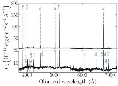
Figure 25: Host spectrum of SN2018gep obtained with Keck/LRIS on 9 November 2018, about two months after explosion. Strong emission lines from the host galaxy are labeled. The low host metallicity of 0.1 solar is reflected by very small N II/H$\alpha$ flux ratio. The large rest-frame [O III]$\lambda$5007 equivalent width of $>160$ Å puts the host also in regime of extreme emission-line galaxies. These galaxy class constitute $<2\%$ of all star-forming galaxies at $z<0.3$ in the SDSS DR15 catalogue. The undulations are due to the supernova. The spectrum is truncated at 7250 Å for presentation purposes, and it is corrected for Galactic reddening.

Table 7: Line fluxes from the host galaxy of SN2018gep extracted from the Keck/LRIS spectrum obtained on 9 November 2018.

Transition	$\lambda_{\rm obs}$	$F$
	(Å)	$\left(10^{-17}~{}{\rm erg\,cm}^{-2}\,{\rm s}^{-1}\right)$
[O II]$\lambda\lambda$3726,3729	$3848.17\pm 0.05$	$334.5\pm 6.23$
[Ne III]$\lambda$3869	$3993.50\pm 0.16$	$82.34\pm 6.18$
He I$\lambda$3889,H-8	$4014.49\pm 0.16$	$29.01\pm 4.73$
[Ne III]$\lambda$3968,H$\epsilon$	$4096.66\pm 0.26$	$36.61\pm 3.98$
H$\delta$	$4233.87\pm 0.13$	$44.88\pm 2.59$
H$\gamma$	$4480.20\pm 0.10$	$81.95\pm 3.74$
[O III]$\lambda$4364	$4503.68\pm 0.10$	$15.01\pm 2.69$
H$\beta$	$5017.87\pm 0.08$	$213.41\pm 10.53$
[O III]$\lambda$4960	$5118.61\pm 0.04$	$352.42\pm 6.50$
[O III]$\lambda$5008	$5168.04\pm 0.04$	$1066.70\pm 19.50$
He I$\lambda$5877	$6064.21\pm 0.20$	$27.04\pm 2.30$
O I$\lambda$6302	$6502.18\pm 1.08$	$6.72\pm 2.94$
[N II]$\lambda$6549	$6758.16\pm 0.02$	$11.15\pm 6.73$
H$\alpha$	$6773.40\pm 0.02$	$723.85\pm 7.65$
[N II]$\lambda$6585	$6794.67\pm 0.02$	$19.01\pm 5.76$
[He I]$\lambda$6678	$6890.29\pm 0.14$	$7.88\pm 2.19$
[S II]$\lambda$6718	$6931.83\pm 0.10$	$41.76\pm 2.38$
[S II]$\lambda$6732	$6946.68\pm 0.10$	$28.15\pm 2.19$

Table 8: Brightness of the host galaxy from UV ot IR wavelenghts

Instrument/	$\lambda_{\rm eff}$	Brightness	Instrument/	$\lambda_{\rm eff}$	Brightness
Filter	(Å)	(mag)	Filter	(Å)	(mag)
GALEX/FUV	1542.3	$20.20\pm 0.03$	SDSS/$i^{\prime}$	7439.5	$18.62\pm 0.04$
GALEX/NUV	2274.4	$20.09\pm 0.03$	SDSS/$z^{\prime}$	8897.1	$18.59\pm 0.12$
UVOT/$w2$	2030.5	$19.91\pm 0.12$	PS1/$g_{\rm PS1}$	4775.6	$18.96\pm 0.04$
UVOT/$m2$	2228.1	$20.00\pm 0.14$	PS1/$r_{\rm PS1}$	6129.5	$18.82\pm 0.04$
UVOT/$w1$	2589.1	$20.11\pm 0.16$	PS1/$i_{\rm PS1}$	7484.6	$18.88\pm 0.04$
UVOT/$u$	3501.2	$19.74\pm 0.16$	PS1/$z_{\rm PS1}$	8657.8	$18.71\pm 0.05$
UVOT/$b$	4328.6	$19.45\pm 0.20$	WIRCam/$J$	12481.5	$18.99\pm 0.09$
UVOT/$v$	5402.1	$18.45\pm 0.21$	2MASS/$H$	16620.0	$18.33\pm 0.36$
SDSS/$u^{\prime}$	3594.9	$19.97\pm 0.12$	WISE/$W1$	33526.0	$19.39\pm 0.08$
SDSS/$g^{\prime}$	4640.4	$18.88\pm 0.02$	WISE/$W2$	46028.0	$19.85\pm 0.19$
SDSS/$r^{\prime}$	6122.3	$18.76\pm 0.05$

References

- Ahn et al. (2014) Ahn, C. P., Alexandroff, R., Allende Prieto, C., et al. 2014, ApJS, 211, 17
- Ahn et al. (2012) Ahn, C. P., Alexandroff, R., Allende Prieto, C., et al. 2012, ApJS, 203, 21.
- Alard, & Lupton (1998) Alard, C., & Lupton, R. H. 1998, ApJ, 503, 325
- Almgren et al. (2010) Almgren, A. S., Beckner, V. E., Bell, J. B., et al. 2010, ApJ, 715, 1221
- Arcavi et al. (2016) Arcavi, I., Wolf, W. M., Howell, D. A., et al. 2016, ApJ, 819, 35
- Arnouts et al. (1999) Arnouts, S., Cristiani, S., Moscardini, L., et al. 1999, MNRAS, 310, 540
- Asplund et al. (2009) Asplund, M., Grevesse, N., Sauval, A. J., & Scott, P. 2009, ARA&A, 47, 481
- Astropy Collaboration et al. (2013) Astropy Collaboration, Robitaille, T. P., Tollerud, E. J., et al. 2013, A&A, 558, A33
- Astropy Collaboration et al. (2018) Astropy Collaboration, Price-Whelan, A. M., Sipőcz, B. M., et al. 2018, AJ, 156, 123
- Barbary et al. (2016) Barbary, K. 2016, extinction, v0.3.0, Zenodo, doi: 10.5281/zenodo.804967, https://github.com/kbarbary/extinction
- Barthelmy et al. (2005) Barthelmy, S. D., Barbier, L. M., Cummings, J. R., et al. 2005, Space Sci. Rev., 120, 143
- Becker (2015) Becker, A. 2015, HOTPANTS: High Order Transform of PSF ANd Template Subtraction, ascl:1504.004
- Bellm et al. (2019a) Bellm, E. C., Kulkarni, S. R., Graham, M. J., et al. 2019, PASP, 131, 018002
- Bellm et al. (2019) Bellm, E. C., Kulkarni, S. R., Barlow, T., et al. 2019, PASP, 131, 068003
- Ben-Ami et al. (2012) Ben-Ami, S., Gal-Yam, A., Filippenko, A. V., et al. 2012, ApJ, 760, L33
- Bersier et al. (2006) Bersier, D., Fruchter, A. S., Strolger, L.-G., et al. 2006, ApJ, 643, 284
- Bersten et al. (2018) Bersten, M. C., Folatelli, G., García, F., et al. 2018, Nature, 554, 497
- Bertin (2010) Bertin, E. 2010, SWarp: Resampling and Co-adding FITS Images Together, ascl:1010.068
- Narayana Bhat et al. (2016) Narayana Bhat, P., Meegan, C. A., von Kienlin, A., et al. 2016, The Astrophysical Journal Supplement Series, 223, 28.
- Blackburn et al. (2015) Blackburn, L., Briggs, M. S., Camp, J., et al. 2015, The Astrophysical Journal Supplement Series, 217, 8.
- Blagorodnova et al. (2018) Blagorodnova, N., Neill, J. D., Walters, R., et al. 2018, PASP, 130, 035003
- Blanton, & Roweis (2007) Blanton, M. R., & Roweis, S. 2007, AJ, 133, 734
- Blaufuss (2018) Blaufuss, E. 2018, The Astronomer’s Telegram, 12062,
- Bourne et al. (2012) Bourne, N., Maddox, S. J., Dunne, L., et al. 2012, MNRAS, 421, 3027
- Branch et al. (2002) Branch, D., Benetti, S., Kasen, D., et al. 2002, ApJ, 566, 1005
- Breeveld et al. (2011) Breeveld, A. A., Landsman, W., Holland, S. T., et al. 2011, American Institute of Physics Conference Series, 373
- Bruzual & Charlot (2003) Bruzual, G., & Charlot, S. 2003, MNRAS, 344, 1000
- Bufano et al. (2012) Bufano, F., Pian, E., Sollerman, J., et al. 2012, ApJ, 753, 67
- Calzetti et al. (2000) Calzetti, D., Armus, L., Bohlin, R. C., et al. 2000, ApJ, 533, 682
- Campana et al. (2006) Campana, S., Mangano, V., Blustin, A. J., et al. 2006, Nature, 442, 1008
- Cano (2013) Cano, Z. 2013, MNRAS, 434, 1098
- Cano et al. (2017) Cano, Z., Wang, S.-Q., Dai, Z.-G., & Wu, X.-F. 2017, Advances in Astronomy, 2017, 8929054
- Cano et al. (2017) Cano, Z., Izzo, L., de Ugarte Postigo, A., et al. 2017, A&A, 605, A107
- Cenko et al. (2006) Cenko, S. B., Fox, D. B., Moon, D.-S., et al. 2006, PASP, 118, 1396
- Chabrier (2003) Chabrier, G. 2003, PASP, 115, 763
- Chambers et al. (2016) Chambers, K. C., Magnier, E. A., Metcalfe, N., et al. 2016, arXiv:1612.05560
- Chevalier (1998) Chevalier, R. A. 1998, ApJ, 499, 810
- Chevalier & Irwin (2011) Chevalier, R. A., & Irwin, C. M. 2011, ApJ, 729, L6
- Costantin et al. (2018) Costantin, L., Avramova-Bonche, A., Pinter, V., et al. 2018, The Astronomer’s Telegram, 12047,
- Corsi et al. (2014) Corsi, A., Ofek, E. O., Gal-Yam, A., et al. 2014, ApJ, 782, 42
- Corsi et al. (2012) Corsi, A., Ofek, E. O., Gal-Yam, A., et al. 2012, ApJ, 747, L5
- Cutri et al. (2013) Cutri, R. M., Wright, E. L., Conrow, T., et al. 2013, Explanatory Supplement to the AllWISE Data Release Products
- De et al. (2018) De, K., Kasliwal, M. M., Ofek, E. O., et al. 2018, Science, 362, 201
- Dekany et al. (2016) Dekany, R., Smith, R. M., Belicki, J., et al. 2016, Proc. SPIE, 9908, 99085M
- Dessart (2019) Dessart, L. 2019, A&A, 621, A141
- Drout et al. (2014) Drout, M. R., Chornock, R., Soderberg, A. M., et al. 2014, ApJ, 794, 23
- Duev et al. (2019) Duev, D. A., Mahabal, A., Masci, F. J., et al. 2019, MNRAS, 489, 3582
- Ergon et al. (2018) Ergon, M., Fransson, C., Jerkstrand, A., et al. 2018, A&A, 620, A156
- Evans et al. (2009) Evans, P. A., Beardmore, A. P., Page, K. L., et al. 2009, MNRAS, 397, 1177
- Fitzpatrick (1999) Fitzpatrick, E. L. 1999, PASP, 111, 63
- Foley et al. (2003) Foley, R. J., Papenkova, M. S., Swift, B. J., et al. 2003, PASP, 115, 1220
- Fremling et al. (2016) Fremling, C., Sollerman, J., Taddia, F., et al. 2016, A&A, 593, A68
- Galama et al. (1998) Galama, T. J., Vreeswijk, P. M., van Paradijs, J., et al. 1998, Nature, 395, 670
- Gal-Yam (2019) Gal-Yam, A. 2019, ApJ, 882, 102
- Gal-Yam (2019) Gal-Yam, A. 2019, ARA&A, 57, 305
- Garmire et al. (2003) Garmire, G. P., Bautz, M. W., Ford, P. G., Nousek, J. A., & Ricker, G. R., Jr. 2003, Proc. SPIE, 4851, 28
- Gehrels et al. (2004) Gehrels, N., Chincarini, G., Giommi, P., et al. 2004, ApJ, 611, 1005
- Goldstein et al. (2016) Goldstein, A., Burns, E., Hamburg, R., et al. 2016, arXiv e-prints , arXiv:1612.02395.
- Gorosabel et al. (2005) Gorosabel, J., Pérez-Ramírez, D., Sollerman, J., et al. 2005, A&A, 444, 711
- Graham et al. (2019) Graham, M. J., Kulkarni, S. R., Bellm, E. C., et al. 2019, PASP, 131, 078001
- Groh et al. (2013) Groh, J. H., Meynet, G., Georgy, C., & Ekström, S. 2013, A&A, 558, A131
- Gruber et al. (2014) Gruber, D., Goldstein, A., Weller von Ahlefeld, V., et al. 2014, The Astrophysical Journal Supplement Series, 211, 12.
- Gruen et al. (2014) Gruen, D., Seitz, S., & Bernstein, G. M. 2014, Publications of the Astronomical Society of the Pacific, 126, 158.
- Han et al. (2010) Han, X. H., Hammer, F., Liang, Y. C., et al. 2010, A&A, 514, A24
- Hickish et al. (2018) Hickish, J., Razavi-Ghods, N., Perrott, Y. C., et al. 2018, MNRAS, 475, 5677
- Hjorth et al. (2012) Hjorth, J., Malesani, D., Jakobsson, P., et al. 2012, ApJ, 756, 187
- Ho et al. (2017) Ho, A. Y. Q., Ness, M. K., Hogg, D. W., et al. 2017, ApJ, 836, 5
- Ho et al. (2018a) Ho, A. Y. Q., Schulze, S., Perley, D. A., et al. 2018, The Astronomer’s Telegram, 12030,
- Ho et al. (2018b) Ho, A. Y. Q., Perley, D. A., Hallinan, G., et al. 2018, The Astronomer’s Telegram, 12056,
- Ho et al. (2019) Ho, A. Y. Q., Phinney, E. S., Ravi, V., et al. 2019, ApJ, 871, 73
- Ho et al. (2004) Ho, P. T. P., Moran, J. M., & Lo, K. Y. 2004, ApJL, 616, L1
- Högbom (1974) Högbom, J. A. 1974, A&AS, 15, 417
- Howell et al. (2013) Howell, D. A., Kasen, D., Lidman, C., et al. 2013, ApJ, 779, 98
- Hudelot et al. (2012) Hudelot, P., Cuillandre, J.-C., Withington, K., et al. 2012, VizieR Online Data Catalog, 2317,
- Hunter (2007) Hunter, J. D. 2007, CISE, 9(3), 90
- Ilbert et al. (2006) Ilbert, O., Arnouts, S., McCracken, H. J., et al. 2006, A&A, 457, 841
- Izotov et al. (2006) Izotov, Y. I., Stasińska, G., Meynet, G., Guseva, N. G., & Thuan, T. X. 2006, A&A, 448, 955
- Izzo et al. (2017) Izzo, L., Thöne, C. C., Schulze, S., et al. 2017, MNRAS, 472, 4480
- Izzo et al. (2019) Izzo, L., de Ugarte Postigo, A., Maeda, K., et al. 2019, Nature, 565, 324
- Kasen et al. (2016) Kasen, D., Metzger, B. D., & Bildsten, L. 2016, ApJ, 821, 36
- Kasen (2017) Kasen, D. 2017, Handbook of Supernovae, ISBN 978-3-319-21845-8. Springer International Publishing AG, 2017, p. 939, 939
- Kasen & Bildsten (2010) Kasen, D., & Bildsten, L. 2010, ApJ, 717, 245
- Kasliwal et al. (2019) Kasliwal, M. M., Cannella, C., Bagdasaryan, A., et al. 2019, PASP, 131, 038003
- Kennicutt (1998) Kennicutt, R. C., Jr. 1998, ARA&A, 36, 189
- Katz et al. (2013) Katz, B., Kushnir, D., & Dong, S. 2013, arXiv:1301.6766
- Kauffmann et al. (2003) Kauffmann, G., Heckman, T. M., Tremonti, C., et al. 2003, MNRAS, 346, 1055.
- Kewley et al. (2001) Kewley, L. J., Dopita, M. A., Sutherland, R. S., et al. 2001, ApJ, 556, 121.
- Kocevski et al. (2007) Kocevski, D., Modjaz, M., Bloom, J. S., et al. 2007, ApJ, 663, 1180
- Krühler et al. (2015) Krühler, T., Malesani, D., Fynbo, J. P. U., et al. 2015, A&A, 581, A125
- Kuin et al. (2015) Kuin, N. P. M., Landsman, W., Breeveld, A. A., et al. 2015, MNRAS, 449, 2514
- Kuin et al. (2019) Kuin, N. P. M., Wu, K., Oates, S., et al. 2019, MNRAS, 487, 2505
- Laskar et al. (2017) Laskar, T., Coppejans, D. L., Margutti, R., & Alexander, K. D. 2017, GRB Coordinates Network, Circular Service, No. 22216, #1 (2017), 22216, 1
- Law et al. (2009) Law, N. M., Kulkarni, S. R., Dekany, R. G., et al. 2009, Publications of the Astronomical Society of the Pacific, 121, 1395.
- Levesque et al. (2010) Levesque, E. M., Kewley, L. J., Graham, J. F., & Fruchter, A. S. 2010, ApJ, 712, L26
- Lupton et al. (2004) Lupton, R., Blanton, M. R., Fekete, G., et al. 2004, Publications of the Astronomical Society of the Pacific, 116, 133.
- Luridiana et al. (2015) Luridiana, V., Morisset, C., & Shaw, R. A. 2015, A&A, 573, A42
- Lyman et al. (2016) Lyman, J. D., Bersier, D., James, P. A., et al. 2016, MNRAS, 457, 328
- Lyutikov, & Toonen (2019) Lyutikov, M., & Toonen, S. 2019, MNRAS, 487, 5618
- Madau, & Dickinson (2014) Madau, P., & Dickinson, M. 2014, Annual Review of Astronomy and Astrophysics, 52, 415
- Mahabal et al. (2019) Mahabal, A., Rebbapragada, U., Walters, R., et al. 2019, PASP, 131, 038002
- Malesani et al. (2004) Malesani, D., Tagliaferri, G., Chincarini, G., et al. 2004, ApJ, 609, L5
- Mannucci et al. (2010) Mannucci, F., Cresci, G., Maiolino, R., Marconi, A., & Gnerucci, A. 2010, MNRAS, 408, 2115
- Margutti et al. (2007) Margutti, R., Chincarini, G., Covino, S., et al. 2007, A&A, 474, 815
- Margutti et al. (2019) Margutti, R., Metzger, B. D., Chornock, R., et al. 2019, ApJ, 872, 18
- Marino et al. (2013) Marino, R. A., Rosales-Ortega, F. F., Sánchez, S. F., et al. 2013, A&A, 559, A114.
- Martin et al. (2005) Martin, D. C., Fanson, J., Schiminovich, D., et al. 2005, ApJ, 619, L1
- Masci et al. (2019) Masci, F. J., Laher, R. R., Rusholme, B., et al. 2019, PASP, 131, 018003
- Matzner & McKee (1999) Matzner, C. D., & McKee, C. F. 1999, ApJ, 510, 379
- Mazzali et al. (2008) Mazzali, P. A., Valenti, S., Della Valle, M., et al. 2008, Science, 321, 1185
- Mazzali et al. (2016) Mazzali, P. A., Sullivan, M., Pian, E., et al. 2016, MNRAS, 458, 3455
- McMullin et al. (2007) McMullin, J. P., Waters, B., Schiebel, D., Young, W., & Golap, K. 2007, Astronomical Data Analysis Software and Systems XVI, 376, 127
- Meegan et al. (2009) Meegan, C., Lichti, G., Bhat, P. N., et al. 2009, ApJ, 702, 791
- Michałowski et al. (2009) Michałowski, M. J., Hjorth, J., Malesani, D., et al. 2009, ApJ, 693, 347
- Modjaz et al. (2009) Modjaz, M., Li, W., Butler, N., et al. 2009, ApJ, 702, 226
- Modjaz et al. (2016) Modjaz, M., Liu, Y. Q., Bianco, F. B., & Graur, O. 2016, ApJ, 832, 108
- Modjaz et al. (2019) Modjaz, M., Bianco, F. B., Siwek, M., et al. 2019, arXiv:1901.00872
- Moriya & Tominaga (2012) Moriya, T. J., & Tominaga, N. 2012, ApJ, 747, 118
- Moriya et al. (2017) Moriya, T. J., Chen, T.-W., & Langer, N. 2017, ApJ, 835, 177
- Moriya et al. (2018) Moriya, T. J., Sorokina, E. I., & Chevalier, R. A. 2018, Space Sci. Rev., 214, 59
- Murphy et al. (2011) Murphy, E. J., Condon, J. J., Schinnerer, E., et al. 2011, ApJ, 737, 67
- Nakar & Piro (2014) Nakar, E., & Piro, A. L. 2014, ApJ, 788, 193
- Nakar & Sari (2010) Nakar, E., & Sari, R. 2010, ApJ, 725, 904
- Nicholl et al. (2013) Nicholl, M., Smartt, S. J., Jerkstrand, A., et al. 2013, Nature, 502, 346
- Oke & Gunn (1982) Oke, J. B., & Gunn, J. E. 1982, PASP, 94, 586
- Oke et al. (1995) Oke, J. B., Cohen, J. G., Carr, M., et al. 1995, PASP, 107, 375
- Oliphant (2006) Oliphant, T. E. 2006, A guide to NumPy, Trelgol Publishing
- Osterbrock & Ferland (2006) Osterbrock, D. E., & Ferland, G. J. 2006, Astrophysics of gaseous nebulae and active galactic nuclei, 2nd. ed. by D.E. Osterbrock and G.J. Ferland. Sausalito, CA: University Science Books, 2006,
- Ovaldsen et al. (2007) Ovaldsen, J.-E., Jaunsen, A. O., Fynbo, J. P. U., et al. 2007, ApJ, 662, 294
- Patterson et al. (2019) Patterson, M. T., Bellm, E. C., Rusholme, B., et al. 2019, PASP, 131, 018001
- Pérez & Granger (2007) Pérez, F. & Granger, B. E. 2007, CISE, 9(3), 29
- Perley et al. (2019a) Perley, D. A., Mazzali, P. A., Yan, L., et al. 2019, MNRAS, 484, 1031
- Perley (2019) Perley, D. A. 2019, PASP, 131, 084503
- Perrott et al. (2013) Perrott, Y. C., Scaife, A. M. M., Green, D. A., et al. 2013, MNRAS, 429, 3330
- Pettini, & Pagel (2004) Pettini, M., & Pagel, B. E. J. 2004, MNRAS, 348, L59.
- Piascik et al. (2014) Piascik, A. S., Steele, I. A., Bates, S. D., et al. 2014, Proc. SPIE, 9147, 91478H
- Piro (2015) Piro, A. L. 2015, ApJ, 808, L51
- Planck Collaboration (2016) Planck Collaboration, Ade, P. A. R., Aghanim, N., et al. 2016, A&A, 594, A13.
- Poznanski et al. (2010) Poznanski, D., Chornock, R., Nugent, P. E., et al. 2010, Science, 327, 58
- Prentice et al. (2018) Prentice, S. J., Maguire, K., Smartt, S. J., et al. 2018, ApJ, 865, L3
- Pursiainen et al. (2018) Pursiainen, M., Childress, M., Smith, M., et al. 2018, MNRAS, 481, 894.
- Quimby et al. (2018) Quimby, R. M., De Cia, A., Gal-Yam, A., et al. 2018, ApJ, 855, 2
- Quimby et al. (2011) Quimby, R. M., Kulkarni, S. R., Kasliwal, M. M., et al. 2011, Nature, 474, 487
- Rest et al. (2018) Rest, A., Garnavich, P. M., Khatami, D., et al. 2018, Nature Astronomy, 2, 307
- Rigault et al. (2019) Rigault, M., Neill, J. D., Blagorodnova, N., et al. 2019, A&A, 627, A115
- Roming et al. (2005) Roming, P. W. A., Kennedy, T. E., Mason, K. O., et al. 2005, Space Sci. Rev., 120, 95
- Sault et al. (1995) Sault, R. J., Teuben, P. J., & Wright, M. C. H. 1995, Astronomical Data Analysis Software and Systems IV, 77, 433
- Schlafly & Finkbeiner (2011) Schlafly, E. F., & Finkbeiner, D. P. 2011, ApJ, 737, 103
- Schulze et al. (2018a) Schulze, S., Ho, A. Y. Q., & Mill, A. A. 2018, The Astronomer’s Telegram, 12032,
- Schulze et al. (2018b) Schulze, S., Krühler, T., Leloudas, G., et al. 2018, MNRAS, 473, 1258
- Schulze et al. (2014) Schulze, S., Malesani, D., Cucchiara, A., et al. 2014, A&A, 566, A102
- Shivvers et al. (2016) Shivvers, I., Zheng, W. K., Mauerhan, J., et al. 2016, MNRAS, 461, 3057
- Skrutskie et al. (2006) Skrutskie, M. F., Cutri, R. M., Stiening, R., et al. 2006, AJ, 131, 1163
- Smartt et al. (2018) Smartt, S. J., Clark, P., Smith, K. W., et al. 2018, The Astronomer’s Telegram, 11727,
- Smith (2014) Smith, N. 2014, Annual Review of Astronomy and Astrophysics, 52, 487.
- Soderberg et al. (2010) Soderberg, A. M., Chakraborti, S., Pignata, G., et al. 2010, Nature, 463, 513
- Stanway et al. (2015) Stanway, E. R., Levan, A. J., Tanvir, N., et al. 2015, MNRAS, 446, 3911
- Starling et al. (2011) Starling, R. L. C., Wiersema, K., Levan, A. J., et al. 2011, MNRAS, 411, 2792
- Steele et al. (2004) Steele, I. A., Smith, R. J., Rees, P.-C., et al. 2004, SPIE, 5489, 679S
- Tachibana, & Miller (2018) Tachibana, Y., & Miller, A. A. 2018, PASP, 130, 128001
- Taddia et al. (2019) Taddia, F., Sollerman, J., Fremling, C., et al. 2019, A&A, 621, A71
- Tanaka et al. (2016) Tanaka, M., Tominaga, N., Morokuma, T., et al. 2016, ApJ, 819, 5.
- Thöne et al. (2008) Thöne, C. C., Fynbo, J. P. U., Östlin, G., et al. 2008, ApJ, 676, 1151
- Thöne et al. (2014) Thöne, C. C., Christensen, L., Prochaska, J. X., et al. 2014, MNRAS, 441, 2034
- Tonry et al. (2018) Tonry, J. L., Denneau, L., Heinze, A. N., et al. 2018, PASP, 130, 064505
- Toy et al. (2016) Toy, V. L., Cenko, S. B., Silverman, J. M., et al. 2016, ApJ, 818, 79
- van der Walt et al. (2019) van der Walt, S., Crellin-Quick, A., & Bloom, J. 2019, The Journal of Open Source Software, 4, 1247
- Virtanen et al. (2019) Virtanen, P., Gommers, R., Oliphant, T. E., et al. 2019, arXiv e-prints, arXiv:1907.10121
- von Kienlin et al. (2014) von Kienlin, A., Meegan, C. A., Paciesas, W. S., et al. 2014, The Astrophysical Journal Supplement Series, 211, 13.
- Wang et al. (2019) Wang, L. J., Wang, X. F., Cano, Z., et al. 2019, MNRAS, 489, 1110
- Wang et al. (2018) Wang, J., Xin, L., Ren, J., et al. 2018, The Astronomer’s Telegram, 12055,
- Whitesides et al. (2017) Whitesides, L., Lunnan, R., Kasliwal, M. M., et al. 2017, ApJ, 851, 107
- Woosley (2010) Woosley, S. E. 2010, ApJ, 719, L204
- Woosley & Heger (2007) Woosley, S. E., Heger, A. 2007, Phys. Rep., 442, 269
- Wright et al. (2010) Wright, E. L., Eisenhardt, P. R. M., Mainzer, A. K., et al. 2010, AJ, 140, 1868
- Wright et al. (2016) Wright, A. H., Robotham, A. S. G., Bourne, N., et al. 2016, MNRAS, 460, 765
- Wygoda et al. (2019) Wygoda, N., Elbaz, Y., & Katz, B. 2019, MNRAS, 484, 3941
- Yan et al. (2017) Yan, L., Quimby, R., Gal-Yam, A., et al. 2017, ApJ, 840, 57
- Yaron & Gal-Yam (2012) Yaron, O., & Gal-Yam, A. 2012, PASP, 124, 668
- Yaron et al. (2017) Yaron, O., Perley, D. A., Gal-Yam, A., et al. 2017, Nature Physics, 13, 510.
- Zhang et al. (2011) Zhang, W., Howell, L., Almgren, A., Burrows, A., & Bell, J. 2011, ApJS, 196, 20
- Zwart et al. (2008) Zwart, J. T. L., Barker, R. W., Biddulph, P., et al. 2008, MNRAS, 391, 1545