Linking Long- and Short-Term Emission Variability in Pulsars

Abstract

It is now known that the emission from radio pulsars can vary over a wide range of timescales, from fractions of seconds to decades. However, it is not yet known if long- and short-term emission variability are caused by the same physical processes. It has been observed that long-term emission variability is often correlated with rotational changes in the pulsar. We do not yet know if the same is true of short-term emission variability, as the rotational changes involved cannot be directly measured over such short timescales. To remedy this, we propose a continuous pulsar monitoring technique that permits the statistical detection of any rotational changes in nulling and mode-changing pulsars with certain properties. Using a simulation, we explore the range of pulsar properties over which such an experiment would be possible.

1 Introduction

Although individual radio pulses received from a pulsar can vary substantially in phase and amplitude, the average of thousands of pulses (the pulse profile) is often considered stable and unique to each pulsar at a given observational frequency. However, in contrast to this high degree of emission stability, some pulsars are observed to show variability on timescales ranging from the order of a pulse period to many years. In the early 1970s, it was discovered that emission changes can occur in pulsars on short timescales, in the forms of nulling and mode-changing (Backer, 1970a, b). Mode-changing is a phenomenon in which pulsars are seen to discretely switch between two or more emission states. Nulling can be thought of as an extreme form of mode-changing, with one state showing no, or low emission. The timescale of mode-changing and nulling ranges from a few pulse periods to many hours or even days (Wang et al., 2007). The fraction of time in which the pulsar is in a null state (the nulling fraction), also varies from 0 to $\sim$ 95%, and has been found to correlate with both characteristic age (Ritchings, 1976) and pulse period (Biggs, 1992).
Rotating radio transients (RRATs) are a class of pulsar which produces detectable emission (bursts typically lasting milliseconds) only sporadically, at irregular and infrequent intervals, with nulls of minutes to hours. The nulling fraction for RRATs can extend upwards of 99%. More than 70 are now known since their discovery in 2006 (McLaughlin et al., 2006). Analysis of their burst arrival times reveals underlying regularity of the order of seconds and they have comparable spindown rates to other neutron star classes.
A group known as intermittent pulsars go through a quasi-periodic cycle between phases in which radio emission is and is not detected (Kramer et al., 2006; Camilo et al., 2012; Lorimer et al., 2012; Lyne et al., 2017) with timescales of variability ranging from weeks to years. The intermittent pulsar discovered by Kramer et al. was the first example of a pulsar showing emission changes that were strongly linked to rotational behaviour. In these objects, each of their two states is associated with a distinct rate of rotational energy loss (spindown rate $\dot{\nu}$). Pulsars with nulls of many hours are sometimes seen as a bridge between the nulling pulsars described above and intermittent pulsars. Objects of this type are, therefore, also sometimes labelled as intermittent pulsars (e.g. Hobbs et al., 2016). Throughout this paper, however, we will use the term to describe only those pulsars which have timescales of weeks or more and have confirmed emission-rotation correlation.
Lyne et al. (2010) showed six pulsars for which the spindown rate is also correlated with changes in emission (this time in the shape of the pulse profile) over long timescales. PSR J0742$-$2822 shows the most rapid changes, switching on a timescale of around 100 days, while PSR B2035+36 showed only 1 switch in 19 years of observation. Further examples of this kind of state-switching are seen in Brook et al. (2014) and Brook et al. (2016). An explanation for the emission-rotation correlation seen in some pulsars was first proposed by Kramer et al. (2006). They suggested that changing currents of charged particles in the pulsar magnetosphere are responsible for both emission changes and variations in braking torque.
There may be a continuum of variability in the pulsar population. In an attempt to unify these assorted types of variability, we question whether common processes are responsible for the very different timescales that we observe. As emission-rotation correlation is seen in intermittent and state-switching pulsars, a step towards answering this question would be taken by discovering whether shorter-term emission changes are also correlated with rotational changes; if nulling and mode-changing are also caused by changing magnetospheric currents, then the braking torque acting on the pulsar and, consequently, its rotational behaviour must also be affected. Because these phenomena occur on timescales much shorter than the duration over which the spindown rate can be measured (typically weeks due to the small rate of spindown in comparison to measurement uncertainties), we currently remain somewhat agnostic regarding any connection. However, some connections between mode-changing, state-switching and $\dot{\nu}$ have been suggested by Lyne et al. (2010). One focus of their paper is PSR B1822-09, a well known mode-changing pulsar. The amount of time spent in each emission mode during an observation inevitably has consequences for the shape of the resulting integrated pulse profile. Lyne et al. show hints that this mode-changing fraction may change gradually over time and that the resulting integrated pulse profile shape changes may have some level of correlation with $\dot{\nu}$. However, the relationship shown is not conclusive; the Jodrell Bank observations featured in Lyne et al. are of short duration (between 6 and 18 minutes) and are unevenly spaced. It is not possible to obtain a comprehensive understanding of the mode-changing behaviour with such observations. Additionally, the clear and simple metrics used as proxies for pulse profile shape by Lyne et al. are too elementary to describe how the profile shape is changing in any detail. At least partially as a result of these issues, the relationship between profile shape and $\dot{\nu}$ in PSR B1822-09 is ambiguous; we see that profile shape and $\dot{\nu}$ appear correlated at two epochs, but also that shape changes at other times coincide with an apparently stable $\dot{\nu}$.
In this paper, we propose a method that can potentially obtain rotational information from a pulsar on timescales of a pulse period; at present, no other technique permits the investigation of rotational behaviour on such short timescales. The method can be used to statistically infer whether mode-changing and nulling are accompanied by a change in spindown rate and potentially allows us to take a step towards unification in the domain of pulsar variability. In related work, Shaw et al. (2018) inject $\dot{\nu}$ transitions into simulated pulsar timing data and assess how reliably they can recover the transition parameters. The ability to do so depends on the pulse time of arrival (TOA) precision, the observing cadence, the number of $\dot{\nu}$ transitions injected, their amplitude and the separation time between them. We discuss their work in the context of this paper in Section 5.
In Section 2 we describe how a continuous monitoring campaign of a nulling or mode-changing pulsar could illuminate its rotational behaviour on short timescales. We also outline a simulation of this scenario in order to explore the range of parameters over which such an experiment would be possible. In order to constrain these parameters to within realistic boundaries, we have carried out multiple observations of two nulling pulsars. The details of these observations and their results are found in Section 3. In Section 4 we describe the results of the simulation based on the nulling observations, and the findings are discussed in Section 5. Conclusions are drawn in Section 6.

2 Continuous Monitoring Proposal

The following is a scenario in which it would be possible to probe a pulsar’s rotational behaviour on short timescales. Consider a simple model of a pulsar that has two distinct emission states, each having a different rate of spindown. The pulsar switches between states on timescales of minutes and hours. If we observe the pulsar continuously for a span of time, we will know what fraction it spent in state A and what fraction in state B. These state fractions will be different for each observation span; the degree to which they differ will depend on the length of the span and the nature of the pulsar. If the observations are long enough, so that an average spindown rate can be precisely measured, then it can be demonstrated that two separate monitoring spans in which the state fractions are different, would have a different average spindown rate. In this way, the relationship between short-term emission changes and pulsar rotation could be elucidated by continuous monitoring of a sufficiently bright mode-changing or nulling pulsar; an analysis of its emission will reveal the fraction of time spent in each state over a certain duration. If we begin to see a correlation between the fraction of time spent in an emission state and the measured spindown rate, then we can infer that each emission state also has a distinct spindown rate associated with it.
We have created a simulation which models the behaviour of a mode-changing or nulling (hereafter state-changing) pulsar, produces artificial pulse TOAs and we thereby test the range of parameters over which such as continuous monitoring proposal could be successful.

2.1 Pulsar Simulation

Expressed as a Taylor expansion, a pulsar’s rotation frequency is given by

$$\nu(t)=\nu_{0}+\dot{\nu}_{0}(t-t_{0})+\frac{1}{2}\ddot{\nu}_{0}(t-t_{0})^{2}+\ldots,$$ (1)

where the subscript 0 denotes the value of a variable at some reference epoch $t_{0}$. Rotation frequency is also $\dot{N}$, where $N$ is the pulse number. We can integrate equation 1 to show that

$$N=N_{0}+\nu_{0}(t-t_{0})+\frac{1}{2}\dot{\nu}_{0}(t-t_{0})^{2}+\frac{1}{6}\ddot{\nu}_{0}(t-t_{0})^{3}+\ldots,$$ (2)

where $N_{0}$ is the pulse number at $t_{0}$. For the analysis in this paper, $N$ can be accurately approximated by the first three terms on the right-hand side of Equation 2, given that we can neglect the contribution from $\ddot{\nu}$ over the timescales involved in the simulation.
As Equation 2 assumes a constant $\dot{\nu}_{0}$, when this value makes a step change (as the pulsar switches state), the equation must be re-initiated with updated values of $N_{0}$, $\nu_{0}$ and $\dot{\nu}_{0}$ in order to keep track of $N$.
We choose the effective TOA for the simulated pulsar to be taken when $N$ has an integer value, i.e. when the pulsar beam is pointing towards Earth. The simulation calculates $N$ whenever we require a TOA to be generated. The time for the pulsar to rotate so that $N$ reaches the next integer value is easily computed and so this is added to the time at which $N$ was calculated to produce a simulated TOA.
The following simulation parameters can be adjusted:

• initial rotation frequency $\nu_{0}$ of the pulsar.

• state fraction of the pulsar.

• $\dot{\nu}$ value of each pulsar state.

• total observation span.

• duration over which a measurement of $\dot{\nu}$ and state fraction is made.

• uncertainty of measurement of a pulse TOA.

• timescale of pulsar state changes.

To add noise to the simulated TOAs, a sample is drawn from a Gaussian distribution with a zero mean and a standard deviation $\sigma_{\rm{TOA}}$ of $1\times 10^{-4}$ seconds. This accounts for the template-fitting errors primarily due to radiometer noise. The $\sigma_{\rm{TOA}}$ level chosen is that expected from a pulsar with a 10 ms pulse width $W$ observed with a signal-to-noise ratio $S/N$ of 100.

$$\sigma_{\rm{TOA}}\simeq\frac{W}{S/N}.$$ (3)

At an interval determined by the user, the simulation reaches a crossroad, at which point the pulsar can remain in its current state or switch to the other. This is determined by the generation of a random number and weighted by the value of the underlying state fraction at that point in the simulation. For example, if the state fraction is 0.9, a random number generated between 0 and 1 will dictate that the simulated pulsar continues in State A when it is less than 0.9 and State B otherwise.
The simulation produces artificial barycentric pulse arrival times as often as desired. Gaussian process (GP) regression is then used to model the noisy simulated data and to consequently track the pulsar’s $\dot{\nu}$ value. This is done by combining the technique of Brook et al. (2016) with the use of the GP regression software george (Ambikasaran et al., 2015). In order to optimise the $\dot{\nu}$ models calculated by george, each accepted model for a data set is actually comprised of the median values of 100 others. The uncertainty of an accepted GP model is determined by taking the standard deviation at each point across the 100 contributing models. Unphysical outliers (those models in which $\dot{\nu}$ is positive at any point) are removed before the median and standard deviation are calculated. The $\dot{\nu}$ values, produced by the simulation and calculated by GP regression, can then be compared to the state fraction over several observation spans and see if there is any correlation. Figure 1 shows an example of the process.

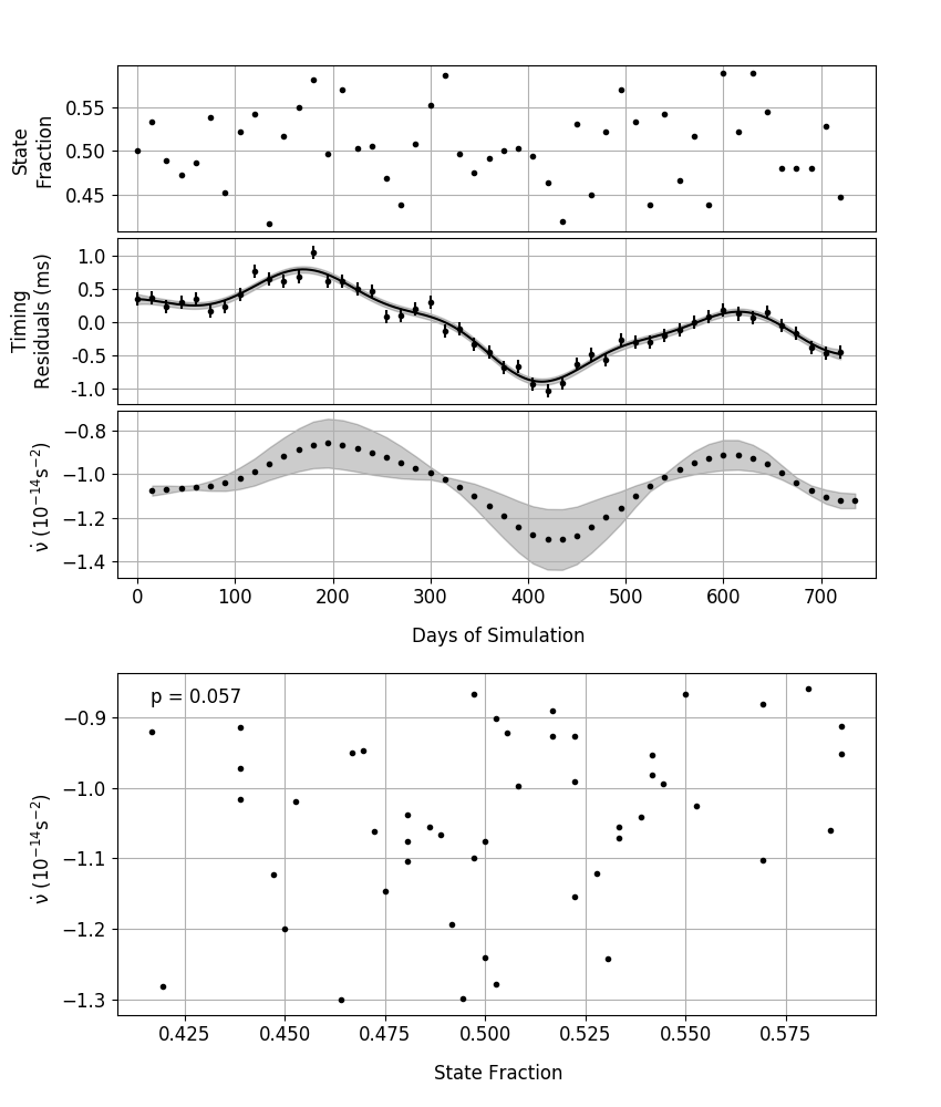
Figure 1: One particular realisation of the simulation in which the state fraction varies stochastically (see Section 4.1), with $\sigma_{\rm SF}=0.03$ and $|\Delta\dot{\nu}|=1\times 10^{-14}$ s^-2. Measurements are made for two simulated years in 15-day increments. Top panel: How the state fraction of the simulated pulsar changes with time. Second panel down: The black dots are the timing residuals with respect to a timing model fit by TEMPO2 (Hobbs et al., 2006) using the simulated TOAs. The TOA measurement uncertainties are 100 $\mu$s. The black line is a GP regression model fit to the timing residuals and the grey shading indicates the $1\sigma$ uncertainty. Third panel down: GP regression allows us to analytically model the second derivative directly from the timing residuals, giving $\dot{\nu}$ with associated fully Bayesian error estimation (see Brook et al. 2016 for details). The $\dot{\nu}$ values are calculated only at points in time where a TOA is produced. Bottom panel: The correlation between the state fraction and $\dot{\nu}$ calculated throughout the simulation. The degree of correlation corresponds to a $p$-value of 0.057 in this realisation, meaning that there is a 5.7% probability that intrinsically non-correlated data would show at least this level of correlation.

We can say a priori, that we would expect no significant correlation between $\dot{\nu}$ and state fraction if any change in $\dot{\nu}$ is so small as to be immeasurable. This would arise in a pulsar with: (i) states with rates of spindown that are too similar, (ii) a state fraction that does not vary over a wide enough range or (iii) a low $S/N$ pulse profile, leading to a large $\sigma_{\rm{TOA}}$. With regards to (i), we already have some information regarding the $\dot{\nu}$ difference ($|\Delta\dot{\nu}|$) in two-state pulsars. In the six Lyne et al. (2010) pulsars, the change in spindown between the two states is approximately between 1 and 10%. In the intermittent pulsars, a $|\Delta\dot{\nu}|$ value as high as 150% has been recorded (Camilo et al., 2012). With regards to (ii), the long term behaviour of the state fraction of mode-changing and nulling pulsars in this context is currently unknown; published mode-changing and nulling fractions, (i.e. the fraction of the observation duration in which a pulsar is in an alternative emission mode) have typically been obtained through single, long-duration observations (e.g. two hours for Wang et al. 2007). In order to learn more about the behaviour of the state fraction and, therefore, realistically constrain and model it within the simulation, we have conducted observations of two nulling pulsars.

3 Constraining State Fraction Variation

Wang et al. (2007) present two-hour observations of 23 pulsars which show evidence of nulling and/or mode-changing behaviour. All observations were made in March or June of 2004, and for each nulling pulsar, a nulling fraction was calculated. In order to learn how a pulsar’s nulling fraction behaves on long timescales, we observed two pulsars in 2014 that were featured in the work by Wang et al. We calculated their nulling fractions and compared them to the 2004 observations to see if and how these values had changed over the intervening decade. The pulsars observed were PSRs J1701$-$3726 and J1727$-$2739. As can be seen in Wang et al., both of these pulsars switch frequently between states of emission and nulling over their two-hour observations. PSR J1701$-$3726 also shows some mode-changing behaviour. Any information regarding the behaviour of nulling fraction on long timescales can help us constrain parameters in the state-changing simulation.

3.1 Observations and Analysis

Both the 2004 and the 2014 data were recorded with one of the Parkes Digital Filterbank systems (PDFB1/2/3/4) with a total bandwidth of 256 MHz in 1024 frequency channels. Radio frequency interference was removed using median-filtering in the frequency domain then manually excising bad sub-integrations. Flux densities have been calibrated by comparison to the continuum radio source 3C 218. The data were then polarisation calibrated for both differential gain and phase, and for cross coupling of the receiver. The MEM method based on long observations of PSR J0437-4715 was used to correct for cross coupling (van Straten, 2004). Flux calibrations from Hydra A were used to further correct the bandpass. After this calibration, profiles were formed of total intensity (Stokes I), and averaged over frequency. PSRs J1701$-$3726 and J1727$-$2739 were observed by Wang et al. for two hours each on 20 March 2004. We observed PSRs J1701$-$3726 for two hours on 2014 March 31 and two hours on 2014 April 02. We observed PSR J1727$-$2739 for two hours on 2014 April 01 and two hours on 2014 April 03. In each observation around 2900 and 5500 single pulses were recorded from PSRs J1701$-$3726 and J1727$-$2739 respectively. GP regression was used to model and subsequently flatten the baseline for each single pulse.

3.2 Nulling Fraction Calculation Method

In order to calculate nulling fraction, Wang et al. (2007) compare flux density histograms for windows centered (i) at pulse phases where the pulsar radio emission occurs and (ii) at phases far from the emission, where only noise is present. When comparing histograms, Wang et al. only consider bins that contain negative flux density values. One group of histogram bins are scaled until comparable with the other; the scaling factor provides the nulling fraction. Often, the best fit after scaling is still poor (depending on S/N and number of null pulses in the histogram). We have opted for a different technique which makes use of all of the flux density information centered at the phase of emission (further details in the following). In any case, more than the absolute nulling fraction, we are interested in seeing how much the fraction changes over time. This should be reflected similarly by both techniques.
For each of the two observed pulsars, we measure the nulling fraction in the following way. By looking at the integrated pulse profile, we can define a phase window which contains all radio emission from the pulsar (see the top panels of Figures 2 and 3). For each single pulse in an observation, we sum the flux density in this phase window. A histogram of the summed flux density values is then constructed for each pulsar observation (see the bottom panels of Figures 2 and 3). Each histogram analysed in this work appears to be either bimodal or trimodal, showing one population of nulls and one or two others of emission in the phase window. There is some overlap between these populations; in order to disentangle them, we fit the sum of multiple components to each histogram using non-linear least squares. The null pulses are modelled by a Gaussian component, and the emitting pulses by one or two log-normal components (Burke-Spolaor et al., 2012). We can calculate the nulling fraction

$$NF=\frac{A_{n}}{A_{n}+A_{e}},$$ (4)

where $A_{n}$ and $A_{e}$ are the areas under the nulling and emission distributions respectively. The area of each component is given by $\sqrt{2\pi}\sigma_{d}H$, where $\sigma_{d}$ is the standard deviation of each distribution and $H$ is its height. The function fitting uncertainty in the nulling fraction is found by propagating the uncertainties of the Gaussian and log-normal component parameters ($\sigma_{d}$ and $H$), as found by the non-linear least squares fits to the histogram.

3.3 PSR J1701$-$3726

PSR J1701$-$3726 is both a nulling and mode-changing pulsar. During a two-hour observation, Wang et al. (2007) observed the pulsar to spend the majority of its time in a mode where a trailing edge profile is much smaller than the rest of the pulse, and a rarer mode in which the pulse profile displays two peaks of roughly equal height. These two emission modes are punctuated by frequent and short nulling periods; the emission variability occurs on minute timescales. The emission windows and the flux density integrated over the whole observation is depicted in the top row of Figure 2 for three observations (one from 2004 and two from 2014). Each panel in the bottom row of the figure shows a histogram for values of the flux density summed over the emission window for each single pulse. It is possible that the nulling state of PSR J1701$-$3726, and each of the two emission states may all have distinct spindown rates and so would not be a good candidate for a continuous monitoring campaign described in this work. However, the observations separated by a decade may still provide useful information regarding the behaviour of nulling fraction on long timescales. Using the distributions fitted to each histogram population and Equation 4, we present the calculated nulling fractions for the three observation of PSR J1701$-$3726 in Table 1.

Figure 2: The pulse profiles and emission histograms for three observations of PSR J1701$-$3726. The dates of the observations are shown at the top. Top panels: The flux density integrated over the whole two-hour observation. The section of the pulse profile shown is the phase window chosen to encompass all emission from the pulsar (see Section 3.2 for details). Bottom panels: Histogram showing the total flux density summed across the emission window (intensity $I$, normalised by mean intensity <$I$>) for each single pulse ($\sim$ 2900 in total). The dashed lines are Gaussian and log-normal functions that are fit to the population of nulls and two populations of pulses respectively. The solid line shows the sum of the dashed lines.

3.4 PSR J1727$-$2739

PSR J1727$-$2739 is a nulling pulsar that shows no signs of mode-changing. Wang et al. (2007) report that the pulsar emits frequent short bursts separated by null intervals, and that this emission variability occurs on minute timescales. The observation-integrated pulse profiles as seen in the top row of Figure 3 show a double peak, with each component being of comparable height. The relative height is not constant in all of observations; for the 2004 observation, the flux density level is highest in the trailing peak, in contrast to the 2014 observations. The bottom row of Figure 3 shows a bimodal histogram for each observation, depicting a population of nulls and one of pulses. The nulling fraction for PSR J1727$-$2739, calculated using Equation 4 is shown in Table 1.

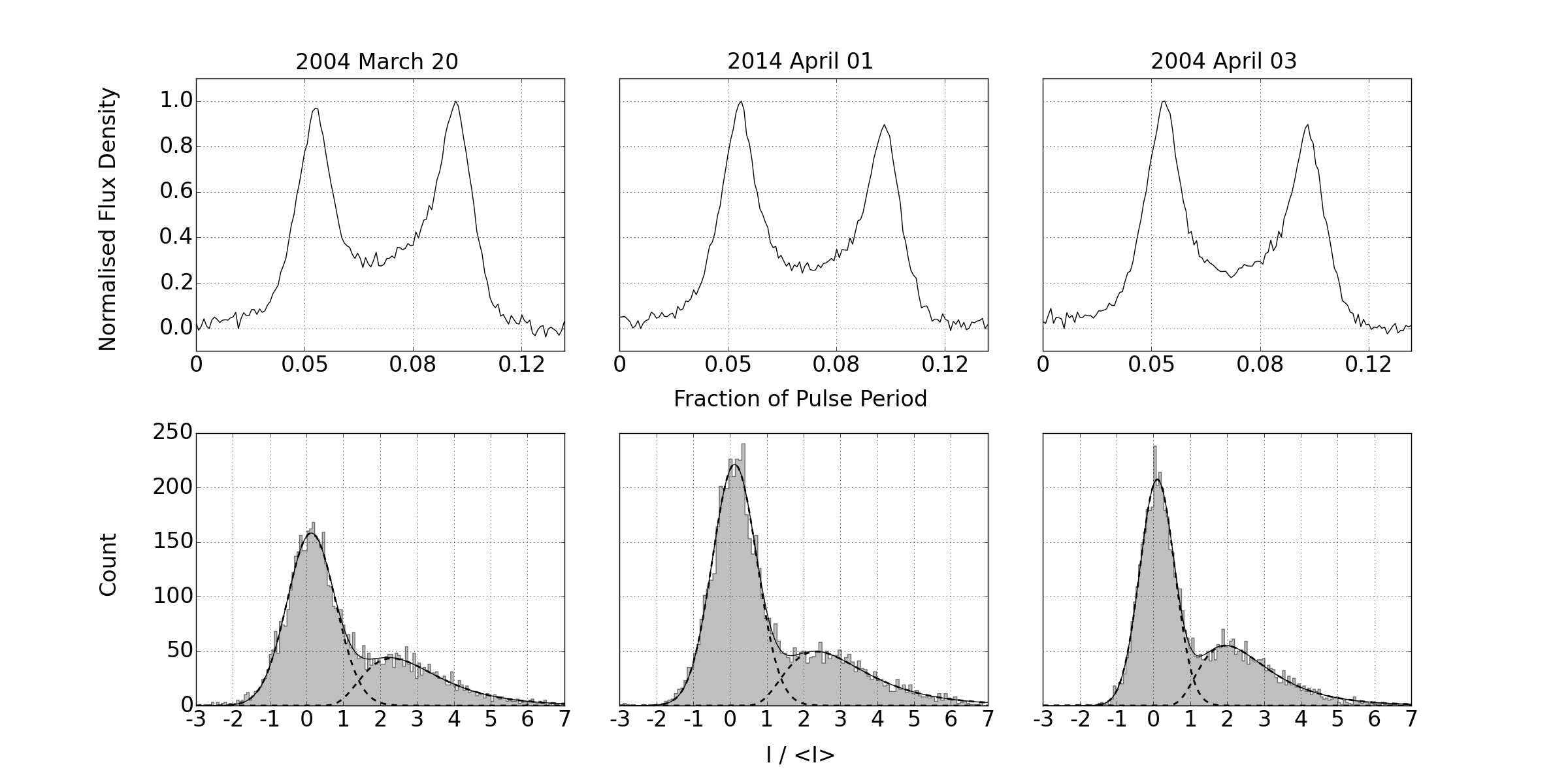
Figure 3: The pulse profiles and emission histograms for three observations of PSR J1727$-$2739. The two-hour observation consisted of $\sim$ 5500 single pulses. The dashed lines are Gaussian and log-normal functions that are fit to a population of nulls and a population of pulses respectively. As Figure 2 otherwise.

3.5 Nulling Fraction Results

Table 1: The calculated nulling fractions for three observations, each of two-hour duration, for PSRs J1701$-$3726 and J1727$-$2739.

PSR J1701$-$3726
Observation Date	Nulling Fraction
2004/03/20	23.4 $\pm$ 5.0%
2014/03/31	24.2 $\pm$ 4.3%
2014/04/02	27.2 $\pm$ 4.6%
PSR J1727$-$2739
Observation Date	Nulling Fraction
2004/03/20	51.7 $\pm$ 7.0%
2014/04/01	57.4 $\pm$ 7.1%
2014/04/03	55.6 $\pm$ 6.8%

The limited data we have do not reveal any significant changes in the nulling fraction of either observed pulsar after measurement uncertainties are taken into consideration. Additionally, even if the underlying nulling fraction does not change, we still expect statistical fluctuations during a two-hour observation. To approximate these, we can model the pulsar emission as a binomial process. Each of our pulsars switches between states of null and emission on roughly minute timescales; a two-hour observation would mean that the number of trials $n$ = 120. We can take the average of our three observations to find the probability $p$ of the pulsar being in a nulling state. For PSR J1701$-$3726, $p$ = 0.23; the standard deviation of the number of nulls in a two-hour observation $\sigma_{n}=\sqrt{np\left(1-p\right)}=4.6$. The standard deviation of the nulling fraction for a two-hour PSR J1701$-$3726 observation, therefore, is $\sim$ 4.6/120 = 3.8%. For PSR J1727$-$2739, $p$ = 0.60 and $\sigma_{n}=5.4$. The standard deviation of the nulling fraction for a two-hour PSR J1727$-$2739 observation is 4.5%. In Table 1 these statistical uncertainties are added in quadrature to the distribution fitting uncertainties. For a 15-day observation (around the length required for a precise measurement of $\dot{\nu}$), the statistical uncertainty of the nulling fraction drops to just $\sim$ 0.3% for both pulsars. We cannot be sure that the changes in nulling fraction that we observe are entirely statistical or due to fitting uncertainties, and not caused by a change (at least in part) in a physical process intrinsic to the pulsar. We consider all of this information when running the state-changing simulation described in the next section.

4 Simulation Results

We simulate a state-changing pulsar with a variety of parameters in order to explore the parameter space over which it would be feasible to detect distinct values of $\dot{\nu}$ in each state. The parameters and their simulated values are summarised in Table 2. We focus on two different scenarios: one in which the state fraction varies stochastically around a certain value, and one in which the state fraction drops systematically with time. In both cases the simulated pulsar begins with a $\nu$ value of 1 Hz, which is constantly decreasing due to a $\dot{\nu}$ value. The standard deviation of the uncertainty of the simulated TOAs is set at 100 $\mu$s. Details of the simulation parameters are presented in Section 2.1.

Table 2: Variable parameters in the pulsar state-changing simulation.

Description	Parameter	Value
Initial rotation frequency of the pulsar	$\nu_{0}$	1 Hz
Difference in the spindown rate of the two states	$|\Delta\dot{\nu}|$	10-18 to 10-14 s-2
Stochastic state fraction standard deviation	$\sigma_{\rm SF}$	0.01 to 0.1
Systematic rate of state fraction drop	-	0.005 to 0.05 per year
Uncertainty of TOA measurements	$\sigma_{\rm TOA}$	$1\times 10^{-4}$ seconds
Time between possible state changes	-	1 hour
Time between $\nu$ and SF measurements	-	15 days
Simulation length	-	1 and 2 years

4.1 Stochastic Changes in State Fraction

In one version of the simulation, we make the assumption that the underlying state fraction of the pulsar has a mean value (which we set to 0.5) and a standard deviation which we vary between 0.01 to 0.1 (holding the value fixed for the length of the simulated experiment). We will see that if we draw the state fraction from a distribution with a standard deviation too much above or below these values, then identifying the different $\dot{\nu}$ values of a state changing pulsar becomes either impossible or trivial respectively (over most of our chosen range of $|\Delta\dot{\nu}|$ values). The value of the underlying state fraction stays fixed for 15 days; the period over which $\dot{\nu}$ and the observed state fractions are evaluated. The simulated pulsar has the opportunity to change between a nulling or emitting state every hour of the simulation. This is determined by the generation of a random number, weighted by the value of the underlying state fraction at that point in the simulation. The frequency with which the state of the pulsar is permitted to change has an effect in terms of the standard deviation of the observed state fraction in any 15-day evaluation period: $\sigma_{SF}\propto\sqrt{T}$, where $T$ is the nulling/emitting timescale. This is discussed further in Section 5. The opportunity to change every simulated hour was chosen to find a balance between simulating a realistic state-changing pulsar and short computation time.
As inferred in Section 2.1, another important indicator of whether different spindown states can be detected is how different the $\dot{\nu}$ values of the two states are. For this simulation, $|\Delta\dot{\nu}|$ has values between 10^-18 and 10^-14 s^-2. These values are reasonable when considering the $|\Delta\dot{\nu}|$ values observed in known state switching and intermittent pulsars (Kramer et al., 2006; Lyne et al., 2010; Camilo et al., 2012; Lorimer et al., 2012; Brook et al., 2014; Brook et al., 2016; Lyne et al., 2017).
The pulsar is simulated to be observed for one year and also for two years. As the observed state fraction and average $\dot{\nu}$ value are measured every 15 days, the simulation generates 24 and 48 pairs of data points for the one- and two-year simulations respectively. The Pearson correlation coefficient of the pairs is then calculated along with a $p$-value, which indicates the probability that no correlation is detected. Figures 4 (one year) and 5 (two years) show the mean $p$-values ($\bar{p}$) for a range of state fractions and $|\Delta\dot{\nu}|$. For each location in parameter space in these figures, 100 $p$-values were calculated and the resulting $\bar{p}$-value and standard deviation are shown.

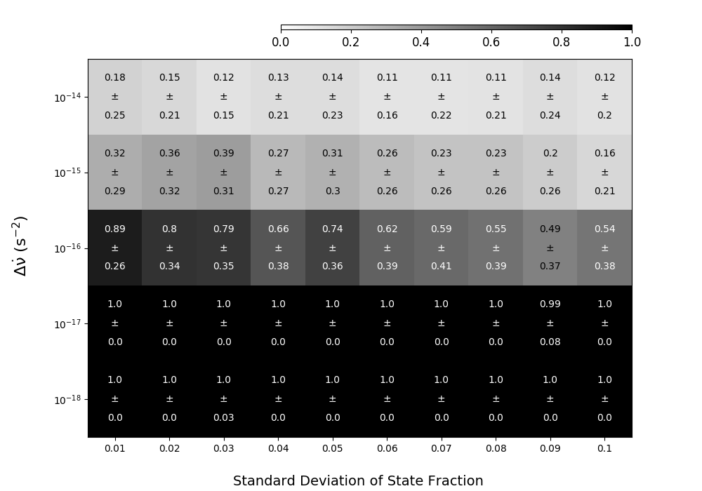
Figure 4: The correlation of $\dot{\nu}$ and state fraction over a range of parameters for simulations of one-year continuous observations. For each permutation of parameters the mean and standard deviation of 100 $p$-values is shown. A smaller $\bar{p}$-value reflects a lower probability that non-correlated data would show at least an equal level of correlation and produces a lighter grey-scale square. The realisations in which the GP modelled $\dot{\nu}$ as having no change over the duration of the simulation necessarily produce a Pearson correlation coefficient of 0 and, therefore, $p$-value = 1.0. If all 100 contributing models have flat $\dot{\nu}$ values, then $\bar{p}$-value = 1.0 and the standard deviation will be 0.0, as seen in some regions of parameter space with small $|\Delta\dot{\nu}|$ values.

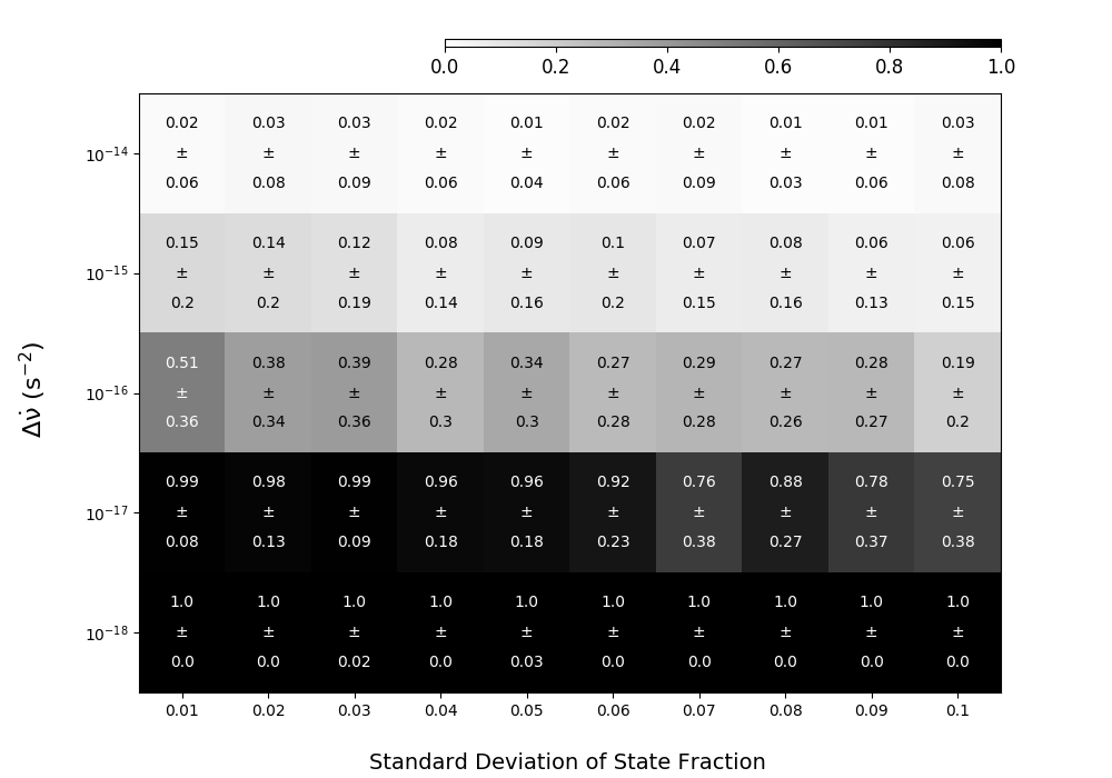
Figure 5: As Figure 4, but for simulations of two-year continuous observations.

4.2 Systematic Changes in State Fraction

In a second version of the simulation, we make the assumption that the underlying state fraction systematically drops over time; we explore the parameter space over which the drop rate is between 0.005 and 0.05 per year. This range is informed by our observations of PSRs J1701$-$3726 and J1727$-$2739; 0.005 per year amounts to a drop in state fraction of $\sim$ 5% over the span between our 2004 and 2014 nulling fraction calculations. It is possible for a change of this magnitude to be hidden in PSRs J1701$-$3726 and J1727$-$2739 by measurement uncertainties and statistical fluctuations. Values above our upper value of 0.05 per year are considered unrealistically large. All other parameters are also unchanged from the stochastic simulation including $|\Delta\dot{\nu}|$ which is again simulated between 10^-18 and 10^-14 s^-2. The results from the one and two year simulations are shown in Figures 6 and 7 respectively.

Figure 6: As Figure 4, but for simulations of one-year continuous observations during which the state fraction systematically drops.

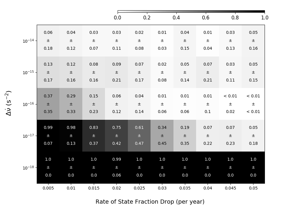
Figure 7: As Figure 4, but for simulations of two-year continuous observations during which the state fraction systematically drops.

5 Discussion

The state-changing simulation shows us that our best opportunity to infer different $\dot{\nu}$ states in nulling or mode-changing pulsars, is by observing those with high $|\Delta\dot{\nu}|$ values and with a state fraction that is highly variable or displays significant systematic changes. If the intrinsic state fraction of a pulsar has a steady mean around which it varies stochastically with time, then a large variance of the state fraction improves our sensitivity to the detection of distinct $\dot{\nu}$ states. The situation is not so simple when we consider a pulsar with a systematically varying state fraction. There is now a trade-off between a state fraction with a large variance and one with smaller variance which more faithfully follows the systematic trend. The optimum variance of state fraction in each systematic case is dependent on the nature of the trend. This is illustrated in Figure 8 which compares the evolution of stochastically and systematically varying state fractions. Both simulated data sets show a similar level of correlation between the state fraction and $\dot{\nu}$, with each having a final $p$-value of 0.11.

A pulsar having similar properties to those in our simulation and a $|\Delta\dot{\nu}|$ value of at least $10^{-14}$ s^-2 will allow us to detect correlation between state fraction and $\dot{\nu}$ with 95% confidence within a two-year observing campaign. This is equivalent to a pulsar with $\dot{\nu}=-10^{-13}$ s^-2 which changes by 10% between emission states. Although above average, there are still many known radio pulsars with $|\dot{\nu}|$ $\geq$ $10^{-13}$ s^-2. Of course, in pulsars with even higher values of $\dot{\nu}$, a lower percentage change is needed to satisfy our $|\Delta\dot{\nu}|$ requirement of at least $10^{-14}$ s^-2 when the state switch occurs. If the variability of the state fraction is very high, or if it changes in a systematic rather than a stochastic way, then any correlation between state fraction and $\dot{\nu}$ may be confidently seen even when $|\Delta\dot{\nu}|$ is lower than $10^{-14}$ s^-2.

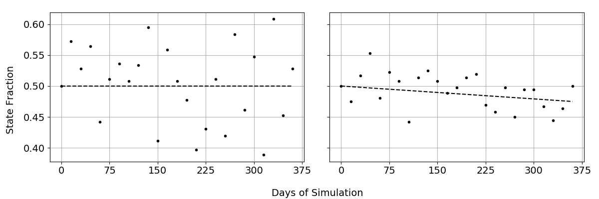
Figure 8: A comparison of stochastically and systematically varying state fractions. The left panel shows stochastic evolution, with $\sigma_{\rm SF}=0.05$. The underlying mean value is shown by the dashed line. The right panel has a systematic trend; the underlying rate of state fraction drop is 0.025 per year, as shown by the dashed line. The state fractions in the left panel correlates with their resulting $\dot{\nu}$ values to a level of $p=0.1132$. For the right panel $p=0.1139$.

Shaw et al. (2018) show that the transitions only become reliably detectable when they occur on timescales greater than approximately a month. They also show that using changes in a pulsar’s emission to provide information about the transition epoch (assuming rotation-emission correlation in the pulsar) is advantageous for finding transition parameters when the $\dot{\nu}$ jumps are low amplitude and closely spaced in time. Although we rely on statistical rather than direct measurement techniques, in some sense our work is an extrapolation of these concepts; we are able to detect rotational changes that occur right down to the shortest timescales (the pulse period) and our ability to do so is completely reliant on information provided by the continuous monitoring of the emission state of the pulsar.

5.1 Caveats

• When setting 100 $\mu$s as a typical level of TOA measurement uncertainty, we only considered template-fitting errors due to radiometer noise. However, phenomena such as pulse jitter (Cordes & Downs, 1985) are known to be present in some pulsars. This is the stochastic, broadband, single-pulse variations that are intrinsic to the pulsar emission process and affect the shape of the integrated pulse profile. The presence of jitter would increase the TOA measurement uncertainty and hinder the detection of a correlation between $\dot{\nu}$ and state fraction. However, TOA uncertainty due to jitter

  $$\sigma_{J}\propto\frac{1}{\sqrt{n}},$$ (5)

  where n is the number of pulses that make up the pulse profile used to calculate the TOA. As we are proposing to calculate TOAs over a 15 day span, the many integrated pulses ensure that this uncertainty is small. From Equation 5 of Cordes & Shannon (2010) we calculate that the TOA measurement error due to jitter for a typical pulsar with $\nu$ = 1 Hz, calculated over 15 days is $\sim$ 2 $\mu$s. When this jitter uncertainty is added in quadrature to the template-fitting uncertainties, the latter will dominate. Timing uncertainty induced by jitter can, therefore, largely be ignored in our proposed experiment.

• The state-changing simulation does not include the injection of the timing irregularity known as timing noise. This is a term given to the unexplained, quasi-periodic wander from the modelled rotational behaviour of a pulsar. There have been numerous processes proposed to explain timing noise, such as the presence of an asteroid belt (Shannon et al., 2013), or planetary systems (Thorsett et al., 1999). Both Kramer et al. (2006) and Lyne et al. (2010) showed that timing noise can be produced by unmodelled magnetospheric state changes that simultaneous affect a pulsar’s emission and rotation (in intermittent pulsars and state-switching pulsars respectively). If the short-term emission variability in nulling and mode-changing pulsars is also accompanied by spindown rate changes, then timing noise will also be intrinsic to these pulsars and hence may naturally emerge from our simulations.

• The $|\Delta\dot{\nu}|$ values in the simulations were based on state-switching pulsars (Lyne et al., 2010) which have reported fractional changes in $\dot{\nu}$ of between approximately 1-10%, and intermittent pulsars (Kramer et al., 2006; Camilo et al., 2012; Lorimer et al., 2012; Lyne et al., 2017) which have fractional changes up to around 150%. At present, we do not know if the fractional $\dot{\nu}$ changes in nulling and mode-changing pulsar will be comparable, if indeed they change at all. Although they have similar timescales, the radio emission in intermittent pulsars appears to cease completely (unlike state-switching pulsars). By analogy, we might expect that nulling pulsars may also have larger fractional $\dot{\nu}$ changes than mode-changing pulsars when their shorter timescale state changes occur.

• When modelling how the pulsar state fraction changes with time, the variable input parameter for the simulation is (i) how the underlying state fraction changes with time. When we subsequently measure the output state fraction, however, the result will be a combination of (i) and (ii) the standard deviation of the measurements due to the statistics of finite observation length. If the underlying state fraction has an unchanging value, the measurements will vary around this mean; the standard deviation of the state fraction in this case would depend on how many state changes take place during an observation, and can be approximated as a binomial process. As an example, if the underlying state fraction of a pulsar is unchanging at 0.5, then a 15-day observation in which there is an hourly opportunity to switch states (as in our simulation) would constitute 360 trials. Therefore, $\sigma_{\rm STATE}=\sqrt{360\cdot 0.5\cdot 0.5}/360=2.6\%$. If the pulsar was able to switch states each minute, then $\sigma_{\rm STATE}$ drops to 0.3%. As we want to maximise the variance of state fraction in order for us to detect any correlation between state fraction and $\dot{\nu}$, it would be preferential for us to observe a pulsar in which the state changes occur on as long a timescale as possible. Conversely, when considering a pulsar in which the state changes occur on timescales less than an hour, our results matrices (Figures 4 to 7) will be optimistic, especially in regions where the standard deviation of the underlying state fraction (Figures 4 and 5) or rate of state fraction drop (Figures 6 and 7) is low.

Even in the most pessimistic case, in which a continuous monitoring campaign of a state-changing pulsar does not yield any correlation between $\dot{\nu}$ and state fraction, this would allow an upper limit to be placed on $|\Delta\dot{\nu}|$. In addition to this, such a campaign will produce a unique data set and provide information regarding how the state fraction of nulling or mode-changing pulsars evolves over timescales from days to years. To carry out this experiment in practice, the observing instrument need only monitor continuously for as long as it takes to make a precise measurement of $\dot{\nu}$ (around 15 days) and the corresponding state fraction for the observation span. Each such pair of data points can be recorded in this way, with no requirement for the observing spans to be contiguous. Therefore, the observing instrument does not need to be employed continuously for many months. In principle, a bright circumpolar pulsar could be observed with a relatively high $S/N$ using a sub-array of a radio interferometer rather than a dedicated single dish telescope. Any instrument must be sufficiently sensitive to obtain the necessary $S/N$ to obtain precise TOAs and also to be able to distinguish between different emission modes.

6 Conclusions

We have simulated the parameters over which a continuous monitoring campaign of a state-changing radio pulsar could reveal distinct spindown rates in each emission state. All other things being equal, the simulation results have shown us that the crucial parameters for success are (i) a long monitoring campaign, (ii) a state fraction that is either highly variable or follows a significant systematic trend and (iii) a large difference between state spindown rates. The latter will not be known before the experiment takes place, and (ii) may only be poorly constrained at best; if a pulsar is known to have a predictable systematic state fraction, then it may be possible to forego continuous monitoring altogether and just take enough observations to compare $\dot{\nu}$ against the predicted state fraction changes. Assuming no knowledge of (ii), in order to maximise our chances of success in revealing distinct rotational states, we would ideally monitor a bright, circumpolar nulling pulsar with a high rate of spindown, a long timescale for nulls and a nulling fraction close to 50% to maximise the statistical variance of the nulling fraction.

References

- Ambikasaran et al. (2015) Ambikasaran S., Foreman-Mackey D., Greengard L., Hogg D. W., O’Neil M., 2015, IEEE Transactions on Pattern Analysis and Machine Intelligence, 38
- Backer (1970a) Backer D. C., 1970a, Nature, 228, 42
- Backer (1970b) Backer D. C., 1970b, Nature, 228, 1297
- Biggs (1992) Biggs J. D., 1992, ApJ, 394, 574
- Brook et al. (2014) Brook P. R., Karastergiou A., Buchner S., Roberts S. J., Keith M. J., Johnston S., Shannon R. M., 2014, ApJ, 780, L31
- Brook et al. (2016) Brook P. R., Karastergiou A., Johnston S., Kerr M., Shannon R. M., Roberts S. J., 2016, MNRAS, 456, 1374
- Burke-Spolaor et al. (2012) Burke-Spolaor S., et al., 2012, MNRAS, 423, 1351
- Camilo et al. (2012) Camilo F., Ransom S. M., Chatterjee S., Johnston S., Demorest P., 2012, ApJ, 746, 63
- Cordes & Downs (1985) Cordes J. M., Downs G. S., 1985, ApJS, 59, 343
- Cordes & Shannon (2010) Cordes J. M., Shannon R. M., 2010, arXiv e-prints 1010.3785),
- Hobbs et al. (2006) Hobbs G. B., Edwards R. T., Manchester R. N., 2006, MNRAS, 369, 655
- Hobbs et al. (2016) Hobbs G., et al., 2016, MNRAS, 456, 3948
- Kramer et al. (2006) Kramer M., Lyne A. G., O’Brien J. T., Jordan C. A., Lorimer D. R., 2006, Science, 312, 549
- Lorimer et al. (2012) Lorimer D. R., Lyne A. G., McLaughlin M. A., Kramer M., Pavlov G. G., Chang C., 2012, ApJ, 758, 141
- Lyne et al. (2010) Lyne A., Hobbs G., Kramer M., Stairs I., Stappers B., 2010, Science, 329, 408
- Lyne et al. (2017) Lyne A. G., et al., 2017, ApJ, 834, 72
- McLaughlin et al. (2006) McLaughlin M. A., et al., 2006, Nature, 439, 817
- Ritchings (1976) Ritchings R. T., 1976, MNRAS, 176, 249
- Shannon et al. (2013) Shannon R. M., et al., 2013, ApJ, 766, 5
- Shaw et al. (2018) Shaw B., Stappers B. W., Weltevrede P., 2018, MNRAS, 475, 5443
- Thorsett et al. (1999) Thorsett S. E., Arzoumanian Z., Camilo F., Lyne A. G., 1999, ApJ, 523, 763
- Wang et al. (2007) Wang N., Manchester R. N., Johnston S., 2007, MNRAS, 377, 1383
- van Straten (2004) van Straten W., 2004, ApJS, 152, 129