Master integrals for the NNLO virtual corrections to $q\bar{q}\rightarrow t\bar{t}$ scattering in QCD: the non-planar graphs

Abstract

We complete the analytic evaluation of the master integrals for the two-loop non-planar box diagrams contributing to the top-pair production in the quark-initiated channel, at next-to-next-to-leading order in QCD. The integrals are determined from their differential equations, which are cast into a canonical form using the Magnus exponential. The analytic expressions of the Laurent series coefficients of the integrals are expressed as combinations of generalized polylogarithms, which we validate with several numerical checks. We discuss the analytic continuation of the planar and the non-planar master integrals, which contribute to $q{\bar{q}}\to t{\bar{t}}$ in QCD, as well as to the companion QED scattering processes $ee\to\mu\mu$ and $e\mu\to e\mu$.

1 Introduction

The top quark is the heaviest elementary matter particle. Its large production rate at the CERN LHC enables precision studies, thereby testing the Standard Model of particle physics at an unprecedented level, and potentially uncovering indirect evidence for new physics effects. Precision measurements of top quark observables Aad:2015mbv ; Aaboud:2017fha ; Khachatryan:2015oqa ; Sirunyan:2018wem must be confronted with equally precise theory predictions, thereby requiring the perturbation theory descriptions of these observables to be extended to high orders.

The available second-order (next-to-next-to-leading order, NNLO) QCD corrections to the top quark pair production process (initially for the total cross section Czakon:2013goa and subsequently for differential distributions Czakon:2014xsa ; Czakon:2015owf ; Czakon:2016dgf ; Catani:2019iny ) deliver a competitive level of theory predictions, and are enabling a multitude of precision studies with top quark pairs. A key ingredient to these calculations are the two-loop QCD corrections to the matrix elements for top pair production in quark-antiquark annihilation and gluon fusion. While numerical representations of these two-loop matrix elements were derived already some time ago Baernreuther:2013caa ; Chen:2017jvi , only partial analytical results are available for them up to now Bonciani:2008az ; Bonciani:2009nb ; Bonciani:2010mn ; Bonciani:2013ywa (and used in partial validations Abelof:2014fza ; Abelof:2015lna of the total NNLO cross section calculation). Such analytical results allow in-depth investigations into the structure of the matrix elements, enabling to investigate limiting behaviors and analyticity structures, as well as providing an independent approach to their numerical evaluation. Up to now, full results for the two-loop top quark production matrix elements could not be derived due to incomplete knowledge on the relevant two-loop Feynman integrals. Important steps towards the evaluation of the missing two-loop functions have been recently undertaken in vonManteuffel:2017hms ; Adams:2018bsn ; Adams:2018kez ; Chen:2019zoy .

In this work, we complete the task of determining all the non-planar two-loop functions that are needed for the evaluation of the scattering amplitudes for the quark initiated channel $q{\bar{q}}\to t{\bar{t}}$ at NNLO in QCD. Owing to the large value of the top mass compared to the mass of the two incoming quarks, which we suppose to have different flavor, we treat the latter as massless.

The results of this paper represent an additional milestone of the research program dedicated to the two-loop QCD and QED corrections to the interaction of two fermionic currents, that was initiated with the study of the muon-electron scattering, in the context of the MUonE experiment Calame:2015fva ; Abbiendi:2016xup , which is currently under evaluation at CERN.

By following the same the path of the calculation of two-loop integrals for $\mu e\to\mu e$ and the crossing-related processes considered in Mastrolia:2017pfy ; DiVita:2018nnh , we adopt a consolidated strategy Henn:2013pwa ; Argeri:2014qva , which was proven to be particularly effective in the context of multi-loop integrals that involve multiple kinematic scales Argeri:2014qva ; DiVita:2014pza ; Bonciani:2016ypc ; DiVita:2017xlr ; Mastrolia:2017pfy ; DiVita:2018nnh ; Primo:2018zby . By means of integration-by-parts identities (IBPs) Tkachov:1981wb ; Chetyrkin:1981qh ; Laporta:2001dd , we identify a set of 52 master integrals (MIs) that we evaluate analytically, through the differential equations method Barucchi:1973zm ; Kotikov:1990kg ; Remiddi:1997ny ; Gehrmann:1999as . In particular, we consider an initial set of MIs that obey a system of first-order differential equations (DEQs) in two independent kinematic variables that is linear in the space-time dimensions $d$. The system is subsequently cast in canonical form Henn:2013pwa by means of the Magnus exponential matrix Argeri:2014qva . The matrix associated to the canonical system, where the dependence on $(d-4)$ is factorized from the kinematics, is a logarithmic differential form, which – once parametrized in terms of suitable variables – has a polynomial alphabet, constituted of eleven letters. Therefore, the canonical MIs are found to admit a Taylor series representation around $d=4$, whose coefficients are combinations of generalized polylogarithms (GPLs) Goncharov:polylog ; Remiddi:1999ew ; Gehrmann:2001pz ; Vollinga:2004sn . The otherwise unknown integration constants are determined either from the knowledge of the analytic expression of the MIs in special kinematic configurations or by imposing their regularity at the pseudo-thresholds of the DEQs. Finally, we show how the MIs, that we initially compute in an unphysical region, can be analytically continued to the top-pair production region. Due to the non-trivial structure of their branch-cuts, the analytic continuation of the two-loop functions considered in this paper represents a paradigmatic case, that can be useful for the study of other planar and non-planar diagrams that involve massive particles. As a byproduct of the current analysis, we obtain the analytic continuation to the physical region of the functions required for the $\mu e\to\mu e$ and $ee\to\mu\mu$ scattering in QED Mastrolia:2017pfy ; DiVita:2018nnh .

In the completion of this calculation, we benefited from publicly available software dedicated to multi-loop calculus. The IBPs decomposition and the generation of the dimension-shifting identities and DEQs obeyed by the MIs have been performed with the packages Kira Maierhoefer2018a , LiteRed Lee:2012cn ; Lee:2013mka and Reduze vonManteuffel:2012np ; vonManteuffel:2014qoa . The analytic expressions of the MIs, which we evaluate numerically with the help of GiNaC Bauer:2000cp , were successfully tested against the numerical values provided either by SecDec Borowka:2015mxa or, for the most complicated 7-denominator topologies, by an in-house algorithm.

Beside these important validations, our results have been successfully compared against the computation of the master integrals relevant to the same integral topologies expressed in a different basis set, independently obtained by Becchetti, Bonciani, Casconi, Ferroglia, Lavacca and von Manteuffel Becchetti:2019tjy , published in tandem to the current manuscript.

The remainder of the paper is organized as follows: in section 2 we set our notation and conventions for the non-planar two loop functions. In section 3, we present the system of DEQs obeyed by the MIs and their solutions in the unphysical region. In section 4, we study the analytic continuation of the MIs to the physical region. Finally, in section 5, we discuss the numerical evaluation of the 7-denominator integrals. Appendix A contains the coefficients of the linear combinations of MIs that satisfy a canonical system of DEQs.

The analytic expressions of the considered MIs are given in the ancillary files accompanying the arXiv version of this publication.

2 The non-planar four-point topology

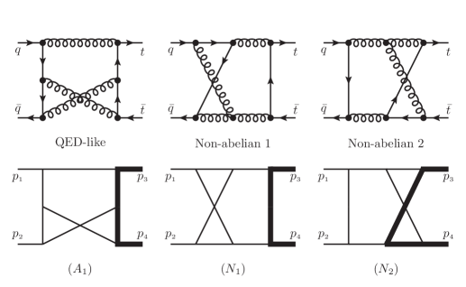
Figure 1: Representative non-planar diagrams contributing at two-loops to $q(p_{1})+\bar{q}(p_{2})\to t(p_{3})+\bar{t}(p_{4})$ (top row), and the associated integral families (bottom row). Massive propagators and external legs are depicted using thick lines. The diagrams have been drawn with axodraw2 Collins2016 .

In this paper, we complete the determination of the Feynman integrals for the $q\bar{q}\rightarrow t\bar{t}$ scattering process

$$q(p_{1})+\bar{q}(p_{2})\to t(p_{3})+\bar{t}(p_{4})\,,$$ (1)

with kinematics specified by

$$p_{1}^{2} =p_{2}^{2}=0\,,\quad p_{3}^{2}=p_{4}^{2}=m^{2}\,,$$

$$s=(p_{1}+p_{2})^{2}\,,\quad t =(p_{2}-p_{3})^{2}\,,\quad u=(p_{1}-p_{3})^{2}=2m^{2}-t-s\,,$$ (2)

where $m$ is the top quark mass. The full set of two-loop three-point integrals that are involved in the process has been known for some time Gehrmann:2001ck ; Bonciani:2003te ; Bonciani:2003hc ; Bonciani:2008wf ; Asatrian:2008uk ; Beneke:2008ei ; Bell:2008ws ; Huber:2009se , as well all the relevant planar four-point functions Bonciani:2008az ; Bonciani:2009nb ; Mastrolia:2017pfy . On top of these contributions, the evaluation of the full double-virtual matrix element requires the computation of two-loop non-planar Feynman diagrams. Representative non-planar diagrams are shown in the top row of figure 1. In the bottom row, we also show the integral families onto which we map those diagrams. Massive propagators and external legs are depicted using thick lines. The MIs for the QED-like family $A_{1}$ are already available in the literature, as they have been studied in the context of the NNLO QED corrections to $ee\mu\mu$ processes (with suitable redefinitions of the momenta and of the Mandelstam invariants). In particular, they have been first computed in DiVita:2018nnh (in an unphysical region, to be analytically continued), and later in Lee:2019lno (directly in the heavy-fermion-production kinematic region). As for the genuine QCD contributions, the MIs for family $N_{1}$ have been computed in Manteuffel2013 , while the MIs for family $N_{2}$ are the subject of the present publication.

In arbitrary $d$ dimensions, we parametrize the integrals of family $N_{2}$ as

$$I^{[d]}(n_{1},\ldots,n_{9})\equiv\int\widetilde{\mathrm{d}^{d}k_{1}}\widetilde{\mathrm{d}^{d}k_{2}}\,\frac{1}{D_{1}^{n_{1}}\ldots D_{9}^{n_{9}}}\,,$$ (3)

where $D_{i}$ are the inverse scalar propagators

$$D_{1}=k_{1}^{2},\quad D_{2}=k_{2}^{2}-m^{2},\quad D_{3}=(k_{2}-p_{3})^{2},\quad D_{4}=(k_{1}-p_{2})^{2},$$

$$D_{5}=(k_{1}-p_{3}-p_{4})^{2},\quad D_{6}=(k_{1}-k_{2})^{2}-m^{2},\quad D_{7}=(k_{1}-k_{2}-p_{4})^{2},$$

$$D_{8}=(k_{1}-p_{3})^{2},\quad D_{9}=(k_{2}-p_{2})^{2}\,,$$ (4)

with $k_{1}$ and $k_{2}$ denoting the loop momenta.

The analytic calculation described in section 3 is performed by expanding the MIs around $d=4$, while the numerical evaluation presented in section 5 as a check of our results is carried over around $d=6$. Therefore, we set $\epsilon\equiv(d_{*}-d)/2$, where $d_{*}=4$ and $d_{*}=6$ according to the case. In addition, we define our integration measure as

$$\widetilde{\mathrm{d}^{d}k}={} \frac{\mathrm{d}^{d}k}{i\pi^{d/2}\,\Gamma\left(1+\epsilon\right)}\left(\frac{m^{2}}{\mu^{2}}\right)^{\epsilon}\,,$$ (5)

where $\mu$ is the ’t Hooft scale of dimensional regularization. In this convention, the two-loop tadpole integral $\epsilon^{2}I^{[4-2\epsilon]}(0,2,0,0,0,2,0,0,0)$ is normalized to $1$.

3 Solution of the system of differential equations

From the IBP reduction of the two-loop integrals belonging to the family defined in eqs. (3)-(4) we identify a basis of 52 MIs. We determine the analytic expressions of the MIs by solving their DEQs in the Mandelstam invariants $s$, $t$ and the top quark mass $m^{2}$. IBPs and DEQs have been derived by requiring the external legs to be on-shell. The solution of the DEQs in terms of known functions is facilitated by the following reparametrization of the kinematics:

$$\frac{u-m^{2}}{t-m^{2}}=-\frac{z^{2}}{w},\qquad\frac{s}{m^{2}}=-\frac{(1-w)^{2}}{w}\,,$$ (6)

where the constraint on the Mandelstam invariants $s+t+u=2m^{2}$ is understood. The dimensionless variables ${w}$ and ${z}$ appearing in eq. (6) were already introduced in DiVita:2018nnh for the computation of the MIs of the non-planar family $A_{1}$ (modulo the relabeling $s\leftrightarrow t$). Also in this case, the above change of variables rationalizes the coefficients of the canonical DEQs, hence allowing to express the MIs in terms of GPLs.

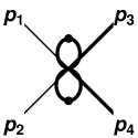
(a) $\mathcal{T}_{1}$

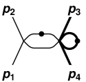
(b) $\mathcal{T}_{2}$

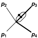
(c) $\mathcal{T}_{3}$

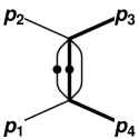
(d) $\mathcal{T}_{4}$

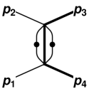
(e) $\mathcal{T}_{5}$

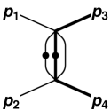
(f) $\mathcal{T}_{6}$

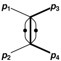
(g) $\mathcal{T}_{7}$

(h) $\mathcal{T}_{8}$

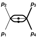
(i) $\mathcal{T}_{9}$

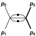
(j) $\mathcal{T}_{10}$

(k) $\mathcal{T}_{11}$

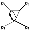
(l) $\mathcal{T}_{12}$

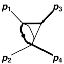
(m) $\mathcal{T}_{13}$

(n) $\mathcal{T}_{14}$

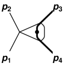
(o) $\mathcal{T}_{15}$

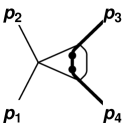
(p) $\mathcal{T}_{16}$

(q) $\mathcal{T}_{17}$

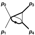
(r) $\mathcal{T}_{18}$

(s) $\mathcal{T}_{19}$

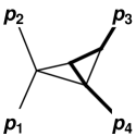
(t) $\mathcal{T}_{20}$

(u) $\mathcal{T}_{21}$

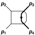
(v) $\mathcal{T}_{22}$

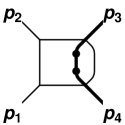
(w) $\mathcal{T}_{23}$

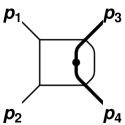
(x) $\mathcal{T}_{24}$

(y) $\mathcal{T}_{25}$

Figure 2: The first 25 MIs $\mathcal{T}_{1,\ldots,25}$ for the two-loop non-planar topology $N_{2}$ of figure 1. Massless propagators are represented by think lines and massive propagators by thick ones. Each dot indicates an additional power of the corresponding propagator. Numerator insertions are indicated explicitly on top of each diagram.

(a) $\mathcal{T}_{26}$

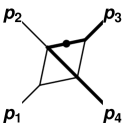
(b) $\mathcal{T}_{27}$

(c) $\mathcal{T}_{28}$

(d) $\mathcal{T}_{29}$

(e) $\mathcal{T}_{30}$

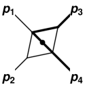
(f) $\mathcal{T}_{31}$

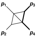
(g) $\mathcal{T}_{32}$

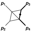
(h) $\mathcal{T}_{33}$

(i) $\mathcal{T}_{34}$

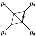
(j) $\mathcal{T}_{35}$

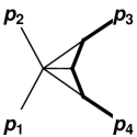
(k) $\mathcal{T}_{36}$

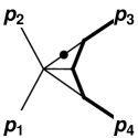
(l) $\mathcal{T}_{37}$

(m) $\mathcal{T}_{38}$

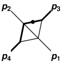
(n) $\mathcal{T}_{39}$

(o) $\mathcal{T}_{40}$

(p) $\mathcal{T}_{41}$

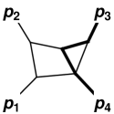
(q) $\mathcal{T}_{42}$

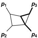
(r) $\mathcal{T}_{43}$

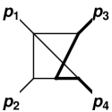
(s) $\mathcal{T}_{44}$

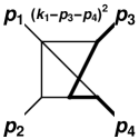
(t) $\mathcal{T}_{45}$

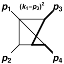
(u) $\mathcal{T}_{46}$

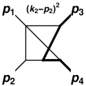
(v) $\mathcal{T}_{47}$

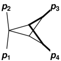
(w) $\mathcal{T}_{48}$

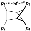
(x) $\mathcal{T}_{49}$

(y) $\mathcal{T}_{50}$

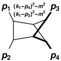
(z) $\mathcal{T}_{51}$

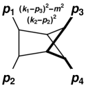
(aa) $\mathcal{T}_{52}$

Figure 3: The remaining 27 MIs $\mathcal{T}_{26,\ldots,52}$ for the two-loop non-planar topology $N_{2}$ of figure 1. The conventions are the same as in figure 2.

3.1 Differential equations for master integrals

We determine a canonical basis of MIs in $d=4-2\epsilon$ through the Magnus exponential algorithm described in Argeri:2014qva ; DiVita:2014pza . As a starting point, we identify a set of 52 independent integrals $\text{F}_{i}$, whose DEQs depend linearly on the dimensional regularization parameter $\epsilon$,

$$\text{F}_{1} =\epsilon^{2}\,\mathcal{T}_{1}\,, \text{F}_{2} =\epsilon^{2}\,\mathcal{T}_{2}\,, \text{F}_{3} =\epsilon^{2}\,\mathcal{T}_{3}\,,$$

$$\text{F}_{4} =\epsilon^{2}\,\mathcal{T}_{4}\,, \text{F}_{5} =\epsilon^{2}\,\mathcal{T}_{5}\,, \text{F}_{6} =\epsilon^{2}\,\mathcal{T}_{6}\,,$$

$$\text{F}_{7} =\epsilon^{2}\,\mathcal{T}_{7}\,, \text{F}_{8} =\epsilon^{2}\,\mathcal{T}_{8}\,, \text{F}_{9} =\epsilon^{2}\,\mathcal{T}_{9}\,,$$

$$\text{F}_{10} =\epsilon^{2}\,\mathcal{T}_{10}\,, \text{F}_{11} =\epsilon^{3}\,\mathcal{T}_{11}\,, \text{F}_{12} =\epsilon^{2}\,\mathcal{T}_{12}\,,$$

$$\text{F}_{13} =\epsilon^{3}\,\mathcal{T}_{13}\,, \text{F}_{14} =\epsilon^{2}\,\mathcal{T}_{14}\,, \text{F}_{15} =\epsilon^{3}\,\mathcal{T}_{15}\,,$$

$$\text{F}_{16} =\epsilon^{2}\,\mathcal{T}_{16}\,, \text{F}_{17} =\epsilon^{2}\,\mathcal{T}_{17}\,, \text{F}_{18} =\epsilon^{3}\,\mathcal{T}_{18}\,,$$

$$\text{F}_{19} =\epsilon^{3}\,\mathcal{T}_{19}\,, \text{F}_{20} =\epsilon^{4}\,\mathcal{T}_{20}\,, \text{F}_{21} =\epsilon^{2}\,\mathcal{T}_{21}\,,$$

$$\text{F}_{22} =\epsilon^{3}\,\mathcal{T}_{22}\,, \text{F}_{23} =\epsilon^{2}\,\mathcal{T}_{23}\,, \text{F}_{24} =\epsilon^{3}\,\mathcal{T}_{24}\,,$$

$$\text{F}_{25} =\epsilon^{2}\,\mathcal{T}_{25}\,, \text{F}_{26} =\epsilon^{4}\,\mathcal{T}_{26}\,, \text{F}_{27} =\epsilon^{3}\,\mathcal{T}_{27}\,,$$

$$\text{F}_{28} =\epsilon^{3}\,\mathcal{T}_{28}\,, \text{F}_{29} =\epsilon^{4}\,\mathcal{T}_{29}\,, \text{F}_{30} =\epsilon^{3}\,\mathcal{T}_{30}\,,$$

$$\text{F}_{31} =\epsilon^{3}\,\mathcal{T}_{31}\,, \text{F}_{32} =\epsilon^{4}\,\mathcal{T}_{32}\,, \text{F}_{33} =\epsilon^{3}\,\mathcal{T}_{33}\,,$$

$$\text{F}_{34} =\epsilon^{4}\,\mathcal{T}_{34}\,, \text{F}_{35} =\epsilon^{3}\,\mathcal{T}_{35}\,, \text{F}_{36} =\epsilon^{4}\,\mathcal{T}_{36}\,,$$

$$\text{F}_{37} =(1+2\epsilon)\epsilon^{2}\,\mathcal{T}_{37}\,, \text{F}_{38} =\epsilon^{4}\,\mathcal{T}_{38}\,, \text{F}_{39} =\epsilon^{3}\,\mathcal{T}_{39}\,,$$

$$\text{F}_{40} =\epsilon^{3}\,\mathcal{T}_{40}\,, \text{F}_{41} =\epsilon^{3}\,\mathcal{T}_{41}\,, \text{F}_{42} =\epsilon^{4}\,\mathcal{T}_{42}\,,$$

$$\text{F}_{43} =\epsilon^{4}\,\mathcal{T}_{43}\,, \text{F}_{44} =\epsilon^{4}\,\mathcal{T}_{44}\,, \text{F}_{45} =\epsilon^{4}\,\mathcal{T}_{45}\,,$$

$$\text{F}_{46} =\epsilon^{4}\,\mathcal{T}_{46}\,, \text{F}_{47} =\epsilon^{4}\,\mathcal{T}_{47}\,, \text{F}_{48} =\epsilon^{4}\,\mathcal{T}_{48}\,,$$

$$\text{F}_{49} =\epsilon^{4}\,\mathcal{T}_{49}\,, \text{F}_{50} =\epsilon^{4}\,\mathcal{T}_{50}\,, \text{F}_{51} =\epsilon^{4}\,\mathcal{T}_{51}\,,$$

$$\text{F}_{52} =\epsilon^{4}\,\mathcal{T}_{52}\,,$$ (7)

where the $\mathcal{T}_{i}$ are the integrals graphically represented in figures 2 and 3.

In particular, the numerators of integrals $\text{F}_{49,...,52}$, are found by following the ideas in Henn:2014qga , i.eby determining a set of canonical integrals through the inspection of their four-dimensional maximal-cuts. To this aim, we first localize the integral over $k_{2}$, which corresponds to the non-planar part of the diagram specified by $D_{2,3,6,7}$. By enforcing the additional constraints $k_{1}^{2}$=0 and $s=2k_{1}\cdot(p_{3}+p_{4})$ (which originate from the cut of the propagators depending on $k_{1}$), we obtain

$$\int d^{4}k_{1}\frac{N(k_{1})}{D_{1}D_{4}D_{5}}\int d^{4}k_{2}\delta_{2}\delta_{3}\delta_{6}\delta_{7}=\int d^{4}k_{1}\frac{N(k_{1})}{D_{1}D_{4}D_{5}}\frac{1}{((k_{1}-p_{3})^{2}-m^{2})((k_{1}-p_{4})^{2}-m^{2})}\,,$$ (8)

where we have denoted $\delta_{i}=\delta(D_{i})$ and assumed the integral to contain some arbitrary numerator depending on $k_{1}$. From eq. (8), we observe that the maximal-cut of the one-loop subdiagram exposes two hidden propagators, $D_{10}=(k_{1}-p_{3})^{2}-m^{2}$ and $D_{11}=(k_{1}-p_{4})^{2}-m^{2}$. The latter, together with the residual uncut propagators $D_{1,4,5}$, form a one-loop pentagon integral, known to obey non-canonical DEQs around four dimensions. Therefore, we choose the numerator factor $N(k_{1})$ such that it cancels one or both the hidden propagators, resulting in either a box or triangle integral, which both satisfy canonical DEQ. In this way, we determine three out of the four numerators corresponding to the integrals $\text{F}_{49,...,51}$, as they are displayed in figure 3. The last numerator $\text{F}_{52}$ is defined to contain, besides the factor $D_{10}$, also the auxiliary denominator $D_{9}$, which, depending on $k_{2}$, ensures the linear independence from the other three basis integral of the sector, without spoiling the properties of the DEQs.

Once a basis of MIs with $\epsilon$-linear DEQs has been determined, the integrals of eq. (7) can be rotated into a canonical basis of MIs $\text{I}_{i}$ by means of the Magnus exponential matrix. Through this procedure, we find that the integrals

$$\text{I}_{1} =\text{F}_{1}\,, \text{I}_{2} =-s\,\text{F}_{2}\,,$$

$$\text{I}_{3} =m^{2}\,\text{F}_{3}\,, \text{I}_{4} =t\text{F}_{4}\,,$$

$$\text{I}_{5} =-2m^{2}\,\text{F}_{4}-(m^{2}-t)\,\text{F}_{5}\,, \text{I}_{6} =-u\,\text{F}_{6}\,,$$

$$\text{I}_{7} =2m^{2}\,\text{F}_{6}-(u-m^{2})\,\text{F}_{7}\,, \text{I}_{8} =-s\,\text{F}_{8}\,,$$

$$\text{I}_{9} =-\frac{s}{2}\,\text{F}_{8}+\lambda_{s}\left(\frac{1}{2}\text{F}_{8}+\text{F}_{9}\right)\,,\quad\quad\quad \text{I}_{10} =-s\,\text{F}_{10}\,,$$

$$\text{I}_{11} =-(m^{2}-t)\,\text{F}_{11}\,, \text{I}_{12} =-m^{2}\left(m^{2}-t\right)\,\text{F}_{12}\,,$$

$$\text{I}_{13} =-(u-m^{2})\,\text{F}_{13}\,, \text{I}_{14} =-m^{2}\left(u-m^{2}\right)\,\text{F}_{14}\,,$$

$$\text{I}_{15} =\lambda_{s}\,\text{F}_{15}\,, \text{I}_{16} =m^{2}\lambda_{s}\,\text{F}_{16}\,,$$

$$\text{I}_{17} =\left(s-\lambda_{s}\right)\left(\frac{3}{2}\text{F}_{15}+m^{2}\,\text{F}_{16}\right)-m^{2}\,s\,\text{F}_{17}\,, \text{I}_{18} =\lambda_{s}\text{F}_{18}\,,$$

$$\text{I}_{19} =\lambda_{s}\,\text{F}_{19}\,, \text{I}_{20} =\lambda_{s}\,\text{F}_{20}\,,$$

$$\text{I}_{21} =\hbox to0.0pt{$\displaystyle\left(s-\lambda_{s}\right)\left(\text{F}_{15}+2\,m^{2}\,\text{F}_{16}+\text{F}_{18}-2\,\text{F}_{20}\right)-m^{2}\,s\,\text{F}_{21}\,$\hss}$$

$$\text{I}_{22} =-s\,t\,\text{F}_{22}\,, \text{I}_{23} =m^{2}\,s\left(\text{F}_{22}+(m^{2}-t)\,\text{F}_{23}\right)\,,$$

$$\text{I}_{24} =u\,s\,\text{F}_{24}\,, \text{I}_{25} =-m^{2}\,s\left(\text{F}_{24}-(u-m^{2})\text{F}_{25}\right)\,,$$

$$\text{I}_{26} =-(u-m^{2})\,\text{F}_{26}\,, \text{I}_{27} =-(m^{2}-t)\left(m^{2}\text{F}_{27}+\frac{2m^{2}+\lambda_{s}-s}{2}\text{F}_{28}\right)\,,$$

$$\text{I}_{28} =-(m^{2}-t)\,\lambda_{s}\,\text{F}_{28}\,, \text{I}_{29} =-(m^{2}-t)\,\text{F}_{29}\,,\qquad$$

$$\text{I}_{30} =-(u-m^{2})\left(m^{2}\text{F}_{30}+\frac{2m^{2}+\lambda_{s}-s}{2}\text{F}_{31}\right)\,, \text{I}_{31} =-\lambda_{s}\,(u-m^{2})\text{F}_{31}\,,$$

$$\text{I}_{32} =-(m^{2}-t)\,\text{F}_{32}\,, \text{I}_{33} =-m^{2}\,s\,\text{F}_{33}\,,$$

$$\text{I}_{34} =-(u-m^{2})\,\text{F}_{34}\,, \text{I}_{35} =-m^{2}\,s\,\text{F}_{35}\,,$$

$$\text{I}_{36} =\lambda_{s}\,\text{F}_{36}\,, \text{I}_{37} =(\lambda_{s}-s)\left(\frac{1}{2}\text{F}_{19}-2\text{F}_{36}\right)-m^{2}\,s\,\text{F}_{37}\,,$$

$$\text{I}_{38} =\lambda_{s}\,\text{F}_{38}\,, \text{I}_{39} =-m^{2}\,(m^{2}-t)\,\text{F}_{39}\,,$$

$$\text{I}_{40} =-m^{2}(u-m^{2})\,\text{F}_{40}\,, \text{I}_{41} =(m^{2}-t)\,(u-m^{2})\,\text{F}_{41}\,,$$

$$\text{I}_{42} =(m^{2}-t)\,s\,\text{F}_{42}\,, \text{I}_{43} =(u-m^{2})\,s\,\text{F}_{43}\,,$$

$$\text{I}_{44} =-\sqrt{m^{2}(m^{2}-t)(u-m^{2})(-s)}\,\text{F}_{44}\,,$$

$$\text{I}_{45} =\hbox to0.0pt{$\displaystyle-\lambda_{s}\text{F}_{38}-(m^{2}-t)\left((m^{2}-s)\text{F}_{44}+\text{F}_{45}-\text{F}_{46}\right)\,,$\hss}$$

$$\text{I}_{46} =(u-m^{2})\left(\text{F}_{38}+m^{2}\text{F}_{44}-\text{F}_{46}\right)\,, \text{I}_{47} =-(u-m^{2})\text{F}_{34}-\lambda_{s}\left(\text{F}_{34}+\text{F}_{44}-\text{F}_{47}\right)\,,$$

$$\text{I}_{48} =-s\,\lambda_{s}\,\text{F}_{48}\,, \text{I}_{49} =(u-m^{2})\,s\,\text{F}_{49}\,,$$

$$\text{I}_{50} =(m^{2}-t)\,s\,\text{F}_{50}\,, \text{I}_{51} =-\lambda_{s}\,\text{F}_{38}+s(\text{F}_{38}-\text{F}_{51})\,,$$

$$\text{I}_{52} =\hbox to0.0pt{$\displaystyle\sum_{i=2}^{8}c_{i,52}\text{F}_{i}+c_{10,52}\text{F}_{10}+c_{11,52}\text{F}_{11}+c_{13,52}\text{F}_{13}+c_{15,52}\text{F}_{15}+c_{17,52}\text{F}_{17}$\hss}$$

$$+\hbox to0.0pt{$\displaystyle c_{18,52}\text{F}_{18}+\sum_{i=20}^{35}c_{i,52}\text{F}_{i}+\sum_{i=38}^{41}c_{i,52}\text{F}_{i}+\sum_{i=44}^{46}c_{i,52}\text{F}_{i}+\sum_{i=49}^{52}c_{i,52}\text{F}_{i}$\hss}$$ (9)

obey canonical DEQs in both kinematic variables $w$ and $z$. In eq. (9) we have used the compact notation $\lambda_{s}=\sqrt{-s}\sqrt{4m^{2}-s}$. The analytic expression of the coefficients $c_{i,52}$, that are here omitted for brevity, can be found in appendix A, as well as in the ancillary files of the arXiv version of the manuscript, which contain eq. (7) and eq. (9) in electronic format.

By organizing the 52 MIs into a vector $\mathbf{I}(\epsilon,w,z)$ and by combining the DEQs in $w$ and $z$ obeyed by the latter into a single total differential, we can write the canonical DEQs compactly as

$$d\mathbf{I}=\epsilon d\mathbb{A}\mathbf{I}\,,$$ (10)

where $d\mathbb{A}$ is the 1-form

$$d\mathbb{A}=\sum_{i=1}^{12}\mathbb{M}_{i}\operatorname{\mathit{d}log}(\eta_{i})\,,$$ (11)

with $\mathbb{M}_{i}$ being constant matrices (that are provided as ancillary files in the arXiv submission of this paper). The alphabet of the DEQs, i.ethe set of arguments $\eta_{i}$ of the $\operatorname{\mathit{d}log}$-form in eq. (11), can be taken to be formed by the same 12 letters that appear in the calculation of the MIs for the QED-like topology $A_{1}$ presented in ref. DiVita:2018nnh :

$$\begin{aligned} \eta_{1}&=w\,,&\quad\eta_{2}&=1+w\,,\\ \eta_{3}&=1-w\,,&\quad\eta_{4}&=z\,,\\ \eta_{5}&=1+z\,,&\quad\eta_{6}&=1-z\,,\\ \eta_{7}&=w+z\,,&\quad\eta_{8}&=z-w\,,\\ \eta_{9}&=z^{2}-w\,,&\quad\eta_{10}&=1-w+w^{2}-z^{2}\,,\\ \eta_{11}&=1-3w+w^{2}+z^{2}\,,&\quad\eta_{12}&=z^{2}-w^{2}-wz^{2}+w^{2}\,z^{2}\,.\end{aligned}$$ (12)

For the MIs of the topology $N_{2}$ under consideration, the matrix $\mathbb{M}_{11}$ vanishes identically. Nevertheless, we adopted the above notation for consistency with ref. DiVita:2018nnh .
The analytic expression of the MIs is first derived in the region of the $wz$-plane where the whole alphabet is real and positive,

$$0<w<1\land\sqrt{w}<z<\sqrt{1-w+w^{2}}\,,$$ (13)

which corresponds to the unphysical kinematic region

$$t<0\,\land\,s<0\,.$$ (14)

The analytic continuation to the full kinematic plane is discussed in section 4.

By definition, the integrals given in eq. (9) are finite in the $\epsilon\to 0$ limit. Therefore, the vector $\mathbf{I}(\epsilon,w,z)$ can be expanded as a Taylor series around $\epsilon=0$ as

$$\mathbf{I}(\epsilon,w,z)=\sum_{n=0}^{\infty}\mathbf{I}^{(n)}(w,z)\epsilon^{n}\,.$$ (15)

The $n$-th order coefficient of eq. (15) is given by

$$\mathbf{I}^{(n)}(w,z)=\sum_{i=0}^{n}\Delta^{(n-i)}(w,z;w_{0},z_{0})\mathbf{I}^{(i)}(w_{0},z_{0}),$$ (16)

where the $\mathbf{I}^{(i)}(w_{0},z_{0})$ are constant vectors and $\Delta^{(k)}$ is the operator

$$\Delta^{(k)}(w,z;w_{0},z_{0})=\int_{\gamma}\underbrace{d\mathbb{A}\ldots d\mathbb{A}}_{\text{k times}},\qquad\Delta^{(0)}(w,z;w_{0},z_{0})=1\,,$$ (17)

that represents $k$ path-ordered iterated integrations of $d\mathbb{A}$ along a piecewise-smooth path $\gamma$ in the $wz$-plane. As the roots of the rational alphabet given in eq. (12) are purely algebraic, the iterated integrals of eq. (17) can be directly mapped into combinations of GPLs,

$$G({\vec{a}}_{n};x) \equiv G(a_{1},{\vec{a}}_{n-1};x)\equiv\int_{0}^{x}dt\frac{1}{t-a_{1}}G({\vec{a}}_{n-1};t),$$ (18)

$$G(\vec{0}_{n};x) \equiv\frac{1}{n!}\text{log}^{n}(x)\,.$$ (19)

The length $n$ of the vector ${\vec{a}}_{n}$ is commonly referred to as the transcendental weight of $G({\vec{a}}_{n};x)$ and it amounts to the number of repeated integrations defining the GPL. We found it convenient to determine the solution of the DEQs in terms of GPLs, up to $\mathcal{O}(\epsilon^{5})$ terms, by integrating first in $w$ and then in $z$. Consequently, the GPLs that appear in the analytic expression of the MIs fall into two classes: GPLs with argument $w$ and weights drawn from the set

$$\left\{0\,,\;\pm 1\,,\;\pm z\,,\;z^{2}\,,\;\frac{z\left(z\pm\sqrt{4-3z^{2}}\right)}{2\left(z^{2}-1\right)}\,,\;\frac{1}{2}\left(1\pm\sqrt{4z^{2}-3}\right)\right\}\,,$$ (20)

and GPLs with argument $z$ and with weights drawn from the set $\{0\,,\;\pm 1\}$. Due to the positivity of the alphabet, the combinations of GPLs that appear in the solution $\mathbf{I}(\epsilon,w,z)$ are real-valued in the region defined by eq. (13). It therefore follows that all the imaginary parts associated to the MIs whose physical thresholds are overstepped in this region are made explicit in the integration constants $\mathbf{I}^{(i)}(w_{0},z_{0})$.

3.2 Boundary conditions

In order to completely specify the analytic expression of the MIs, a suitable set of boundary conditions must be imposed on the general solution of the system of DEQs. Boundary conditions are determined by imposing the regularity of the MIs at the pseudo-thresholds of the DEQs, that entails, order by order in $\epsilon$ expansion, a linear relation between the MIs. Such regularity conditions are complemented by the knowledge of the analytic expression of a limited number of input integrals in special kinematic configurations. In the case under study, the boundary constants of all the MIs can be expressed as combinations of GPLs of argument $1$ and complex weights, the latter arising from the specific kinematic limits imposed on the alphabet of eq. (12). With the help of GiNaC, we were able to numerically verify that, at each order in $\epsilon$, such combinations of constant GPLs are proportional to uniform combinations of the transcendental constants $\pi$, $\zeta_{k}$ and $\log 2$.

The boundary constants of each integral have been determined as follows:

• the integrals $\text{I}_{1,...,7,10,...,14,32,...,37}$ are either common to the two-loop topologies discussed in reference Mastrolia:2017pfy ; DiVita:2018nnh (to which we refer the reader for the discussion of the boundary value fixing procedure) or related to them by simple kinematic crossing, i.eby some interchange of the Mandelstam invariants;

• the boundary constants of $\text{I}_{8,9,18}$ have been fixed by demanding finiteness of the MIs in the limit $s\rightarrow 0$;

• the boundary constants of $\text{I}_{15,16,17,20,21,38,47}$ have been obtained by demanding finiteness of the MIs in the limit $s\rightarrow 4m^{2}$. Additional constraints for the integrals $\text{I}_{15,16,17,20,21}$ have been obtained by requiring their corresponding boundary constants to be real-valued;

• the boundary constants of $\text{I}_{22,...,25,39,...,44,46}$ have been fixed by imposing the finiteness of the MIs in the limit $t\rightarrow m^{2}\frac{\sqrt{4m^{2}-s}-\sqrt{-s}}{\sqrt{4m^{2}-s}+\sqrt{-s}}$;

• the boundary constants of $\text{I}_{26,...,31}$ have been determined by demanding the finiteness of the MIs the limits $s\rightarrow 0$ and $t\rightarrow m^{2}\frac{\sqrt{4m^{2}-s}-\sqrt{-s}}{\sqrt{4m^{2}-s}+\sqrt{-s}}$;

• the boundary constants of $\text{I}_{49,...,52}$ have been obtained by requiring the finiteness of the MIs in the limits $s\rightarrow 4m^{2}$ and $t\rightarrow m^{2}\frac{\sqrt{4m^{2}-s}-\sqrt{-s}}{\sqrt{4m^{2}-s}+\sqrt{-s}}$;

• the boundary constant of $\text{I}_{45}$ has been fixed by demanding the finiteness of the integral the limit $t\rightarrow m^{2}\frac{\sqrt{4m^{2}-s}-\sqrt{-s}}{\sqrt{4m^{2}-s}+\sqrt{-s}}$;

• the boundary constant of $\text{I}_{48}$ has been fixed by taking the massless limit, as described in Mastrolia:2017pfy .

We provide the analytic expressions of the MIs in electronic form in the ancillary files attached to the arXiv submission of the paper.

4 Analytic continuation

The results of section 3 have been obtained in the unphysical region $s,t<0$. Therefore, the analytic continuation of such expressions to the $t\bar{t}$ production kinematics must be performed. In terms of the Mandelstam invariants, this region is defined by

$$s\geq 4m^{2}\land m^{2}-\frac{s}{2}-\frac{1}{2}\sqrt{s-4m^{2}}\sqrt{s}\leq t\leq m^{2}-\frac{s}{2}+\frac{1}{2}\sqrt{s-4m^{2}}\sqrt{s}\,,$$ (21)

where the boundaries of the allowed interval for $t$ are in one-to-one correspondence, in the center-of-mass frame, with the minimum and maximum scattering angles of the $t\bar{t}$ pair with respect to the beam line. For completeness, we also quote the physical region for elastic scattering, corresponding to the crossed $t$-channel process:

$$t\geq m^{2}\,\land\,-t\,\left(1-\frac{m^{2}}{t}\right)^{2}\leq s\leq 0\,\land\,2m^{2}-t\leq u\leq\frac{m^{4}}{t}\,.$$ (22)

In the case of non-planar four-point integrals, the analytic continuation of the GPLs is quite non trivial. As originally noted in Gehrmann:2000zt ; Gehrmann:2002zr , thresholds associated with all the Mandelstam invariants appear simultaneously, and $s,t,u$ should be treated as independent variables when discussing the analytic continuation of the expressions for the MIs. On the other hand, the approach we follow enforces the constraint $s+t+u=2m^{2}$ from the outset, yielding a system of DEQs in two variables, e.g$s$ and $t$. One way out could be to enforce the Mandelstam constraint only at a later stage (see e.g Tausk:1999vh ), at the price of considerably complicating the problem to be solved due to the presence of an extra scale.

In this paper we address the analytic continuation in a different way by exploiting the iterated-path-integral nature of our canonical MIs, together with the so-called first-entry condition Gaiotto:2011dt ; Abreu:2015zaa , in order to devise an effective prescription. Our approach allows to analytically continue the MIs everywhere in the kinematic plane, and in particular to evaluate our results in the $t\bar{t}$ production region. As a byproduct of our analysis, we also obtain the analytic continuation of the MIs for $\mu e$ scattering, presented in DiVita:2018nnh , both to the di-muon production region and to the elastic scattering region.

We already observed in section 3 that our canonical basis of MIs can be expressed, order by order in $\epsilon$, as a linear combination of GPLs and constants of uniform weight. From the first-entry condition it follows that only the innermost integration contributes to the discontinuities of the MIs. Strong restrictions on the analytic structure of the MIs are imposed already at the level of the canonical DEQs (by the coefficient matrices in the $\operatorname{\mathit{d}log}$ form), but knowledge of the boundary conditions is essential to fully pin it down. By inspection of our result (computed up to weight 4 in the region $s,t<0$), we find that the GPLs originating from the innermost integration are the following: $G_{0}(z),\,G_{0}(w),\,G_{1}(w),\,G_{z^{2}}(w)$. This can be traced back to the fact that, of all the letters $\eta_{i}$ that appear in $d\mathbb{A}$ (see eq. (12)), only four contribute to the first integration, namely $\eta_{1,3,4,9}$. Quite remarkably, one can build four combinations of the $\eta_{1,3,4,9}$ that correspond to simple functions of the Mandelstam invariants, whose logarithms exhibit the branch cuts expected from the normal thresholds of the four sunrise sub-topologies. If we define

$$\eta_{1} \equiv\theta_{1} =\frac{\sqrt{4m^{2}-s}-\sqrt{-s}}{\sqrt{4m^{2}-s}+\sqrt{-s}}\,,$$ (23)

$$\eta_{3}^{2}/\eta_{9} \equiv\theta_{2} =1-t/m^{2}\,,$$ (24)

$$\eta_{3}^{2}/\eta_{1} \equiv\theta_{3} =-s/m^{2}\,,$$ (25)

$$(\eta_{3}\eta_{4})^{2}/(\eta_{1}\eta_{9}) \equiv\theta_{4} =u/m^{2}-1\,,$$ (26)

where use has been made of the relation $s+t+u=2m^{2}$, then one can easily find the following GPL representations for the corresponding logarithmic differentials

$$\operatorname{\mathit{d}log}\theta_{1}={} dG_{0}(w)\,,$$ (27)

$$\operatorname{\mathit{d}log}\theta_{2}={} 2dG_{1}(w)-2dG_{0}(z)-dG_{z^{2}}(w)\,,$$ (28)

$$\operatorname{\mathit{d}log}\theta_{3}={} 2dG_{1}(w)-dG_{0}(w)\,,$$ (29)

$$\operatorname{\mathit{d}log}\theta_{4}={} 2dG_{1}(w)-dG_{0}(w)-dG_{z^{2}}(w)\,.$$ (30)

We refer to $\log\theta_{1,2,3,4}$ as physical logarithms. In figure 4 we show the physical regions for the $s$-channel production and the $t$-channel scattering processes, together with the region in which we solved the system of differential equations, and the thresholds of the physical logarithms.

Figure 4: In the plot we show a representative portion of the kinematic phase space, parametrized in terms of $(s,t)$. The region in which we solved the system of differential equations, $s,t<0$, is marked in green. The physical region for the $s$-channel production process, given in eq. (21), is highlighted in blue. In orange we also show the physical region for the $t$-channel process, given in eq. (22), which is relevant for $\mu e$ scattering. The dashed lines indicate the thresholds of the physical logarithms in eq. (27)-(30).

For completeness we also give a more transparent rearrangement of the other letters:

$$\eta_{12}/(\eta_{1}\eta_{9}) \equiv\theta_{5} =u/m^{2}\,,$$ (31)

$$\eta_{10}/\eta_{9} \equiv\theta_{6} =-t/m^{2}\,,$$ (32)

$$\eta_{2}^{2}/\eta_{1} \equiv\theta_{7} =4-s/m^{2}\,,$$ (33)

$$\eta_{3}^{2}\eta_{5}\eta_{6}\eta_{7}\eta_{8}/(\eta_{1}\eta_{9}^{2}) \equiv\theta_{8} =1-tu/m^{4}\,,$$ (34)

$$\frac{\eta_{6}}{\eta_{5}} \equiv\theta_{10} =\frac{1-\frac{\sqrt{u-m^{2}}}{\sqrt{m^{2}-t}}\sqrt{\frac{\sqrt{4m^{2}-s}-\sqrt{-s}}{\sqrt{4m^{2}-s}+\sqrt{-s}}}}{1+\frac{\sqrt{u-m^{2}}}{\sqrt{m^{2}-t}}\sqrt{\frac{\sqrt{4m^{2}-s}-\sqrt{-s}}{\sqrt{4m^{2}-s}+\sqrt{-s}}}}\,,$$ (35)

$$\frac{\eta_{8}}{\eta_{7}} \equiv\theta_{11} =\frac{1-\frac{\sqrt{m^{2}-t}}{\sqrt{u-m^{2}}}\sqrt{\frac{\sqrt{4m^{2}-s}-\sqrt{-s}}{\sqrt{4m^{2}-s}+\sqrt{-s}}}}{1+\frac{\sqrt{m^{2}-t}}{\sqrt{u-m^{2}}}\sqrt{\frac{\sqrt{4m^{2}-s}-\sqrt{-s}}{\sqrt{4m^{2}-s}+\sqrt{-s}}}}\,,$$ (36)

$$\eta_{11}/\eta_{9} \equiv\theta_{12} =2-t/m^{2}\,,$$ (37)

One can prove that, in the region $s,t<0$, eqs. (27)-(30) also hold if the total differential operator is dropped, without adding any integration constants. By choosing a suitable analytic continuation prescription on the Mandelstam invariants one can then evaluate the integrated expressions in the full kinematic plane, in an unambiguous way. One can then check whether those expressions reproduce the imaginary parts of the corresponding physical logarithms. The simple prescription we adopt is defined in two steps:

1. As for the Mandelstam invariants, we express the real part of $u$ in terms of the real parts of $s$ and $t$, for which we use the standard Feynman prescription, but we give $u$ an independent prescription (i.ebefore using $u(s,t)=2m^{2}-s-t$ in the definition of $z$, eq. (6))

   $$s\to{} s+i\varepsilon\,\theta(s)\,,$$ (38)

   $$t\to{} t+i\varepsilon\,\theta(t-m^{2}),\,$$ (39)

   $$u(s,t)\to{} 2m^{2}-s-t-i\varepsilon\,,$$ (40)

   where $i\varepsilon$ is an infinitesimal positive imaginary part, $\theta(x)$ is the Heaviside step function, and the presence of the constant $i\varepsilon$ term in the last equation guarantees that the evaluation of the GPLs on spurious branch cuts (that are developed even for $s,t<0$) is always unambiguous. It can be shown, by repeated application of the identity

   $$\log{ab}={} \log{a}+\log{b}+2\pi i\left[\theta(-\operatorname{Im}a)\theta(-\operatorname{Im}b)\theta(\operatorname{Im}ab)\right.$$

   $$\qquad\qquad\qquad\qquad\left.-\theta(\operatorname{Im}a)\theta(\operatorname{Im}b)\theta(-\operatorname{Im}ab)\right]\,,$$ (41)

   that the above prescription is sufficient to reproduce, with the GPL representation in the variables $(w,z)$ of eqs (27)-(30), the physical logarithms $\log\theta_{1,2,3}$ (that, for instance, completely determine the analytic structure of the $s$-channel sunrise MIs and the $t$-channel sunrise MIs).

2. It remains to be verified whether the above prescription allows to correctly reproduce also the imaginary part of $\log\theta_{4}$ (the one that, for instance, determines the discontinuity of the $u$-channel sunrise MIs across the one-particle branch cut). This is not guaranteed since, as stressed at the beginning of this section, we only have two independent variables at our disposal, while having to deal simultaneously with thresholds in all the three channels. The virtue of our prescription (38)-(40) is that the representation of $\log\theta_{4}$ in terms of GPLs (corresponding to eq. (30))

   • for $u>m^{2}$ is always on the physical Riemann sheet;

   • for $u<m^{2}$ always ends up on the wrong side of the branch cut, i.ethe imaginary part is always $-i\pi$ instead of $+i\pi$.

   We can therefore apply, as a second step, a simple correction to the combination of GPLs corresponding to $\log\theta_{4}$ (and not to the other three combinations) to bring our GPL representation for the MIs to the correct Riemann sheet. At weight one one can perform the replacement

   $$2G_{1}(w)-G_{0}(w)-G_{z^{2}}(w)\to 2G_{1}(w)-G_{0}(w)-G_{z^{2}}(w)+2\pi i\theta(m^{2}-u)\,,$$ (42)

   which is then propagated iteratively to higher weights.

All the explicit imaginary constants in our solution, as stated in section 3, originate from the (iterated) integrations over $\operatorname{\mathit{d}log}\theta_{4}$. Indeed we integrate our DEQs in the region where $s,t<0$, so that $u>2m^{2}$. The combinations of GPLs corresponding to such integrations (at any weight) are then always accompanied by a constant term, namely an additional $-i\pi$. Therefore, the net effect of the correction (42) is to flip the sign of the imaginary constants in our solution. In summary, our effective way of implementing the analytic continuation of the result for the full set of MIs is

1. to use the prescription on the Mandelstam invariants of equations (38)-(40),

2. to replace $i\pi\to-i\pi$ everywhere in the solution (amounting to the complex conjugation of all the integration constants), whenever the latter is evaluated for $u(s,t)<m^{2}$.

Remarkably, once the analytic continuation of the four physical logarithms (i.eof the weight-1 contribution to the canonical MIs for the four sunrise topologies) is taken care of explicitly Gehrmann:2002zr , the first-entry condition guarantees that the analytic continuation of the full set of MIs at all weights is also correctly obtained. In particular, it is not necessary to make sure the GPL representation also reproduces the imaginary parts coming from the evaluation close to the branch cuts of the logarithms of the unphysical letters, eqs. (31)-(37). It is instead sufficient to always introduce an “auxiliary” $i\varepsilon$ prescription in order to avoid the ambiguous evaluation on such branch cuts (in our case this is inherited from (38)-(40)). Our strategy for the analytic continuation has been validated by thorough numerical checks performed either with the help of SecDec or with the techniques outlined in section 5.

It is now clear that we can also obtain, by the same argument, the analytic continuation of the results for the MIs of the QED-like topology $A_{1}$ (see figure 1) presented in DiVita:2018nnh . The only difference with respect to the present case (besides a trivial relabeling of the Mandelstam invariants $s\leftrightarrow t$ to match the notations), is that the letter $\eta_{11}$ contributes to the $\operatorname{\mathit{d}log}$ form with a non-zero coefficient matrix (but never appears in the first entry), and that $\eta_{1}=\theta_{1}$ is not a physical logarithm anymore (as expected due to the absence of a two-massive-particles normal threshold). Since the analytic continuations of $\log\theta_{1}$ and $\log\theta_{3}$ are not independent, in practice this difference does not change the situation, and the same procedure described above can then be used for the analytic continuation of the MIs from $s,t<0$ to the physical regions for the $\mu e\to\mu e$ and $e^{+}e^{-}\to\mu^{+}\mu^{-}$ processes, as confirmed also in this case by our numerical checks.

We stress that the method outlined above is fully general, as it only relies on the analyticity properties of the canonical MIs, and on their iterated-integral representation. It is in particular independent of the presence of massive propagators or massive external legs.

5 Numerical validation of the non-planar box integrals

Using the analytic continuation as described in the previous section, the expressions for our MIs have been numerically evaluated in several points across the whole phase space, including the unphysical region $s,t<0$ and the region relevant for $t\bar{t}$ production, eq. (21). In order to cross-check our analytic calculation, we numerically computed the MIs (or linear combinations of the latter) in some benchmark points with an alternative method, namely by integrating directly their Feynman-parameter representation. In particular, the integrals $I_{i}$ with $i=1,\ldots,48$ were computed with the package SecDec. For the most complex topologies, corresponding to the non-planar box integrals $I_{i}$ with $i=49,\ldots,52$, we used Reduze to identify an alternative set of independent MIs that are quasi finite vonManteuffel:2014qoa in $d=6$. On the one hand, the latter have been computed semi-numerically by means of an in-house algorithm DiVita:2018nnh . On the other hand, these integrals can be analytically related to our set of MIs by dimension-shifting identities Tarasov:1996br ; Lee:2009dh and IBPs, implemented in LiteRed, therefore allowing for a numerical comparison.

The definition of the 4 non-planar 7-denominator MIs that are finite in $d=6$ dimensions, together with our results at the phase-space point $s=-1/7$, $t=-1/3$, $m^{2}=1$, are collected in table 1. In the next subsection, we use the first of those integrals as an example to describe our evaluation strategy. Throughout this section, we set $m^{2}=1$ and $u=2-s-t$.

graph	$I^{[d]}-$integral	$I^{[d=6-2\epsilon]}(s=-1/7,\,t=-1/3)$
	$I^{[d]}(1,1,1,1,1,1,1,0,0)$	$-2.073498-i\,0.4872188$
	$I^{[d]}(1,2,1,1,1,1,1,0,0)$	$1.63816+i\,1.72217$
	$I^{[d]}(1,1,2,1,1,1,1,0,0)$	$18.8765+i\,12.4507$
	$I^{[d]}(1,1,1,1,1,2,1,0,0)$	$1.827588+i\,1.121664$

Table 1: Numerical results for our set of quasi-finite non-planar MIs belonging to the 7-denominator topologies ($m^{2}=1$ and $u=2-s-t$).

5.1 The non-planar box in $d=6$ dimensions

As an example, we consider the non-planar scalar integral

$$\raisebox{-19.0pt}{\includegraphics[scale={0.13}]{figures/Numerics/npGraph}}=I^{[d]}(1,1,1,1,1,1,1,0,0)\ ,$$ (43)

and we describe its numerical evaluation, which we carry out in two steps.

5.1.1 Analytic integrations

As a first step, we introduce the Feynman parametrization. By keeping track of the Feynman prescription $+i\varepsilon$, the integral can be written as

$$\raisebox{-19.0pt}{\includegraphics[scale={0.13}]{figures/Numerics/npGraph}}=\Gamma(7)\int\widetilde{\mathrm{d}^{d}k_{1}}\widetilde{\mathrm{d}^{d}k_{2}}\int_{0}^{1}dx_{1}{\ldots}\int_{0}^{1}dx_{7}\,\frac{\delta(1-x_{1234567})}{D_{tot}^{7}}\,,$$ (44)

where

$$D_{tot}=x_{1}D_{1}+x_{2}D_{2}+x_{3}D_{4}+x_{4}D_{5}+x_{5}D_{6}+x_{6}D_{3}+x_{7}D_{7}+i\varepsilon\,.$$ (45)

Next, we integrate over $k_{1}$ and $k_{2}$,

$$\Gamma_{\epsilon}^{2}\raisebox{-19.0pt}{\includegraphics[scale={0.13}]{figures/Numerics/npGraph}}=-\Gamma(7-d)\int_{0}^{1}dx_{1}{\ldots}\int_{0}^{1}dx_{7}\frac{\delta(1-x_{1234567})}{A_{0}^{\frac{3d}{2}-7}\Delta^{7-d}}\,,$$ (46)

$$A_{0} =x_{34}x_{56}+x_{5}x_{6}+x_{346}x_{7}+x_{2}x_{3457}+x_{1}x_{2567}\,,$$ (47)

$$\Delta =x_{2}^{2}x_{3457}+x_{1}x_{25}^{2}+x_{2}x_{5}(2x_{34}+x_{5})+x_{5}^{2}x_{346}+(t-1)(x_{3}(-x_{5}x_{6}+x_{2}x_{7})$$ (48)

$$+s(x_{2}(-x_{4}x_{5}+x_{3}x_{7})-x_{1}(x_{4}x_{256}+x_{46}x_{7}))-i\varepsilon A_{0}\,,$$ (49)

where we used the notation $x_{i_{1}i_{2}{\ldots}i_{n}}=x_{i_{1}}+x_{i_{2}}+{\ldots}+x_{i_{n}}$ and the abbreviation $\Gamma_{\epsilon}\equiv\Gamma(1+\epsilon)$. Now we perform as many analytic integrations as possible. In particular, we eliminate the $\delta$-function by integrating over $x_{3}$, and we make the change of variables $x_{6}\to x_{26}-x_{2}$, $x_{7}\to x_{57}-x_{5}$. In this way, the polynomial $\Delta$ becomes linear in $x_{4}$, and eq. (46) is rewritten as

$$\Gamma_{\epsilon}^{2}\raisebox{-19.0pt}{\includegraphics[scale={0.13}]{figures/Numerics/npGraph}} =-\Gamma(7-d)\int_{0}^{1}dx_{26}\int_{0}^{1-x_{26}}\frac{dx_{57}}{A^{\frac{3d}{2}-7}}\int_{0}^{1-x_{2657}}dx_{1}\int_{0}^{x_{26}}dx_{2}\int_{0}^{x_{57}}dx_{5}\times$$ (50)

$$\phantom{=}\int_{0}^{1-x_{12657}}\frac{dx_{4}}{(C_{41}x_{4}+C_{40})^{7-d}}\,,$$ (51)

where

$$A =x_{2657}(1-x_{2657})+x_{26}x_{57}\,,$$ (52)

$$C_{41} =(t-1)(x_{26}x_{5}-x_{2}x_{57})-s(x_{2}x_{57}+x_{1}x_{2657})\,,$$ (53)

$$C_{40} =x_{2}^{2}(1-x_{26})+x_{5}^{2}(1-x_{57})+2x_{2}x_{5}(1-x_{2657})+(t-1)(1-x_{12657})(x_{26}x_{5}-x_{2}x_{57})$$ (54)

$$\phantom{=}+s(x_{57}-x_{5})\left(x_{2}(1-x_{2657})-x_{1}x_{26}\right)-i\varepsilon A\,.$$ (55)

The integral over $x_{4}$ in eq. (50) is finite for $d\to 6$. In this limit, we get

$$\Gamma_{\epsilon}^{2}\raisebox{-19.0pt}{\includegraphics[scale={0.13}]{figures/Numerics/npGraph}}\stackrel{{\scriptstyle d\to 6}}{{=}}-\int_{0}^{1}dx_{26}\int_{0}^{1-x_{26}}\frac{dx_{57}}{A^{2}}\int_{0}^{x_{57}}dx_{5}\int_{0}^{x_{26}}dx_{2}\int_{0}^{1-x_{2657}}\frac{dx_{1}}{f_{2}-g_{2}x_{1}}\ln\left(\frac{g_{2}x_{1}^{2}+g_{1}x_{1}+g_{0}}{f_{3}x_{1}+P_{6}}\right)\,,$$ (56)

with

$$f_{1} =(t-1)x_{26}x_{5}-(s+t-1)x_{2}x_{57}-sx_{2657}(1-x_{2657})\,,$$ (57)

$$f_{2} =(t-1)x_{26}x_{5}-(s+t-1)x_{2}x_{57}\,,$$ (58)

$$f_{3} =(s+t-1)x_{26}x_{5}+x_{2}x_{57}-(tx_{2}+sx_{26})x_{57}\,,$$ (59)

$$P_{6} =x_{2}^{2}(1-x_{26})+x_{5}^{2}(1-x_{57})+(2-s)x_{2}x_{5}(1-x_{2657})-f_{2}(1-x_{2657})-i\varepsilon A\,,$$ (60)

$$g_{0} =P_{6}+f_{2}(1-x_{2657})\,,$$ (61)

$$g_{1} =s(x_{26}x_{5}+x_{2}x_{57}-A)\,,$$ (62)

$$g_{2} =sx_{2657}\,,$$ (63)

$$P_{2} =\frac{g_{1}+\sqrt{g_{1}^{2}-4g_{0}g_{2}}}{2g_{2}}\,,$$ (64)

$$P_{4} =\frac{g_{1}-\sqrt{g_{1}^{2}-4g_{0}g_{2}}}{2g_{2}}\,,$$ (65)

$$P_{1} =P_{2}+1-x_{2657}\,,$$ (66)

$$P_{3} =P_{4}+1-x_{2657}\,,$$ (67)

$$P_{5} =P_{6}+f_{3}(1-x_{2657})=sx_{2657}P_{1}P_{3}\,.$$ (68)

Finally, we integrate over $x_{1}$ and reduce eq. (56) to

$$\Gamma_{\epsilon}^{2}\raisebox{-19.0pt}{\includegraphics[scale={0.13}]{figures/Numerics/npGraph}}\stackrel{{\scriptstyle d\to 6}}{{=}} -\int_{0}^{1}\frac{dx_{26}}{s}\int_{0}^{1-x_{26}}\frac{dx_{57}}{x_{2657}\;A^{2}}\int_{0}^{x_{26}}dx_{2}\int_{0}^{x_{57}}dx_{5}\ \times$$ (70)

$$\biggl{(} {\mathrm{Li}}_{2}\left(\frac{Q_{1}}{R_{1}}\right)-{\mathrm{Li}}_{2}\left(\frac{Q_{2}}{R_{1}}\right)+{\mathrm{Li}}_{2}\left(\frac{Q_{3}}{R_{2}}\right)-{\mathrm{Li}}_{2}\left(\frac{Q_{4}}{R_{2}}\right)-{\mathrm{Li}}_{2}\left(\frac{Q_{5}}{R_{3}}\right)+{\mathrm{Li}}_{2}\left(\frac{Q_{6}}{R_{3}}\right)\biggr{)}\,,$$ (71)

where

$$Q_{1}=Q_{3}= f_{1}\,,\quad Q_{2}=Q_{4}=f_{2}\,,\quad Q_{5}=f_{1}f_{3}\,,\quad Q_{6}=f_{2}f_{3}\,,$$ (73)

$$R_{1} =Q_{1}+P_{1}sx_{2657}=Q_{2}+P_{2}sx_{2657}\;,$$ (74)

$$R_{2} =Q_{3}+P_{3}sx_{2657}=Q_{4}+P_{4}sx_{2657}\;,$$ (75)

$$R_{3} =Q_{5}+P_{5}sx_{2657}=Q_{6}+P_{6}sx_{2657}=R_{1}R_{2}\;.$$ (76)

Differently from the case of the non-planar integral of the family $A_{1}$, which was evaluated with a similar strategy in DiVita:2018nnh , the integrand contains 6 distinct dilogarithms, whose arguments depend of the algebraic functions $P_{1}$, $P_{2}$, $P_{3}$, $P_{4}$, $R_{1}$ and $R_{2}$ , which contain the square root of the same polynomial.

5.1.2 Numerical integrations

We rescale the four remaining integration variables in eq. (70) in order to map them onto a four-dimensional hypercube of unit side,

$$x_{26}=t_{1}\;,\ x_{57}=(1-x_{26})t_{2}\;,\ x_{2}=x_{26}t_{3}\;,\ x_{5}=x_{57}t_{4}\;.$$ (77)

In this way, the new variables $t_{i}$ have to be integrated over $[0,1]$. The six dilogarithms that appear in eq. (70) have branch points, which correspond to the hypersurfaces defined by the equations

$$R_{i}(t_{1},t_{2},t_{3},t_{4})=0\,,\quad P_{j}(t_{1},t_{2},t_{3},t_{4})=0,\quad i=1,{\ldots}3\,,\quad j=1,{\ldots}6\,.$$ (78)

In order to obtain a fast convergence of the numerical integration, the integrands must be sampled carefully in the neighborhood of these branch points. We start from the integration over $t_{4}$. We split the integration interval at the $N_{4}(t_{1},t_{2},t_{3})$ solutions $z_{4j}(t_{1},t_{2},t_{3})$ of eq. (78), which satisfy $0\leq z_{4j}\leq 1$.

$$\int_{0}^{1}dt_{4}=\sum_{j=0}^{N_{4}-1}\int_{z_{4j}(t_{1},t_{2},t_{3})}^{z_{4,j+1}(t_{1},t_{2},t_{3})}dt_{4}\,,z_{40}=0\;,\ z_{4{N_{4}}}=1\,.$$ (79)

Now we consider the integration over $t_{3}$. We split the integration interval at the $N_{3}(t_{1},t_{2})$ zeros $z_{3j}(t_{1},t_{2})$ of the discriminants (polynomials in $(t_{1},t_{2},t_{3}))$ that appear in the zeros $z_{4j}$ and which satisfy $0\leq z_{3j}\leq 1$. These are the points where the hypersurfaces of eq. (78) are tangent to the hyperplane $t_{4}=\text{constant}$,

$$\int_{0}^{1}dt_{3}=\sum_{j=0}^{{N_{3}}-1}\int_{z_{3j}(t_{1},t_{2})}^{z_{3,j+1}(t_{1},t_{2})}dt_{3}\,,\quad z_{30}=0\;,\ z_{3{N_{3}}}=1\,.$$ (80)

Next, we consider the integration over $t_{2}$. We split the integration interval at the $N_{2}(t_{1})$ zeros $z_{2j}(t_{1})$ of the discriminants (polynomials in $(t_{1},t_{2}))$ that appear in the zeros $z_{3j}$ and which satisfy $0\leq z_{2j}\leq 1$,

$$\int_{0}^{1}dt_{2}=\sum_{j=0}^{{N_{2}}-1}\int_{z_{2j}(t_{1})}^{z_{2,j+1}(t_{1})}dt_{2}\,,\quad z_{20}=0\;,\ z_{2{N_{2}}}=1\,.$$ (81)

We proceed in a similar way for the last integration over $t_{1}$, using

$$\int_{0}^{1}dt_{1}=\sum_{j=0}^{{N_{1}}-1}\int_{z_{1j}}^{z_{1,j+1}}dt_{1}\,,\quad z_{10}=0\;,\ z_{1{N_{1}}}=1\,.$$ (82)

In order to carry out the integration over a generic interval $[t_{a},t_{b}]$, we perform the change of variables $t_{i}\to u_{i}$, with

$$t_{i}=t_{ai}+\frac{e^{u_{i}^{3}}}{e^{u_{i}^{3}}+1}(t_{bi}-t_{ai})\,,\quad i=1,{\ldots},4\,.$$ (83)

This change of variable maps $t_{a}\to-\infty$ and $t_{b}\to\infty$, so that possible singularities at the endpoints are easily managed. The variable $u_{i}$ must be integrated in $(-\infty,\infty)$: in practice we truncate the integration domain to $(-M,+M)$, with $M$ suitably large according to the desired precision of calculation: for instance, for 16-digits computation, the value $M=4$ is adequate. Finally, the integration interval in $u$ is subdivided in $2^{n}$ subintervals, and Gauss-Legendre integration over 16 points in each subinterval is employed. All the singularities in the integrands are integrable logarithmic singularities. Therefore, we can safely set a very small value of $\varepsilon$, like $10^{-30}$, adequate for 16-digit calculations.

By using $16$ subdivisions in each interval and in every variable, we find that our integral, in the phase space point $s=-1/7$, $t=-1/3$, $m^{2}=1$, has the value

$$\raisebox{-19.0pt}{\includegraphics[scale={0.13}]{figures/Numerics/npGraph}}\stackrel{{\scriptstyle d\to 6}}{{=}}-2.073498-i\,0.487218\,.\\$$ (84)

We adopt a similar procedure for the other integrals shown in table 1. In all cases, after the analytic integrations the integrands, in the $d\to 6$ limit, are found to contain combinations of logarithms of ratios of the polynomials $P_{i}$. Henceforth, the decomposition of the integration domain, as well as the numerical integration are carried out along the same lines described above as for the scalar box integral.

6 Conclusions

In this paper, we presented the analytic expressions of the master integrals for a set of non-planar two-loop Feynman graphs, with two quark currents exchanging massless gauge bosons. Our results are the last missing ingredients required for the analytic evaluation of the double-virtual contribution to the scattering amplitude for the process $q{\bar{q}}\to t{\bar{t}}$ at NNLO in QCD, which was so far known only numerically. The present computation completes the calculation of all the required master integrals, hence proving that the analytic evaluation of such amplitude is indeed feasible.

The two-loop integrals were evaluated by means of the differential equations method, which, combined with the ideas of the Magnus exponential matrix and of the canonical basis, yielded a representation of the master integrals in terms of generalized polylogarithms. The canonical systems of differential equations was conveniently solved in a non-physical region. Subsequently, we studied, in the presence of massive internal lines and of a non-trivial structure of branch cuts, the analytic continuation of the two-loop functions to the physical region relevant for the process under consideration.

The results of this paper represent an important milestone of the research program dedicated to the evaluation of integrals originating from the planar and non-planar two-loop four-point diagrams that contribute to both QED and QCD processes, which include, beside the top-pair production at hadron colliders, also di-muon production at lepton colliders, as well as muon-electron elastic scattering, which is the investigation target of the novel experiment MUonE, recently proposed at CERN.

Appendix A The canonical master integral $\text{I}_{52}$

In this appendix, we provide the expression of the kinematic coefficients that appear in the definition of canonical basis defined by eq. (9). The coefficients of the integral $\text{I}_{52}$ are given by

$$c_{2,52} =\frac{\lambda_{s}-s}{2}\,, c_{3,52} =\frac{7m^{2}\,(m^{2}-t)\,\lambda_{s}}{4(u-m^{2})\,s}\,,$$

$$c_{4,52} =-\frac{(3m^{2}+4t)(\lambda_{s}-s)}{8s}\,, c_{5,52} =-\frac{3(m^{2}-t)(\lambda_{s}-s)}{16s}\,,$$

$$c_{6,52} =-\frac{1}{24(u-m^{2})s}\left[\left(\lambda_{s}-s\right)\left(33m^{4}-45m^{2}t+12t^{2}+25m^{2}s-4st-16s^{2}\right)\right.$$

$$\quad\left.+14(m^{2}-t)s(m^{2}+2u)\right]\,,$$

$$c_{7,52} =\frac{(9m^{2}-9t+5s)\lambda_{s}+5s(u-m^{2})}{48s}\,, c_{8,52} =-\frac{\lambda_{s}-s}{4}\,,$$

$$c_{10,52} =-\frac{(2m^{2}-2t+s)\lambda_{s}+s(u-m^{2})}{4(u-m^{2})}\,, c_{11,52} =-\frac{(m^{2}-t)(\lambda_{s}-s)}{4s}\,,$$

$$c_{13,52} =\frac{(u-m^{2})(\lambda_{s}-s)}{4s}\,, c_{15,52} =\lambda_{s}-s\,,$$

$$c_{17,52} =-m^{2}(\lambda_{s}-s)\,, c_{18,52} =-\frac{\lambda_{s}-s}{2}\,,$$

$$c_{20,52} =\lambda_{s}-s\,, c_{21,52} =m^{2}\frac{\lambda_{s}-s}{2}\,,$$

$$c_{22,52} =(m^{2}-2t)\frac{\lambda_{s}-s}{6}\,, c_{23,52} =m^{2}(m^{2}-t)\frac{\lambda_{s}-s}{6}\,,$$

$$c_{24,52} =-\frac{(3m^{2}-4t+2s)\lambda_{s}-s(m^{2}-2u)}{6}\,, c_{25,52} =-\frac{(5m^{2}-5t+s)\lambda_{s}+s(u-m^{2})}{6}\,,$$

$$c_{26,52} =\frac{(m^{2}-2t+u)\lambda_{s}-s(u-m^{2})}{4s}\,, c_{27,52} =m^{2}\frac{(m^{2}-t)(\lambda_{s}-s)}{4s}\,,$$

$$c_{28,52} =\frac{(m^{2}-t)(2m^{2}-s)(\lambda_{s}-s)}{8s}\,, c_{29,52} =-\frac{3(m^{2}-t)(\lambda_{s}-s)}{4s}\,,$$

$$c_{30,52} =-m^{2}\frac{(m^{2}-t+s)\lambda_{s}+s(u-m^{2})}{4s}\,, c_{31,52} =-(2m^{2}-s)\frac{(m^{2}-t+s)\lambda_{s}+s(u-m^{2})}{8s}\,,$$

$$c_{32,52} =(m^{2}-t)\frac{(2m^{2}-2t+s)\lambda_{s}+s(u-m^{2})}{(u-m^{2})s}\,, c_{33,52} =\frac{(3m^{2}-3t+s)\lambda_{s}+s(u-m^{2})}{2(u-m^{2})}\,,$$

$$c_{34,52} =\frac{(t-u)\lambda_{s}+s(u-m^{2})}{s}\,, c_{35,52} =m^{2}\frac{\lambda_{s}-s}{2}\,,$$

$$c_{38,52} =-(m^{2}-t)\frac{\lambda_{s}-s}{2s}\,, c_{39,52} =m^{2}(m^{2}-t)\frac{\lambda_{s}-s}{4s}\,,$$

$$c_{40,52} =m^{2}\frac{(m^{2}-u+2s)\lambda_{s}+3s(u-m^{2})}{4s}\,, c_{41,52} =(m^{2}-t)\frac{(m^{2}-u+s)\lambda_{s}+2s(u-m^{2})}{4s}\,,$$

$$c_{44,52} =-\frac{(\lambda_{s}-s)(2m^{2}u+st)}{2s}\,, c_{45,52} =-(m^{2}-t)\frac{\lambda_{s}-s}{2s}\,,$$

$$c_{46,52} =(u-t)\frac{\lambda_{s}-s}{2s}\,, c_{49,52} =-\frac{(3m^{2}-u)\lambda_{s}+u-m^{2}}{2}\,,$$

$$c_{50,52} =(m^{2}-t)\frac{\lambda_{s}-s}{2}\,, c_{51,52} =\frac{\lambda_{s}-s}{2}\,,$$

$$c_{52,52} =\lambda_{s}\,.$$ (85)

References

- (1) ATLAS collaboration, Measurements of top-quark pair differential cross-sections in the lepton+jets channel in collisions at TeV using the ATLAS detector, Eur. Phys. J. C76 (2016) 538 [1511.04716].
- (2) ATLAS collaboration, Measurements of top-quark pair differential cross-sections in the lepton+jets channel in collisions at TeV using the ATLAS detector, JHEP 11 (2017) 191 [1708.00727].
- (3) CMS collaboration, Measurement of the differential cross section for top quark pair production in pp collisions at , Eur. Phys. J. C75 (2015) 542 [1505.04480].
- (4) CMS collaboration, Measurement of differential cross sections for the production of top quark pairs and of additional jets in lepton+jets events from pp collisions at 13 TeV, Phys. Rev. D97 (2018) 112003 [1803.08856].
- (5) M. Czakon, P. Fiedler and A. Mitov, Total Top-Quark Pair-Production Cross Section at Hadron Colliders Through , Phys. Rev. Lett. 110 (2013) 252004 [1303.6254].
- (6) M. Czakon, P. Fiedler and A. Mitov, Resolving the Tevatron Top Quark Forward-Backward Asymmetry Puzzle: Fully Differential Next-to-Next-to-Leading-Order Calculation, Phys. Rev. Lett. 115 (2015) 052001 [1411.3007].
- (7) M. Czakon, D. Heymes and A. Mitov, High-precision differential predictions for top-quark pairs at the LHC, Phys. Rev. Lett. 116 (2016) 082003 [1511.00549].
- (8) M. Czakon, D. Heymes and A. Mitov, Dynamical scales for multi-TeV top-pair production at the LHC, JHEP 04 (2017) 071 [1606.03350].
- (9) S. Catani, S. Devoto, M. Grazzini, S. Kallweit, J. Mazzitelli and H. Sargsyan, Top-quark pair hadroproduction at next-to-next-to-leading order in QCD, Phys. Rev. D99 (2019) 051501 [1901.04005].
- (10) P. Barnreuther, M. Czakon and P. Fiedler, Virtual amplitudes and threshold behaviour of hadronic top-quark pair-production cross sections, JHEP 02 (2014) 078 [1312.6279].
- (11) L. Chen, M. Czakon and R. Poncelet, Polarized double-virtual amplitudes for heavy-quark pair production, JHEP 03 (2018) 085 [1712.08075].
- (12) R. Bonciani, A. Ferroglia, T. Gehrmann, D. Maitre and C. Studerus, Two-Loop Fermionic Corrections to Heavy-Quark Pair Production: The Quark-Antiquark Channel, JHEP 07 (2008) 129 [0806.2301].
- (13) R. Bonciani, A. Ferroglia, T. Gehrmann and C. Studerus, Two-Loop Planar Corrections to Heavy-Quark Pair Production in the Quark-Antiquark Channel, JHEP 08 (2009) 067 [0906.3671].
- (14) R. Bonciani, A. Ferroglia, T. Gehrmann, A. von Manteuffel and C. Studerus, Two-Loop Leading Color Corrections to Heavy-Quark Pair Production in the Gluon Fusion Channel, JHEP 01 (2011) 102 [1011.6661].
- (15) R. Bonciani, A. Ferroglia, T. Gehrmann, A. von Manteuffel and C. Studerus, Light-quark two-loop corrections to heavy-quark pair production in the gluon fusion channel, JHEP 12 (2013) 038 [1309.4450].
- (16) G. Abelof, A. Gehrmann-De Ridder, P. Maierhofer and S. Pozzorini, NNLO QCD subtraction for top-antitop production in the channel, JHEP 08 (2014) 035 [1404.6493].
- (17) G. Abelof, A. Gehrmann-De Ridder and I. Majer, Top quark pair production at NNLO in the quark-antiquark channel, JHEP 12 (2015) 074 [1506.04037].
- (18) A. von Manteuffel and L. Tancredi, A non-planar two-loop three-point function beyond multiple polylogarithms, JHEP 06 (2017) 127 [1701.05905].
- (19) L. Adams, E. Chaubey and S. Weinzierl, Planar Double Box Integral for Top Pair Production with a Closed Top Loop to all orders in the Dimensional Regularization Parameter, Phys. Rev. Lett. 121 (2018) 142001 [1804.11144].
- (20) L. Adams, E. Chaubey and S. Weinzierl, Analytic results for the planar double box integral relevant to top-pair production with a closed top loop, JHEP 10 (2018) 206 [1806.04981].
- (21) L.-B. Chen and J. Wang, Master integrals of a planar double-box family for top-quark pair production, Phys. Lett. B792 (2019) 50 [1903.04320].
- (22) C. M. Carloni Calame, M. Passera, L. Trentadue and G. Venanzoni, A new approach to evaluate the leading hadronic corrections to the muon -2, Phys. Lett. B746 (2015) 325 [1504.02228].
- (23) G. Abbiendi et al., Measuring the leading hadronic contribution to the muon -2 via scattering, Eur. Phys. J. C77 (2017) 139 [1609.08987].
- (24) P. Mastrolia, M. Passera, A. Primo and U. Schubert, Master integrals for the NNLO virtual corrections to scattering in QED: the planar graphs, JHEP 11 (2017) 198 [1709.07435].
- (25) S. Di Vita, S. Laporta, P. Mastrolia, A. Primo and U. Schubert, Master integrals for the NNLO virtual corrections to scattering in QED: the non-planar graphs, JHEP 09 (2018) 016 [1806.08241].
- (26) J. M. Henn, Multiloop integrals in dimensional regularization made simple, Phys.Rev.Lett. 110 (2013) 251601 [1304.1806].
- (27) M. Argeri, S. Di Vita, P. Mastrolia, E. Mirabella, J. Schlenk et al., Magnus and Dyson Series for Master Integrals, JHEP 1403 (2014) 082 [1401.2979].
- (28) S. Di Vita, P. Mastrolia, U. Schubert and V. Yundin, Three-loop master integrals for ladder-box diagrams with one massive leg, JHEP 09 (2014) 148 [1408.3107].
- (29) R. Bonciani, S. Di Vita, P. Mastrolia and U. Schubert, Two-Loop Master Integrals for the mixed EW-QCD virtual corrections to Drell-Yan scattering, JHEP 09 (2016) 091 [1604.08581].
- (30) S. Di Vita, P. Mastrolia, A. Primo and U. Schubert, Two-loop master integrals for the leading QCD corrections to the Higgs coupling to a pair and to the triple gauge couplings and , JHEP 04 (2017) 008 [1702.07331].
- (31) A. Primo, G. Sasso, G. Somogyi and F. Tramontano, Exact Top Yukawa corrections to Higgs boson decay into bottom quarks, Phys. Rev. D99 (2019) 054013 [1812.07811].
- (32) F. V. Tkachov, A Theorem on Analytical Calculability of Four Loop Renormalization Group Functions, Phys. Lett. 100B (1981) 65.
- (33) K. Chetyrkin and F. Tkachov, Integration by Parts: The Algorithm to Calculate beta Functions in 4 Loops, Nucl.Phys. B192 (1981) 159.
- (34) S. Laporta, High precision calculation of multiloop Feynman integrals by difference equations, Int.J.Mod.Phys. A15 (2000) 5087 [hep-ph/0102033].
- (35) G. Barucchi and G. Ponzano, Differential equations for one-loop generalized feynman integrals, J. Math. Phys. 14 (1973) 396.
- (36) A. Kotikov, Differential equations method: New technique for massive Feynman diagrams calculation, Phys.Lett. B254 (1991) 158.
- (37) E. Remiddi, Differential equations for Feynman graph amplitudes, Nuovo Cim. A110 (1997) 1435 [hep-th/9711188].
- (38) T. Gehrmann and E. Remiddi, Differential equations for two loop four point functions, Nucl. Phys. B580 (2000) 485 [hep-ph/9912329].
- (39) A. Goncharov, Polylogarithms in arithmetic and geometry, Proceedings of the International Congree of Mathematicians 1,2 (1995) 374.
- (40) E. Remiddi and J. Vermaseren, Harmonic polylogarithms, Int.J.Mod.Phys. A15 (2000) 725 [hep-ph/9905237].
- (41) T. Gehrmann and E. Remiddi, Numerical evaluation of harmonic polylogarithms, Comput.Phys.Commun. 141 (2001) 296 [hep-ph/0107173].
- (42) J. Vollinga and S. Weinzierl, Numerical evaluation of multiple polylogarithms, Comput.Phys.Commun. 167 (2005) 177 [hep-ph/0410259].
- (43) R. N. Lee and K. T. Mingulov, Master integrals for two-loop -odd contribution to process, 1901.04441.
- (44) P. Maierhofer, J. Usovitsch and P. Uwer, Kira—a feynman integral reduction program, Comput. Phys. Commun. 230 (2018) 99 [1705.05610].
- (45) R. N. Lee, Presenting LiteRed: a tool for the Loop InTEgrals REDuction, 1212.2685.
- (46) R. N. Lee, LiteRed 1.4: a powerful tool for reduction of multiloop integrals, J. Phys. Conf. Ser. 523 (2014) 012059 [1310.1145].
- (47) A. von Manteuffel and C. Studerus, Reduze 2 - Distributed Feynman Integral Reduction, 1201.4330.
- (48) A. von Manteuffel, E. Panzer and R. M. Schabinger, A quasi-finite basis for multi-loop Feynman integrals, JHEP 02 (2015) 120 [1411.7392].
- (49) C. W. Bauer, A. Frink and R. Kreckel, Introduction to the GiNaC framework for symbolic computation within the C++ programming language, cs/0004015.
- (50) S. Borowka, G. Heinrich, S. P. Jones, M. Kerner, J. Schlenk and T. Zirke, SecDec-3.0: numerical evaluation of multi-scale integrals beyond one loop, Comput. Phys. Commun. 196 (2015) 470 [1502.06595].
- (51) M. Becchetti, R. Bonciani, V. Casconi, A. Ferroglia, S. Lavacca and A. von Manteuffel, Master Integrals for the two-loop, non-planar QCD corrections to top-quark pair production in the quark-annihilation channel, 1904.10834.
- (52) J. C. Collins and J. A. M. Vermaseren, Axodraw version 2, 1606.01177.
- (53) T. Gehrmann and E. Remiddi, Two loop master integrals for 3 jets: The Nonplanar topologies, Nucl. Phys. B601 (2001) 287 [hep-ph/0101124].
- (54) R. Bonciani, P. Mastrolia and E. Remiddi, Vertex diagrams for the QED form-factors at the two loop level, Nucl.Phys. B661 (2003) 289 [hep-ph/0301170].
- (55) R. Bonciani, P. Mastrolia and E. Remiddi, Master integrals for the two loop QCD virtual corrections to the forward backward asymmetry, Nucl. Phys. B690 (2004) 138 [hep-ph/0311145].
- (56) R. Bonciani and A. Ferroglia, Two-Loop QCD Corrections to the Heavy-to-Light Quark Decay, JHEP 11 (2008) 065 [0809.4687].
- (57) H. M. Asatrian, C. Greub and B. D. Pecjak, NNLO corrections to in the shape-function region, Phys. Rev. D78 (2008) 114028 [0810.0987].
- (58) M. Beneke, T. Huber and X. Q. Li, Two-loop QCD correction to differential semi-leptonic b u decays in the shape-function region, Nucl. Phys. B811 (2009) 77 [0810.1230].
- (59) G. Bell, NNLO corrections to inclusive semileptonic B decays in the shape-function region, Nucl. Phys. B812 (2009) 264 [0810.5695].
- (60) T. Huber, On a two-loop crossed six-line master integral with two massive lines, JHEP 03 (2009) 024 [0901.2133].
- (61) A. von Manteuffel and C. Studerus, Massive planar and non-planar double box integrals for light-nf contributions to gg tt, JHEP 10 (2013) 037 [1306.3504].
- (62) J. M. Henn, Lectures on differential equations for Feynman integrals, J. Phys. A48 (2015) 153001 [1412.2296].
- (63) T. Gehrmann and E. Remiddi, Two loop master integrals for 3 jets: The Planar topologies, Nucl.Phys. B601 (2001) 248 [hep-ph/0008287].
- (64) T. Gehrmann and E. Remiddi, Analytic continuation of massless two loop four point functions, Nucl.Phys. B640 (2002) 379 [hep-ph/0207020].
- (65) J. Tausk, Nonplanar massless two loop Feynman diagrams with four on-shell legs, Phys.Lett. B469 (1999) 225 [hep-ph/9909506].
- (66) D. Gaiotto, J. Maldacena, A. Sever and P. Vieira, Pulling the straps of polygons, JHEP 12 (2011) 011 [1102.0062].
- (67) S. Abreu, R. Britto and H. Gronqvist, Cuts and coproducts of massive triangle diagrams, JHEP 07 (2015) 111 [1504.00206].
- (68) O. V. Tarasov, Connection between Feynman integrals having different values of the space-time dimension, Phys. Rev. D54 (1996) 6479 [hep-th/9606018].
- (69) R. N. Lee, Space-time dimensionality D as complex variable: Calculating loop integrals using dimensional recurrence relation and analytical properties with respect to D, Nucl. Phys. B830 (2010) 474 [0911.0252].