Low-Rank Tucker Approximation of a Tensor from Streaming Data

Abstract

This paper describes a new algorithm for computing a low-Tucker-rank approximation of a tensor. The method applies a randomized linear map to the tensor to obtain a sketch that captures the important directions within each mode, as well as the interactions among the modes. The sketch can be extracted from streaming or distributed data or with a single pass over the tensor, and it uses storage proportional to the degrees of freedom in the output Tucker approximation. The algorithm does not require a second pass over the tensor, although it can exploit another view to compute a superior approximation. The paper provides a rigorous theoretical guarantee on the approximation error. Extensive numerical experiments show that that the algorithm produces useful results that improve on the state-of-the-art for streaming Tucker decomposition.

68Q25, 68R10, 68U05

1 Introduction

Large-scale datasets with natural tensor (multidimensional array) structure arise in a wide variety of applications including computer vision [45], neuroscience [11], scientific simulation [4], sensor networks [36], and data mining [26]. In many cases, these tensors are too large to manipulate, to transmit, or even to store in a single machine. Luckily, tensors often exhibit a low-rank structure, and can be approximated by a low-rank tensor factorization, such as CANDECOMP/PARAFAC (CP), tensor train, or Tucker factorization [25]. These factorizations reduce the storage costs by exposing the latent structure. Sufficiently low rank tensors can be compressed by several orders of magnitude with negligible loss. However, computing these factorizations can require substantial computational resources. One challenge is that these large tensors may not fit in the main memory on our computer.

In this paper, we develop a new algorithm to compute a low-rank Tucker approximation of a tensor from streaming data, using working storage proportional to the degrees of freedom in the output Tucker approximation. The algorithm forms a linear sketch of the tensor, and it operates on the sketch to compute a low-rank Tucker approximation. The main computational work is all performed on a small tensor whose size is proportional to the core tensor in the Tucker factorization. We derive detailed probabilistic error bounds on the quality of the approximation in terms of the tail energy of any matricization of the target tensor.

This algorithm is useful in at least three concrete problem settings:

1. Streaming: Data about the tensor is received sequentially. At each time, we observe a low-dimensional slice, an individual entry, or an additive update to the tensor (the “turnstile” model [33]). For example, each slice of the tensor may represent one time step in a computer simulation or the measurements from a sensor array at a particular time. In the streaming setting, the complete tensor is not stored; indeed, it may be much larger than available computing resources.

   Our algorithm can approximate a tensor, presented as a data stream, by sketching the updates and storing the sketch. The linearity of the sketching operation guarantees that sketching commutes with slice, entrywise, or additive updates. Our method forms an approximation of the tensor only after all the data has been observed, rather than approximating the tensor-observed-so-far at any time. This protocol allows for offline data analysis, including many scientific applications. Conversely, this protocol is not suitable for real-time monitoring.

2. Limited memory: Data describing the tensor is stored on the hard disk of a computer with much smaller RAM. This setting reduces to the streaming setting by streaming the data from disk.

3. Distributed: Data describing the tensor may be stored on many different machines. Communicating data among these machines may be costly due to low network bandwidth or high latency. Our algorithm can approximate tensors stored in a distributed computing environment by sketching the data on each slave machine and transmitting the sketch to a master, which computes the sum of the sketches. Linearity of the sketch guarantees that the sum of the sketches is the sketch of the full tensor.

In the streaming setting, the tensor is not stored, so we require an algorithm that can compute an approximation from a single pass over the data. In contrast, multiple passes over the data are possible in the memory-limited or distributed settings.

This paper presents algorithms for all these settings, among other contributions:

• We present a new linear sketch for higher order tensors that we call the Tucker sketch. This sketch captures the principal subspace of the tensor along each mode (corresponding to factor matrices in a Tucker decomposition) and the action of the tensor that links these subspaces (corresponding to the core). The sketch is linear, so it naturally handles streaming or distributed data. The Tucker sketch can be constructed from any dimension reduction map, and it can be used directly to, e.g., cluster the fibers of the tensor along some mode. It also can be used to approximate the original tensor.

• We develop a practical algorithm to compute a low-rank Tucker approximation from the Tucker sketch. This algorithm requires a single pass over the data to form the sketch, and does not require further data access. A variant of this algorithm, using the truncated QR decomposition, yields a quasi-optimal method for tensor approximation that (in expectation) matches the guarantees for HOSVD or ST-HOSVD up to constants.

• We show how to efficiently compress the output of our low-rank Tucker approximation to any fixed rank, without further data access. This method exploits the spectral decay of the original tensor, and it often produces results that are superior to truncated QR. It can also be used to adaptively choose the final size of the Tucker decomposition sufficient to achieve a desired approximation quality.

• We propose a two-pass algorithm that uses additional data access to improve on the one-pass method. This two-pass algorithm was also proposed in the simultaneous work [32]. Both the one-pass and two-pass methods are appropriate for limited memory or distributed data settings.

• We develop provable probabilistic guarantees on the performance of both the one-pass and two-pass algorithms when the tensor sketch is composed of Gaussian dimension reduction maps.

• We exhibit several random maps that can be used to sketch the tensor. Compared to the Gaussian map, these alternatives are cheaper to store, easier to apply, and experimentally deliver similar performance as measured by the tensor approximation error. In particular, we demonstrate the benefits of a Khatri–Rao product of random matrices, which we call the tensor random projection (TRP), which uses exceedingly low storage.

• We perform a comprehensive simulation study with synthetic data, and we consider applications to several real datasets. These results demonstrate the practical performance of our method. In comparison to the only existing one-pass Tucker approximation algorithm [31], our methods reduce the approximation error by more than an order of magnitude given the same storage budget.

• We have developed and released an open-source package in Python, available at https://github.com/udellgroup/tensorsketch, that implements our algorithms.

2 Background and Related Work

We begin with a short review of tensor notation and some related work on low-rank matrix and tensor approximation.

2.1 Notation

Our paper follows the notation of [25]. We denote scalar, vector, matrix, and tensor variables, respectively, by lowercase letters ($x$), boldface lowercase letters ($\mathbf{x}$), boldface capital letters ($\mathbf{X}$), and boldface Euler script letters ($\bm{\mathscr{{X}}}$). For two vectors $\mathbf{x}$ and $\mathbf{y}$, we write $\mathbf{x}\succ\mathbf{y}$ if $\mathbf{x}$ is greater than $\mathbf{y}$ elementwise.

Define $[N]:=\{1,\dots,N\}$. For a matrix $\mathbf{X}\in\mathbb{R}^{m\times n}$, we respectively denote its $i$th row, $j$th column, and $(i,j)$th element by $\mathbf{X}(i,.)$, $\mathbf{X}(.,j)$, and $\mathbf{X}(i,j)$ for each $i\in[m]$, $j\in[n]$. We write $\mathbf{X}^{\dagger}\in\mathbb{R}^{n\times m}$ for the Moore–Penrose pseudoinverse of a matrix $\mathbf{X}\in\mathbb{R}^{m\times n}$. In particular, $\mathbf{X}^{\dagger}=(\mathbf{X}^{\top}\mathbf{X})^{-1}\mathbf{X}^{T}$ if $m\geq n$ and $\mathbf{X}$ has full column rank; $\mathbf{X}^{\dagger}=\mathbf{X}^{T}(\mathbf{XX}^{T})^{-1}$, if $m<n$ and $\mathbf{X}$ has full row rank.

2.1.1 Kronecker and Khatri–Rao product

For two matrices $\mathbf{A}\in\mathbb{R}^{I\times J}$ and $\mathbf{B}\in\mathbb{R}^{K\times L}$, we define the Kronecker product $\mathbf{A}\otimes\mathbf{B}\in\mathbb{R}^{IK\times JL}$ as

(2.1) $$\mathbf{A}\otimes\mathbf{B}=\left[\begin{array}[]{ccc}\mathbf{A}(1,1)\mathbf{B}&\cdots&\mathbf{A}(1,J)\mathbf{B}\\ \vdots&\ddots&\vdots\\ \mathbf{A}(I,1)\mathbf{B}&\cdots&\mathbf{A}(I,J)\mathbf{B}\end{array}\right].$$

For $J=L$, we define the Khatri–Rao product as $\mathbf{A}\odot\mathbf{B}$, that is, the “matching columnwise” Kronecker product. The resulting matrix of size $(IK)\times J$ is defined as

$$\mathbf{A}\odot\mathbf{B}=[\mathbf{A}(\cdot,1)\otimes\mathbf{B}(\cdot,1)\cdots\mathbf{A}(\cdot,J)\otimes\mathbf{B}(\cdot,J)]$$

2.1.2 Tensor basics

For a tensor $\bm{\mathscr{{X}}}\in\mathbb{R}^{I_{1}\times\cdots\times I_{N}}$, its mode or order is the number $N$ of dimensions. If $I=I_{1}=\cdots=I_{N}$, we denote $\mathbb{R}^{I_{1}\times\cdots\times I_{N}}$ as $\mathbb{R}^{I^{N}}$. The inner product of two tensors $\bm{\mathscr{{X}}},\bm{\mathscr{{Y}}}$ is defined as $\langle\bm{\mathscr{{X}}},\bm{\mathscr{{Y}}}\rangle=\sum_{i_{1}=1}^{I_{1}}\cdots\sum_{i_{N}=1}^{I_{N}}\bm{\mathscr{{X}}}_{i_{1}\dots i_{N}}\bm{\mathscr{{Y}}}_{i_{1}\dots i_{N}}$. The Frobenius norm of $\bm{\mathscr{{X}}}$ is $\|\bm{\mathscr{{X}}}\|_{F}=\sqrt{\langle\bm{\mathscr{{X}}},\bm{\mathscr{{X}}}\rangle}$.

2.1.3 Tensor unfoldings

Let $\bar{I}=\Pi_{j=1}^{N}I_{j}$ and $I_{(-n)}=\Pi_{j\neq n}I_{j}$, and let $\mathop{\mathbf{vec}}(\bm{\mathscr{{X}}})$ denote the vectorization of $\bm{\mathscr{{X}}}$. The mode-$n$ unfolding of $\bm{\mathscr{{X}}}$ is the matrix $\mathbf{X}^{(n)}\in\mathbb{R}^{I_{n}\times I_{(-n)}}$. The inner product for tensors matches that of any mode-$n$ unfolding:

(2.2) $$\langle\bm{\mathscr{{X}}},\bm{\mathscr{{Y}}}\rangle=\langle\mathbf{X}^{(n)},\mathbf{Y}^{(n)}\rangle=\rm{Tr}((\mathbf{X}^{(n)})^{\top}\mathbf{Y}^{(n)}).$$

2.1.4 Mode $n$-Rank of A Tensor

The mode-$n$ rank is the rank of the mode-$n$ unfolding. We say a tensor $\bm{\mathscr{{X}}}$ has (multilinear) rank $\mathbf{r}(\bm{\mathscr{{X}}})=(r_{1},\dots,r_{N})$ if its mode-n rank is $r_{n}$ for each $n\in[N]$.

2.1.5 Tensor contractions

Write $\bm{\mathscr{{G}}}=\bm{\mathscr{{X}}}\times_{n}\mathbf{U}$ for the mode-$n$ (matrix) product of $\bm{\mathscr{{X}}}$ with $\mathbf{U}\in\mathbb{R}^{J\times I_{n}}$. That is, $\bm{\mathscr{{G}}}=\bm{\mathscr{{X}}}\times_{n}\mathbf{U}\;\iff\;\mathbf{G}^{(n)}=\mathbf{U}\mathbf{X}^{(n)}$. The tensor $\bm{\mathscr{{G}}}$ has dimension $I_{1}\times\cdots\times I_{n-1}\times J\times I_{n+1}\times\cdots\times I_{N}$. Mode products with respect to different modes commute: for $\mathbf{U}\in\mathbb{R}^{J_{1}\times I_{n}}$, $\mathbf{V}\in\mathbb{R}^{J_{2}\times I_{m}}$,

$$\bm{\mathscr{{X}}}\times_{n}\mathbf{U}\times_{m}\mathbf{V}=\bm{\mathscr{{X}}}\times_{m}\mathbf{V}\times_{n}\mathbf{U}\quad\text{if}\quad n\neq m.$$

Mode products obey the associative rule. This rule simplifies mode products with matrices along the same mode: for $\mathbf{A}\in\mathbb{R}^{J_{1}\times I_{n}}$, $\mathbf{B}\in\mathbb{R}^{J_{2}\times J_{1}}$,

$$\bm{\mathscr{{X}}}\times_{n}\mathbf{A}\times_{n}\mathbf{B}=\bm{\mathscr{{X}}}\times_{n}(\mathbf{BA}).$$

2.1.6 Tail energy

To state our results, we will need a tensor equivalent for the decay in the spectrum of a matrix. For each unfolding $\mathbf{X}^{(n)}$, define the $\rho$th tail energy

$$(\tau_{\rho}^{(n)})^{2}:=\sum_{k>\rho}^{\min(I_{n},I_{(-n)})}\sigma_{k}^{2}(\mathbf{X}^{(n)}),$$

where $\sigma_{k}(\mathbf{X}^{(n)})$ is the $k$th largest singular value of $\mathbf{X}^{(n)}$.

2.2 Tucker Approximation

Given a tensor $\bm{\mathscr{{X}}}\in\mathbb{R}^{I_{1}\times\dots\times I_{N}}$ and target rank $\mathbf{r}=(r_{1},\ldots,r_{N})$, the goal of multilinear approximation is to approximate $\bm{\mathscr{{X}}}$ by a tensor of multilinear rank $\mathbf{r}$. Concretely, we search over Tucker decompositions of the approximating tensor with core tensor $\bm{\mathscr{{G}}}\in\mathbb{R}^{r_{1}\times\cdots\times r_{N}}$ and factor matrices $\mathbf{U}_{n}\in\mathbb{R}^{I_{n}\times r_{n}}$ for $n\in[N]$ with each $\mathbf{U}_{n}$ satisfying $\mathbf{U}_{n}^{\top}\mathbf{U}_{n}=\mathbf{I}$. For brevity, we define $\llbracket\bm{\mathscr{{G}}};\mathbf{U}_{1},\ldots,\mathbf{U}_{N}\rrbracket=\bm{\mathscr{{G}}}\times_{1}\mathbf{U}_{1}\times_{2}\cdots\times_{N}\mathbf{U}_{N}$. Any best rank-$\mathbf{r}$ Tucker approximation is of the form $\llbracket\bm{\mathscr{{G}}}^{\star};\mathbf{U}_{1}^{\star},\ldots,\mathbf{U}_{N}^{\star}\rrbracket$, where $\bm{\mathscr{{G}}}^{\star},\mathbf{U}_{n}^{\star}$ solve the Tucker approximation problem

(2.3) $$\begin{array}[]{ll}\mbox{minimize}&\|\bm{\mathscr{{X}}}-\bm{\mathscr{{G}}}\times_{1}\times\cdots\mathbf{U}_{n+1}\times_{N}\mathbf{U}_{N}\|_{F}^{2}\\ \mbox{subject to}&\mathbf{U}_{n}^{\top}\mathbf{U}_{n}=\mathbf{I}.\end{array}$$

The problem Eq. 2.3 is a challenging nonconvex optimization problem. Moreover, the solution is not unique [25]. We use the notation $\llbracket\bm{\mathscr{{X}}}\rrbracket_{\mathbf{r}}$ to represent a best rank-$\mathbf{r}$ Tucker approximation of the tensor $\bm{\mathscr{{X}}}$, which in general we cannot compute.

2.2.1 HOSVD

The standard approach to computing a rank $\mathbf{r}=(r_{1},\ldots,r_{N})$ Tucker approximation for a tensor $\mathscr{X}$ begins with the higher order singular value decomposition (HOSVD) [14, 43] (Algorithm 1).

Algorithm 1 Higher order singular value decomposition (HOSVD) [14, 43]

Given: tensor $\bm{\mathscr{{X}}}$, target rank $\mathbf{r}=(r_{1},\ldots,r_{N})$

1. Factors. For $n\in[N]$, compute the top $r_{n}$ left singular vectors $\mathbf{U}_{n}$ of $\mathbf{X}^{(n)}$.

2. Core. Contract these with $\mathscr{X}$ to form the core

   $$\bm{\mathscr{{G}}}=\bm{\mathscr{{X}}}\times_{1}\mathbf{U}_{1}^{T}\cdots\times_{N}\mathbf{U}_{N}^{T}.$$

Return: Tucker approximation $\bm{\mathscr{{X}}}_{\rm{HOSVD}}=\llbracket\bm{\mathscr{{G}}};\mathbf{U}_{1},\ldots,\mathbf{U}_{N}\rrbracket$

The HOSVD can be computed in two passes over the tensor [49, 8]. We describe this method briefly here, and in more detail in the next section. In the first pass, sketch each matricization $\mathbf{X}^{(n)}$, $n\in[N]$, and use randomized linear algebra (e.g., the randomized range finder of [21]) to (approximately) recover its range $\mathbf{U}_{n}$. To form the core $\bm{\mathscr{{X}}}\times_{1}\mathbf{U}_{1}^{T}\cdots\times_{N}\mathbf{U}_{N}^{T}$ requires a second pass over $\bm{\mathscr{{X}}}$, since the factor matrices $\mathbf{U}_{n}$ depend on $\bm{\mathscr{{X}}}$. The main algorithmic contribution of this paper is to develop a method to approximate both the factor matrices and the core in just one pass over $\bm{\mathscr{{X}}}$.

It is possible to improve the accuracy of the resulting approximation. The higher order orthogonal iteration (HOOI) [15], for example, uses the HOSVD to initialize an alternating minimization method, and sequentially minimizes over each of the factor matrices and the core tensor. However, this method is rarely used in practice due to the memory and computation required.

2.2.2 ST-HOSVD

The sequentially truncated higher order singular value decomposition (ST-HOSVD) modifies the HOSVD to reduce the computational burden [44]. This method compresses the target tensor after extracting each factor matrix. The resulting algorithm can be accelerated using randomized matrix approximations [32], but seems to require $N$ passes over the tensor. Hence the method is difficult to implement when the data is too large to store locally.

Algorithm 2 Sequentially truncated HOSVD (ST-HOSVD) [44]

Given: tensor $\bm{\mathscr{{X}}}$, target rank $\mathbf{r}=(r_{1},\ldots,r_{N})$

1. $\bm{\mathscr{{G}}}=\bm{\mathscr{{X}}}$

2. For $n=1$ to $N$

   • Compute a best rank $r_{n}$ approximation of the mode $n$ unfolding of $\bm{\mathscr{{G}}}$:

     $$\mathbf{U}_{n},\mathbf{\Sigma}_{n},\mathbf{V}_{n}=\text{TruncatedSVD}(\bm{\mathscr{{G}}}^{(n)},\mathbf{r}_{n}).$$

   • Form the updated tensor $\bm{\mathscr{{G}}}$ from its mode $n$ unfolding $\mathbf{G}^{(n)}\leftarrow\mathbf{\Sigma}_{n}\mathbf{V}_{n}^{\top}$.

Return: Tucker approximation $\bm{\mathscr{{X}}}_{\rm{ST-HOSVD}}=\llbracket\bm{\mathscr{{G}}};\mathbf{U}_{1},\ldots,\mathbf{U}_{N}\rrbracket$

2.2.3 Quasi-optimality

A method for tensor approximation is called quasi-optimal if the error of the resulting approximation is comparable to the best possible: more precisely, we say an approximation method is quasi-optimal with factor $d$ if for any $\bm{\mathscr{{X}}}$ and any multilinear rank $\mathbf{r}$, the rank-$\mathbf{r}$ approximation $\bm{\mathscr{{\hat{X}}}}$ produced by the method satisfies

$$\|\bm{\mathscr{{X}}}-\bm{\mathscr{{\hat{X}}}}\|_{F}\leq d\|\bm{\mathscr{{X}}}-\llbracket\bm{\mathscr{{X}}}\rrbracket_{\mathbf{r}}\|_{F}.$$

We call a randomized tensor approximation method quasi-optimal if this inequality holds in expectation. This definition shows the advantage of a quasi-optimal approximation method: the method finds a good approximation of the tensor whenever a good rank-$\mathbf{r}$ approximation exists. Moreover, it exactly recovers a rank-$\mathbf{r}$ decomposition of a tensor that is exactly rank $\mathbf{r}$.

Both the HOSVD and the ST-HOSVD are quasi-optimal with factor $\sqrt{N}$ [44, 20, 18]. This paper demonstrates the first known quasi-optimal streaming Tucker approximations.

2.3 Previous Work

The only previous work on streaming Tucker approximation is [31], which develops a streaming method called Tucker TensorSketch (T.-TS) [31, Algorithm 2]. T.-TS improves on the HOOI by sketching the data matrix in the least squares problems. However, the success of the approach depends on the quality of the initial core and factor matrices, and the alternating least squares algorithm takes several iterations to converge.

In contrast, our work is motivated by the HOSVD (not HOOI) and requires no initialization or iteration. We treat the tensor as a multilinear operator. The sketch identifies a low-dimensional subspace for each mode of the tensor that captures the action of the operator along that mode. The reconstruction produces a low-Tucker-rank multilinear operator with the same action on this low-dimensional tensor product space. This linear algebraic view allows us to develop the first guarantees on approximation error for this class of problems. Moreover, we show numerically that our algorithm achieves a better approximation of the original tensor given the same storage budget.

More generally, there is a large literature on randomized algorithms for matrix factorizations and for solving optimization problems; for example, see the review articles [21, 47]. In particular, our method is strongly motivated by the recent papers [40, 41], which provide methods for one-pass matrix approximation. The novelty of this paper is in our design of a core sketch (and reconstruction) for the Tucker decomposition, together with provable performance guarantees. The proof requires a careful accounting of the errors resulting from the factor sketches and from the core sketch. The structure of the Tucker sketch guarantees that these errors are independent.

Many researchers have used randomized algorithms to compute tensor decompositions. For example, the authors of [46, 7] apply sketching techniques to the CP decomposition, while the author of [42] suggests sparsifying the tensor. Several papers aim to make Tucker decomposition efficient in the limited-memory or distributed settings [6, 49, 4, 24, 29, 8].

3 Dimension Reduction Maps

In this section, we first introduce some commonly used randomized dimension reduction maps together with some mathematical background, and we explain how to calculate and update sketches.

3.1 Dimension Reduction Map

Dimension reduction maps (DRMs) take a collection of high-dimensional objects to a lower-dimensional space while maintaining certain geometric properties [34]. For example, we may wish to preserve the pairwise distances between vectors, or to preserve the column space of matrices. We call the output of a DRM on an object $x$ a sketch of $x$.

Common DRMs include matrices with i.i.d. Gaussian entries or i.i.d. Rademacher entries (uniform on $\{\pm 1\}$). The scrambled subsampled randomized fourier transform (SSRFT) [48] and sparse random projections [1, 30] can achieve similar performance with fewer computational and storage requirements; see Appendix F for details.

Our theoretical bounds rely on properties of the Gaussian DRM. However, our numerical experiments indicate that many other DRMs yield qualitatively similar results; see, e.g., Fig. 1, Fig. 9 and Fig. 8) in Appendix D.

3.2 Tensor Random Projection

Here we present a strategy for reducing the storage of the random map that makes use of the tensor random projection (TRP), an extremely low storage structured dimension reduction map proposed in [37]. The tensor random projection (TRP) $\mathbf{\Omega}:\prod_{n=1}^{N}I_{n}\to\mathbb{R}^{k}$ is defined as the iterated Khatri–Rao product of DRMs $\mathbf{A}_{n}\in\mathbb{R}^{I_{n}\times k}$, $n\in[N]$:

(3.1) $$\mathbf{\Omega}=\mathbf{A}_{1}\odot\cdots\odot\mathbf{A}_{N}.$$

Each $\mathbf{A}_{n}\in\mathbb{R}^{I_{n}\times k}$ can be a Gaussian map, a Rademacher matrix, an SSRFT, etc. The number of constituent maps $N$ and their dimensions $I_{n}$ for $n\in[N]$ are parameters of the TRP, and control the quality of the map; see [37] for details. The TRP map is a row-product random matrix, which behaves like a Gaussian map in many respects [35]. Our experimental results confirm this behavior.

For simplicity, suppose $I_{n}$ is the same for each $n\in[N]$. Then the TRP can be formed (and stored) using only $kNI$ random variables, while standard dimension reduction maps use randomness (and storage) that grows as $I^{N}$ when applied to a generic (dense) tensor. Table 1 compares the computational and storage costs for different DRMs.

DRM	Storage	Computation
Gaussian	$kI^{N}$	$kI^{N}$
Sparse	$\mu kI^{N}$	$\mu kI^{N}$
SSRFT	$I^{N}$	$\log(k)I^{N}$
TRP	$kNI$	$kI^{N}$

Table 1: Performance of different dimension reduction maps: We compare the storage and the computational cost of applying a DRM mapping $\mathbb{R}^{I^{N}}$ to $\mathbb{R}^{k}$ to a dense tensor in $\mathbb{R}^{I^{N}}$. Here $\mu$ is the fraction of nonzero entries in the sparse DRMs. The TRP considered here is composed of Gaussian DRMs.

We do not need to explicitly form or store the TRP map $\mathbf{\Omega}$. Instead, we can store the constituent DRMs $\mathbf{A}_{1},\dots,\mathbf{A}_{N}$ and compute the action of the map on the matricized tensor using the definition of the TRP. The additional computation required is minimal, and it empirically incurs almost no performance loss.

4 Algorithms for Tucker approximation

In this section, we present our proposed tensor sketch and our algorithms for one- and two-pass Tucker approximation, and we discuss the computational complexity and storage required for both sparse and dense input tensors. We present guarantees for these methods in Section 5.

4.1 Tensor compression via sketching

Our Tucker sketch generalizes the matrix sketch of [41] to higher order tensors. To compute a Tucker sketch for tensor $\bm{\mathscr{{X}}}\in\mathbb{R}^{I_{1}\times\cdots\times I_{N}}$ with sketch size parameters $\mathbf{k}$ and $\mathbf{s}$, draw independent, random DRMs

(4.1) $$\mathbf{\Omega}_{1},\mathbf{\Omega}_{2},\dots,\mathbf{\Omega}_{N}\quad\text{and}\quad\mathbf{\Phi}_{1},\mathbf{\Phi}_{2},\dots,\mathbf{\Phi}_{N},$$

with $\mathbf{\Omega}_{n}\in\mathbb{R}^{I_{(-n)}\times k_{n}}$ and $\mathbf{\Phi}_{n}\in\mathbb{R}^{I_{n}\times s_{n}}$ for $n\in[N]$. Use these DRMs to compute

$$\mathbf{V}_{n} =\mathbf{X}^{(n)}\mathbf{\Omega}_{n} \in \mathbb{R}^{I_{n}\times k_{n}},\quad n\in[N],$$

$$\bm{\mathscr{{H}}} =\bm{\mathscr{{X}}}\times_{1}\mathbf{\Phi}_{1}^{\top}\cdots\times_{N}\mathbf{\Phi}_{N}^{\top} \in \mathbb{R}^{s_{1}\times\cdots\times s_{N}}.$$

The factor sketch $\mathbf{V}_{n}$ captures the span of the mode-$n$ fibers of $\bm{\mathscr{{X}}}$ for each $n\in[N]$, while the core sketch $\bm{\mathscr{{H}}}$ contains information about the interaction between different modes. See Algorithm 3 for pseudocode.

To produce a rank $\mathbf{r}=\{r_{1},\ldots,r_{N}\}$ Tucker approximation of $\bm{\mathscr{{X}}}$, choose sketch size parameters $\mathbf{k}=(k_{1},\dots,k_{N})\succeq\mathbf{r}$ and $\mathbf{s}=(s_{1},\dots,s_{N})\succeq\mathbf{k}$. (Vector inequalities hold elementwise.) Our approximation guarantees depend closely on the parameters $\mathbf{k}$ and $\mathbf{s}$. As a rule of thumb, we suggest selecting $\mathbf{s}=2\mathbf{k}+1$, as the theory requires $\mathbf{s}\succ 2\mathbf{k}$, and choosing $\mathbf{k}$ as large as possible given storage limitations.

The sketches $\mathbf{V}_{n}$ and $\bm{\mathscr{{H}}}$ are linear functions of the original tensor $\bm{\mathscr{{X}}}$ and so can be computed in a single pass over $\bm{\mathscr{{X}}}$. Linearity enables easy computation of the sketch even in the streaming model (Algorithm 8) or distributed model (Algorithm 9). Storing the sketches requires memory $\sum_{n=1}^{N}I_{n}\cdot k_{n}+\Pi_{i=1}^{N}s_{n}$: much less than the full tensor.

Algorithm 3 Tucker Sketch

Given: RDRM (a function that generates a random DRM)

1:function TuckerSketch($\bm{\mathscr{{X}}};\mathbf{k},\mathbf{s}$)

2:     Form DRMs $\mathbf{\Omega}_{n}=\text{RDRM}(I_{(-n)},k_{n})$ and $\mathbf{\Phi}_{n}=\text{RDRM}(I_{n},s_{n})$, $n\in[N]$

3:     Compute factor sketches $\mathbf{V}_{n}=\mathbf{X}^{(n)}\mathbf{\Omega}_{n}$, $n\in[N]$

4:     Compute core sketch $\bm{\mathscr{{H}}}=\bm{\mathscr{{X}}}\times_{1}\mathbf{\Phi}_{1}^{\top}\times\dots\times_{N}\mathbf{\Phi}_{N}^{\top}$

5:     return $(\bm{\mathscr{{H}}},\mathbf{V}_{1},\dots,\mathbf{V}_{N},\{\mathbf{\Phi}_{n},\mathbf{\Omega}_{n}\}_{n\in[N]})$

6:end function

definition

Remark 4.1.

The DRMs $\mathbf{\Omega}_{n}\in\mathbb{R}^{I_{(-n)}\times k_{n}}$ are large—much larger than the size of the Tucker factorization we seek! Even using a low memory mapping such as the SSRFT and sparse random map, the storage required grows as $\mathcal{O}(I_{(-n)})$. However, we do not need to store these matrices. Instead, we can generate (and regenerate) them as needed using a (stored) random seed.

Remark 4.2.

Alternatively, the TRP (Section 3.2) can be used to limit the storage required for $\mathbf{\Omega}_{n}$. The Khatri–Rao structure in the sketch need not match the structure in the matricized tensor. However, we can take advantage of the structure of our problem to reduce storage even further. We generate DRMs $\mathbf{A}_{n}\in\mathbb{R}^{I_{n}\times k}$ for $n\in[N]$ and define $\mathbf{\Omega}_{n}=\mathbf{A}_{1}\odot\cdots\mathbf{A}_{n-1}\odot\mathbf{A}_{n+1}\odot\cdots\odot\mathbf{A}_{N}$ for each $n\in[N]$. Hence we need not store the maps $\mathbf{\Omega}_{n}$, but only the small matrices $\mathbf{A}_{n}$. The storage required is thereby reduced from $\mathcal{O}(N(\prod_{n=1}^{N}I_{n})k)$ to $\mathcal{O}((\sum_{n=1}^{N}I_{n})k)$, while the approximation error is essentially unchanged. We use this method in our experiments.

4.2 Low-Rank Approximation

Now we explain how to construct a Tucker decomposition of $\bm{\mathscr{{X}}}$ with target multilinear rank $\mathbf{k}$ from the factor and core sketches.

We first present a simple two-pass algorithm, Algorithm 4, that uses only the factor sketches by projecting the unfolded matrix of original tensor $\bm{\mathscr{{X}}}$ to the column space of each factor sketch. (Notice that Algorithm 4 does not use the core sketch, so the core sketch parameter $\mathbf{s}$ of the Tucker sketch is set to 0.)

To project to the column space of each factor matrix, we calculate the QR decomposition of each factor sketch:

(4.2) $$\mathbf{V}_{n}=\mathbf{Q}_{n}\mathbf{R}_{n}\quad\text{for $n\in[N]$},$$

where $\mathbf{Q}_{n}\in\mathbb{R}^{I_{n}\times k_{n}}$ has orthonormal columns and $\mathbf{R}_{n}\in\mathbb{R}^{k_{n}\times k_{n}}$ is upper triangular. Consider the tensor approximation

(4.3) $$\bm{\mathscr{{\hat{X}}}}_{2} =\bm{\mathscr{{X}}}\times_{1}\mathbf{Q}_{1}\mathbf{Q}_{1}^{\top}\times_{2}\cdots\times_{N}\mathbf{Q}_{N}\mathbf{Q}_{N}^{\top}.$$

This approximation admits the guarantees stated in Theorem 5.1. Using the commutativity of the mode product between different modes, we can rewrite $\tilde{\bm{\mathscr{{X}}}}$ as

(4.4) $$\hat{\bm{\mathscr{{X}}}}_{2}=\underbrace{\left[\bm{\mathscr{{X}}}\times\mathbf{Q}_{1}^{\top}\times_{2}\cdots\times_{N}\mathbf{Q}_{N}^{\top}\right]}_{\bm{\mathscr{{W}}}_{2}}\times_{1}\mathbf{Q}_{1}\times_{2}\cdots\times_{N}\mathbf{Q}_{N}=\llbracket\bm{\mathscr{{W}}}_{2};\mathbf{Q}_{1},\ldots,\mathbf{Q}_{N}\rrbracket,$$

which gives an explicit Tucker approximation $\tilde{\bm{\mathscr{{X}}}}$ of our original tensor. The core approximation $\bm{\mathscr{{W}}}_{2}\in\mathbb{R}^{k_{1}\times\dots\times k_{N}}$ is much smaller than the original tensor $\bm{\mathscr{{X}}}$. To compute this approximation, we need access to $\bm{\mathscr{{X}}}$ twice: once to compute $\mathbf{Q}_{1},\ldots,\mathbf{Q}_{N}$, and again to apply them to $\bm{\mathscr{{X}}}$ in order to form $\bm{\mathscr{{W}}}_{2}$.

Algorithm 4 Two-Pass Sketch and Low-Rank Recovery

Given: tensor $\bm{\mathscr{{X}}}$, sketch parameters $\mathbf{k}$

1. Sketch. $\left(\bm{\mathscr{{H}}},\mathbf{V}_{1},\ldots,\mathbf{V}_{N},\{\mathbf{\Phi}_{n},\mathbf{\Omega}_{n}\}_{n\in[N]}\right)=\textsc{TuckerSketch}\left(\bm{\mathscr{{X}}};\mathbf{k},0\right)$

2. Recover factor matrices. For $n\in[N]$, $(\mathbf{Q}_{n},\sim)=\rm{QR}(\mathbf{V}_{n})$

3. Recover core. $\bm{\mathscr{{W}}}_{2}=\bm{\mathscr{{X}}}\times_{1}\mathbf{Q}_{1}\cdots\times_{N}\mathbf{Q}_{N}$

Return: Tucker approximation $\hat{\bm{\mathscr{{X}}}}_{2}=\llbracket\bm{\mathscr{{W}}}_{2};\mathbf{Q}_{1},\ldots,\mathbf{Q}_{N}\rrbracket$ with rank $\preceq\mathbf{k}$

This two-pass algorithm, Algorithm 4, has a simple motivation. In the first step of the HOSVD, Algorithm 1, we approximately compute the top $r_{n}$ eigenvectors of each matricization $\mathbf{X}^{(n)}$ using the randomized SVD [21]. Indeed, the same idea was proposed in concurrent work [32], which extends the idea to the ST-HOSVD and provides an error analysis. The error analyses of the two papers essentially coincide for Algorithm 4. One major difference is that the authors of [32] focus on the computational benefits gained using the randomized SVD, while here we focus primarily on the benefits due to reduced storage.

To find an algorithm for streaming data, when it is impossible to store the full tensor, we require a one-pass algorithm.

One-Pass Approximation

To develop an one-pass method, we must use the core sketch $\bm{\mathscr{{H}}}$ (the compression of $\bm{\mathscr{{X}}}$ using the random projections $\mathbf{\Phi}_{n}$) to approximate $\bm{\mathscr{{W}}}_{2}$ (the compression of $\bm{\mathscr{{X}}}$ using the random projections $\mathbf{Q}_{n}$). To develop intuition, consider the following calculation: if the factor matrix approximations $\mathbf{Q}_{n}$ capture the range of $\bm{\mathscr{{X}}}$ well, then projection onto their ranges in each mode approximately preserves the action of $\bm{\mathscr{{X}}}$:

$$\bm{\mathscr{{X}}}\approx\bm{\mathscr{{X}}}\times_{1}\mathbf{Q}_{1}\mathbf{Q}_{1}^{\top}\times\cdots\times_{N}\mathbf{Q}_{N}\mathbf{Q}_{N}^{\top}.$$

Recall that for tensor $\bm{\mathscr{{A}}}$ and matrices $\mathbf{B}$ and $\mathbf{C}$ with compatible sizes, $\bm{\mathscr{{A}}}\times_{n}(\mathbf{B}\mathbf{C})=(\bm{\mathscr{{A}}}\times_{n}\mathbf{C})\times_{n}\mathbf{B}$. Use this rule to recognize the two-pass core approximation $\bm{\mathscr{{W}}}_{2}$:

$$\bm{\mathscr{{X}}}\approx\left(\bm{\mathscr{{X}}}\times_{1}\mathbf{Q}_{1}^{\top}\times\cdots\times_{N}\mathbf{Q}_{N}^{\top}\right)\times_{1}\mathbf{Q}_{1}\dots\times_{N}\mathbf{Q}_{N}=\bm{\mathscr{{W}}}_{2}\times_{1}\mathbf{Q}_{1}\dots\times_{N}\mathbf{Q}_{N}$$

Now contract both sides of this approximate equality with the DRMs $\mathbf{\Phi}_{n}$ to identify the core sketch $\bm{\mathscr{{H}}}$:

$$\bm{\mathscr{{H}}}:=\bm{\mathscr{{X}}}\times_{1}\mathbf{\Phi}_{1}^{\top}\dots\times_{N}\mathbf{\Phi}_{N}^{\top}\approx\bm{\mathscr{{W}}}_{2}\times_{1}\mathbf{\Phi}_{1}^{\top}\mathbf{Q}_{1}\times\cdots\times_{N}\mathbf{\Phi}_{N}^{\top}\mathbf{Q}_{N}.$$

We have chosen $\mathbf{s}\succ\mathbf{k}$ so that each $\mathbf{\Phi}_{n}^{\top}\mathbf{Q}_{n}$ has a left inverse with high probability. Hence, we can solve the approximate equality for $\bm{\mathscr{{W}}}_{2}$:

$$\bm{\mathscr{{W}}}_{2}\approx\bm{\mathscr{{H}}}\times_{1}(\mathbf{\Phi}_{1}^{\top}\mathbf{Q}_{1})^{\dagger}\times\cdots\times_{N}(\mathbf{\Phi}_{N}^{\top}\mathbf{Q}_{N})^{\dagger}=:\bm{\mathscr{{W}}}_{1}.$$

The right-hand side of the approximation defines the one-pass core approximation $\bm{\mathscr{{W}}}_{1}$. 2 controls the error in this approximation.

Algorithm 5 summarizes the resulting one-pass algorithm. One (streaming) pass over the tensor can be used to sketch the tensor; to recover the tensor, we only access the sketches. Theorem 5.4 (below) bounds the overall quality of the approximation.

Algorithm 5 One-Pass Sketch and Low-Rank Recovery

Given: tensor $\bm{\mathscr{{X}}}$, sketch parameters $\mathbf{k}$ and $\mathbf{s}\succ\mathbf{k}$

1. Sketch. $\left(\bm{\mathscr{{H}}},\mathbf{V}_{1},\ldots,\mathbf{V}_{N},\{\mathbf{\Phi}_{n},\mathbf{\Omega}_{n}\}_{n\in[N]}\right)=\textsc{TuckerSketch}\left(\bm{\mathscr{{X}}};\mathbf{k},\mathbf{s}\right)$

2. Recover factor matrices. For $n\in[N]$, $(\mathbf{Q}_{n},\sim)=\rm{QR}(\mathbf{V}_{n})$

3. Recover core. $\bm{\mathscr{{W}}}_{1}=\bm{\mathscr{{H}}}\times_{1}(\mathbf{\Phi}_{1}^{\top}\mathbf{Q}_{1})^{\dagger}\times\cdots\times_{N}(\mathbf{\Phi}_{N}^{\top}\mathbf{Q}_{N})^{\dagger}$

Return: Tucker approximation $\hat{\bm{\mathscr{{X}}}}_{1}=\llbracket\bm{\mathscr{{W}}}_{1};\mathbf{Q}_{1},\ldots,\mathbf{Q}_{N}\rrbracket$ with rank $\leq\mathbf{k}$

The computational complexity and storage required by Algorithm 5 is presented in Table 2. These requirements compare favorably to the only previous method for streaming Tucker approximation [31]; see Appendix C for details.

Stage	Computation	Storage
Sketching	$\mathcal{O}(((1-(s/I)^{N})/(1-(s/I))+Nk)I^{N})$
Recovery	$\mathcal{O}((k^{2}s^{N}(1-(k/s)^{N}))/(1-k/s)+k^{2}NI)$	$kNI+s^{N}$
Total	$\mathcal{O}(((s(1-(s/I)^{N}))/(1-s/I)+Nk)I^{N})$

Table 2: Computational complexity of one-pass approximation (Algorithm 5) on tensor $\bm{\mathscr{{X}}}\in\mathbb{R}^{I\times\dots\times I}$ with parameters $(k,s)$, using a TRP composed of Gaussian DRMs inside the Tucker sketch. Most of the time is spent sketching the tensor $\bm{\mathscr{{X}}}$.

4.3 Fixed-Rank Approximation

The low-rank approximation methods Algorithms 4 and 5 of the previous section produce approximations with rank no more than $\mathbf{k}$. It is often valuable to truncate this approximation to a user-specified target rank $\mathbf{r}\leq\mathbf{k}$ [41, Figure 4]. Increasing $\mathbf{k}$ relative to $\mathbf{r}$ can improve the quality of the final approximation by using more intermediate storage, without changing the storage requirements of the final approximation to $\bm{\mathscr{{X}}}$. In this section, we introduce a few methods to compute fixed-rank approximations with rank no more than $\mathbf{r}$ by way of a sketch with parameter $\mathbf{k}\succeq\mathbf{r}$.

4.3.1 Truncated QR

One simple fix to Algorithms 5 and 4 results in a final approximation with rank $\mathbf{r}$ rather than $\mathbf{k}$: simply replace the QR decomposition with a truncated QR decomposition [19]. Indeed, we will show that this simple change results in a one-pass algorithm that achieves quasi-optimality with factor $2\sqrt{N}$, nearly matching the guarantee for the HOSVD and ST-HOSVD. This approach is best for tensors with many modes that are (almost) exactly rank $\mathbf{r}$. However, for tensors with few modes and slower spectral decay, a more sophisticated fixed-rank approximation method outperforms this naive approach.

4.3.2 Optimal Fixed-Rank Approximation.

For tensors with few modes, we recommend computing a rank-$\mathbf{r}$ approximation to $\bm{\mathscr{{X}}}$ by forming an initial approximation with rank $\mathbf{k}\succeq\mathbf{r}$ using a randomized method such as Algorithm 5 or Algorithm 4 and then truncating it to rank $\mathbf{r}$ using a deterministic method such as ST-HOSVD. In previous work, we have found that rank truncation is essential to ensure that the final approximation is fully reliable: for matrices, we find that the top singular values and vectors of the approximation are accurate when $\mathbf{k}\succapprox 4\mathbf{r}$ [41]. Rank truncation can also be used to choose the final size of the Tucker decomposition adaptively to achieve a desired approximation quality.

For moderate $\mathbf{k}$, it is computationally easy to truncate an initial rank-$\mathbf{k}$ approximation to rank $\mathbf{r}$, thanks to the following lemma.

Lemma 1 (Core truncation).

Let $\bm{\mathscr{{W}}}\in\mathbb{R}^{k_{1}\times\cdots\times k_{N}}$ be a tensor with $\mathbf{k}\succeq\mathbf{r}$, and let $\mathbf{Q}_{n}\in\mathbb{R}^{I_{n}\times k_{n}}$ be orthogonal matrices for each $n\in[N]$. Then

$$\llbracket\bm{\mathscr{{W}}}\times_{1}\mathbf{Q}_{1}\cdots\times_{N}\mathbf{Q}_{N}\rrbracket_{\mathbf{r}}=\llbracket\bm{\mathscr{{W}}}\rrbracket_{\mathbf{r}}\times_{1}\mathbf{Q}_{1}\cdots\times_{N}\mathbf{Q}_{N}.$$

1 shows that we can compute the optimal rank-$\mathbf{r}$ approximation of the (large) tensor $\hat{\bm{\mathscr{{X}}}}=\bm{\mathscr{{W}}}\times_{1}\mathbf{Q}_{1}\cdots\times_{N}\mathbf{Q}_{N}$ by calculating the optimal rank-$\mathbf{r}$ approximation of the (small) core $\bm{\mathscr{{W}}}$. Interestingly, the same result holds if we replace the best rank-$\mathbf{r}$ Tucker approximation $\llbracket\cdot\rrbracket$ by the HOOI [10, Lemma A.1].

Proof 4.3 (Proof of 1).

The target tensor to be approximated, $\bm{\mathscr{{W}}}\times_{1}\mathbf{Q}_{1}\cdots\times_{N}\mathbf{Q}_{N}$, lies in the subspace spanned by the $\mathbf{Q}_{n}$, $\{\bm{\mathscr{{X}}}:\bm{\mathscr{{X}}}^{(n)}\in\mathop{\textup{\bf{range}}}(\mathbf{Q}_{n})\}$. By the Pythagorean theorem, any optimal Tucker decomposition also lies in this subspace.

Suppose $\llbracket\bm{\mathscr{{W^{\prime}}}};\mathbf{V}_{1},\ldots,\mathbf{V}_{N}\rrbracket$ is an optimal Tucker decomposition. Since its $n$th unfolding is in $\mathop{\textup{\bf{range}}}(\mathbf{Q}_{n})$, each $\mathbf{V}_{n}$ can be written as $\mathbf{Q}_{n}\mathbf{U}_{n}$ for some orthogonal $\mathbf{U}_{n}\in\mathbb{R}^{k_{n}\times r_{n}}$. Then, using the orthogonal invariance of the Frobenius norm,

$$\|\bm{\mathscr{{W}}}\times_{1}\mathbf{Q}_{1}\times\cdots\times_{N}\mathbf{Q}_{N}-\bm{\mathscr{{W^{\prime}}}}\times_{1}\mathbf{Q}_{1}\mathbf{U}_{1}\times\cdots\times_{N}\mathbf{Q}_{N}\mathbf{U}_{N}\|_{F}$$

$$=\|\bm{\mathscr{{W}}}-\bm{\mathscr{{W^{\prime}}}}\times_{1}\mathbf{U}_{1}\times\cdots\times_{N}\mathbf{U}_{N}\|_{F}\geq\|\bm{\mathscr{{W}}}-\llbracket\bm{\mathscr{{W}}}\rrbracket_{\mathbf{r}}\|_{F}$$

$$=\|\bm{\mathscr{{W}}}\times_{1}\mathbf{Q}_{1}\times\cdots\times_{N}\mathbf{Q}_{N}-\llbracket\bm{\mathscr{{W}}}\rrbracket_{\mathbf{r}}\times_{1}\mathbf{Q}_{1}\times\cdots\times_{N}\mathbf{Q}_{N}\|_{F}.$$

Motivated by this lemma, to produce a fixed rank-$\mathbf{r}$ approximation of $\bm{\mathscr{{X}}}$, we compress the core tensor approximation from Algorithm 4 or Algorithm 5 to rank $\mathbf{r}$. This compression is cheap because the core approximation $\bm{\mathscr{{W}}}\in\mathbb{R}^{k_{1}\times\dots\times k_{N}}$ is small.

We present this method (using ST-HOSVD as the compression algorithm) as Algorithm 6. One convenient aspect of this scheme is that the rank-$\mathbf{k}$ approximation can be stored in memory, allowing users to experiment with different desired final ranks $\mathbf{r}$ and with different algorithms $\mathcal{A}$ to compress the core to rank $\mathbf{r}$. Reasonable choices to compress the core include the HOSVD, the ST-HOSVD, or TTHRESH [5]. It is possible to use these strategies to adaptively compute a core approximation that achieves some target approximation error. For example, for the HOSVD, one can successively truncate the core of the HOSVD (using the ordering property [14, Theorem 2]); for the ST-HOSVD, one can use the error tolerance strategy of [44]; and the iterative strategy of TTHRESH naturally terminates upon reaching a target error approximation. Both HOSVD and ST-HOSVD are quasi-optimal [44], while ST-HOSVD requires less storage and computation.

Algorithm 6 Fixed-rank approximation

Given: Tucker approximation $\llbracket\bm{\mathscr{{W}}};\mathbf{Q}_{1},\ldots,\mathbf{Q}_{N}\rrbracket$ of tensor $\bm{\mathscr{{X}}}$, rank target $\mathbf{r}$, algorithm $\mathcal{A}(\bm{\mathscr{{W}}},\mathbf{r})$ to compute rank $\mathbf{r}$ approximation to $\bm{\mathscr{{W}}}$ (e.g., ST-HOSVD).

1. Approximate core with fixed rank. $\bm{\mathscr{{G}}},\mathbf{U}_{1},\ldots,\mathbf{U}_{N}=\mathcal{A}(\bm{\mathscr{{W}}},\mathbf{r})$

2. Compute factor matrices. For $n\in[N]$, $\mathbf{P}_{n}=\mathbf{Q}_{n}\mathbf{U}_{n}$

Return: Tucker approximation $\hat{\bm{\mathscr{{X}}}}_{\mathbf{r}}=\llbracket\bm{\mathscr{{G}}};\mathbf{P}_{1},\ldots,\mathbf{P}_{N}\rrbracket$ with rank $\leq\mathbf{r}$

5 Guarantees

In this section, we present probabilistic guarantees on the preceding algorithms. We show that the approximation error for the one-pass algorithm is the sum of the error from the two-pass algorithm and the error resulting from the core approximation. We present most of the proofs in this section, and defer some more technical parts to the appendix.

5.1 Low-rank approximation

Theorem 5.1 guarantees the performance of the two-pass method (Algorithm 4).

Theorem 5.1 (Two-pass low-rank approximation).

Sketch the tensor $\bm{\mathscr{{X}}}$ using a Tucker sketch with parameters $\mathbf{k}$ using DRMs with i.i.d. standard normal entries. Then the approximation $\hat{\bm{\mathscr{{X}}}}_{2}$ computed by the two-pass method (Algorithm 4) satisfies

$$\mathbb{E}\|\bm{\mathscr{{X}}}-\hat{\bm{\mathscr{{X}}}}_{2}\|_{F}^{2}\leq\min_{1\preceq\rho\preceq k-1}\sum_{n=1}^{N}\left(1+\frac{\rho_{n}}{k_{n}-\rho_{n}-1}\right)(\tau^{(n)}_{\rho_{n}})^{2}.$$

This theorem shows that the proposed randomized tensor approximation works best for tensors whose unfoldings exhibit spectral decay. As a simple consequence, we see that the two-pass method with $\mathbf{k}\succ\mathbf{r}+1$ perfectly recovers a tensor with exact (multilinear) rank $\mathbf{r}$, since in that case $\tau^{(n)}_{r_{n}}=0$ for each $n\in[N]$. However, the theorem states a stronger bound: the method exploits decay in the spectrum, wherever (in the first $k_{n}$ singular values of each mode $n$ unfolding) it occurs.

Another useful consequence shows that the rank-$\mathbf{k}$ approximation computed with this two-pass method competes with the best rank-$\mathbf{r}$ approximation.

Corollary 5.2.

Suppose $\mathbf{k}\succeq 2\mathbf{r}+1$. Then the approximation $\hat{\bm{\mathscr{{X}}}}_{2}$ computed by the two-pass method (Algorithm 4) satisfies

$$\mathbb{E}\|\bm{\mathscr{{X}}}-\hat{\bm{\mathscr{{X}}}}_{2}\|_{F}^{2}\leq 2\sum_{n=1}^{N}(\tau^{(n)}_{r_{n}})^{2}\leq 2N\|\bm{\mathscr{{X}}}-\llbracket\bm{\mathscr{{X}}}\rrbracket_{r}\|_{F}^{2}.$$

Proof 5.3 (Proof of Theorem 5.1).

Suppose $\bm{\mathscr{{\hat{X}}}}_{2}$ is the low-rank approximation from Algorithm 4. Use the definition of the mode-$n$ product and the commutativity of the mode product between different modes to see that

$$\bm{\mathscr{{\hat{X}}}}_{2} =\left[\bm{\mathscr{{X}}}\times_{1}\mathbf{Q}_{1}^{\top}\times_{2}\cdots\times_{N}\mathbf{Q}_{N}^{\top}\right]\times_{1}\mathbf{Q}_{1}\times_{1}\cdots\times_{N}\mathbf{Q}_{N}$$

$$=\bm{\mathscr{{X}}}\times_{1}\mathbf{Q}_{1}\mathbf{Q}_{1}^{\top}\times_{2}\cdots\times_{N}\mathbf{Q}_{N}\mathbf{Q}_{N}^{\top}.$$

Here we see that $\bm{\mathscr{{\hat{X}}}}_{2}$ is a multilinear orthogonal projection of $\bm{\mathscr{{X}}}$ onto the subspace spanned by the $\mathbf{Q}_{n}$, $\{\bm{\mathscr{{X}}}:\bm{\mathscr{{X}}}^{(n)}\in\mathop{\textup{\bf{range}}}(\mathbf{Q}_{n})\}=\{\llbracket\bm{\mathscr{{W}}};\mathbf{Q}_{1},\ldots,\mathbf{Q}_{N}\rrbracket:\bm{\mathscr{{W}}}\in\mathbb{R}^{k_{1}\times\cdots\times k_{N}}\}$. (See [16] for more background on multilinear orthogonal projection.) As in [44, Theorem 5.1], we sequentially apply the Pythagorean theorem to each mode to show that

(5.1) $$\|\hat{\bm{\mathscr{{X}}}}_{2}-\bm{\mathscr{{X}}}\|_{F}^{2}\leq\sum_{n=1}^{N}\left\|(\mathbf{I}-\mathbf{Q}_{n}\mathbf{Q}_{n}^{\top})\mathbf{X}^{(n)}\right\|_{F}^{2}.$$

We then take the expectation over $\mathbf{Q}_{n}$ for each term in the sum and use Corollary B.1 to show this expectation is bounded by the corresponding tail energy,

$$\mathbb{E}\left\|(\mathbf{I}-\mathbf{Q}_{n}\mathbf{Q}_{n}^{\top})\mathbf{X}^{(n)}\right\|_{F}^{2}\leq\min_{1\leq\rho_{n}\leq k_{n}-1}\left(1+\frac{\rho_{n}}{k_{n}-\rho_{n}-1}\right)(\tau^{(n)}_{\rho_{n}})^{2}.$$

Theorem 5.4 guarantees the performance of the one-pass method Algorithm 5.

Theorem 5.4 (One-pass low-rank approximation).

Sketch the tensor $\bm{\mathscr{{X}}}$ using a Tucker sketch with parameters $\mathbf{k}$ and $\mathbf{s}\succeq 2\mathbf{k}$ using DRMs with i.i.d. standard normal entries. Then the approximation $\hat{\bm{\mathscr{{X}}}}_{1}$ computed with the one-pass method (Algorithm 5) satisfies the bound

$$\mathbb{E}\|\bm{\mathscr{{X}}}-\hat{\bm{\mathscr{{X}}}}_{1}\|_{F}^{2}\leq(1+\Delta)\min_{1\preceq\rho\preceq k-1}\sum_{n=1}^{N}\left(1+\frac{\rho_{n}}{k_{n}-\rho_{n}-1}\right)(\tau^{(n)}_{\rho_{n}})^{2},$$

where $\Delta:=\max_{n=1}^{N}k_{n}/(s_{n}-k_{n}-1)$.

The resulting rank-$\mathbf{k}$ approximation, computed in a single pass, is nearly optimal.

Corollary 5.5.

Suppose $\mathbf{k}\succeq 2\mathbf{r}+1$ and $\mathbf{s}\succeq 2\mathbf{k}$. Then the approximation $\hat{\bm{\mathscr{{X}}}}_{2}$ computed by the one-pass method (Algorithm 5) satisfies

$$\mathbb{E}\|\bm{\mathscr{{X}}}-\hat{\bm{\mathscr{{X}}}}_{1}\|_{F}^{2}\leq 4\sum_{n=1}^{N}(\tau^{(n)}_{r_{n}})^{2}\leq 4N\|\bm{\mathscr{{X}}}-\llbracket\bm{\mathscr{{X}}}\rrbracket_{r}\|_{F}^{2}.$$

Proof 5.6 (Proof of Theorem 5.4).

We decompose the approximation error into the error due to the factor matrix approximations and the error due to the core approximation. Recall that $\bm{\mathscr{{\hat{X}}}}_{1}$ is the one-pass approximation from Algorithm 5 and

$$\bm{\mathscr{{\hat{X}}}}_{2}=\bm{\mathscr{{X}}}\times_{1}\mathbf{Q}_{1}\mathbf{Q}_{1}^{\top}\times_{2}\cdots\times_{N}\mathbf{Q}_{N}\mathbf{Q}_{N}^{\top},$$

is the two-pass approximation from Algorithm 4. The one-pass and two-pass approximations differ only in the core approximation:

(5.2) $$\bm{\mathscr{{\hat{X}}}}_{1}-\hat{\bm{\mathscr{{X}}}}_{2}=(\bm{\mathscr{{W}}}-\bm{\mathscr{{X}}}\times_{1}\mathbf{Q}_{1}^{\top}\times_{2}\cdots\times_{N}\mathbf{Q}_{n}^{\top})\times_{1}\mathbf{Q}_{1}\dots\times_{N}\mathbf{Q}_{N}.$$

Thus $\bm{\mathscr{{\hat{X}}}}_{1}-\hat{\bm{\mathscr{{X}}}}_{2}$ is in the subspace spanned by the $\mathbf{Q}_{n}$, $\{\bm{\mathscr{{X}}}:\bm{\mathscr{{X}}}^{(n)}\in\mathop{\textup{\bf{range}}}(\mathbf{Q}_{n})\}$, while $\hat{\bm{\mathscr{{X}}}}_{2}-\bm{\mathscr{{X}}}$ is orthogonal to that subspace. Therefore,

$$\langle\hat{\bm{\mathscr{{X}}}}_{1}-\hat{\bm{\mathscr{{X}}}}_{2},\hat{\bm{\mathscr{{X}}}}_{2}-\bm{\mathscr{{X}}}\rangle=0.$$

Now, use the Pythagorean theorem to bound the error of the one-pass approximation:

(5.3) $$\|\hat{\bm{\mathscr{{X}}}}_{1}-\bm{\mathscr{{X}}}\|_{F}^{2}=\|\hat{\bm{\mathscr{{X}}}}_{1}-\hat{\bm{\mathscr{{X}}}}_{2}\|_{F}^{2}+\|\hat{\bm{\mathscr{{X}}}}_{2}-\bm{\mathscr{{X}}}\|_{F}^{2}.$$

Consider the first term. Using Eq. 5.2, we see that

$$\|\hat{\bm{\mathscr{{X}}}}_{1}-\hat{\bm{\mathscr{{X}}}}_{2}\|^{2}_{F} =\|(\bm{\mathscr{{W}}}_{1}-\bm{\mathscr{{X}}}\times_{1}\mathbf{Q}_{1}^{\top}\cdots\times_{N}\mathbf{Q}^{\top}_{N})\times_{1}\mathbf{Q}_{1}\cdots\times_{N}\mathbf{Q}_{N}\|^{2}_{F}$$

$$=\|(\bm{\mathscr{{W}}}_{1}-\bm{\mathscr{{X}}}\times_{1}\mathbf{Q}_{1}^{\top}\cdots\times_{N}\mathbf{Q}^{\top}_{N})\|_{F}^{2},$$

where we use the orthogonal invariance of the Frobenius norm for the second equality. Next, we use 2 to bound the expected error from the core approximation as

$$\mathbb{E}\|\hat{\bm{\mathscr{{X}}}}_{1}-\hat{\bm{\mathscr{{X}}}}_{2}\|^{2}_{F}\leq\Delta\|\bm{\mathscr{{X}}}-\hat{\bm{\mathscr{{X}}}}_{2}\|.$$

Taking the expectation of Eq. 5.3 and using this bound on the core error, we find that

$$\mathbb{E}\|\bm{\mathscr{{X}}}-\hat{\bm{\mathscr{{X}}}}_{1}\|_{F}^{2}\leq(1+\Delta)\mathbb{E}\|\bm{\mathscr{{X}}}-\hat{\bm{\mathscr{{X}}}}_{2}\|_{F}^{2}$$

Finally, we use the two-pass approximation error bound Theorem 5.1:

$$\mathbb{E}\|\hat{\bm{\mathscr{{X}}}}_{2}-\bm{\mathscr{{X}}}\|_{F}^{2}\leq\min_{1\leq\rho_{n}<k_{n}-1}\left[\sum_{n=1}^{N}\left(1+\frac{\rho_{n}}{k_{n}-\rho_{n}-1}\right)(\tau^{(n)}_{\rho_{n}})^{2}\right].$$

We see that the additional error due to sketching the core is a multiplicative factor $\Delta$ more than the error due to sketching the factor matrices. This factor $\Delta$ decreases as the size of the core sketch $\mathbf{s}$ increases.

Theorem 5.4 also offers guidance on how to select the sketch size parameters $\mathbf{s}$ and $\mathbf{k}$. In particular, suppose that the mode-$n$ unfolding has a good rank $r_{n}$ approximation for each mode $n$. Then the choices $k_{n}=2r_{n}+1$ and $s_{n}=2k_{n}+1$ ensure that

$$\mathbb{E}\|\bm{\mathscr{{X}}}-\hat{\bm{\mathscr{{X}}}}_{1}\|_{F}^{2}\leq 4\sum_{n=1}^{N}(\tau_{r_{n}}^{(n)})^{2}.$$

More generally, as $k_{n}/r_{n}$ and $s_{n}/k_{n}$ increase, the leading constant in the approximation error tends to one.

5.2 Fixed-rank approximation

We now present bounds on the error of the fixed rank-$\mathbf{r}$ approximations produced either using the truncated QR method in Algorithms 5 and 4 or by using the fixed-rank approximation on the output of Algorithms 5 and 4. The former method produces algorithms that are quasi-optimal with factor $\sqrt{2N}$ (two-pass) or $2\sqrt{N}$ (one-pass), matching the rate of the HOSVD and the ST-HOSVD. The latter method produces algorithms that are quasi-optimal with factor that grows linearly in the number of modes $N$, but which adapts better to spectral decay. For tensors with few modes and high dimension, such as those that appear in our numerical experiments, the latter methods substantially outperform the former.

The resulting bounds show that the best rank-$\mathbf{r}$ approximation of the output from the one- or two-pass algorithms is comparable in quality to a true best rank-$\mathbf{r}$ approximation of the input tensor. An important insight is that the sketch size parameters $\mathbf{s}$ and $\mathbf{k}$ that guarantee a good low-rank approximation also guarantee a good fixed-rank approximation: the error due to sketching depends only on the sketch size parameters $\mathbf{k}$ and $\mathbf{s}$, and not on the target rank $\mathbf{r}$.

5.2.1 Truncated QR

We can modify the argument in the proofs of Theorems 5.1 and 5.4 to provide an error bound for the rank-$\mathbf{r}$ approximation obtained by truncating the QR decomposition in Algorithms 5 and 4 to rank $\mathbf{r}$ as in Section 4.3.1. This bound will allow us to show quasi-optimality of the resulting algorithm.

Theorem 5.7 (Fixed-rank approximation via truncated QR).

Sketch the tensor $\bm{\mathscr{{X}}}$ using a Tucker sketch with parameters $\mathbf{k}$ using DRMs with i.i.d. standard normal entries. The rank-$\mathbf{r}$ approximation $\hat{\bm{\mathscr{{X}}}}_{2}$ computed with the two-pass method (Algorithm 4), using a rank-$\mathbf{r}$ truncated QR in step 2 of the algorithm, satisfies

$$\mathbb{E}\|\bm{\mathscr{{X}}}-\hat{\bm{\mathscr{{X}}}}_{2}\|_{F}^{2}\leq\sum_{n=1}^{N}\left(1+\frac{r_{n}}{k_{n}-r_{n}-1}\right)(\tau^{(n)}_{r_{n}})^{2}.$$

Similarly, the rank-$\mathbf{r}$ approximation $\hat{\bm{\mathscr{{X}}}}_{1}$ computed with the one-pass method (Algorithm 5), using a rank-$\mathbf{r}$ truncated QR in step 2 of the algorithm, satisfies

$$\mathbb{E}\|\bm{\mathscr{{X}}}-\hat{\bm{\mathscr{{X}}}}_{1}\|_{F}^{2}\leq(1+\Delta)\sum_{n=1}^{N}\left(1+\frac{r_{n}}{k_{n}-r_{n}-1}\right)(\tau^{(n)}_{r_{n}})^{2},$$

where $\Delta:=\max_{n=1}^{N}r_{n}/(s_{n}-r_{n}-1)$.

Proof 5.8.

For the two-pass error, in the proof of Theorem 5.1 use the tail bound from 2 to bound the error when $\mathbf{Q}_{n}\in\mathbb{R}^{I_{n}\times r_{n}}$ is chosen by the truncated QR algorithm [19]. For the one-pass error, use 2 to show that the error can be no more than a factor $(1+\Delta)$ times the error bound for the two-pass approximation with truncated QR, where $\Delta:=\max_{n=1}^{N}r_{n}/(s_{n}-r_{n}-1)$.

Corollary 5.9 (Quasi-optimality with truncated QR).

For a given target rank $\mathbf{r}$, choose the sketch size parameters $\mathbf{k}=2\mathbf{r}+1$ and $\mathbf{s}=2\mathbf{r}+1$. Replace step 2 of Algorithms 5 and 4 by a rank-$\mathbf{r}$ truncated QR. The resulting algorithms produce quasi-optimal rank-$\mathbf{r}$ approximations. Specifically, the two-pass approximation (Algorithm 4) with truncated QR is quasi-optimal with factor $\sqrt{2N}$ and the one-pass approximation (Algorithm 5) with truncated QR is quasi-optimal with factor $2\sqrt{N}$.

In simultaneous work, the authors of [32] also prove the two-pass approximation with truncated QR is quasi-optimal.

5.2.2 Optimal fixed-rank approximation

We now bound the error induced by applying the fixed-rank approximation method Algorithm 6 to a given (random) low-rank approximation.

Recall that $\llbracket\bm{\mathscr{{X}}}\rrbracket_{r}$ returns a best rank-$\mathbf{r}$ approximation to $\bm{\mathscr{{X}}}$.

Lemma 5.10.

For any tensor $\bm{\mathscr{{X}}}$ and random approximation $\hat{\bm{\mathscr{{X}}}}$ of the same size,

$$\mathbb{E}\|\bm{\mathscr{{X}}}-\llbracket\hat{\bm{\mathscr{{X}}}}\rrbracket_{\mathbf{r}}\|_{F}\leq\|\bm{\mathscr{{X}}}-\llbracket\bm{\mathscr{{X}}}\rrbracket_{\mathbf{r}}\|_{F}+2\sqrt{\mathbb{E}\|\bm{\mathscr{{X}}}-\bm{\mathscr{{\hat{X}}}}\|_{F}^{2}}.$$

Proof 5.11 (Proof of Lemma 5.10).

Our argument follows the proof of [39, Proposition 6.1]:

$$\|\bm{\mathscr{{X}}}-\llbracket\hat{\bm{\mathscr{{X}}}}\rrbracket_{\mathbf{r}}\|_{F} \leq\|\bm{\mathscr{{X}}}-\hat{\bm{\mathscr{{X}}}}\|_{F}+\|\hat{\bm{\mathscr{{X}}}}-\llbracket\hat{\bm{\mathscr{{X}}}}\rrbracket_{\mathbf{r}}\|_{F}$$

$$\leq\|\bm{\mathscr{{X}}}-\hat{\bm{\mathscr{{X}}}}\|_{F}+\|\hat{\bm{\mathscr{{X}}}}-\llbracket\bm{\mathscr{{X}}}\rrbracket_{\mathbf{r}}\|_{F}$$

$$\leq\|\bm{\mathscr{{X}}}-\hat{\bm{\mathscr{{X}}}}\|_{F}+\|\hat{\bm{\mathscr{{X}}}}-\bm{\mathscr{{X}}}+\bm{\mathscr{{X}}}-\llbracket\bm{\mathscr{{X}}}\rrbracket_{\mathbf{r}}\|_{F}$$

$$\leq 2\|\bm{\mathscr{{X}}}-\hat{\bm{\mathscr{{X}}}}\|_{F}+\|\bm{\mathscr{{X}}}-\llbracket\bm{\mathscr{{X}}}\rrbracket_{\mathbf{r}}\|_{F}.$$

The first and the third lines use the triangle inequality, and the second line follows from the definition of the best rank-$r$ approximation. Take the expectation and use Lyapunov’s inequality to finish the proof.

Corollary 5.12 (Quasi-optimality with truncated core).

Suppose $\mathbf{k}\succeq 2\mathbf{r}+1$ and $\mathbf{s}\succeq 2\mathbf{k}$ and the core approximation $\mathcal{A}$ in Algorithm 6 computes an optimal rank-$\mathbf{r}$ approximation to its input $\bm{\mathscr{{W}}}$. That is, $\mathcal{A}(\bm{\mathscr{{W}}},\mathbf{r})=\llbracket\bm{\mathscr{{W}}}\rrbracket_{r}$. Then the rank-$\mathbf{r}$ approximation algorithm produced by composing the two-pass approximation (Algorithm 4), resp. the one-pass approximation (Algorithm 5), with Algorithm 6 is quasi-optimal with factor $\sqrt{2N}$, resp. $2\sqrt{N}$ for one pass.

Proof 5.13.

Use Lemma 5.10 together with Corollary 5.2 or Corollary 5.5.

Of course, in general it is not possible to compute an optimal rank-$\mathbf{r}$ approximation for the core. We can still bound the error of the resulting approximation if the approximation algorithm $\mathcal{A}$ is quasi-optimal using the following lemma.

Lemma 5.14.

Suppose the tensor $\bm{\mathscr{{X}}}$ and random approximation $\hat{\bm{\mathscr{{X}}}}$ satisfy

$$\mathbb{E}\|\bm{\mathscr{{X}}}-\hat{\bm{\mathscr{{X}}}}\|_{F}\leq C(N)\|\bm{\mathscr{{X}}}-\llbracket\bm{\mathscr{{X}}}\rrbracket_{\mathbf{r}}\|_{F}.$$

Further suppose algorithm $\mathcal{A}(\bm{\mathscr{{W}}},\mathbf{r})$ computes a quasi-optimal rank-$\mathbf{r}$ approximation to $\bm{\mathscr{{W}}}$ with factor $C^{\prime}(N)$. Then

(5.4) $$\mathbb{E}\|\bm{\mathscr{{X}}}-\mathcal{A}(\hat{\bm{\mathscr{{X}}}},\mathbf{r})\|_{F}\leq(C(N)C^{\prime}(N)+C(N)+C^{\prime}(N))\|\bm{\mathscr{{X}}}-\llbracket\bm{\mathscr{{X}}}\rrbracket_{\mathbf{r}}\|_{F}.$$

Proof 5.15.

We calculate that

$$\mathbb{E}\|\bm{\mathscr{{X}}}-\mathcal{A}(\hat{\bm{\mathscr{{X}}}},\mathbf{r})\|_{F} \leq\mathbb{E}\left[\|\bm{\mathscr{{X}}}-\bm{\mathscr{{\hat{X}}}}\|_{F}+\|\bm{\mathscr{{\hat{X}}}}-\mathcal{A}(\hat{\bm{\mathscr{{X}}}},\mathbf{r})\|_{F}\right]$$

$$\leq C(N)\|\bm{\mathscr{{X}}}-\llbracket\bm{\mathscr{{X}}}\rrbracket_{\mathbf{r}}\|_{F}+C^{\prime}(N)\mathbb{E}\|\bm{\mathscr{{\hat{X}}}}-\llbracket\hat{\bm{\mathscr{{X}}}}\rrbracket_{\mathbf{r}}\|_{F}$$

$$\leq C(N)\|\bm{\mathscr{{X}}}-\llbracket\bm{\mathscr{{X}}}\rrbracket_{\mathbf{r}}\|_{F}+C^{\prime}(N)\mathbb{E}\|\bm{\mathscr{{\hat{X}}}}-\llbracket\bm{\mathscr{{X}}}\rrbracket_{\mathbf{r}}\|_{F}$$

$$\leq C(N)\|\bm{\mathscr{{X}}}-\llbracket\bm{\mathscr{{X}}}\rrbracket_{\mathbf{r}}\|_{F}+C^{\prime}(N)\mathbb{E}\left(\|\bm{\mathscr{{X}}}-\bm{\mathscr{{\hat{X}}}}\|_{F}+\|\bm{\mathscr{{X}}}-\llbracket\bm{\mathscr{{X}}}\rrbracket_{\mathbf{r}}\|_{F}\right)$$

$$\leq(C^{\prime}(N)+C(N)+C^{\prime}(N)C(N))\|\bm{\mathscr{{X}}}-\llbracket\bm{\mathscr{{X}}}\rrbracket_{\mathbf{r}}\|_{F}.$$

Corollary 5.16.

Suppose $\mathbf{k}\succeq 2\mathbf{r}+1$ and $\mathbf{s}\succeq 2\mathbf{k}$ and the core approximation $\mathcal{A}$ in Algorithm 6 is quasi-optimal with factor $\sqrt{N}$ (such as the ST-HOSVD). Then the rank-$\mathbf{r}$ approximation algorithm produced by composing the two-pass approximation (Algorithm 4), resp. the one-pass approximation (Algorithm 5) with Algorithm 6 is quasi-optimal with factor $(1+\sqrt{2})\sqrt{N}+\sqrt{2}N$, resp. $2N+3\sqrt{N}$ for one pass.

Proof 5.17.

Use Lemma 5.10 together with Corollary 5.2 or Corollary 5.5.

6 Numerical Experiments

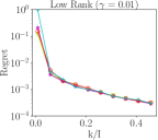
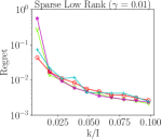
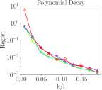
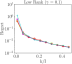
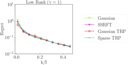
Figure 1: Different DRMs perform similarly. We approximate three-dimensional synthetic tensors (see Section 6.3) with $I=600$, using our one-pass algorithm with $r=5$ and varying $k$ ($s=2k+1$), using different DRMs in the Tucker sketch.

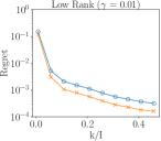
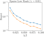
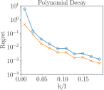
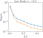
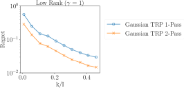
Figure 2: Two-pass improves on one-pass. We approximate three-dimensional synthetic tensors (see Section 6.3) with $I=600$, using our one-pass and two-pass algorithms with $r=5$ and varying $k$ ($s=2k+1$), using the Gaussian TRP in the Tucker sketch.

In this section, we study the performance of our streaming Tucker approximation methods. We compare the performance using various different DRMs, including the TRP. We also compare our method with the algorithm proposed by [31] to show that, for the same storage budget, our method produces better approximations. Our two-pass algorithm outperforms the one-pass version, as expected. (Contrast this to [31], where the multi-pass method performs less well than the one-pass version.)

6.1 Error metrics

We measure the quality of an approximation $\hat{\bm{\mathscr{{X}}}}$ to the original tensor $\bm{\mathscr{{X}}}$ using two different metrics. One is the relative error:

$$\mbox{relative error:}\qquad\|\bm{\mathscr{{X}}}-\hat{\bm{\mathscr{{X}}}}\|_{F}/\|\bm{\mathscr{{X}}}\|_{F}.$$

However, many tensors are not close to low rank, in which case every low-rank approximation will incur high relative error.

Our methods cannot solve the problem that many tensors are not low rank; instead, our goal is just to propose a faster, cheaper, more memory-efficient method to compute a low-rank approximation to the tensor that is almost as good as one computed using a more expensive method like the HOOI, HOSVD, or ST-HOSVD. To facilitate comparisons among approximation algorithms, we define another metric that we call regret. We found that the HOOI performs marginally better than the ST-HOSVD approximation on the examples featured in this section. To simplify plots and interpretations, we treat the HOOI as the gold standard, and we define the regret of an approximation relative to the HOOI as

$$\left(\|\bm{\mathscr{{X}}}-\hat{\bm{\mathscr{{X}}}}\|_{F}-\|\bm{\mathscr{{X}}}-\bm{\mathscr{{X}}}_{\text{HOOI}}\|_{F}\right)/\|\bm{\mathscr{{X}}}\|_{F}.$$

The regret measures the increase in error incurred by using the approximation $\hat{\bm{\mathscr{{X}}}}$ rather than $\bm{\mathscr{{X}}}_{\text{HOOI}}$. The regret of HOOI is 0. An approximation with a regret of $.01$ is only 1% worse than HOOI, relative to the norm of the target tensor $\bm{\mathscr{{X}}}$.

6.2 Computational platform

We ran all experiments on a server with 128 Intel Xeon E7-4850 v4 2.10GHz CPU cores and 1056GB memory. All experiments are implemented in Python. We use the default implementations available in the Python package tensorly [27] for tensor algorithms such as the HOOI and ST-HOSVD. Code for the one- and two-pass approximation algorithms is available on Github at https://github.com/udellgroup/tensorsketch, as is the code that generates the experiments in this paper.

6.3 Synthetic experiments

All synthetic experiments use an input tensor with equal side lengths $I$. We consider three different data generation schemes:

• Low-rank noise. Generate a core tensor $\bm{\mathscr{{C}}}\in\mathbb{R}^{r^{N}}$ with entries drawn i.i.d. from the uniform distribution $U(0,1)$. Generate $N$ random matrices $\mathbf{B}_{1},\dots,\mathbf{B}_{N}\in\mathbb{R}^{r\times I}$ with i.i.d. $\mathcal{N}(0,1)$ entries, and let $\mathbf{A}_{1},\dots,\mathbf{A}_{N}\in\mathbb{R}^{r\times I}$ be orthonormal bases for their respective column spaces. Define $\bm{\mathscr{{X}}}^{\natural}=\bm{\mathscr{{C}}}\times_{1}\mathbf{A}_{1}\cdots\times_{N}\mathbf{A}_{N}$ and the noise parameter $\gamma>0$. Generate an input tensor as $\bm{\mathscr{{X}}}=\bm{\mathscr{{X}}}^{\natural}+(\gamma\|\bm{\mathscr{{X}}}^{\natural}\|_{F}/I^{N/2})\bm{\mathscr{{\epsilon}}}$ where the noise $\bm{\mathscr{{\epsilon}}}$ has i.i.d. $\mathcal{N}(0,1)$ entries.

• Sparse low-rank noise. We construct the input tensor $\bm{\mathscr{{X}}}$ as above (low-rank noise), but with sparse factor matrices $\mathbf{A}_{n}$: If $\delta_{n}$ is the sparsity (proportion of nonzero elements) of $\mathbf{A}_{n}$, then the sparsity of the true signal $\bm{\mathscr{{X}}}^{\natural}$ scales as $r^{N}\prod_{n=1}^{N}\delta_{n}$. We use $\delta_{n}=0.2$ unless otherwise specified.

• Polynomial decay. We construct the input tensor $\bm{\mathscr{{X}}}$ as

  $$\bm{\mathscr{{X}}}=\mathop{\textbf{superdiag}}(1,\dots,1,2^{-t},3^{-t},\dots,(I-r)^{-t}).$$

  The first $r$ entries are 1. Recall that $\mathop{\textbf{superdiag}}$ converts a vector to an $N$-dimensional superdiagonal tensor. Our experiments use $t=1$.

Our goal in including the polynomial and sparse setups is to demonstrate that the method performs robustly and reliably even when the distribution of the data is far from ideal for the method. In the polynomial decay setup, the original tensor is not particularly low rank, so even a rather expensive and accurate method (the HOOI) cannot achieve low error; yet Figs. 1, 2, and 3 tell us that the penalty from using our cheaper methods is essentially the same regardless of the data distribution.

6.3.1 Different dimension reduction maps perform similarly

We first investigate the performance of our one-pass fixed-rank algorithm as the sketch size (hence, the required storage) varies for several types of dimension reduction maps. We generate synthetic data as described above with $\mathbf{r}=(5,5,5)$, $I=600$. Fig. 1 shows the error of the rank-$\mathbf{r}$ approximation as a function of the compression factor $k/I$. (Results for other input tensors are presented as Fig. 8 and Fig. 9 in Appendix D.) In general, the performance for different maps are similar, although our theory only guarantees results for the Gaussian map. We see that for all input tensors, the performance of our one-pass algorithm converges to that of HOOI as $k$ increases.

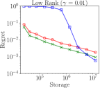
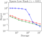
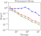
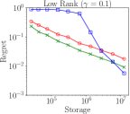
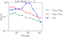
Figure 3: Approximations improve with more memory: synthetic data. We approximate three-dimensional synthetic tensors (see Section 6.3) with $I=300$, using T.-TS and our one-pass and two-pass algorithms with the Gaussian TRP to produce approximations with equal ranks $r=10$. Notice every marker on the plot corresponds to a 2700$\times$ compression!

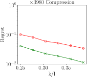
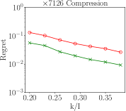
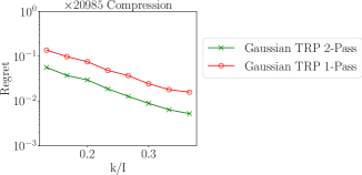
Aerosol Absorption
 

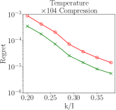
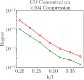
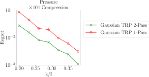
Combustion Simulation

Figure 4: Approximations improve with more memory: real data. We approximate aerosol absorption and combustion data using our one-pass and two-pass algorithms with the Gaussian TRP. We compare three target ranks ($r/I=0.125,0.1,0.067$) for the former, and use the same target rank ($r/I=0.1$) for each measured quantity in the combustion dataset. Notice that $r/I=0.1$ gives a hundred-fold compression. For reference, on the aerosol data, the HOOI gives an approximation with relative errors .23, .26, and .33 for each of the three ranks, respectively; on the combusion data, the relative error of HOOI is .0063, .032, and .28 for temperature, CO, and pressure, respectively.

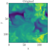
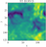
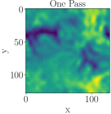
Figure 5: Visualizing combustion simulation: All four figures show a slice of the temperature data along the first dimension. The approximation uses $\mathbf{r}=(281,25,25)$, $\mathbf{k}=(562,50,50)$, $\mathbf{s}=(1125,101,101)$, with the Gaussian TRP in the Tucker sketch.

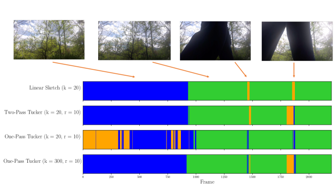
Video scene classification

Figure 6: Video scene classification ($2200\times 1080\times 1980$): We classify frames from the video data from [31] (collected as a third order tensor with size $2200\times 1080\times 1980$) using $K$-means with $K$=3 on vectors computed using four different methods. $s=2k+1$ throughout. (1) The linear sketch along the time dimension (row 1). (2-3) the Tucker factor along the time dimension, computed via our two-pass (row 2) and one-pass (row 3) algorithms. (4) The Tucker factor along the time dimension, computed via our one-pass (row 4) algorithm

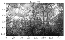
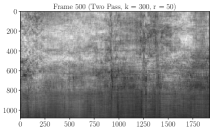
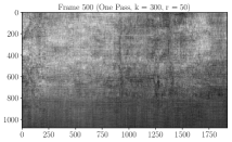
Figure 7: Visualizing video recovery: Original frame (left); approximation by two-pass sketch (middle); approximation by one-pass sketch (right).

6.3.2 A second pass reduces error

The second experiment compares our two-pass and one-pass algorithms. The design is similar to the first experiment. Fig. 2 shows that the two-pass algorithm typically outperforms the one-pass algorithm, especially in the high-noise, sparse, or rank-decay case. Both converge at the same asymptotic rate. (Results for other input tensors are available in Appendix D.)

6.3.3 Improvement on state-of-the-art

The third experiment compares the performance of our two-pass and one-pass algorithms and Tucker TensorSketch (T.–TS), as described in [31], the only extant one-pass algorithm. For a fair comparison, we allocate the same storage budget to each algorithm and compare the relative error of the resulting fixed-rank approximations. We approximate synthetic three-dimensional tensors with equal side lengths $I_{1}=I_{2}=I_{3}=I=300$ and of equal multilinear rank $\mathbf{r}=(r,r,r)$ with $r=10$. We use the suggested parameter settings for each algorithm: $\mathbf{k}=2\mathbf{r}+1$ and $\mathbf{s}=2\mathbf{k}+1$ for our methods; $K=10$ for T.–TS. Our one-pass algorithm (with the Gaussian TRP) uses $((4k+3)^{N}+(2r+1)IN)$ storage, whereas T.-TS uses $(Kr^{2N}+Kr^{2N-2})$ storage (see Table 3 in Appendix C).

Fig. 3 shows that our algorithms generally perform as well as T.–TS and dramatically outperform for small storage budgets. One nice property of our method is that the regret consistently decreases with increasing storage. In contrast, the tensor sketch method behaves unpredictably as storage increases: there are wide plateaus where increasing storage hardly helps at all, and occasionally, increasing storage hurts performance. The performance of T.-TS is comparable with that of the algorithms presented in this paper only when the storage budget is large.

Remark 6.1.

The paper [31] proposes a multi-pass method, Tucker Tensor-Times-Matrix-TensorSketch (TTMTS) that is dominated by the one-pass method Tucker TensorSketch(TS) in all numerical experiments; hence we compare only with T.-TS.

6.4 Applications

We also apply our method to datasets drawn from three application domains: climate, combustion, and video.

• Climate data. We consider global climate simulation datasets from the Community Earth System Model (CESM) Community Atmosphere Model (CAM) 5.0 [22, 23]. The dataset on aerosol absorption has four dimensions: times, altitudes, longitudes, and latitudes ($240\times 30\times 192\times 288$). The data on net radiative flux at surface and dust aerosol burden have three dimensions: times, longitudes, and latitudes ($1200\times 192\times 288$). Each of these quantitives has a strong impact on the absorption of solar radiation and on cloud formation.

• Combustion data. We consider combustion simulation data from [28]. The data consists of three measured quantities (pressure, CO concentration, and temperature) each observed on a $1408\times 128\times 128$ spatial grid.

• Video data. Consider the three-dimensional tensor from [31]: each slice of the tensor is a video frame. A low frame rate camera is mounted in a fixed position as people walk by to form the video, which consists of 2493 frames, each of size 1080 by 1980. Stored as a numpy.array, the video data is 41.4 GB in total.

6.4.1 Data compression

We show that our proposed algorithms are able to successfully compress climate and combustion data even when the full data does not fit in memory. Since the multilinear rank of the original tensor is unknown, we perform experiments for three different target ranks. In this experiment, we hope to understand the effect of different choices of storage budget $k$ to achieve the same compression ratio. We define the compression ratio as the ratio in size between the original input tensor and the output Tucker factors, i.e. $\frac{\prod_{i=1}^{N}I_{i}}{\sum_{i=1}^{N}r_{i}I_{i}+\prod_{i=1}^{N}r_{i}}$. As in our experiments on simulated data, Fig. 4 shows that the two-pass algorithm outperforms the one-pass algorithm as expected. However, as the storage budget $k$ increases, both methods converge to the performance of HOOI. The rate of convergence is faster for smaller target ranks. Performance of our algorithms on the combustion simulation is qualitatively similar but converges faster to the performance of HOOI. Fig. 5 visualizes the recovery of the temperature data in combustion simulation for a slice along the first dimension. We observe that the recovery for both two-pass and one-pass algorithms approximate the recovery from HOOI. Fig. 12 in Fig. 11 shows similar results on another dataset.

6.4.2 Video scene classification

We show how to use our single-pass method to classify scenes in the video data described above. The goal is to identify frames in which people appear. We remove the first 100 frames and last 193 frames where the camera setup happened, as in [31]. We stream over the tensor and sketch it using parameters $k=300,s=601$. Finally, we compute a fixed-rank approximation with $\mathbf{r}=(10,10,10)$ and $(20,20,20)$. We apply K-means clustering to the resulting 10- or 20-dimensional vectors corresponding to each of the remaining 2200 frames.

We experimented with clustering vectors found in three ways: from the unfolding along the time dimension after two-pass or one-pass Tucker approximations, or directly from the factor sketch along the time dimension, which we call the linear sketch. In Fig. 6, comparing the video frames with the classification results, we can see that the background lighting is relatively dark at the beginning, and initial frames are classified into Class $0$. After a change in the background lighting, most other frames of the video are classified into Class $1$. When a person passes by the camera, the frames are classified into Class $2$. Right after the person passes by, the frames are classified into Class $0$, the brighter background scene, due to the light adjustment.

Our classification results (using the linear sketch or approximation) are similar to those in [31] while using only $1/500$ as much storage; the one-pass approximation requires more storage (but still less than [31]) to achieve similar performance. In particular, using the sketch itself, rather than the Tucker approximation, to summarize the data enables very efficient video scene classification. Interestingly, classification works well even though the video is not very low rank along the spatial dimensions. Fig. 7 shows that the scene is poorly approximated even with $\mathbf{s}={601,601,601}$, $\mathbf{k}=(300,300,300)$, and $\mathbf{r}=(50,50,50)$.

Appendix A Probabilistic Analysis of Core Sketch Error

This section contains the most technical part of our proof. We provide a probabilistic error bound for the difference between the two-pass core approximation $\bm{\mathscr{{W}}}_{2}$ from Algorithm 4 and the one-pass core approximation $\bm{\mathscr{{W}}}_{1}$ from Algorithm 5.

Introduce for each $n\in[N]$ the orthonormal matrix $\mathbf{Q}_{n}^{\bot}$ that forms a basis for the subspace orthogonal to $\mathbf{Q}_{n}$, so that $\mathbf{Q}_{n}^{\bot}(\mathbf{Q}_{n}^{\bot})^{\top}=\mathbf{I}-\mathbf{Q}_{n}\mathbf{Q}_{n}^{\top}$. Next, define

(A.1) $$\mathbf{\Phi}_{n}^{Q}=\mathbf{\Phi}^{\top}_{n}\mathbf{Q}_{n},~{}~{}~{}~{}\mathbf{\Phi}_{n}^{Q^{\bot}}=\mathbf{\Phi}^{\top}_{n}\mathbf{Q}_{n}^{\bot}.$$

Recall that the DRMs $\mathbf{\Phi}_{n}$ are i.i.d. Gaussian. Thus, conditional on $\mathbf{Q}_{n}$, the random matrices $\mathbf{\Phi}_{n}^{Q}$ and $\mathbf{\Phi}_{n}^{Q^{\bot}}$ are statistically independent.

A.1 Decomposition of Core Approximation Error

In this section, we characterize the difference between the one- and two-pass core approximations $\bm{\mathscr{{W}}}_{1}-\bm{\mathscr{{W}}}_{2}=\bm{\mathscr{{W}}}_{1}-\bm{\mathscr{{X}}}\times_{1}\mathbf{Q}_{1}^{\top}\dots\times_{N}\mathbf{Q}_{N}^{\top}$.

Lemma 1.

Suppose that $\mathbf{\Phi}_{n}$ has full column rank for each $n\in[N]$. We define $\mathbbm{1}_{a=b}=1$ if $a=b$ and 0 otherwise. Then

$$\bm{\mathscr{{W}}}_{1}-\bm{\mathscr{{W}}}_{2}=\bm{\mathscr{{W}}}_{1}-\bm{\mathscr{{X}}}\times_{1}\mathbf{Q}_{1}^{\top}\dots\times_{N}\mathbf{Q}_{N}^{\top}=\sum_{(i_{1},\dots,i_{N})\in\{0,1\}^{N},\sum_{j=1}^{N}i_{j}\geq 1}\bm{\mathscr{{Y}}}_{i_{1}\dots i_{N}},$$

where

(A.2) $$\bm{\mathscr{{Y}}}_{i_{1}\dots i_{N}} =\bm{\mathscr{{X}}}\times_{1}\left(\mathbbm{1}_{i_{1}=0}\mathbf{Q}_{1}^{\top}+\mathbbm{1}_{i_{1}=1}(\mathbf{\Phi}_{1}^{Q_{1}})^{\dagger}\mathbf{\Phi}_{1}^{Q_{1}^{\bot}}(\mathbf{Q}_{1}^{\bot})^{\top}\right)$$

$$\times_{2}\cdots\times_{N}\left(\mathbbm{1}_{i_{N}=0}\mathbf{Q}_{N}^{\top}+\mathbbm{1}_{i_{1}=1}(\mathbf{\Phi}_{N}^{Q_{N}})^{\dagger}\mathbf{\Phi}_{N}^{Q_{N}^{\bot}}(\mathbf{Q}_{N}^{\bot})^{\top}\right).$$

Proof A.1.

Let $\bm{\mathscr{{H}}}$ be the core sketch from Algorithm 3. Write $\bm{\mathscr{{W}}}_{1}$ as

$$\bm{\mathscr{{W}}}_{1} =\bm{\mathscr{{H}}}\times_{1}(\mathbf{\Phi}_{1}^{\top}\mathbf{Q}_{1})^{\dagger}\times_{2}\cdots\times_{N}(\mathbf{\Phi}^{\top}_{N}\mathbf{Q}_{N})^{\dagger}$$

$$=(\bm{\mathscr{{X}}}-\hat{\bm{\mathscr{{X}}}}_{2})\times_{1}\mathbf{\Phi}^{\top}_{1}\times_{2}\cdots\times_{N}\mathbf{\Phi}^{\top}_{N}\times_{1}(\mathbf{\Phi}^{\top}_{1}\mathbf{Q}_{1})^{\dagger}\times_{2}\cdots\times_{N}(\mathbf{\Phi}^{\top}_{N}\mathbf{Q}_{N})^{\dagger}$$

$$+\hat{\bm{\mathscr{{X}}}}_{2}\times_{1}\mathbf{\Phi}^{\top}_{1}\times_{2}\cdots\times_{N}\mathbf{\Phi}^{\top}_{N}\times_{1}(\mathbf{\Phi}^{\top}_{1}\mathbf{Q}_{1})^{\dagger}\times_{2}\cdots\times_{N}(\mathbf{\Phi}^{\top}_{N}\mathbf{Q}_{N})^{\dagger}.$$

Using the fact that $(\mathbf{\Phi}^{\top}_{n}\mathbf{Q}_{n})^{\dagger}(\mathbf{\Phi}^{\top}_{n}\mathbf{Q}_{n})=\mathbf{I}$, we can simplify the second term as

$$\hat{\bm{\mathscr{{X}}}}_{2}\times_{1}\mathbf{\Phi}^{\top}_{1}\times_{2}\cdots\times_{N}\mathbf{\Phi}^{\top}_{N}\times_{1}(\mathbf{\Phi}^{\top}_{1}\mathbf{Q}_{1})^{\dagger}\times_{2}\cdots\times_{N}(\mathbf{\Phi}^{\top}_{N}\mathbf{Q}_{N})^{\dagger}$$

$$=\bm{\mathscr{{X}}}\times_{1}(\mathbf{\Phi}^{\top}_{1}\mathbf{Q}_{1})^{\dagger}\mathbf{\Phi}^{\top}_{1}\mathbf{Q}_{1}\mathbf{Q}_{1}^{\top}\times_{2}\cdots\times_{N}(\mathbf{\Phi}_{N}^{\top}\mathbf{Q}_{N})^{\dagger}\mathbf{\Phi}_{N}^{\top}\mathbf{Q}_{N}\mathbf{Q}_{N}^{\top}$$

$$=\bm{\mathscr{{X}}}\times_{1}\mathbf{Q}_{1}^{\top}\times_{2}\cdots\times_{N}\mathbf{Q}_{N}^{\top},$$

which is exactly the two-pass core approximation $\bm{\mathscr{{W}}}_{2}$. Therefore

$$\bm{\mathscr{{W}}}_{1}-\bm{\mathscr{{W}}}_{2}=(\bm{\mathscr{{X}}}-\hat{\bm{\mathscr{{X}}}}_{2})\times_{1}\mathbf{\Phi}^{\top}_{1}\times_{2}\cdots\times_{N}\mathbf{\Phi}^{\top}_{N}\times_{1}(\mathbf{\Phi}^{\top}_{1}\mathbf{Q}_{1})^{\dagger}\times_{2}\cdots\times_{N}(\mathbf{\Phi}^{\top}_{N}\mathbf{Q}_{N})^{\dagger}.$$

We continue to simplify this difference:

(A.3) $$(\bm{\mathscr{{X}}}-\tilde{\bm{\mathscr{{X}}}}) \times_{1}\mathbf{\Phi}^{\top}_{1}\times_{2}\cdots\times_{N}\mathbf{\Phi}^{\top}_{N}\times_{1}(\mathbf{\Phi}^{\top}_{1}\mathbf{Q}_{1})^{\dagger}\times_{2}\cdots\times_{N}(\mathbf{\Phi}^{\top}_{N}\mathbf{Q}_{N})^{\dagger}$$

$$=(\bm{\mathscr{{X}}}-\tilde{\bm{\mathscr{{X}}}})\times_{1}(\mathbf{\Phi}^{\top}_{1}\mathbf{Q}_{1})^{\dagger}\mathbf{\Phi}^{\top}_{1}\times_{2}\cdots\times_{N}(\mathbf{\Phi}^{\top}_{N}\mathbf{Q}_{N})^{\dagger}\mathbf{\Phi}_{N}^{\top}$$

$$=(\bm{\mathscr{{X}}}-\tilde{\bm{\mathscr{{X}}}})\times_{1}(\mathbf{\Phi}^{\top}_{1}\mathbf{Q}_{1})^{\dagger}\mathbf{\Phi}^{\top}_{1}(\mathbf{Q}_{1}\mathbf{Q}_{1}^{\top}+\mathbf{Q}_{1}^{\bot}(\mathbf{Q}_{1}^{\bot})^{\top})\dots$$

$$\times_{N}(\mathbf{\Phi}^{\top}_{N}\mathbf{Q}_{N})^{\dagger}\mathbf{\Phi}^{\top}_{N}(\mathbf{Q}_{N}\mathbf{Q}_{N}^{\top}+\mathbf{Q}_{N}^{\bot}(\mathbf{Q}_{N}^{\bot})^{\top})$$

$$=(\bm{\mathscr{{X}}}-\tilde{\bm{\mathscr{{X}}}})\times_{1}(\mathbf{Q}_{1}^{\top}+(\mathbf{\Phi}_{1}^{Q})^{\dagger}\mathbf{\Phi}_{1}^{Q^{\bot}}(\mathbf{Q}_{1}^{\bot})^{\top})\times_{2}\dots$$

$$\times_{N}(\mathbf{Q}_{N}^{\top}+(\mathbf{\Phi}_{N}^{Q_{N}})^{\dagger}\mathbf{\Phi}_{N}^{Q_{N}^{\bot}}(\mathbf{Q}_{N}^{\bot})^{\top}).$$

Many terms in this sum are zero. We use the following two facts:

1. $(\bm{\mathscr{{X}}}-\tilde{\bm{\mathscr{{X}}}})\times_{1}\mathbf{Q}_{1}^{\top}\dots\times_{N}\mathbf{Q}_{N}^{\top}=0$.

2. For each $n\in[N]$, $\tilde{\bm{\mathscr{{X}}}}\times_{n}(\mathbf{\Phi}_{n}^{Q_{n}})^{\dagger}\mathbf{\Phi}_{n}^{Q_{n}^{\bot}}(\mathbf{Q}_{n}^{\bot})^{\top}=0$.

Here, $0$ denotes a tensor with all zero elements. These facts can be obtained from the exchange rule of the mode product and the orthogonality between $\mathbf{Q}_{n}^{\bot}$ and $\mathbf{Q}_{n}$. Using these two facts, we find that only the terms $\bm{\mathscr{{Y}}}_{i_{1}\dots i_{N}}$ (defined in (A.2)) remain in the expression. Therefore, to complete the proof, we write (A.3) as

$$\sum_{(i_{1},\dots,i_{N})\in\{0,1\}^{N},\sum_{n=1}^{N}i_{n}\neq 0}\bm{\mathscr{{Y}}}_{i_{1}\dots i_{N}}.$$

A.2 Probabilistic Core Error Bound

In this section, we derive a probabilistic error bound based on the core error decomposition from 1.

Lemma 2.

Sketch the tensor $\bm{\mathscr{{X}}}$ using a Tucker sketch with parameters $\mathbf{k}$ and $\mathbf{s}>2\mathbf{k}$ with i.i.d. Gaussian $\mathcal{N}(0,1)$ DRMs. Define $\Delta=\max_{n=1}^{N}\frac{k_{n}}{s_{n}-k_{n}-1}$. Let $\hat{\bm{\mathscr{{X}}}_{2}}$ be the output from the two-pass low-rank approximation method (Algorithm 4). Then

(A.4) $$\mathbb{E}\|\bm{\mathscr{{W}}}_{1}-\bm{\mathscr{{X}}}\times_{1}\mathbf{Q}_{1}^{\top}\dots\times_{N}\mathbf{Q}_{N}^{\top}\|_{F}^{2}\leq\Delta\|\bm{\mathscr{{X}}}-\hat{\bm{\mathscr{{X}}}}_{2}\|$$

Proof A.2.

We use the fact that the core DRMs $\{\mathbf{\Omega}_{n}\}_{n\in[N]}$ are independent of the factor matrix DRMs $\{\mathbf{\Phi}_{n}\}_{n\in[N]}$, and that the randomness in each factor matrix approximation $\mathbf{Q}_{n}$ comes solely from $\mathbf{\Omega}_{n}$.

For $i\in\{0,1\}^{N}$, define $\bm{\mathscr{{B}}}_{i_{1}\dots i_{N}}=$

$$\bm{\mathscr{{X}}}\times_{1}(\mathbbm{1}_{i_{1}=0}\mathbf{Q}_{1}\mathbf{Q}_{1}^{\top}+\mathbbm{1}_{i_{1}=1}\mathbf{Q}_{1}^{\bot}(\mathbf{Q}_{1}^{\bot})^{\top})\cdots\times_{N}(\mathbbm{1}_{i_{N}=0}\mathbf{Q}_{N}\mathbf{Q}_{N}^{\top}+\mathbbm{1}_{i_{N}=1}\mathbf{Q}_{N}^{\bot}(\mathbf{Q}_{N}^{\bot})^{\top}).$$

1 decomposes the core error as the sum of $\bm{\mathscr{{Y}}}_{i_{1}\cdots i_{n}}$ where $\sum_{n=1}^{N}i_{n}\geq 1$. Applying 1 and using the orthogonal invariance of the Frobenius norm, we observe

$$\mathbb{E}\left[\|\bm{\mathscr{{Y}}}_{i_{1}\dots i_{N}}\|_{F}^{2}\mid\mathbf{\Omega}_{1}\cdots\mathbf{\Omega}_{N}\right]=\left(\prod_{n=1}^{N}\Delta_{n}^{i_{n}}\right)\|\bm{\mathscr{{B}}}_{i_{1}\dots i_{N}}\|_{F}^{2}\leq\Delta\|\bm{\mathscr{{B}}}_{i_{1}\dots i_{N}}\|_{F}^{2}$$

when $\sum_{n=1}^{N}i_{n}\geq 1$, where $\Delta_{n}=\frac{k_{n}}{s_{n}-k_{n}-1}<1$ and $\Delta=\max_{n=1}^{N}\Delta_{n}$.

Suppose $\mathbf{q}_{1},\mathbf{q}_{2}\in\{0,1\}^{N}$ are index (binary) vectors of length $N$. For different indices $\mathbf{q}_{1}$ and $\mathbf{q}_{2}$, there exists some $1\leq r\leq N$ such that their $r$th element is different. Without loss of generality, assume $\mathbf{q}_{1}(r)=0$ and $\mathbf{q}_{2}(r)=1$ to see

(A.5) $$\langle\bm{\mathscr{{B}}}_{q_{1}},\bm{\mathscr{{B}}}_{q_{2}}\rangle=\langle\dots\mathbf{Q}_{r}^{\top}\mathbf{Q}_{r}^{\bot}\dots\rangle=0.$$

Similarly we can show that the inner product between $\bm{\mathscr{{Y}}}_{q_{1}}$ and $\bm{\mathscr{{Y}}}_{q_{2}}$ is zero with different $\mathbf{q}_{1},\mathbf{q}_{2}$. Noticing that $\bm{\mathscr{{B}}}_{0,\ldots,0}=\hat{\bm{\mathscr{{X}}}}_{2}$, we have

$$\|\bm{\mathscr{{X}}}-\hat{\bm{\mathscr{{X}}}}_{2}\|_{F}^{2} =\left\|\sum_{(i_{1},\dots,i_{N})\in\{0,1\}^{N},\sum_{n=1}^{N}i_{n}\geq 1}\bm{\mathscr{{B}}}_{i_{1}\dots i_{N}}\right\|_{F}^{2} =\sum_{\begin{subarray}{c}(i_{1},\dots,i_{N})\in\{0,1\}^{N},\\ \sum_{n=1}^{N}i_{n}\geq 1\end{subarray}}\|\bm{\mathscr{{B}}}_{i_{1}\dots i_{N}}\|_{F}^{2}.$$

Put these together and use the Pythagorean theorem to finish the proof:

$$\mathbb{E}\left[\|\bm{\mathscr{{W}}}-\bm{\mathscr{{X}}}\times_{1}\mathbf{Q}_{1}^{\top}\dots\times_{N}\mathbf{Q}_{N}^{\top}\|_{F}^{2}\mid\mathbf{\Omega}_{1},\cdots,\mathbf{\Omega}_{N}\right]$$

$$=\sum_{(i_{1},\dots,i_{N})\in\{0,1\}^{N},\sum_{n=1}^{N}i_{n}\geq 1}\mathbb{E}\left[\|\bm{\mathscr{{Y}}}_{i_{1}\dots i_{N}}\|_{F}^{2}\mid\mathbf{\Omega_{1}},\dots,\mathbf{\Omega}_{N}\right]$$

$$\leq\Delta\left(\sum_{(i_{1},\dots,i_{N})\in\{0,1\}^{N},\sum_{n=1}^{N}i_{n}\geq 1}\|\bm{\mathscr{{B}}}_{i_{1}\dots i_{N}}\|_{F}^{2}\right)=\Delta\|\bm{\mathscr{{X}}}-\hat{\bm{\mathscr{{X}}}}_{2}\|_{F}^{2}.$$

Appendix B Random matrix projections

Proofs for the lemmas in this section can be found in [21, sections 9 and 10].

Lemma 1.

Assume that $t>q$. Suppose $\mathbf{G}_{1}\in\mathbb{R}^{t\times q}$ and $\mathbf{G}_{2}\in\mathbb{R}^{t\times p}$ have i.i.d. standard normal entries. For any matrix $\mathbf{B}$ with conforming dimensions,

$$\mathbb{E}\|\mathbf{G}_{1}^{\dagger}\mathbf{G}_{2}\mathbf{B}\|_{F}^{2}=\frac{q}{t-q-1}\|\mathbf{B}\|_{F}^{2}.$$

Lemma 2.

Given a fixed $\mathbf{A}\in\mathbb{R}^{m\times n}$ and random $\mathbf{\Omega}\in\mathbb{R}^{n\times k}$ with i.i.d. standard normal entries, let $\mathbf{Q}_{\rho}=\textup{TruncatedQR}(\mathbf{A\Omega},\rho)\in\in\mathbb{R}^{n\times\rho}$ for $\rho<k-1$ [19]. Then

(B.1) $$\mathbb{E}\|(\mathbf{I}-\mathbf{Q_{\rho}Q_{\rho}^{\top}})\mathbf{A}\|_{F}^{2}\leq\frac{\rho}{k-\rho-1}\tau_{\rho}.$$

Corollary B.1.

Under the same conditions as in 2, suppose $\mathbf{Q}=\textup{QR}(\mathbf{A\Omega})$ is an orthogonal matrix spanning the column space of $\mathbf{A\Omega}$. Then

(B.2) $$\mathbb{E}\|(\mathbf{I}-\mathbf{QQ^{\top}})\mathbf{A}\|_{F}^{2}\leq\min_{1\leq\rho<k-1}\frac{\rho}{k-\rho-1}\tau_{\rho}.$$

Proof B.2.

For each $\rho<k-1$,

$$\|(\mathbf{I}-\mathbf{Q_{\rho}Q_{\rho}^{\top}})\mathbf{A}\|_{F}^{2}\leq\|(\mathbf{I}-\mathbf{Q_{\rho}Q_{\rho}^{\top}})\mathbf{A}\|_{F}^{2}\leq\frac{r}{k-\rho-1}\tau_{\rho},$$

using Eq. B.1 for the second inequality. Minimize over $\rho<k-1$ to reach the result.

Appendix C Time and Storage Complexity

C.1 Comparison Between Algorithm 6 and T.-TS [31]

Here we compare the time and storage complexity of the two extant methods for streaming Tucker approximation: our one-pass method, and T.-TS [31].

To compare the storage and time costs of both T.-TS and the one-pass algorithm, we separate the cost into two parts: one for forming the sketch, the other for each iteration of ALS. Assume the tensor to approximate has equal side lengths $I_{1}=\cdots=I_{N}=I$ and that the target rank for each mode is $R$.

The suggested default parameters for the sketch in [31] are $J_{1}=10R^{N-1}$ and $J_{2}=10R^{N}$. Our suggested default parameters are $k=2r,s=2k+1$. Under the choice of the default parameter, we compare the the cost of storage and time in Table 3 and Table 4. In most problems with data that is not exactly low rank, i.e. $R>4$, the suggested default setting of T.-TS typically leads to a higher storage cost. Moreover, our algorithm uses less storage and is faster to compute, particularly for tensors with many modes $N$.

However, the evaluation of the two algorithms should not be solely based on their default setups. If the memory constraint is set to be the same, our one-pass algorithm performs much better in the low-memory case, but slightly worse in the high-memory case (see Fig. 3). The memory required by our default parameters is typically much smaller than that required with the default parameters of [31].

C.2 Computational Complexity of Algorithm 6

Here, we will calculate the computational complexity for our one-pass fixed-rank approximation algorithm.

In the sketching stage of the streaming algorithm, we first need to compute the factor sketches, $\mathbf{G}_{n}=\mathbf{X}\mathbf{\Omega}_{n},n\in[N]$ with $kN\hat{I}$ flops in total. Then we need to compute the core tensor sketch $\mathscr{Z}$ by recursively multiplying $\mathscr{X}$ by $\mathbf{\Phi}_{n},n\in[N]$. We can upper bound the number of flops by $\frac{s(1-\delta_{1}^{N})}{1-\delta_{1}}\bar{I}$. Then in the approximation stage, we first perform “economy size” QR factorizations of $\mathbf{G}_{1},\dots,\mathbf{G}_{N}$ with $\mathscr{O}(k^{2}(\sum_{n=1}^{N}I_{n}))$ to find the orthonormal bases $\mathbf{Q}_{1},\dots,\mathbf{Q}_{N}$. To find the linkage tensor $\mathscr{W}$, we need to recursively solve linear square problems with $\frac{k^{2}s^{N}(1-(k/s)^{N})}{1-k/s}$ flops. Overall, the sketch computation dominates the total time complexity.

The HOSVD directly acts on $\mathscr{X}$ by first computing the SVD for each unfolding ($\mathscr{O}(kN\bar{I})$) and then multiplying $\mathscr{X}$ by $\mathbf{U}_{1}^{\top},\dots,\mathbf{U}_{N}^{\top}$ ($\mathcal{O}(\frac{k(1-\delta_{1}^{N})\bar{I}}{1-\delta_{1}})$). The total time cost is less than the streaming algorithm with a constant factor. Note: we can use the randomized SVD in the first step of the HOSVD to improve the computational cost to $\bar{I}N\log k+\sum_{n=1}^{N}(I_{n}+I_{(-n)})k^{2}$ [21].

Algorithm		Storage Cost ($I=o(r^{2N})$)
T.-TS	Sketching	$\mathcal{O}(r^{2N})$
	Recovery	$\mathcal{O}(r^{2N})$
Algorithm 5 (One Pass)	Sketching	$\mathcal{O}(4^{N}r^{N})$
	Recovery	$\mathcal{O}(4^{N}r^{N})$

Table 3: Storage complexity of Algorithm 5 and T.-TS on tensor $\bm{\mathscr{{X}}}\in\mathbb{R}^{I\times\dots\times I}$. Algorithm 5 uses parameters $(k,s)=(2r,4r+1)$ and uses a TRP composed of Gaussian DRMs inside the Tucker sketch. T.-TS uses default values for hyper-parameters: $J_{1}=10r^{N-1},J_{2}=10r^{N}$.

Algorithm		Time Cost ($I=o(r^{2N})$)
T.-TS	Sketching	$\mathcal{O}(N\rm{nnz}(\bm{\mathscr{{X}}}))$
	Recovery	$\mathcal{O}(NIr^{N}+Nr^{2N-1}+r^{2N})$
Algorithm 5 (One Pass)	Sketching	$\mathcal{O}(Nr~{}\rm{nnz}(\bm{\mathscr{{X}}})))$
	Recovery	$\mathcal{O}(Nr^{N+1})$

Table 4: Time complexity of Algorithm 5 and T.-TS on tensor $\bm{\mathscr{{X}}}\in\mathbb{R}^{I\times\dots\times I}$. Algorithm 5 uses parameters $(k,s)=(2r,4r+1)$ and uses a TRP composed of Gaussian DRMs inside the Tucker sketch. T.-TS uses default values for hyper-parameters: $J_{1}=10r^{N-1},J_{2}=10r^{N}$.

Appendix D More Numerics

This section provides more numerical results on simulated datasets in Fig. 8, Fig. 9, Fig. 10, and Fig. 11.

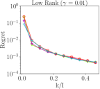
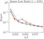
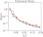
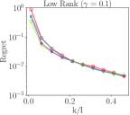
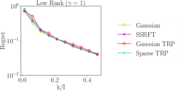
Figure 8: We approximate 3D synthetic tensors (see Section 6.3) with $I=400$, using our one-pass algorithm with $r=5$ and varying $k$ ($s=2k+1$), using a variety of DRMs in the Tucker sketch: Gaussian, SSRFT, Gaussian TRP, or Sparse TRP.

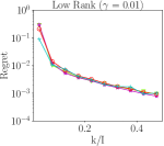
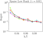
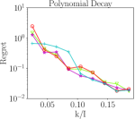
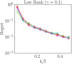
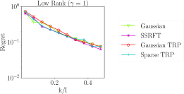
Figure 9: We approximate 3D synthetic tensors (see Section 6.3) with $I=200$, using our one-pass algorithm with $r=5$ and varying $k$ ($s=2k+1$), using a variety of DRMs in the Tucker sketch: Gaussian, SSRFT, Gaussian TRP, or Sparse TRP.

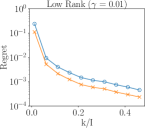
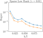
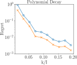
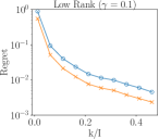
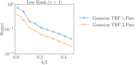
Figure 10: We approximate 3D synthetic tensors (see Section 6.3) with $I=400$, using our one-pass and two-pass algorithms with $r=5$ and varying $k$ ($s=2k+1$), using the Gaussian TRP in the Tucker sketch.

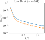
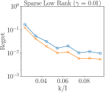
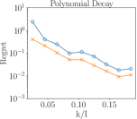
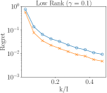
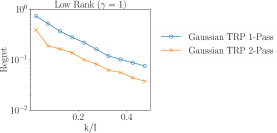
Figure 11: We approximate 3D synthetic tensors (see Section 6.3) with $I=200$, using our one-pass and two-pass algorithms with $r=5$ and varying $k$ ($s=2k+1$), using the Gaussian TRP in the Tucker sketch.

We also provide more numerical results on real datasets in Fig. 12.

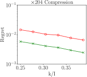
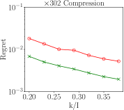
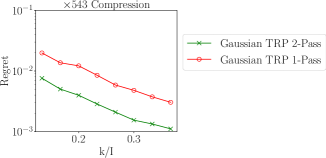
Net Radiative Flux at Surface
 

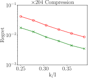
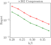
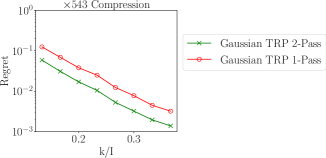
Dust Aerosol Burden

Figure 12: We approximate the net radiative flux and dust aerosol burden data using our one-pass and two-pass algorithms using Gaussian TRP. We compare the performance under different ranks ($r/I=0.125,0.2,0.067$). The dataset comes from the CESM CAM. The dust aerosol burden measures the amount of aerosol contributed by the dust. The net radiative flux determines the energy received by the earth surface through radiation.

Appendix E More Algorithms

This section provides detailed implementations.

Algorithm 7 Higher order orthogonal iteration (HOOI) [14]

Given: tensor $\bm{\mathscr{{X}}}$, target rank $\mathbf{r}=(r_{1},\ldots,r_{N})$
Initialize: compute $\bm{\mathscr{{X}}}\approx\llbracket\bm{\mathscr{{G}}};\mathbf{U}_{1},\ldots,\mathbf{U}_{N}\rrbracket$ using HOSVD
Repeat:

1. Factors. For each $n\in[N]$,

   (E.1) $$\mathbf{U}_{n}\leftarrow\operatorname*{arg\,min}_{\mathbf{U_{n}}}\left\|\llbracket\bm{\mathscr{{G}}};\mathbf{U}_{1},\ldots,\mathbf{U}_{N}\rrbracket-\bm{\mathscr{{X}}}\right\|_{F}^{2},$$

2. Core.

   (E.2) $$\bm{\mathscr{{G}}}\leftarrow\operatorname*{arg\,min}_{\bm{\mathscr{{G}}}}\left\|\llbracket\bm{\mathscr{{G}}};\mathbf{U}_{1},\ldots,\mathbf{U}_{N}\rrbracket-\bm{\mathscr{{X}}}\right\|_{F}^{2}.$$

   $$i.e.~{}~{}\bm{\mathscr{{G}}}=\bm{\mathscr{{X}}}\times_{1}\mathbf{U}_{1}^{\top}\times_{2}\cdots\times_{N}\mathbf{U}_{N}^{\top}$$

Return: Tucker approximation $\bm{\mathscr{{X}}}_{\rm{HOOI}}=\llbracket\bm{\mathscr{{G}}};\mathbf{U}_{1},\ldots,\mathbf{U}_{N}\rrbracket$

Notice the core update (LABEL:eq:core_update) admits the closed form solution $\bm{\mathscr{{G}}}\leftarrow\bm{\mathscr{{X}}}\times_{1}\mathbf{U}_{1}^{\top}\cdots\times_{N}\mathbf{U}_{N}^{\top}$, which motivates the second step of HOSVD for a linear sketch appropriate to a streaming setting (Algorithm 8) or a distributed setting (Algorithm 9).

Algorithm 8 Linear Update to Sketches

1:function SketchLinearUpdate($\bm{\mathscr{{F}}},\mathbf{V}_{1},\dots,\mathbf{V}_{N},\bm{\mathscr{{H}}}$; $\theta_{1}$, $\theta_{2}$)

2:     for $n=1,\dots,N$ do

3:         $\mathbf{V}_{n}\leftarrow\theta_{1}\mathbf{V}_{n}+\theta_{2}\mathbf{F}^{(n)}\mathbf{\Omega}_{n}$

4:     end for

5:     $\bm{\mathscr{{H}}}\leftarrow\theta_{1}\bm{\mathscr{{H}}}+\theta_{2}\bm{\mathscr{{F}}}\times_{1}\mathbf{\Phi}_{1}\times\cdots\times_{N}\mathbf{\Phi}_{N}$

6:     return $(\mathbf{V}_{1},\dots,\mathbf{V}_{N},\bm{\mathscr{{H}}})$

7:end function

1:$\bm{\mathscr{{X}}}_{i}$ is the part of the tensor $\bm{\mathscr{{X}}}$ at local machine $i$ and $\bm{\mathscr{{X}}}=\sum_{i=1}^{m}\bm{\mathscr{{X}}}_{i}$.

2:function ComputeSketchDistributed($\bm{\mathscr{{X}}}_{1},\ldots,\bm{\mathscr{{X}}}_{m}$)

3:     Send the same random generating environment to every local machine.

4:     Generate the same DRM at each local machine.

5:     for $i=1\dots m$ do

6:         $(\mathbf{V}_{1}^{(i)},\cdots,\mathbf{V}_{n}^{(i)},\bm{\mathscr{{H}}}^{(i)})\leftarrow$ ComputeSketch($\bm{\mathscr{{X}}}_{i}$)

7:     end for

8:     for $j=1\dots n$ do

9:         $\mathbf{V}_{j}\leftarrow\sum_{i=1}^{m}\mathbf{V}_{j}^{(i)}$

10:     end for

11:     $\bm{\mathscr{{H}}}\leftarrow\sum_{i=1}^{m}\bm{\mathscr{{H}}}^{(i)}$

12:     return $(\mathbf{V}_{1},\dots,\mathbf{V}_{n},\bm{\mathscr{{H}}})$

13:end function

Algorithm 9 Sketching in Distributed Setting

Appendix F Scrambled Subsampled Randomized Fourier Transform

In order to reduce the cost of storing the test matrices, in particular, $\mathbf{\Omega}_{1},\dots,\mathbf{\Omega}_{N}$, we can use the Scrambled Subsampled Randomized Fourier Transform (SSRFT). To reduce the dimension of a matrix, $\mathbf{X}\in\mathbb{R}^{m\times n}$, along either the row or the column to size $k$, we define the SSRFT map $\mathbf{\Xi}$ as:

$$\mathbf{\Xi}=\begin{cases}\mathbf{R}\mathbf{F}^{\top}\mathbf{\Pi}\mathbf{F}\mathbf{\Pi}^{\top}\in\mathbb{F}^{k\times m}&\text{(Row linear transform)}\\ (\widebar{\mathbf{R}}\widebar{\mathbf{F}}^{\top}\widebar{\mathbf{\Pi}}\widebar{\mathbf{F}}\widebar{\mathbf{\Pi}}^{\top})^{\top}\in\mathbb{F}^{n\times k}&\text{(Column linear transform)},\end{cases}$$

where $\mathbf{\Pi},\mathbf{\Pi}^{\prime}\in\mathbb{R}^{m\times m},\widebar{\mathbf{\Pi}},\widebar{\mathbf{\Pi}}^{\prime}\in\mathbb{R}^{n\times n}$ are signed permutation matrices. That is, the matrix has exactly one non-zero entry, 1 or -1 with equal probability, in each row and column. $\mathbf{F}\in\mathbb{F}^{m\times m},\mathbf{F}\in\mathbb{F}^{n\times n}$ denote the discrete cosine transform ($\mathbb{F}=\mathbb{R}$) or the discrete fourier transform ($\mathbb{F}=\mathbb{C}$). The matrix $\mathbf{R},\widebar{\mathbf{R}}$ is the restriction to $k$ coordinates chosen uniformly at random.

In practice, we implement the SSRFT as in Algorithm 10. It takes only $\mathcal{O}(m)$ or $\mathcal{O}(n)$ bits to store $\mathbf{\Xi}$, compared to $\mathcal{O}(km)$ or $\mathcal{O}(kn)$ for Gaussian or uniform random map. The cost of applying $\mathbf{\Xi}$ to a vector is $\mathcal{O}(n\log n)$ or $\mathcal{O}(m\log m)$ arithmetic operations for fast Fourier transform and $\mathcal{O}(n\log k)$ or $\mathcal{O}(m\log k)$ for fast cosine transform. Though in practice, SSRFT behaves similarly to the Gaussian random map, its analysis is less comprehensive [9, 38, 2] than the Gaussian case.

1:$\mathbf{X}\in\mathbb{R}^{m\times n},\mathcal{F}=\mathbb{R}$, randperm creates a random permutaion vector, and randsign creates a random sign vector. dct denotes the discrete cosine transform.

2:function SSRFT($\mathbf{X}$)

3:     coords $\leftarrow$ randperm(m,k)

4:     $\textbf{perm}_{j}\leftarrow\textbf{randperm}(m)$ for $j=1,2$

5:     $\textbf{sgn}_{j}\leftarrow\textbf{randsign}(m)$ for $j=1,2$

6:     $\mathbf{X}\leftarrow\textbf{dct}(\textbf{sgn}_{1}\cdot\mathbf{X}[\textbf{perm}_{1},:])$ $\triangleright$ elementwise product

7:     $\mathbf{X}\leftarrow\textbf{dct}(\textbf{sgn}_{2}\cdot\mathbf{X}[\textbf{perm}_{2},:])$

8:     return $\mathbf{X}[\textbf{coords},:]$

9:end function

Algorithm 10 Scrambled Subsampled Randomized Fourier Transform (Row Linear Transform)

Appendix G TensorSketch

Many authors have developed methods to perform dimension reduction efficiently. In particular, [17] proposed a method called TensorSketch that aims to solve least squares problems for which the design matrix has a Kronecker product structure. [31] use this technique to compute a one-pass Tucker decomposition. Here we review the TensorSketch and how it is used in [31].

CountSketch

[13] proposed the CountSketch method. A comprehensive theoretical analysis in the context of low-rank approximation problems appears in [12]. To compute the sketch $\mathbf{X}\mathbf{\Omega}\in\mathbb{R}^{d\times k}$ for $\mathbf{X}\in\mathbb{R}^{m\times d}$, CountSketch defines $\mathbf{\Omega}=\mathbf{D}\mathbf{\Phi}$, where

1. $\mathbf{D}\in\mathbb{R}^{d\times d}$ is a diagonal matrix with each diagonal entry equal to $(-1,1)$ with probability $(1/2,1/2)$.

2. $\mathbf{\Phi}\in\mathbb{R}^{d\times k}$ is the matrix form of a hash function.

These two matrices have $2d$ non-zero entries in total and thus require much less storage than the standard $kd$ entries. Furthermore, these two matrices can operate on each column of $\mathbf{X}$ at a cost of only $\mathcal{O}(kd)$ arithmetic operations.

TensorSketch

[31] proposes to use the CountSketch inside the HOOI method for Tucker decomposition They apply the sketch to solve least squares problems appearing in (E.1) and (LABEL:eq:core_update) in Algorithm 7. They use $J_{1},J_{2}$ to denote the reduced dimension. Using a standard random map, it would require a $J_{1}$-by-$I_{(-n)}$ random matrix to solve the problem in Eq. E.1 and a $J_{2}$-by-$\prod_{n=1}^{N}I_{n}$ random matrix to solve the problem in LABEL:eq:core_update. However, these problems have Kronecker problem structure: as shown in [31], these two stages can be expressed as

(G.1) $$\text{For }n=1,\dots,N,\text{update }\mathbf{U}^{(n)}=\underset{\mathbf{U}\in\mathbb{R}^{I_{n}\times R_{n}}}{\arg\min}\left\|\left(\bigotimes_{i=N\atop i\neq n}^{1}\mathbf{U}^{(i)}\right)\mathbf{G}_{(n)}^{\top}\mathbf{U}^{\top}-\mathbf{Y}_{(n)}^{\top}\right\|_{F}^{2}.$$

(G.2) $$\text{Update }\mathcal{G}=\underset{\bm{\mathscr{{Z}}}\in\mathbb{R}^{R_{1}\times\cdots\times R_{N}}}{\arg\min}\left\|\left(\bigotimes_{i=N}^{1}\mathbf{U}^{(i)}\right)\mathop{\mathbf{vec}}{\bm{\mathscr{{Z}}}}-\mathop{\mathbf{vec}}{\bm{\mathscr{{Y}}}}\right\|_{2}^{2},$$

where $\bm{\mathscr{{Y}}}$ is the original data. Here $\forall i\in[n],\mathbf{U}_{i}$ is the factor matrix, and $\bm{\mathscr{{G}}}$ is the core tensor. The target multilinear rank is $(R_{1},\dots,R_{N})$.

Following [17], [31] proposes to apply TensorSketch to the Kronecker product structure of the input matrix in the sketch construction, i.e. $\otimes_{\begin{subarray}{c}i=1\\ i\neq n\end{subarray}}^{N}\mathbf{U}_{i}$ in Eq. G.1 and $\otimes_{i=1}^{N}\mathbf{U}_{i}$ in Eq. G.2. The TensorSketch method combines the CountSketch of each factor matrix via the Khatri-Rao product and Fast Fourier Transform. Consider sketching $\otimes_{i=1}^{N}\mathbf{U}_{i}$ in Eq. G.2. TensorSketch is defined as

(G.3) $$\mathbf{\Omega}\mathbf{X}=\text{FFT}^{-1}\bigg{(}\odot_{n=1}^{N}\Big{(}\text{FFT}\big{(}\text{CountSketch}^{(n)}(\mathbf{U}^{(n)})\big{)}^{\top}\Big{)}^{\top}\bigg{)}$$

By only storing $\text{CountSketch}^{(1)},\dots,\text{CountSketch}^{(N)}$, TensorSketch only requires storage $2\sum_{i=1}^{N}I_{n}$. Therefore, the storage cost of the sketch is dominated by the sketch size, $NR^{n-1}J_{1}+J_{2}R^{n}\approx NKR^{2n-2}+KR^{2n}$, when $J_{1}=KR^{n-1},J_{2}=KR^{n}$.

References

• [1] D. Achlioptas, Database-friendly random projections: Johnson-Lindenstrauss with binary coins, Journal of computer and System Sciences, 66 (2003), pp. 671–687.
• [2] N. Ailon and B. Chazelle, The fast Johnson–Lindenstrauss transform and approximate nearest neighbors, SIAM Journal on computing, 39 (2009), pp. 302–322.
• [3] S. Arora and B. Barak, Computational complexity: a modern approach, Cambridge University Press, 2009.
• [4] W. Austin, G. Ballard, and T. G. Kolda, Parallel tensor compression for large-scale scientific data, in Parallel and Distributed Processing Symposium, 2016 IEEE International, IEEE, 2016, pp. 912–922.
• [5] R. Ballester-Ripoll, P. Lindstrom, and R. Pajarola, TTHRESH: Tensor compression for multidimensional visual data, IEEE transactions on visualization and computer graphics, (2019).
• [6] M. Baskaran, B. Meister, N. Vasilache, and R. Lethin, Efficient and scalable computations with sparse tensors, in High Performance Extreme Computing (HPEC), 2012 IEEE Conference on, IEEE, 2012, pp. 1–6.
• [7] C. Battaglino, G. Ballard, and T. G. Kolda, A practical randomized cp tensor decomposition, SIAM Journal on Matrix Analysis and Applications, 39 (2018), pp. 876–901.
• [8] C. Battaglino, G. Ballard, and T. G. Kolda, Faster parallel tucker tensor decomposition using randomization, (2019).
• [9] C. Boutsidis and A. Gittens, Improved matrix algorithms via the subsampled randomized hadamard transform, SIAM Journal on Matrix Analysis and Applications, 34 (2013), pp. 1301–1340.
• [10] P. Breiding and N. Vannieuwenhoven, A riemannian trust region method for the canonical tensor rank approximation problem, SIAM Journal on Optimization, 28 (2018), pp. 2435–2465.
• [11] A. Cichocki, Tensor decompositions: a new concept in brain data analysis?, arXiv preprint arXiv:1305.0395, (2013).
• [12] K. L. Clarkson and D. P. Woodruff, Low-rank approximation and regression in input sparsity time, Journal of the ACM (JACM), 63 (2017), p. 54.
• [13] G. Cormode and M. Hadjieleftheriou, Finding frequent items in data streams, Proceedings of the VLDB Endowment, 1 (2008), pp. 1530–1541.
• [14] L. De Lathauwer, B. De Moor, and J. Vandewalle, A multilinear singular value decomposition, SIAM journal on Matrix Analysis and Applications, 21 (2000), pp. 1253–1278.
• [15] L. De Lathauwer, B. De Moor, and J. Vandewalle, On the best rank-1 and rank-(r1, r2, …, rn) approximation of higher-order tensors, SIAM Journal on Matrix Analysis and Applications, 21 (2000), pp. 1324–1342, https://doi.org/10.1137/S0895479898346995, https://doi.org/10.1137/S0895479898346995, https://arxiv.org/abs/https://doi.org/10.1137/S0895479898346995.
• [16] V. De Silva and L.-H. Lim, Tensor rank and the ill-posedness of the best low-rank approximation problem, SIAM Journal on Matrix Analysis and Applications, 30 (2008), pp. 1084–1127.
• [17] H. Diao, Z. Song, W. Sun, and D. P. Woodruff, Sketching for Kronecker Product Regression and P-splines, arXiv e-prints, (2017), arXiv:1712.09473, p. arXiv:1712.09473, https://arxiv.org/abs/1712.09473.
• [18] L. Grasedyck, Hierarchical singular value decomposition of tensors, SIAM Journal on Matrix Analysis and Applications, 31 (2010), pp. 2029–2054.
• [19] M. Gu and S. C. Eisenstat, Efficient algorithms for computing a strong rank-revealing qr factorization, SIAM Journal on Scientific Computing, 17 (1996), pp. 848–869.
• [20] W. Hackbusch, Tensor spaces and numerical tensor calculus, vol. 42, Springer Science & Business Media, 2012.
• [21] N. Halko, P.-G. Martinsson, and J. A. Tropp, Finding structure with randomness: Probabilistic algorithms for constructing approximate matrix decompositions, SIAM review, 53 (2011), pp. 217–288.
• [22] J. W. Hurrell, M. M. Holland, P. R. Gent, S. Ghan, J. E. Kay, P. J. Kushner, J.-F. Lamarque, W. G. Large, D. Lawrence, K. Lindsay, et al., The community earth system model: a framework for collaborative research, Bulletin of the American Meteorological Society, 94 (2013), pp. 1339–1360.
• [23] J. Kay, C. Deser, A. Phillips, A. Mai, C. Hannay, G. Strand, J. Arblaster, S. Bates, G. Danabasoglu, J. Edwards, et al., The community earth system model (cesm) large ensemble project: A community resource for studying climate change in the presence of internal climate variability, Bulletin of the American Meteorological Society, 96 (2015), pp. 1333–1349.
• [24] O. Kaya and B. Uçar, High performance parallel algorithms for the tucker decomposition of sparse tensors, in Parallel Processing (ICPP), 2016 45th International Conference on, IEEE, 2016, pp. 103–112.
• [25] T. G. Kolda and B. W. Bader, Tensor decompositions and applications, SIAM review, 51 (2009), pp. 455–500.
• [26] T. G. Kolda and J. Sun, Scalable tensor decompositions for multi-aspect data mining, in 2008 Eighth IEEE International Conference on Data Mining, IEEE, 2008, pp. 363–372.
• [27] J. Kossaifi, Y. Panagakis, A. Anandkumar, and M. Pantic, Tensorly: Tensor learning in python, The Journal of Machine Learning Research, 20 (2019), pp. 925–930.
• [28] S. Lapointe, B. Savard, and G. Blanquart, Differential diffusion effects, distributed burning, and local extinctions in high karlovitz premixed flames, Combustion and flame, 162 (2015), pp. 3341–3355.
• [29] J. Li, C. Battaglino, I. Perros, J. Sun, and R. Vuduc, An input-adaptive and in-place approach to dense tensor-times-matrix multiply, in High Performance Computing, Networking, Storage and Analysis, 2015 SC-International Conference for, IEEE, 2015, pp. 1–12.
• [30] P. Li, T. J. Hastie, and K. W. Church, Very sparse random projections, in Proceedings of the 12th ACM SIGKDD international conference on Knowledge discovery and data mining, ACM, 2006, pp. 287–296.
• [31] O. A. Malik and S. Becker, Low-rank tucker decomposition of large tensors using tensorsketch, in Advances in Neural Information Processing Systems, 2018, pp. 10116–10126.
• [32] R. Minster, A. K. Saibaba, and M. E. Kilmer, Randomized algorithms for low-rank tensor decompositions in the tucker format, arXiv preprint arXiv:1905.07311, (2019).
• [33] S. Muthukrishnan et al., Data streams: Algorithms and applications, Foundations and Trends® in Theoretical Computer Science, 1 (2005), pp. 117–236.
• [34] S. Oymak and J. A. Tropp, Universality laws for randomized dimension reduction, with applications, Information and Inference: A Journal of the IMA, (2015).
• [35] M. Rudelson, Row products of random matrices, Advances in Mathematics, 231 (2012), pp. 3199–3231.
• [36] J. Sun, D. Tao, S. Papadimitriou, P. S. Yu, and C. Faloutsos, Incremental tensor analysis: Theory and applications, ACM Transactions on Knowledge Discovery from Data (TKDD), 2 (2008), p. 11.
• [37] Y. Sun, Y. Guo, J. A. Tropp, and M. Udell, Tensor random projection for low memory dimension reduction, in NeurIPS Workshop on Relational Representation Learning, 2018, https://r2learning.github.io/assets/papers/CameraReadySubmission%2041.pdf.
• [38] J. A. Tropp, Improved analysis of the subsampled randomized hadamard transform, Advances in Adaptive Data Analysis, 3 (2011), pp. 115–126.
• [39] J. A. Tropp, A. Yurtsever, M. Udell, and V. Cevher, Practical sketching algorithms for low-rank matrix approximation, SIAM Journal on Matrix Analysis and Applications, 38 (2017), pp. 1454–1485.
• [40] J. A. Tropp, A. Yurtsever, M. Udell, and V. Cevher, More practical sketching algorithms for low-rank matrix approximation, Tech. Report 2018-01, California Institute of Technology, Pasadena, California, 2018.
• [41] J. A. Tropp, A. Yurtsever, M. Udell, and V. Cevher, Streaming low-rank matrix approximation with an application to scientific simulation, SIAM Journal on Scientific Computing (SISC), (2019), https://arxiv.org/abs/1902.08651.
• [42] C. E. Tsourakakis, Mach: Fast randomized tensor decompositions, in Proceedings of the 2010 SIAM International Conference on Data Mining, SIAM, 2010, pp. 689–700.
• [43] L. R. Tucker, Some mathematical notes on three-mode factor analysis, Psychometrika, 31 (1966), pp. 279–311.
• [44] N. Vannieuwenhoven, R. Vandebril, and K. Meerbergen, A new truncation strategy for the higher-order singular value decomposition, SIAM Journal on Scientific Computing, 34 (2012), pp. A1027–A1052.
• [45] M. A. O. Vasilescu and D. Terzopoulos, Multilinear analysis of image ensembles: Tensorfaces, in European Conference on Computer Vision, Springer, 2002, pp. 447–460.
• [46] Y. Wang, H.-Y. Tung, A. J. Smola, and A. Anandkumar, Fast and guaranteed tensor decomposition via sketching, in Advances in Neural Information Processing Systems, 2015, pp. 991–999.
• [47] D. P. Woodruff et al., Sketching as a tool for numerical linear algebra, Foundations and Trends® in Theoretical Computer Science, 10 (2014), pp. 1–157.
• [48] F. Woolfe, E. Liberty, V. Rokhlin, and M. Tygert, A fast randomized algorithm for the approximation of matrices, Applied and Computational Harmonic Analysis, 25 (2008), pp. 335–366.
• [49] G. Zhou, A. Cichocki, and S. Xie, Decomposition of big tensors with low multilinear rank, arXiv preprint arXiv:1412.1885, (2014).