Influence of finite volume effect on the Polyakov Quark-Meson model

Abstract

In the current work, we study the influence of a finite volume on $2+1$ $SU(3)$ Polyakov Quark-Meson model (PQM) order parameters, (fluctuations) correlations of conserved charges and the quark-hadron phase boundary. Our study of the PQM model order parameters and the (fluctuations) correlations of conserved charges indicates a sizable shift of the quark-hadron phase boundary to higher values of baryon chemical potential ($\mu_{B}$) and temperature ($T$) for decreasing the system volume. The detailed study of such effect could have important implications for the extraction of the (fluctuations) correlations of conserved charges of the QCD phase diagram from heavy ion data.

I INTRODUCTION

One of the major aims of the current heavy ion collisions research is to study the properties of the strongly interacting matter created in such collisions theoretically and experimentally. On the experimental level, many facilities have been designed to investigate the strongly interacting matter phase diagram such as Relativistic Heavy Ion Collider (RHIC) program  Fachini (2006), and the Large Hadron Collider (LHC)  Monteno (2007). Different studies suggest that the strongly interacting matter phase transition from hadronic phase to quark-gluon plasma (QGP) phase be a smooth crossover at low density and high-temperature Aoki et al. (2006), and first-order phase transition at high density and low temperature Ejiri (2008); Pisarski and Wilczek (1984). Both smooth crossover and first-order phase transitions expected to be connected by the critical endpoint (CEP), at which the phase transition is expected to be second order. One avenue to map out and study the QCD phase diagram is through the effective models such as the quark-meson (QM) model Lee (1972); Kovacs and Szep (2007, 2008), the Nambu-Jona- Lasinio (NJL) model Nambu and Jona-Lasinio (1961), and their Polyakov-loop extended versions Fukushima (2004).

Many studies have been devoted to investigating the QCD phase diagram, higher order moments and the thermodynamics of two Kahara and Tuominen (2008); Wambach et al. (2010) and three quark flavors Schaefer and Wagner (2009a) QM model and even PQM model with different Polyakov–loop potentials. The thermodynamic properties (pressure, the equation of state, the speed of sound, specific heat, trace anomaly, and the bulk viscosity) have been evaluated at finite and vanishing chemical potential Schaefer and Wagner (2009a); Mao et al. (2010).

The effect of a finite-volume on the strongly interacting matter has been widely studied  Fisher and Barber (1972); Abreu et al. (2006); Palhares et al. (2011); Fraga et al. (2011); Bhattacharyya et al. (2013, 2015a); Magdy et al. (2017); Almasi et al. (2017). Those studies include that finite volume has a strong effect on the transition temperature ($T_{c}$), the location of the critical endpoint and other thermodynamic properties. In PQM model the transition temperature ($T_{c}$) shifted to large values as the volume decrease Magdy et al. (2017) and the location of the critical endpoint is shifted toward large $\mu$ and small $T$ Palhares et al. (2011); Fraga et al. (2011). On another hand NJL Abreu et al. (2006) and PNJL Bhattacharyya et al. (2013) indicates that the transition temperature ($T_{c}$) shifted to small values as the volume decrease and the location of the critical endpoint is shifted toward large $\mu$ and small $T$ for (2+1 flavor) and toward small $\mu$ and small $T$ for (2 flavors).

In this work, we investigate the effect of the finite volumes on the PQM model order-parameters, phase-transition, and the conserved charges fluctuations and correlations. The present work is organized as follows. In section II we give a brief overview of the PQM model. The PQM model calculations of the order-parameters, thermodynamic properties, and the conserved charges fluctuations and correlations are compared with the LQCD Borsanyi et al. (2014); Bazavov et al. (2012), also, the influence of finite-volume effect on the PQM model conserved-quantities, baryon, charge, strangeness and them correlations will be presented in section III. We conclude with a summary and an outlook in section IV.

II The Polyakov Quark Meson (PQM) model

The $SU(3)$ Quark Meson model with $N_{f}=2+1$ flavor quarks, coupled to Polyakov loop dynamics to formulate the Polyakov Quark Meson (PQM) model Schaefer and Wagner (2009a). The related Lagrangian is given as;

$$\mathcal{L}=\mathcal{L}_{\rm chiral}-\mathbf{\mathcal{U}}(\phi,\phi^{*},T),$$ (1)

where the chiral part of the Lagrangian, $\mathcal{L}_{\rm chiral}=\mathcal{L}_{quark}+\mathcal{L}_{meson}$, has $SU(3)_{L}\times SU(3)_{R}$ symmetry Lenaghan et al. (2000); Schaefer and Wagner (2009b). The first part provides the fermionic sector, and the second part represents the mesonic contribution, both contributions had been extensively discussed in Ref. (Mao et al., 2010).

The second term in Eq. (1), $\mathbf{\mathcal{U}}(\phi,\phi^{*},T)$, represents the Polyakov–loop effective potential Polyakov (1978), which is expressed by using the dynamics of the thermal expectation value of a color traced Wilson loop in the temporal direction

$$\Phi(\vec{x})=\frac{1}{N_{c}}\langle\mathcal{P}(\vec{x})\rangle,$$ (2)

Then, the Polyakov–loop potential and its conjugate read:

$$\phi = (\mathrm{Tr}_{c}\,\mathcal{P})/N_{c},$$ (3)

$$\phi^{*} = (\mathrm{Tr}_{c}\,\mathcal{P}^{{\dagger}})/N_{c},$$ (4)

where $\mathcal{P}$ is the Polyakov loop. This can be represented by a matrix in the color space Polyakov (1978)

$$\mathcal{P}(\vec{x})=\mathcal{P}\mathrm{exp}\left[i\int_{0}^{\beta}d\tau A_{4}(\vec{x},\tau)\right],$$ (5)

where $\beta=1/T$ is the inverse temperature and $A_{4}=iA^{0}$ is called Polyakov gauge Polyakov (1978); Susskind (1979).

In case of no quarks, zero quark chemical potential, then $\phi=\phi^{*}$ and the Polyakov loop is recognized as an order parameter for the deconfinement phase-transition  Ratti et al. (2006). In the present work, we used Polyakov loop effective potential $U(\phi,\phi^{*},T)$ as discussed in Refs. Ratti et al. (2006); Ghosh et al. (2008) but with a new dimensionless parameter $K$ that help us get a better agreement with the LQCD. Other Polyakov loop potentials Haas et al. (2013); Schaefer et al. (2009) were also examined in various work. However, the particular selection made for this work does not affect the main conclusions of our work.

$$\dfrac{\mathcal{U}(\phi,\phi^{*},T)}{T^{4}} = -\dfrac{B}{2}\phi\phi^{*}-\dfrac{a_{1}}{6}(\phi^{3}+\phi^{*^{3}})+\dfrac{a_{2}}{4}(\phi\phi^{*})^{2}-K~{}ln[1-6\phi\phi^{*}+4(\phi^{3}+\phi^{*^{3}})-3(\phi\phi^{*})^{2}],$$ (6)

where $B$ and $K$ are dimensionless parameters given as:

$$B = b_{0}+b_{1}~{}\left(\dfrac{T_{0}}{T}\right)~{}+b_{2}~{}\left(\dfrac{T_{0}}{T}\right)^{2}~{}+b_{3}~{}\left(\dfrac{T_{0}}{T}\right)^{3},$$ (7)

$$K = k_{1}~{}\left(\dfrac{T_{0}}{T}\right)~{}+k_{2}~{}\left(\dfrac{T_{0}}{T}\right)^{2}~{}+k_{3}~{}\left(\dfrac{T_{0}}{T}\right)^{3}+k_{4}~{}\left(\dfrac{T_{0}}{T}\right)^{4}.$$ (8)

The mean field approximation is used following Refs. (Mao et al., 2010; Tawfik et al., 2014) to obtain the grand potential as:

$$\Omega(T,\mu_{f}) = U(\sigma_{x},\sigma_{y})+\mathbf{\mathcal{U}}(\phi,\phi^{*},T)+\Omega_{\bar{\psi}\psi}(T,\mu_{f};\phi,\phi^{*}),$$ (9)

where $\sigma_{x}$ and $\sigma_{y}$ are the non-strange and strange chiral condensates, the first term in Eq. (9) is a purely mesonic potential expressed as:

$$U(\sigma_{x},\sigma_{y}) = \frac{m^{2}}{2}(\sigma^{2}_{x}+\sigma^{2}_{y})-h_{x}\sigma_{x}-h_{y}\sigma_{y}-\frac{c}{2\sqrt{2}}\sigma^{2}_{x}\sigma_{y}$$ (10)

$$+ \frac{\lambda_{1}}{2}\sigma^{2}_{x}\sigma^{2}_{y}+\frac{1}{8}(2\lambda_{1}+\lambda_{2})\sigma^{4}_{x}+\frac{1}{4}(\lambda_{1}+\lambda_{2})\sigma^{4}_{y}.$$

Here, $m^{2}$, $h_{x}$, $h_{y}$, $\lambda_{1}$, $\lambda_{2}$ and $c$ are model parameters as reported in Ref. Schaefer and Wagner (2009b). The parameters values used in the current study, are listed in Table. 1 below. Different studies Kovács and Wolf (2015); Kovács et al. (2016) indicate that extending the PQM model with the vector meson sector will help to accomplish better agreement with LQCD at $T<T_{c}$. Such correction was not included in this work and shall be discussed in future work.

The third term in Eq. (9) $\Omega_{\bar{\psi}\psi}(T,\mu_{f};\phi,\phi^{*})$ which gives the quark and anti-quark contributions can be shown as Schaefer and Wagner (2009a),

$$\Omega_{\bar{\psi}\psi}(T,\mu_{f};\phi,\phi^{*}) = -2T\sum_{f}\int\dfrac{d^{3}p}{(2\pi)^{3}}$$

$$\left\{\ln\left[1+3\left(\phi+\phi^{*}e^{-\frac{(E_{f}-\mu_{f})}{T}}\right)\,e^{-\frac{(E_{f}-\mu_{f})}{T}}+e^{-3\frac{(E_{f}-\mu_{f})}{T}}\right]\right.$$

$$\left.+\ln\left[1+3\left(\phi^{*}+\phi e^{-\frac{(E_{f}+\mu_{f})}{T}}\right)\,e^{-\frac{(E_{f}+\mu_{f})}{T}}+e^{-3\frac{(E_{f}+\mu_{f})}{T}}\right]\right\}.$$

where $N$ gives the number of the quark flavors, $E_{f}=\sqrt{\vec{p}^{2}+m_{f}^{2}}$ (the index $f$ runs over different quark flavors ($u,~{}d~{}and~{}s$)) is the dispersion relation, energy, of the valence quark and antiquark. Assuming degenerate light quarks, $q\equiv u,d$, then we can give the masses as follows:

$$m_{q} = g\frac{\sigma_{x}}{2},$$ (12)

$$m_{s} = g\frac{\sigma_{y}}{\sqrt{2}}.$$ (13)

The quark chemical potentials $\mu_{f}$ are related to the baryon ($\mu_{B}$), strange ($\mu_{S}$) and charge ($\mu_{Q}$) chemical potentials via the following transformations Fu (2013);

$$\mu_{u} = \frac{\mu_{B}}{3}+\frac{2\mu_{Q}}{3},$$

$$\mu_{d} = \frac{\mu_{B}}{3}-\frac{\mu_{Q}}{3},$$

$$\mu_{s} = \frac{\mu_{B}}{3}-\frac{\mu_{Q}}{3}-\mu_{S},$$

The influences of a finite volume are introduced in the PQM model by following the approximate method illustrated in Bhattacharyya et al. (2015b, 2013) via a lower momentum cut-off $p_{min}[GeV]=\pi/R[GeV]=\lambda$, where $R$ is the length of a cubic volume. In this analysis, we are studying a simple situation (lower momentum cut-off ). A full implementation of the finite volume would require decent consideration of the effects of the surface and curvature, as well as boundary conditions which are periodic for bosons and anti-periodic for fermions. This full implementation of the boundary conditions leads to an infinite sum over discrete momentum values.

The PQM model has a set of parameters discussed in Refs Schaefer and Wagner (2009b); Ghosh et al. (2008) and listed in Tabs.(1,2).

$c$ (MeV)	$\lambda_{1}$	$m^{2}$ ($MeV^{2}$)	$\lambda_{2}$	$h_{x}$ ($MeV^{3}$)	$h_{y}$ ($MeV^{3}$)
$4807.84$	$1.40$	$(342.52)^{2}$	$46.48$	$(120.73)^{3}$	$(336.41)^{3}$

Table 1: Summary of the QM model parameters employed in the presented calculations.

$a_{1}$	$a_{2}$	$b_{0}$	$b_{1}$	$b_{2}$	$b_{3}$
$0.75$	$7.5$	$6.75$	$-1.95$	$2.625$	$-7.44$
$k_{1}$	$k_{2}$	$k_{3}$	$k_{4}$
$0.30$	$0.25$	$0.24$	$0.20$

Table 2: Summary of the Polyakov loop potential parameters employed in the presented calculations.

In order to estimate the model different parameters, $\sigma_{x}$, $\sigma_{y}$, $\phi$ and $\phi^{*}$, we minimize the thermodynamic potential, Eq. (9), with respect to $\sigma_{x}$, $\sigma_{y}$, $\phi$ and $\phi^{*}$ which gives us a set of four equations of motion:

$$\left.\frac{\partial\Omega}{\partial\sigma_{x}}=\frac{\partial\Omega}{\partial\sigma_{y}}=\frac{\partial\Omega}{\partial\phi}=\frac{\partial\Omega}{\partial\phi^{*}}\right|_{min}=0,$$ (14)

where $\sigma_{x}=\bar{\sigma_{x}}$, $\sigma_{y}=\bar{\sigma_{y}}$, $\phi=\bar{\phi}$ and $\phi^{*}=\bar{\phi^{*}}$ are the global minimum.

III Results

In this section, we will discuss our PQM model calculations using the parameters summarized in Tables. (1,2) to illustrate the effect of finite volume on the model order parameters, phase transition and fluctuations/correlations of the conserved charges.

III.1 Order parameters and phase transation

In the following, we present several calculations to illustrate the impacts of the finite volumes on the PQM model order parameters and the chiral phase transition.

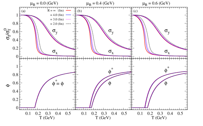
Figure 1: Temperature dependence of the (non)strange chiral condensates ($\sigma_{x}$) $\sigma_{y}$ panels (a, b and c) and the two Polyakov loops ($\phi$, $\phi^{*}$) panels (d, e and f) for several volume selections with $\mu_{B}$ = 0.0, 0.4 and 0.6 GeV.

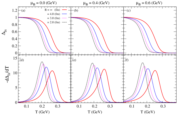
Figure 2: The same as in Fig.(1) but for the net-difference condensate ($\Delta_{ls}$) panels (a, b and c) and $d\Delta_{ls}/dT$ panels (d, e and f).

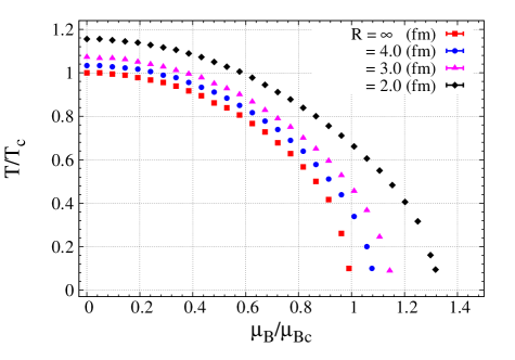
Figure 3: Chiral phase diagram for different volumes selections.

Figure. 1 shows the thermal dependence of the non-strange and strange chiral condensates ($\sigma_{x}$, $\sigma_{y}$) panels (a, b and c) and the Polyakov loops ($\phi$ and $\phi^{*}$) panels (d, e and f) for different volume selections and different $\mu_{B}$ values. The upper panels show that both $\sigma_{x}$ and $\sigma_{y}$ increase as the system volume is decreased, with larger sensitivity for the non-strange chiral condensates ($\sigma_{x}$). The lower panels show very little if any, volume dependence for $\phi$ and $\phi^{*}$ at different $\mu_{B}$.

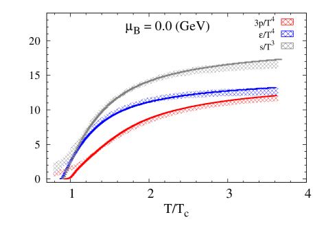
Figure 4: Comparison of the PQM model pressure density, energy density and entropy to results from LQCD. The comparisons are made for $\mu_{B}$ = 0.0 GeV; the lines indicate the PQM model calculations and the shaded areas indicate LQCD results from Ref. Borsanyi et al. (2014).

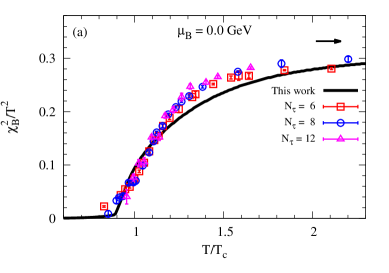
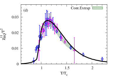
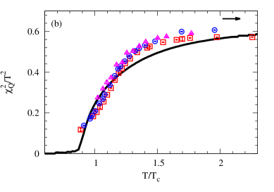
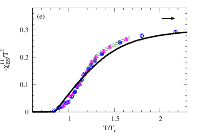
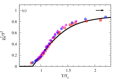
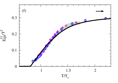
Figure 5: The thermal behavior of PQM model conserved charges fluctuation (a, b and c) and correlation (d, e and f) are compared with the same quantities obtained from the LQCD (symbols). The comparisons are made for $\mu_{B}=0$. The LQCD conserved charges fluctuation (a, b and c) and correlation (d, e and f) are taken from Ref Bazavov et al. (2012) tables (III, IV and V).

As pointed out PQM model contains strange and non-strange chiral condensates which reflect the chiral phase transitions. Using both chiral condensates we can investigate the finite volume effects on the $SU(3)$ $2+1$ PQM model chiral phase transition via the normalized net-difference condensate $\Delta_{ls}(T)$ as defined in Ref. Schaefer et al. (2010),

$$\Delta_{ls}(T) = \dfrac{\sigma_{x}-\dfrac{h_{x}}{h_{y}}\sigma_{y}}{\sigma_{x0}-\dfrac{h_{x}}{h_{y}}\sigma_{y0}},$$ (15)

where $h_{x}$ ($h_{y}$) are non-strange (strange) explicit symmetry breaking parameters.

Figure. 2 shows the thermal dependence of the normalized net-difference condensate $\Delta_{ls}$ panels (a, b and c) and $d\Delta_{ls}/dT$ panels (d, e and f) for different volume selections and different $\mu_{B}$ values. The upper panels indicate an increase in $\Delta_{ls}(T)$ as the system volume is decreased. The lower panels show that for fixed values of $R$ and $\mu_{B}$, the $d\Delta_{ls}/dT$ is peaking up at a specific point indicating the phase transition. The peak position is shifted toward lower temperature as the $\mu_{B}$ value increase.

The study of the phase diagram of the PQM model for at fixed volume could be done through mapping out the $\mu_{B}$ dependence of $\Delta_{q,s}(T)$. For a fixed $R$ and $\mu_{B}$ values, $d\Delta_{ls}/dT$ will peak up at a particular point expressing the phase transition. Therefore, the phase diagram can be studied by outlining such points for a wide range of baryon chemical potentials. Fig. 3 illustrates the effects of finite volume on the phase diagram. The parameters $T_{c}$ and $\mu_{Bc}$ represent the transition temperature at $\mu_{B}$ = 0.0 GeV and the transition chemical potential at low temperature respectively at $R$ = $\infty$. Our calculations reveal that the PQM model phase diagram in the $(\mu_{B},T)$-plane, increases with decreasing the system volume. For the $R$ = 2.0 (fm) the $\mu_{B}$ value at low temperature increased by about $30\%$ and the $T$ value at $\mu_{B}$ = 0.0 GeV increased by about $19\%$ from them values at $R$ = $\infty$ (fm).

III.2 Fluctuations and correlations of conserved charges

The thermodynamics quantities and (diagonal) off-diagonal susceptibilities can be determined by using the thermodynamic pressure as Bazavov et al. (2012),

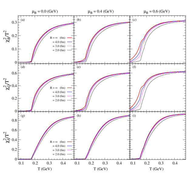
Figure 6: The thermal behavior of the normalized diagonal susceptibilities, $\chi^{2}_{BB}$, $\chi^{2}_{QQ}$ and $\chi^{2}_{SS}$, for several volume selections at $\mu_{B}$ = 0.0, 0.4 and 0.6 GeV.

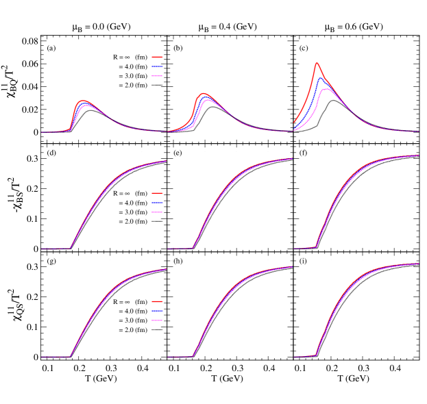
Figure 7: The thermal behavior of the normalized off-diagonal susceptibilities, $\chi^{11}_{BQ}$, $\chi^{11}_{BS}$ and $\chi^{11}_{QS}$, for several volume selections at $\mu_{B}$ = 0.0, 0.4 and 0.6 GeV.

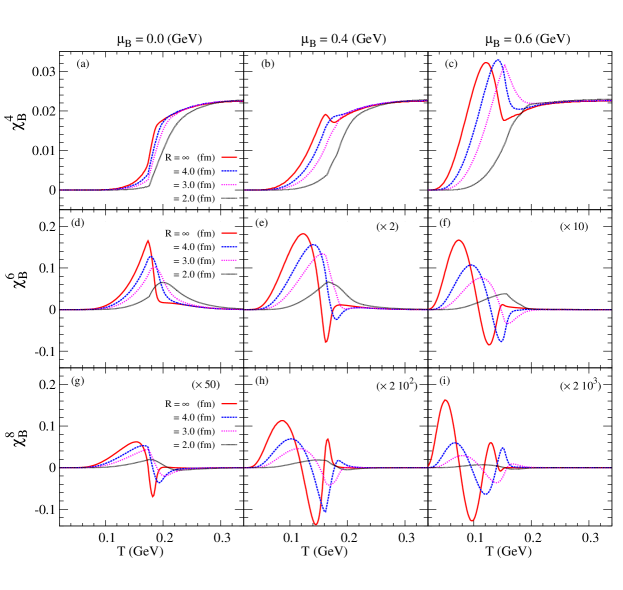
Figure 8: The thermal behavior of the higher order susceptibilities, $\chi^{4}_{B}$, $\chi^{6}_{B}$ and $\chi^{8}_{B}$, for several volume selections at $\mu_{B}$ = 0.0, 0.4 and 0.6 GeV.

$$p = -\Omega(T,\mu_{f}),$$ (16)

$$s = dp/dT,$$ (17)

$$\epsilon = Ts-p,$$ (18)

$$\chi^{ijk}_{BQS} = \frac{\partial^{i+j+k}(p)}{\partial(\mu_{B})^{i}\partial(\mu_{Q})^{j}\partial(\mu_{S})^{k}}.$$ (20)

where superscripts $i$, $j$ and $k$ run over integers that represent the derivatives orders. The indexes $B$, $Q$ and $S$ represent the conserved-quantities, baryon, charge, and strangeness, respectively. Eq. (20) illustrates the dependence of the (fluctuations) correlations of conserved charges on the temperature, chemical potential, and system volume. The susceptibilities evaluated first by computing the thermodynamic potential at vanishing $\mu_{f}$ and then expand the scaled thermodynamic potential in a Taylor series around $\mu_{f}/T=0$.

Before addressing the system volume effect, it is informative to contrast the PQM model thermodynamics quantities and (diagonal) off-diagonal susceptibilities calculations for ($\mu_{B}=0$ and $R=\infty$), to similar results from LQCD calculations Bazavov et al. (2012); Borsanyi et al. (2014). Such comparisons are presented in Figs. (4,5); which indicate a good agreement between the PQM model and LQCD Bazavov et al. (2012); Borsanyi et al. (2014). These comparisons could be improved spatially at low temperature by including the vector mesons sector to the PQM model. The influence of the finite volume on the model thermodynamics quantities has been discussed in our previous study Magdy et al. (2017).

Figure 6 displays the temperature dependence of the normalized conserved-fluctuations, baryon ($\chi_{BB}$), charge ($\chi_{QQ}$) and strangeness ($\chi_{SS}$), respectively. The results presented for several volume selections at three $\mu_{B}$ values, $\mu_{B}=0.0,~{}0.4~{}and~{}0.6$ GeV. Our results indicate that the normalized fluctuations decrease with the volume which quickly trends towards the infinite volume value at high temperature. The non-strange susceptibilities ($\chi^{2}_{BB}$ and $\chi^{2}_{QQ}$) shows a higher sensitivity to the volume change more than the strange susceptibility ($\chi^{2}_{SS}$). This weak sensitivity to the volume change of the strange quantities could be driving from the large mass of the strange quark.

Figure 7 shows the temperature dependence of the off-diagonal susceptibilities, $\chi^{2}_{BQ}$, $\chi^{2}_{BS}$ and $\chi^{2}_{SQ}$ for several volume selections and different $\mu_{B}$ values. The net baryons show a high correlation to the net charge and less correlation to the net strange. Our results indicate that the normalized correlations decrease with the volume which quickly trends towards the infinite volume value at high temperature. Also, the non-strange correlation ($\chi_{BQ}$) show a higher sensitivity to the volume change.

Also, the temperature dependence of the higher order baryon susceptibilities $\chi^{n}_{B}$ ($n$ = 4, 6 and 8) for different volume selections at $\mu_{B}$ values, $\mu_{B}$ = 0.0, 0.4 and 0.6 GeV are shown in Figure 8. The $n^{th}$-order susceptibilities decrease with the volume selections, and for $n=6,8$ they start to peak around the transition temperature $T_{c}$. Also, we observed a stronger oscillation in all higher harmonics as we increase the $\mu_{B}$ values.

IV Conclusions

In this work, we have used the $2+1$ $SU(3)$ Polyakov Quark-Meson model (PQM) framework to study the properties of the QCD medium produced at finite volume in heavy ion collisions. This model framework provides several conserved-quantities, baryon, charge, and strangeness which compare well with those obtained in LQCD calculations for vanishing $\mu_{B}$. Our calculations indicate that the conserved-quantities ($\chi^{ijk}_{BQS}$) are significantly influenced by finite volume effects. The calculated conserved-quantities decrease with the volume which quickly trends towards the infinite volume value at high temperature. Also, the non-strange quantities show a higher sensitivity to the volume change more than the strange once. Finally, PQM model conserved-quantities, suggests that the quark-hadron phase boundary is shifted to higher values of $\mu_{B}$ and $T$ with decreasing system volume.

References

- Fachini (2006) P. Fachini, “Experimental highlights of the RHIC program,” Proceedings, 10th Mexican Workshop on Particles and Fields (MWPF 2005), Part A and B: Morelia, Mexico, November 6-12, 2005, AIP Conf. Proc. 857, 62–75 (2006), arXiv:hep-ex/0605102 [hep-ex] .
- Monteno (2007) M. Monteno (ALICE), “The physics programme of the ALICE experiment at the LHC,” Perspectives in hadronic physics. Proceedings, 5th International Conference on perspectives in hadronic physics, particle-nucleus and nucleus-nucleus scattering at relativistic energies, Trieste, Italy, May 22-26, 2006, Nucl. Phys. A782, 283–290 (2007).
- Aoki et al. (2006) Y. Aoki, G. Endrodi, Z. Fodor, S. D. Katz, and K. K. Szabo, “The Order of the quantum chromodynamics transition predicted by the standard model of particle physics,” Nature 443, 675–678 (2006), arXiv:hep-lat/0611014 [hep-lat] .
- Ejiri (2008) Shinji Ejiri, “Canonical partition function and finite density phase transition in lattice QCD,” Phys. Rev. D78, 074507 (2008), arXiv:0804.3227 [hep-lat] .
- Pisarski and Wilczek (1984) Robert D. Pisarski and Frank Wilczek, “Remarks on the Chiral Phase Transition in Chromodynamics,” Phys. Rev. D29, 338–341 (1984).
- Lee (1972) Benjamin W Lee, “Chiral dynamics,” New York, NY : Gordon and Breach, B591, 129 p. (1972).
- Kovacs and Szep (2007) P. Kovacs and Zs. Szep, “The critical surface of the chiral quark model at non-zero baryon density,” Phys. Rev. D75, 025015 (2007), arXiv:hep-ph/0611208 [hep-ph] .
- Kovacs and Szep (2008) P. Kovacs and Zs. Szep, “Influence of the isospin and hypercharge chemical potentials on the location of the CEP in the mu(B) - T phase diagram of the chiral quark model,” Phys. Rev. D77, 065016 (2008), arXiv:0710.1563 [hep-ph] .
- Nambu and Jona-Lasinio (1961) Yoichiro Nambu and G. Jona-Lasinio, “Dynamical Model of Elementary Particles Based on an Analogy with Superconductivity. 1.” Phys. Rev. 122, 345–358 (1961), [,127(1961)].
- Fukushima (2004) Kenji Fukushima, “Chiral effective model with the Polyakov loop,” Phys. Lett. B591, 277–284 (2004), arXiv:hep-ph/0310121 [hep-ph] .
- Kahara and Tuominen (2008) Topi Kahara and Kimmo Tuominen, “Degrees of freedom and the phase transitions of two flavor QCD,” Phys. Rev. D78, 034015 (2008), arXiv:0803.2598 [hep-ph] .
- Wambach et al. (2010) Jochen Wambach, Bernd-Jochen Schaefer, and Mathias Wagner, “QCD Thermodynamics: Confronting the Polyakov-Quark-Meson Model with Lattice QCD,” Three days of strong interactions. Proceedings, EMMI Workshop and 26th Max Born Symposium, Wroclaw, Poland, July 9-11, 2009, Acta Phys. Polon. Supp. 3, 691–700 (2010), arXiv:0911.0296 [hep-ph] .
- Schaefer and Wagner (2009a) Bernd-Jochen Schaefer and Mathias Wagner, “On the QCD phase structure from effective models,” Heavy-ion collisions from the Coulomb barrier to the quark-gluon plasma. Proceedings, International Workshop on Nuclear Physics, 30th Course, Erice, Italy, September 16-24, 2008, Prog. Part. Nucl. Phys. 62, 381 (2009a), arXiv:0812.2855 [hep-ph] .
- Mao et al. (2010) Hong Mao, Jinshuang Jin, and Mei Huang, “Phase diagram and thermodynamics of the Polyakov linear sigma model with three quark flavors,” J. Phys. G37, 035001 (2010), arXiv:0906.1324 [hep-ph] .
- Fisher and Barber (1972) Michael E. Fisher and Michael N. Barber, “Scaling Theory for Finite-Size Effects in the Critical Region,” Phys. Rev. Lett. 28, 1516–1519 (1972).
- Abreu et al. (2006) L. M. Abreu, M. Gomes, and A. J. da Silva, “Finite-size effects on the phase structure of the Nambu-Jona-Lasinio model,” Phys. Lett. B642, 551–562 (2006), arXiv:hep-th/0610111 [hep-th] .
- Palhares et al. (2011) L. F. Palhares, E. S. Fraga, and T. Kodama, “Chiral transition in a finite system and possible use of finite size scaling in relativistic heavy ion collisions,” J. Phys. G38, 085101 (2011), arXiv:0904.4830 [nucl-th] .
- Fraga et al. (2011) Eduardo S. Fraga, Leticia F. Palhares, and Paul Sorensen, “Finite-size scaling as a tool in the search for the QCD critical point in heavy ion data,” Phys. Rev. C84, 011903 (2011), arXiv:1104.3755 [hep-ph] .
- Bhattacharyya et al. (2013) Abhijit Bhattacharyya, Paramita Deb, Sanjay K. Ghosh, Rajarshi Ray, and Subrata Sur, “Thermodynamic Properties of Strongly Interacting Matter in Finite Volume using Polyakov-Nambu-Jona-Lasinio Model,” Phys. Rev. D87, 054009 (2013), arXiv:1212.5893 [hep-ph] .
- Bhattacharyya et al. (2015a) Abhijit Bhattacharyya, Rajarshi Ray, and Subrata Sur, “Fluctuation of strongly interacting matter in the Polyakov–Nambu–Jona-Lasinio model in a finite volume,” Phys. Rev. D91, 051501 (2015a), arXiv:1412.8316 [hep-ph] .
- Magdy et al. (2017) Niseem Magdy, M. Csanád, and Roy A. Lacey, “Influence of finite volume and magnetic field effects on the QCD phase diagram,” J. Phys. G44, 025101 (2017), arXiv:1510.04380 [nucl-th] .
- Almasi et al. (2017) Gabor Almasi, Robert Pisarski, and Vladimir Skokov, “Volume dependence of baryon number cumulants and their ratios,” Phys. Rev. D95, 056015 (2017), arXiv:1612.04416 [hep-ph] .
- Borsanyi et al. (2014) Szabocls Borsanyi, Zoltan Fodor, Christian Hoelbling, Sandor D. Katz, Stefan Krieg, and Kalman K. Szabo, “Full result for the QCD equation of state with 2+1 flavors,” Phys. Lett. B730, 99–104 (2014), arXiv:1309.5258 [hep-lat] .
- Bazavov et al. (2012) A. Bazavov et al. (HotQCD), “Fluctuations and Correlations of net baryon number, electric charge, and strangeness: A comparison of lattice QCD results with the hadron resonance gas model,” Phys. Rev. D86, 034509 (2012), arXiv:1203.0784 [hep-lat] .
- Lenaghan et al. (2000) Jonathan T. Lenaghan, Dirk H. Rischke, and Jurgen Schaffner-Bielich, “Chiral symmetry restoration at nonzero temperature in the SU(3)(r) x SU(3)(l) linear sigma model,” Phys. Rev. D62, 085008 (2000), arXiv:nucl-th/0004006 [nucl-th] .
- Schaefer and Wagner (2009b) Bernd-Jochen Schaefer and Mathias Wagner, “The Three-flavor chiral phase structure in hot and dense QCD matter,” Phys. Rev. D79, 014018 (2009b), arXiv:0808.1491 [hep-ph] .
- Polyakov (1978) Alexander M. Polyakov, “Thermal Properties of Gauge Fields and Quark Liberation,” Phys. Lett. 72B, 477–480 (1978).
- Susskind (1979) Leonard Susskind, “Lattice Models of Quark Confinement at High Temperature,” Phys. Rev. D20, 2610–2618 (1979).
- Ratti et al. (2006) Claudia Ratti, Michael A. Thaler, and Wolfram Weise, “Phases of QCD: Lattice thermodynamics and a field theoretical model,” Phys. Rev. D73, 014019 (2006), arXiv:hep-ph/0506234 [hep-ph] .
- Ghosh et al. (2008) Sanjay K. Ghosh, Tamal K. Mukherjee, Munshi Golam Mustafa, and Rajarshi Ray, “PNJL model with a Van der Monde term,” Phys. Rev. D77, 094024 (2008), arXiv:0710.2790 [hep-ph] .
- Haas et al. (2013) Lisa M. Haas, Rainer Stiele, Jens Braun, Jan M. Pawlowski, and Jürgen Schaffner-Bielich, “Improved Polyakov-loop potential for effective models from functional calculations,” Phys. Rev. D87, 076004 (2013), arXiv:1302.1993 [hep-ph] .
- Schaefer et al. (2009) Bernd-Jochen Schaefer, Mathias Wagner, and Jochen Wambach, “QCD thermodynamics with effective models,” Proceedings, 5th International Workshop on Critical point and onset of deconfinement (CPOD 2009): Upton, USA, June 8-12, 2009, PoS CPOD2009, 017 (2009), arXiv:0909.0289 [hep-ph] .
- Tawfik et al. (2014) A. Tawfik, N. Magdy, and A. Diab, “Polyakov linear SU(3) model: Features of higher-order moments in a dense and thermal hadronic medium,” Phys. Rev. C89, 055210 (2014), arXiv:1405.0577 [hep-ph] .
- Kovács and Wolf (2015) Péter Kovács and György Wolf, “Chiral phase transition scenarios from the vector meson extended Polyakov quark meson model,” Proceedings, International Meeting of Excited QCD 2015: Tatranska Lomnica, Slovakia, March 8-14, 2015, Acta Phys. Polon. Supp. 8, 335 (2015), arXiv:1507.02064 [hep-ph] .
- Kovács et al. (2016) Peter Kovács, Zsolt Szép, and György Wolf, “Existence of the critical endpoint in the vector meson extended linear sigma model,” Phys. Rev. D93, 114014 (2016), arXiv:1601.05291 [hep-ph] .
- Fu (2013) Wei-jie Fu, “Fluctuations and correlations of hot QCD matter in an external magnetic field,” Phys. Rev. D88, 014009 (2013), arXiv:1306.5804 [hep-ph] .
- Bhattacharyya et al. (2015b) Abhijit Bhattacharyya, Rajarshi Ray, Subhasis Samanta, and Subrata Sur, “Thermodynamics and fluctuations of conserved charges in a hadron resonance gas model in a finite volume,” Phys. Rev. C91, 041901 (2015b), arXiv:1502.00889 [hep-ph] .
- Schaefer et al. (2010) Bernd-Jochen Schaefer, Mathias Wagner, and Jochen Wambach, “Thermodynamics of (2+1)-flavor QCD: Confronting Models with Lattice Studies,” Phys. Rev. D81, 074013 (2010), arXiv:0910.5628 [hep-ph] .