Prediction of Progression to Alzheimer’s disease with Deep InfoMax

Abstract

Arguably, unsupervised learning plays a crucial role in the majority of algorithms for processing brain imaging. A recently introduced unsupervised approach Deep InfoMax (DIM) is a promising tool for exploring brain structure in a flexible non-linear way. In this paper, we investigate the use of variants of DIM in a setting of progression to Alzheimer’s disease in comparison with supervised AlexNet and ResNet inspired convolutional neural networks. As a benchmark, we use a classification task between four groups: patients with stable, and progressive mild cognitive impairment (MCI), with Alzheimer’s disease, and healthy controls. Our dataset is comprised of 828 subjects from the Alzheimer’s Disease Neuroimaging Initiative (ADNI) database. Our experiments highlight encouraging evidence of the high potential utility of DIM in future neuroimaging studies.

I Introduction

According to [1], the economic costs of mental disorders have the highest impact on economic growth, direct and indirect costs and the statistical value of life. One essential tool for better understanding mental illness is to use noninvasive neuroimaging (e.g., structural magnetic resonance imaging (MRI) images) along with machine learning to learn brain structure.

Deep Learning has been integral to the successes of machine learning for numerous demanding real-world applications, e.g., state-of-the-art image classification [2] and self-driving cars [3]. While many of Deep Learning’s successes involve supervised learning, supervised approaches can fail when data annotation (e.g., labels) is limited or unavailable. When there is sufficient data, supervised models can not only perform well on holdout sets but provide representations that generalize well to other supervised settings [4]. However, when there is insufficient data, a supervised learner tends to discriminate on low-level (e.g., pixel-level, trivial) information, which hurts generalization performance. A model that generalizes well needs to extract meaningful high-level information (e.g., a collection of important features at the input level). In order to address this, many successful applications of machine learning to neuroscience rely on unsupervised learning [5, 6, 7, 8] to extract representations of brain imaging data. These representations are then used as input to an off-the-shelf classifier (i.e., semi-supervised learning).

However, prior work on unsupervised learning of brain imaging data is either linear or weakly nonlinear [5, 6] or are highly restrictive in parameterization [7], and do not represent flexible methodology for learning representations.

In this work, we explore using DIM [9] to learn deep non-linear representations of neuroimaging data as an output of a convolutional neural network. DIM works by maximizing the mutual information between a high-level feature vector and low-level feature maps of a highly flexible convolutional encoder network by training a second neural network that maximizes a lower bound on a divergence (probabilistic measure of difference) between the joint or the product of marginals of the encoder input and output. The estimates provided by this second network can be used to maximize the mutual information of the features in the encoder with the input. Unlike other popular unsupervised auto-encoding approaches such as VAE [10], DIM doesn’t require a decoder. Hence it significantly reduces memory requirements of the model for volumetric data.

We evaluate DIM by performing a downstream classification task between four groups: patients with stable and progressive MCI, with Alzheimer’s disease and healthy controls, using only the resulting representation from DIM as input to the classifier. We compare DIM to two convolutional networks with AlexNet [11] and ResNet [12] inspired architectures trained with supervised learning. On strict evaluation, we show comparable performance to supervised methods and to previously reported [13, 14, 15, 16] classification performance.

II Materials and Methods

II-A Deep InfoMax

Let $\mathbf{X}:=\{x^{(i)}\in\mathcal{X}\}$ and $\mathbf{Z}:=\{z^{(i)}\in\mathcal{Z}\}$ be the input and output variables of a neural network encoder, $E_{\phi}:\mathcal{X}\rightarrow\mathcal{Z}$ with parameters $\phi$, where $\mathcal{X}$, and $\mathcal{Z}$ are its domain and range. We wish to find the parameters that maximize the following objective:

$$(\hat{\phi},\hat{\theta})_{G}=\operatorname*{\arg\max}_{\phi,\theta}\hat{\mathcal{I}}_{\theta}(X;Z),$$ (1)

where $\hat{\mathcal{I}}_{\theta}$ is the mutual information estimate provided by a different network with parameters $\theta$, and $Z=E_{\phi}(X)$ is the output of the encoder.

A parametric estimator for the mutual information can be found by training a statistics network to maximize a lower bound based on the Fenchel-dual [17] or the Donsker-Varadhan representation [18, 19] of the Kullback–Leibler divergence $D_{KL}$. The Donsker-Varadhan-based estimator is a consistent, asymptotically unbiased estimator has been shown to outperform nonparametric estimators, and can also be used to improve deep generative models [19]. However, $D_{KL}$ is unbounded, which can be problematic if the above estimators are used for training deterministic neural network encoders. [9] showed that using an estimator based on the Jensen-Shannon divergence (JSD) (i.e., simple binary cross-entropy) is more stable and works well in practice, and it has been shown that this estimator also yields a good estimator for mutual information [9, 20]:

$$\begin{split}\hat{\mathcal{I}}_{\phi,\theta}^{\text{(JSD)}}(X;E_{\phi}(X)):=&\mathbb{E}_{\mathbb{P}_{X}}[-\text{sp}(-T_{\theta}(X,E_{\phi}(X)))]-\\ &\mathbb{E}_{\mathbb{P}_{X}\otimes\mathbb{P}_{X}}[\text{sp}(T_{\theta}(X^{\prime},E_{\phi}(X)))],\end{split}$$ (2)

where $T_{\theta}$ is a statistics network with parameters $\theta$, $\text{sp}=\log(1+e^{z})$ (softplus function) and $X^{\prime}$ is another input sampled from the data distribution independently from $X$. In addition, the Noise-Contrastive variant of the estimator (NCE) [21] was shown to work well in practice [9]:

$$\begin{split}&\hat{\mathcal{I}}_{\phi,\theta}^{\text{(NCE)}}(X;E_{\phi}(X)):=\\ &\mathbb{E}_{\mathbb{P}}\left[T_{\theta}(X,E_{\phi}(X))-\log\sum_{X^{\prime}\in\mathcal{X}_{b}}e^{T_{\theta}(X^{\prime},E_{\phi}(X))}\right].\end{split}$$ (3)

Here, $\mathcal{X}_{b}=\{X\}\bigcup\mathcal{X}_{n}$ are a set of samples where $\mathcal{X}_{n}$ are a set of negative samples drawn from the data distribution, such that there is exactly one positive example in $\mathcal{X}_{b}$ ($X$ occurs exactly once).

[9] showed that maximizing the mutual information between the complete input and output of an encoder are insufficient for learning good representations for downstream classification tasks, as this approach can still focus on lower-level “trivial” localized details. Instead, they show that maximizing the mutual information between the high-level representation, $Z=E_{\phi}(X)$ and patches of an input image can achieve highly competitive results. The intuition is that this approach encourages the high-level representation to learn information that is shared across the input. It is suitable for many classification tasks, as we expect that class-discriminative features should be evident across many spatial locations of the input. For a convolutional encoder $E$, the local DIM objective can be written in a compact form:

$$(\hat{\phi},\hat{\theta})_{L}=\operatorname*{\arg\max}_{\phi,\theta}\frac{1}{M^{2}}\sum_{i=1}^{M^{2}}\hat{\mathcal{I}}_{\phi,\theta}(C^{(i)}_{\phi}(X);E_{\phi}(X)),$$ (4)

where $C^{(i)}_{\phi}(X)$ is a feature map location from encoder (with a limited receptive field corresponding to an input patch with size $M$) at some intermediate layer of the network.

Due to stronger performance of AlexNet architecture (Section (II-B)) in our experiments (see Section (IV)) we used it as an encoder for DIM method. Last linear layer of AlexNet we changed with a layer for $64$-dimensional output representation.

To estimate mutual information using eq. (4) we used the encode-and-dot-product architecture (Fig. $6$ from [9]). First, patches $C^{(i)}_{\phi}(X)$ taken from third convolutional layer of AlexNet were mapped using convolutional encoder-and-dot architecture (Tab. $9$ from [9]) with $512$ units and their representation $Z=E_{\phi}(X)$ — linear encoder-and-dot architecture (Tab. $8$ from [9]). Then flattened encoded mappings of patches and representations were combined using the dot product to create real and fake samples efficiently. The real sample is a dot product of a “local” patch and its “global” representation mappings, while fake — between mapping of some “local” patch with global representation coming from an unrelated input. Eventually we estimated JSD based loss eq. (2) and NCE — eq. (3) using these samples. Since NCE needs to have more negative samples to be competitive with JSD [9], all possible combinations between the patch and representation mappings were used a similar way to create negative samples.

To evaluate the performance of the learned representation by DIM, we trained three additional neural networks using as input features output from last convolutional layer with size $128\times 2\times 2\times 2$, the first fully connected layer with $1024$ units, and final fully connected layer with $64$-dimensional representation, which we call as Conv, FC, and $Z$. The classifiers are composed of one fully-connected layer with $200$ hidden units, dropout [22] with $p=0.1$, batch normalization [23] and a ReLU [24] activation.

TABLE I: AlexNet and ResNet architectures

AlexNet
3D Conv $(1,64,5,2,0)$ - BN 3D - ReLU - MP 3D $(3,3)$
3D Conv $(64,128,3,1,0)$ - BN 3D - ReLU - MP 3D $(3,3)$
3D Conv $(128,192,3,1,1)$ - BN 3D - ReLU
3D Conv $(192,192,3,1,1)$ - BN 3D - ReLU
3D Conv $(192,128,3,1,1)$ - BN 3D - ReLU - MP 3D $(3,3)$
Linear $(1024,1024)$ - BN 1D - ReLU
Linear $(1024,4)$ - SoftMax - ArgMax
ResNet
3D Conv $(1,64,3,2,0)$ - BN 3D - ReLU - MP 3D $(3,3)$
Residual Layer 1
BB0 - 2 x (3D Conv $(64,64,3,1,1)$ - BN 3D - ReLU)
BB1 - 2 x (3D Conv $(64,64,3,1,1)$ - BN 3D - ReLU)
Residual Layer 2
BB0 - 3D Conv $(64,128,3,2,1)$ - BN 3D - ReLU
BB0 - 3D Conv $(128,128,3,1,1)$ - BN 3D - ReLU
BB0 downsample - 3D Conv $(64,128,3,2,1)$ - BN 3D
BB1 - 2 x (3D Conv $(128,128,3,2,1)$ - BN 3D - ReLU)
Residual Layer 3
BB0 - 3D Conv $(128,256,3,2,1)$ - BN 3D - ReLU
BB0 - 3D Conv $(256,256,3,1,1)$ - BN 3D - ReLU
BB0 downsample - 3D Conv $(128,256,3,2,1)$ - BN 3D
BB1 - 2 x (3D Conv $(256,256,3,2,1)$ - BN 3D - ReLU)
MaxPool 3D $(3,3)$
Linear $(2048,1024)$ - BN 1D - ReLU
Linear $(1024,4)$ - SoftMax - ArgMax

II-B Supervised baselines

As baselines we have considered supervised methods — two convolutional networks, one based on a simplified AlexNet [11] architecture and the other a ResNet [12] architecture. Both networks use convolutions and max pooling with volumetric kernels, batch normalization, ReLU and two fully connected layers in the end (see Tab. (I) for details). The notations in Tab. (I) denotes: BN for batch normalization, BB — a basic block, MP $(k,s)$ — max pooling with kernel size $k$ and stride $s$, for convolutions $(i,o,k,s,p)$ — a number of input and output channels, a kernel size, a stride and a padding respectively). Cross-entropy loss used as a training objective.

II-C Regularization

For small datasets, it is common to penalize the number of the model parameters by driving most of them to zero using $L_{1}$ regularization. Formally, this penalty is defined as:

$$L_{1}(\omega)=\lambda||\omega||_{1}=\lambda\sum_{i}|\omega_{i}|,$$ (5)

where $\omega$ is parameter vector of the model and $\lambda$ — coefficient. $L_{1}$ regularization imposes a sparse solution. This penalty is added to JSD, NCE and cross-entropy losses in different setting. For our experiments we used $\lambda=1$.

III Experiments

III-A Datasets and preprocessing

For the downstream classification task, the data was obtained from the ADNI database adni.loni.usc.edu (for up-to-date information, see www.adni-info.org). We use T1w MRI images of $830$ subjects with four different groups: patients with stable, and progressive MCI, Alzheimer’s disease and healthy controls.

Structural MRI (sMRI) data was pre-processed to grey matter volume (modulated) maps using SPM12 toolbox. To segment grey matter, the MRI images were spatially normalized and smoothed by 6 mm full width at half maximum (FWHM) 3D Gaussian kernel. After quality control, two subjects from ADNI dataset were excluded. The final dataset consisted of $828$ subjects with a volume size of $[121,145,121]$.

III-B Experimental setup

III-B1 Data

The dataset was divided in approximately $93\%$ and $7\%$ subjects for cross-validation and hold-out test sets using a stratified split. Then, $93\%$ subjects were split into five stratified folds.

For AlexNet and ResNet architectures, we used simple data augmentation of the training dataset to reduce overfitting to the small number of annotated samples available. Our augmentation consisted of zero padding and random cropping to size $128$ along all dimensions along with randomly flipping the input with probability $0.5$ for each axis. The whole brain was included in the crop.

For DIM, we didn’t use data augmentation, but we used zero padding to make sure that input size is equal to $128$ along all dimensions.

III-B2 Training

The models were trained using the AMSGrad [25] optimizer with learning rate $0.001$ for CNN models and $0.0001$ for DIM using a batch size of $8$ but dropping the incomplete last batch. The training of the supervised architectures was performed for $500$ epochs, DIM — for $1000$ epochs as pre-training and for $1000$ epochs for training the classifiers on top of frozen features from the encoder.

III-B3 Evaluation

Since the dataset is not completely balanced, the evaluation was performed using balanced accuracy [26], defined as the average of recall of each class (implementation in scikit-learn [27]).

III-B4 Implementation and hardware

The implementation was written using Deep Learning frameworks PyTorch [28] and Cortex [29]. The DIM code is based on openly available DIM implementation [30]. The experiments were performed on NVIDIA GeForce Titan X Pascal and 1080 Ti and 8 CPU threads.

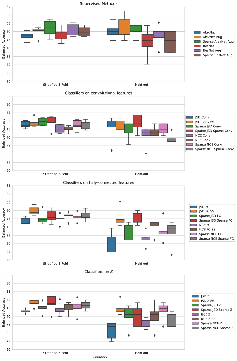
Figure 1: Performance of the models

TABLE II: Performance

Model Balanced Accuracy Stratified 5-Fold Balanced Accuracy Hold-out Mean gap Wilcoxon test Stat $p$-value AlexNet $47.31\pm 2.69$ $50.36\pm 4.62$ $3.05$ 6.5 $0.290$ AlexNet Aug $49.82\pm 3.18$ $52.14\pm 7.41$ $2.32$ 7.0 $0.554$ Sparse AlexNet Aug $51.85\pm 5.14$ $51.07\pm 3.91$ $0.78$ N/A N/A ResNet $47.9\pm 4.28$ $43.57\pm 8.71$ $4.33$ 10.0 0.034 ResNet Aug $50.72\pm 3.8$ $47.14\pm 6.51$ $3.58$ 14.0 0.039 Sparse ResNet Aug $50.07\pm 3.09$ $43.93\pm 6.26$ $6.14$ 10.0 0.033 JSD Conv $47.82\pm 2.11$ $45.36\pm 7.74$ $2.46$ 13.5 $0.052$ JSD Conv SS $48.83\pm 2.79$ $47.5\pm 3.24$ $1.33$ 13.5 $0.052$ Sparse JSD Conv $49.61\pm 2.35$ $44.29\pm 5.27$ $5.32$ 15.0 0.022 Sparse JSD Sparse Conv $49.29\pm 4.22$ $48.57\pm 5.27$ $0.72$ 6.0 $0.054$ NCE Conv $45.82\pm 2.82$ $40.71\pm 5.98$ $5.11$ 15.0 0.022 NCE Conv SS $45.08\pm 1.94$ $43.57\pm 2.99$ $1.51$ 10.0 0.034 Sparse NCE Conv $47.59\pm 3.21$ $45.0\pm 3.19$ $2.59$ 15.0 0.022 Sparse NCE Sparse Conv $47.23\pm 2.69$ $39.64\pm 2.93$ $7.59$ 15.0 0.022 JSD FC $44.18\pm 2.05$ $30.71\pm 6.11$ $13.47$ 15.0 0.022 JSD FC SS $49.77\pm 2.73$ $45.36\pm 5.73$ $4.41$ 14.0 0.040 Sparse JSD FC $45.42\pm 4.03$ $37.5\pm 5.05$ $7.92$ 15.0 0.022 Sparse JSD Sparse FC $46.6\pm 3.92$ $45.0\pm 3.87$ $1.6$ 15.0 0.022 NCE FC $44.89\pm 2.93$ $32.86\pm 4.48$ $12.03$ 15.0 0.022 NCE FC SS $46.53\pm 2.59$ $40.36\pm 4.66$ $6.17$ 15.0 0.020 Sparse NCE FC $46.2\pm 2.64$ $37.86\pm 6.49$ $8.34$ 15.0 0.022 Sparse NCE Sparse FC $47.01\pm 3.12$ $36.43\pm 7.84$ $10.58$ 15.0 0.022 JSD Z $43.12\pm 1.1$ $31.43\pm 5.14$ $11.69$ 15.0 0.021 JSD Z SS $48.44\pm 2.79$ $44.64\pm 4.19$ $3.8$ 15.0 0.022 Sparse JSD Sparse Z $47.74\pm 5.12$ $40.36\pm 6.39$ $7.38$ 15.0 0.022 Sparse JSD Z $45.27\pm 3.38$ $40.0\pm 6.98$ $5.27$ 15.0 0.022 NCE Z $44.14\pm 3.84$ $36.07\pm 2.93$ $8.07$ 15.0 0.022 NCE Z SS $45.28\pm 3.55$ $40.0\pm 7.84$ $5.28$ 14.0 0.040 Sparse NCE Sparse Z $46.63\pm 2.69$ $37.14\pm 4.45$ $9.49$ 15.0 0.022 Sparse NCE Z $45.27\pm 4.85$ $43.21\pm 5.56$ $2.06$ 15.0 0.021

IV Results

The final trained models used further to evaluate the performance were selected based on the best-balanced accuracy but from a checkpoint where the validation score was lower than the training score. We gave the model a burn-in period before applying this rule to deal with initial stochasticity. The models notations are as follows: Aug denotes augmentation of the training dataset, the first sparse — a model trained with $L_{1}$ regularization, the second — a classifier on top of the frozen features from encoders trained using $L_{1}$ regularization, SS — stands for training an unsupervised model with an additional supervised loss from $Z$-classifier.

Table II reports the balanced accuracy rates including mean, standard deviation values, and the gap between mean values on cross-validation and hold-out. The bold text distinguishes the best scores and the name of the models. The last column shows $p$-value and statistic for the one-sided Wilcoxon test. The bold $p$-values indicate acceptance of the null hypothesis. The test was performed to compare each method with the best model (Sparse AlexNet Aug) based on the five values of balanced accuracy on hold-out. An alternative hypothesis is that the model Sparse AlexNet Aug is better. Fig. 1 highlights the distributions of the performance.

With all modifications, ResNet shows a lower performance on hold-out (at most $47.14\pm 6.51$) than AlexNet. It is reasonable since the capacity of the ResNet architecture is larger and the dataset is small. For $\alpha=0.05$ Wilcoxon test also rejects H0 supporting the worse performance of ResNet. Performance of JSD Conv, JSD Conv SS, Sparse JSD Sparse Conv, AlexNet, AlexNet Aug is statistically indistinguishable from that of Sparse AlexNet Aug. Follows that unsupervised DIM has comparable performance to supervised methods.

Among DIM variants, JSD has higher scores than NCE. Lower scores of NCE can be explained by its requirement of a large number of negative samples during training to be competitive with JSD. Our dataset is not large enough to support the needed level of negative sampling.

The best score with convolutional features—$48.57\pm 5.27$—was obtained by an encoder and classifier trained with $L_{1}$ regularization which is the Sparse JSD Sparse Conv model. For features from the fully-connected layer — JSD FC SS model with $45.36\pm 5.73$ using semi-supervised loss was the best. However, Sparse JSD Sparse FC has similar results $45.0\pm 3.87$ and a smaller mean gap $1.6$ but it has a lower mean cross-validation score by $3.17\%$ . For the smallest $64$-dimensional representation, semi-supervised model JSD Z SS gives the best performance $44.64\pm 4.19$, but similar result $43.21\pm 5.56$ were obtained by Sparse NCE Z model. Semi-supervised loss and $L_{1}$ regularization improved models’ generalization by reducing the gap between cross-validation and hold-out scores. The observed degradation in performance between Conv, FC, and $Z$ can be explained by the reduced capacity of the features. $L_{1}$ regularization and dropout could also be adjusted. However, a more compact input representation can be of independent use, for example, for dimensionality reduction.

In previous studies, the best reported accuracy for the ResNet architecture in a 4-class sMRI classification task was $54\%$ [13], while stacked autoencoders (SAE) [15] reached for sMRI only $46.30\pm 4.24$ and for sMRI+PET $53.79\pm 4.76$, and DW-S²MTL [16] — for sMRI $47.83$ or for sMRI+PET+CSF $53.72$. Our values can’t be completely comparable since the evaluation is different. Reproduced ResNet can be used as a proxy to estimate performance relative to this prior work. Note, however, it is not one of the best-performing methods in our study.

V Conclusions

This work proposes an unsupervised method DIM for learning representations from structural neuroimaging data. The evaluation of the prediction of progression to Alzheimer’s disease demonstrates results comparable to supervised methods. In the future, we will scale up our experiments with increased sample size and address the cases of other diseases. Our future efforts will also be focused on the multi-modal fusion of brain imaging data [31] to increase the predictive strength of the model.

References

- [1] S. Trautmann, J. Rehm, and H.-U. Wittchen, “The economic costs of mental disorders: Do our societies react appropriately to the burden of mental disorders?” EMBO reports, p. e201642951, 2016.
- [2] G. Huang, Z. Liu, L. Van Der Maaten, and K. Q. Weinberger, “Densely connected convolutional networks,” in 2017 IEEE Conference on Computer Vision and Pattern Recognition (CVPR). IEEE, 2017, pp. 2261–2269.
- [3] Y. Xiong, R. Liao, H. Zhao, R. Hu, M. Bai, E. Yumer, and R. Urtasun, “Upsnet: A unified panoptic segmentation network,” arXiv preprint arXiv:1901.03784, 2019.
- [4] L. Zhang, T. Xiang, and S. Gong, “Learning a deep embedding model for zero-shot learning,” in 2017 IEEE Conference on Computer Vision and Pattern Recognition (CVPR). IEEE, 2017, pp. 3010–3019.
- [5] V. D. Calhoun, T. Adali, G. D. Pearlson, and J. Pekar, “A method for making group inferences from functional mri data using independent component analysis,” Human brain mapping, vol. 14, no. 3, pp. 140–151, 2001.
- [6] R. D. Hjelm, V. D. Calhoun, R. Salakhutdinov, E. A. Allen, T. Adali, and S. M. Plis, “Restricted boltzmann machines for neuroimaging: an application in identifying intrinsic networks,” NeuroImage, vol. 96, pp. 245–260, 2014.
- [7] E. Castro, R. D. Hjelm, S. M. Plis, L. Dinh, J. A. Turner, and V. D. Calhoun, “Deep independence network analysis of structural brain imaging: application to schizophrenia,” IEEE transactions on medical imaging, vol. 35, no. 7, pp. 1729–1740, 2016.
- [8] S. M. Plis, D. R. Hjelm, R. Salakhutdinov, E. A. Allen, H. J. Bockholt, J. D. Long, H. J. Johnson, J. S. Paulsen, J. A. Turner, and V. D. Calhoun, “Deep learning for neuroimaging: a validation study,” Frontiers in neuroscience, vol. 8, p. 229, 2014.
- [9] R. D. Hjelm, A. Fedorov, S. Lavoie-Marchildon, K. Grewal, A. Trischler, and Y. Bengio, “Learning deep representations by mutual information estimation and maximization,” arXiv preprint arXiv:1808.06670, 2018.
- [10] D. P. Kingma and M. Welling, “Auto-encoding variational bayes,” arXiv preprint arXiv:1312.6114, 2013.
- [11] A. Krizhevsky, I. Sutskever, and G. E. Hinton, “Imagenet classification with deep convolutional neural networks,” in Advances in Neural Information Processing Systems 25, F. Pereira, C. J. C. Burges, L. Bottou, and K. Q. Weinberger, Eds. Curran Associates, Inc., 2012, pp. 1097–1105.
- [12] K. He, X. Zhang, S. Ren, and J. Sun, “Deep residual learning for image recognition,” in Proceedings of the IEEE conference on computer vision and pattern recognition, 2016, pp. 770–778.
- [13] A. Abrol, M. Bhattarai, A. Fedorov, Y. Du, S. Plis, and V. Calhoun, “Deep residual learning for neuroimaging: An application to predict progression to alzheimer’s disease,” bioRxiv, p. 470252, 2018.
- [14] S. Vieira, W. H. Pinaya, and A. Mechelli, “Using deep learning to investigate the neuroimaging correlates of psychiatric and neurological disorders: Methods and applications,” Neuroscience & Biobehavioral Reviews, vol. 74, pp. 58–75, 2017.
- [15] S. Liu, S. Liu, W. Cai, H. Che, S. Pujol, R. Kikinis, D. Feng, M. J. Fulham, and ADNI, “Multimodal neuroimaging feature learning for multiclass diagnosis of alzheimer’s disease,” IEEE Transactions on Biomedical Engineering, vol. 62, no. 4, pp. 1132–1140, April 2015.
- [16] H.-I. Suk, S.-W. Lee, D. Shen, A. D. N. Initiative et al., “Deep sparse multi-task learning for feature selection in alzheimer’s disease diagnosis,” Brain Structure and Function, vol. 221, no. 5, pp. 2569–2587, 2016.
- [17] S. Nowozin, B. Cseke, and R. Tomioka, “f-gan: Training generative neural samplers using variational divergence minimization,” in Advances in Neural Information Processing Systems, 2016, pp. 271–279.
- [18] M. D. Donsker and S. S. Varadhan, “Asymptotic evaluation of certain markov process expectations for large time. iv,” Communications on Pure and Applied Mathematics, vol. 36, no. 2, pp. 183–212, 1983.
- [19] M. I. Belghazi, A. Baratin, S. Rajeswar, S. Ozair, Y. Bengio, A. Courville, and R. D. Hjelm, “Mine: mutual information neural estimation,” arXiv preprint arXiv:1801.04062, 2018.
- [20] B. Poole, S. Ozair, A. van den Oord, A. A. Alemi, and G. Tucker, “On variational lower bounds of mutual information.”
- [21] A. v. d. Oord, Y. Li, and O. Vinyals, “Representation learning with contrastive predictive coding,” arXiv preprint arXiv:1807.03748, 2018.
- [22] N. Srivastava, G. Hinton, A. Krizhevsky, I. Sutskever, and R. Salakhutdinov, “Dropout: a simple way to prevent neural networks from overfitting,” The Journal of Machine Learning Research, vol. 15, no. 1, pp. 1929–1958, 2014.
- [23] S. Ioffe and C. Szegedy, “Batch normalization: Accelerating deep network training by reducing internal covariate shift,” arXiv preprint arXiv:1502.03167, 2015.
- [24] V. Nair and G. E. Hinton, “Rectified linear units improve restricted boltzmann machines,” in Proceedings of the 27th international conference on machine learning (ICML-10), 2010, pp. 807–814.
- [25] S. J. Reddi, S. Kale, and S. Kumar, “On the convergence of adam and beyond,” arXiv preprint arXiv:1904.09237, 2019.
- [26] K. H. Brodersen, C. S. Ong, K. E. Stephan, and J. M. Buhmann, “The balanced accuracy and its posterior distribution,” in Pattern recognition (ICPR), 2010 20th international conference on. IEEE, 2010, pp. 3121–3124.
- [27] F. Pedregosa, G. Varoquaux, A. Gramfort, V. Michel, B. Thirion, O. Grisel, M. Blondel, P. Prettenhofer, R. Weiss, V. Dubourg, J. Vanderplas, A. Passos, D. Cournapeau, M. Brucher, M. Perrot, and E. Duchesnay, “Scikit-learn: Machine learning in Python,” Journal of Machine Learning Research, vol. 12, pp. 2825–2830, 2011.
- [28] A. Paszke, S. Gross, S. Chintala, G. Chanan, E. Yang, Z. DeVito, Z. Lin, A. Desmaison, L. Antiga, and A. Lerer, “Automatic differentiation in pytorch,” 2017.
- [29] rdevon/cortex: A machine learning library for pytorch. [Online]. Available: https://github.com/rdevon/cortex
- [30] rdevon/dim: Deep infomax (dim), or ”learning deep representations by mutual information estimation and maximization”. [Online]. Available: https://github.com/rdevon/DIM
- [31] V. D. Calhoun and J. Sui, “Multimodal fusion of brain imaging data: a key to finding the missing link (s) in complex mental illness,” Biological psychiatry: cognitive neuroscience and neuroimaging, vol. 1, no. 3, pp. 230–244, 2016.