A new approach to the LSZ reduction formula

Abstract

Lehmann, Symanzik and Zimmermann (LSZ) proved a theorem showing how to obtain the S-matrix from time-ordered Green functions. Their result, the reduction formula, is fundamental to practical calculations of scattering processes. A known problem is that the operators that they use to create asymptotic states create much else besides the intended particles for a scattering process. In the infinite-time limits appropriate to scattering, the extra contributions only disappear in matrix elements with normalizable states, rather than in the created states themselves, i.e., the infinite-time limits of the LSZ creation operators are weak limits. The extra particles that are created are in a different region of space-time than the intended scattering process. To be able to work with particle creation at non-asymptotic times, e.g., to give a transparent and fully deductive treatment for scattering with long-lived unstable particles, it is necessary to have operators for which the infinite-time limits are strong limits. In this paper, I give an improved method of constructing such operators. I use them to give an improved systematic account of scattering theory in relativistic quantum field theories, including a new proof of the reduction formula. Among the features of the new treatment are explicit Feynman rules for the vertices corresponding to the creation operators, both for the LSZ ones and for the new ones. With these I make explicit calculations to illustrate the problems with the LSZ operators and their solution with the new operators. Not only do these verify the existence of the extra particles created by the LSZ operators and indicate a physical interpretation, but they also show that the extra components are so large that their contribution to the norm of the state is ultra-violet divergent in renormalizable theories. Finally, I discuss the relation of this work to the work of Haag and Ruelle on scattering theory.

I Introduction

The reduction formula of Lehmann, Symanzik and Zimmermann [1] (LSZ) is very important for applications of quantum field theory (QFT) to experiment because it shows how to compute S-matrix elements from time-ordered Green functions, including the correct external line factors.

Unfortunately, there are some problems, as was realized a long time ago — see the papers by Haag [4, 5], Ruelle [6], and Hepp [7]. The problems do not in fact impact the validity of the reduction formula itself, or even the validity of LSZ’s proof. Instead, the problems manifest themselves when one tries extending the LSZ methods to more general situations. As we will see, such cases occur quite dramatically when the operators used by LSZ to create asymptotic particles are applied in experimentally relevant situations at finite times instead of infinite times.

More explicitly, suppose we are given a single-particle positive-energy wave function $f(x)$. Then LSZ define a time-dependent operator $a^{\dagger}_{f}(t)$ that is intended to create a single particle in the in-state or the out-state in the limit that $t\to-\infty$ or $t\to+\infty$, with the particle’s state corresponding to the wave function $f$. However, when one of these operators acts on the vacuum, what is created is a lot more than the intended particle; taking time to infinity does not help. This will be illustrated in Sec. IX.3 with the aid of explicit perturbative calculations. Moreover, we will see that, the extra contributions are not merely nonzero, but in a renormalizable QFT are also generically ultra-violet (UV) divergent, as measured by the norm of the state that is created.

In the restricted context of the matrix elements used to obtain the S-matrix, a careful application of the infinite-time limits, as in the LSZ paper, does remove the extra contributions. This can be characterized [4, 6] by saying that the limits used by LSZ are weak limits, but not strong limits. (See App. A for characterization of these concepts, together with summaries of methods by which it can be determined which kind of limit is applicable in particular cases.)

In contrast, for an operator $A^{\dagger}_{f}(t,\Delta t)$ that actually does asymptotically create a single particle only, then the strong limit exists. As indicated by the notation, it will be useful to introduce an extra parameter $\Delta t$ that is a range of time involved in defining the operator; its inverse is essentially an uncertainty in energy. The operator creates a single particle in the limit $\Delta t\to\infty$. Its application to creating particles in a scattering process involves taking both $t$ and $\Delta t$ to infinity in such a way that $\Delta t/|t|\to 0$.

Such an operator allows one to make an adequate treatment when the strict limits of infinite time are not taken. Such would be the case for treating long-lived but unstable particles or for a fully deductive treatment of neutrino scattering and oscillations. The extra particles created by using the original LSZ operator instead of the new operator would be detected in a suitably located detector.

Textbook treatments given for these situations typically start from the strict infinite-time formalism for standard scattering. They then graft on something like a semiclassical analysis of isolated free particles, with a good dose of intuition and hand-waving.

The primary purpose of the paper is to provide an improved proof that overcomes the problems just described.

In the LSZ paper, the creation operator $a^{\dagger}_{f}(t)$ involves just an integral over all space, with the field (and its time derivative) being taken at one specific value of time $t$. It is the use of integrals at fixed time that causes the problems, essentially by a kind of application of an uncertainty principle: A fixed time implies infinite uncertainty in energy.

The main innovation applied in the present paper is to find a good way of defining the operator $A^{\dagger}_{f}(t,\Delta t)$, by averaging $a^{\dagger}_{f}(t)$ over a range of time. Many conceptual subtleties then robustly disappear.

Related techniques were used by Haag and Ruelle in their formulation of scattering theory [4, 6]. But their method was formulated somewhat differently, and in a way that calculations using their operators difficult. They focused heavily on mathematical aspects of the theory as opposed to possible applications. The different construction given in the present paper makes its much easier to treat the asymptotics and allows a simplification of the proof of the reduction formula. The new construction provides simple explicit formulas for the new operators both in coordinate space and momentum space. See Sec. XIV for a comparison of the new method with the Haag-Ruelle method.

It is important to emphasize that, as regards the LSZ reduction formula itself, the issues just summarized concern its proof. In the case that we use a theory in which all particles are massive and that we treat only scattering of exactly stable particles, the LSZ reduction formula remains correct and unchanged.

One advantage of the new formulation is that once the new definition of $A^{\dagger}_{f}(t,\Delta t)$ has been provided, then the derivation of the S-matrix is essentially a straightforward calculation. The bulk of this paper primarily concerns motivation, examples, and derivations of the prerequisites for performing the calculations. As already mentioned, another advantage of the new methods are that they allow straightforward extensions to situations at non-asymptotic times, e.g., to treat unstable particles. Boyanovsky [12] has recently treated the space-time properties of the decay of unstable particles, and encountered complications that are closely related to the issues treated here. In particular, he provides an independent calculation of the ultra-violet divergence in the state created by an LSZ operator.

Another possible extension is to scattering with massless particles. As is well-known, the postulates of standard scattering theory fail in theories with massless particles. A fully systematic treatment requires extensions or modifications to the versions of scattering theory that are valid for massive particles. There is recent interest, e.g., [13, 14], in finding better treatments for the massless case. Off-shell or finite-time Green functions do exist in such theories. Therefore what is in question is the nature of the infinite-time limits and their relation to physically implementable scattering. A strategy for defining good finite-time approximations to the creation of single particles could be very useful to finding a better formulation of the infinite-time limits with massless particles. The formalism presented in this paper is suitable for use in perturbative calculational examples that can be used to test the formulation of general abstract theorems.

II Overall view: starting point, motivations, strategy

II.1 Aims

A primary technical aim is the determination of the S-matrix in a quantum field theory (QFT) from its Green functions.. A related aim is to construct definitions of operators that can be applied to the vacuum state to construct in and out states, which are states of well-separated individual particles. The operators give a construction of the state space of the theory in terms of field operators applied to the vacuum, with parameterizations of the states that are suitable for experimentally relevant scattering processes.

We assume that a QFT exists, as specified by its set of fields and its Lagrangian density, that it obeys the standard properties of QFTs, and that the task is to compute S-matrix elements from the Green functions. In doing so, one also verifies many of the properties of scattering processes that underlie the definition and use of the S-matrix. Motivations for the emphasis on Green functions will be given next.

II.2 Position with respect to logical framework for QFT

Underlying those practical aims is a deeper issue. This concerns what it means to solve a particular QFT, and what exactly is the logic by which the results are derived and checked.

A QFT is specified by listing a set of basic fields, which are operator valued functions of space-time (strictly speaking, operator-valued distributions), and by postulating certain of their properties, notably equal-time canonical commutation relations (ETCCRs) and equations of motion. Normally these are determined from a formula for a Lagrangian density in terms of the basic fields. A solution entails determining what the state space is and how the operators act on it, after which one can compute quantities of experimental interest. Of course, after solving for the state space and the operators by deductions from the initial postulates that specify the theory, it is useful to verify self-consistency by showing that the constructed operators do obey the postulated properties.

In contrast, the situation is rather different in the case of the non-relativistic quantum mechanics of a finite number of particles. In the first formulation of quantum mechanics, i.e., Heisenberg’s matrix mechanics, the above procedure was followed to determine the matrices that implement the position and momentum operators. See the paper by Born and Jordan [16] for the case of the harmonic oscillator. In normal current terminology, we would say that the matrices consist of the matrix elements of the corresponding operators between energy eigenstates.

It was quickly realized, at least in effect, that in these relatively simple theories there is a unique representation of the ETCCRs, up to unitary equivalence. Thus the state space and how the operators act on it are determined uniquely. States can then be realized as Schrödinger wave functions. That is all independent of the details of the Hamiltonian, e.g., as to what the potential is. Predictions of the theory can be determined by solving the Schrödinger equation for time dependence of the state or for energy eigenstates, etc.

In QFT, the situation is radically different. Because of the infinite number of degrees of freedom, there is no longer a unique representation of the ETCCRs. Moreover, it is found that the different representations get used. Calculations show pathologies and inconsistencies — e.g., [17, 18] — if one assumes that the state space of an interacting theory is the same as that of a free theory and that the operators at one fixed time are the same in both theories, as is done to define the interaction picture. Moreover, Haag’s theorem [19, 20, 2] guarantees that this is not just a difficulty in particular examples, but a general property of relativistic QFTs.

One way of stating this is that the Hilbert space of states for an interacting theory is orthogonal to that for a corresponding free theory. However, the Hilbert spaces for the free and interacting theories are isomorphic, so one could alternatively arrange things such that the Hilbert spaces are the same; but in that case, Haag’s theorem shows that the free and interacting fields cannot be related by a unitary transformation, contrary to what happens in the widely used interaction picture.

These results considerably complicate the derivation of useful consequences from a given QFT. Solving the theory requires, implicitly or explicitly, a determination of the state space and the action of the field operators on it. The vast majority of work on making predictions effectively evades the issue of what the states and operators are. Perturbative calculations using Feynman graphs give only matrix elements. Non-perturbative calculations using Monte-Carlo lattice methods provide an implementation of the functional integral of a QFT, and have as their immediate target time-ordered Green functions continued to Euclidean time; thus they give vacuum-expectation values of certain operators.

Nevertheless, underlying any derivation of the methods from the foundational postulates of a QFT is an assumption that there are operators acting on the state space.

A useful way of handling the issues is to make the Green functions then primary target of calculations, such as in Refs. [21, 22, 10, 11]. In perturbation theory, the Green functions can be obtained from the Gell-Mann-Low formula. This allows the calculation of Green functions in the full theory from certain matrix elements in the free theory. The formula can be derived from the functional integral, but it is often also derived from a use of the interaction picture. Normally Haag’s theorem prevents the consistent use of the interaction picture. But in deriving the Gell-Mann-Low formula, the derivation using the interaction picture can be first applied to a regulated theory with a finite number of degrees of freedom. A projection onto the exact ground state can be made with the use of the evolution operator at a time that is somewhat rotated towards imaginary values [23]. Then the regulators can be removed to give a continuum theory in an infinite volume of space, with the application of any necessary renormalization. In a correct derivation, the numerator and denominator of the Gell-Mann-Low formula both contain a factor $|\langle 0|0;{\rm free}\rangle|^{2}$, the squared overlap of the vacuum states in the interacting and free theories. Haag’s theorem manifests itself in this overlap going to zero when the infinite volume limit is taken. But since the factor cancels between numerator and denominator, the final results for the Green function are valid and well-behaved in the limit that the regulators are removed. Even though the operators and states have rather singular properties as the regulator is removed, the Green functions have smooth limits.

The Green functions obey equations of motion that encode both the equations of motion for the fields and their (anti)commutation relations on a “surface of quantization”. Since it is readily proved that the perturbative expansion of Green functions obeys these equations, we know that at least the perturbative solution for Green functions exists independently of any qualms one might have about the adequacy of particular textbook derivations from first principles, e.g., concerning the existence of the functional-integral representation of Minkowski-space Green functions, or the asymptotic limits used in applying the interaction picture.

An approach via Green functions recognizes that the particle content and scattering processes arise as emergent phenomena from the solution of a QFT. The particle concept in interacting relativistic QFTs is essentially identical to the quasi-particle concept [24, Sec. 5.7] in condensed matter physics, certainly if one uses the word “particle” to refer not only to strictly stable particles but also to unstable and confined particles. The primary practical differences in condensed matter physics are that there is an obvious preferred rest frame, and that the background medium is at non-zero temperature, thereby giving rise to notable dissipative effects.

Then the project initiated by LSZ of obtaining the S-matrix (and in fact other matrix elements of time-ordered operators) is in effect a determination of the state space of the theory in a useful basis and of how the field operators are implemented in that basis. (In fact, there are two useful sets of basis states, one for incoming states in a scattering process and one for outgoing states.)

Hence the overall logic is to start with the postulates specifying a particular QFT. From them one deduces methods for calculating Green functions, with care taken to avoid invalidation of the derivations by Haag’s theory. Finally one constructs the scattering states, and the other consequences of the theory from the Green functions. The LSZ reduction formula is the core tool to get from the off-shell Green functions to S-matrix elements and to matrix elements of any operator.

In contrast to the Green function route, many books — e.g., [25] — take the S-matrix as primary. Such an approach can be useful, e.g., [10, 11], to gain initial insight from low-order perturbation theory about elementary experimental implications of a given QFT. But in a complete treatment, use of the S-matrix as primary is problematic. In its most natural form, such a treatment assumes that the spectra of the free and interacting theories are the same (e.g., p. 110 of [25]) and hence that the particle types are in one-to-one correspondence with the fields. But such an assumption is generally very incorrect. For example, in the Standard Model, the only elementary fields that correspond to particles in the strict sense of scattering theory are those for the photon, electron, and neutrinos. The particles, or quasiparticles, that correspond to the other fields are either unstable (e.g., muon), or confined (e.g., quarks), or both. On the other hand, there is a large collection of stable bound states (proton, and many nuclei, atoms and molecules) that do not correspond to the elementary fields.

Moreover, in theories with massless particles, the standard theory of scattering and the S-matrix needs modification, as manifested by the existence of infra-red divergences in calculations of the S-matrix and cross sections by standard methods. In contrast, the off-shell Green functions do not have such problems. So it is again useful to separate the issue of solving the theory, as manifested in the Green functions, from that of determining properties of scattering.

Furthermore, treatments that take the S-matrix as primary typically use the interaction picture in a way that runs badly afoul of Haag’s theorem. For example, the treatment in Ref. [25] starts from an assertion, (3.1.12) and (3.1.13), of the large-time asymptotics of interaction-picture states. The assertion is intended to capture in mathematical form the intuitive notion of states approaching states of separated particles. But Haag’s theorem ensures that the asserted asymptotic properties are simply wrong, and in a sense infinitely wrong. The incorrectness of the stated properties is readily verified by low order perturbative calculations, as was well-known in the early 1950s, e.g., [17, 18].

These direct derivations of the S-matrix can be regarded as constructing a perturbative solution of a theory on the basis of certain postulates about its properties. Once that solution has been constructed, it can be investigated whether the constructed solution self-consistently has the properties attributed to the solution. In this case, it is readily seen from perturbative calculations that the solution does not have these properties. A critical question is whether the final answer for the perturbative solution is correct despite the false hypotheses used to derive it or whether the answer itself is wrong. In this case it is only the hypotheses that are wrong, and the solution can be derived by better methods.

II.3 Structure of presentation

The overall structure of the presentation and derivation in this paper is summarized by the following items:

1. In Sec. IV a review is given of the formulation of scattering theory in terms of Fock-space structures for the in- and out-states. This is a framework that is strongly motivated by an examination of what happens in scattering processes and in non-relativistic quantum mechanics [3, 26]. From a logical point of view, it may be best to regard the formalism as a conjecture, to be a target of and then verified by subsequent derivations.

2. Then there is made an examination of the asymptotics of Green functions in coordinate space, for large positive and negative times, together with the relation to properties of the Green functions in momentum space, notably the poles in external lines. This motivates which properties of Green functions need to be examined to derive the S-matrix.

3. An essential part of the specification of in- and out-states concerns wave functions for the center-of-mass motion of each of the asymptotic particles. These are used in both momentum and coordinate space. The coordinate-space wave functions are simply positive energy solutions of the Klein-Gordon equation. In Sec. VII an account of properties of these wave functions is given, since these properties will be used in essential ways in the derivation of the reduction formula. The material is by no means new, but it is not always found in standard textbooks, so it is useful to provide a systematic exposition here.

4. In Sec. VIII, a statement of the reduction formula is given, an improved derivation of which is the aim of later sections.

5. In Sec. IX it is shown how to construct creation operators for particles in the in- and out-states, such that the necessary limits of infinite time are valid as strong limits, rather than merely weak limits. As a motivation for the definitions, the LSZ versions of the operators are stated, and their deficiencies are demonstrated with the aid of explicit perturbative calculations. The structure of the definition of the new creation operators will be such as to trivially avoid the problems, as we will see after the proof of the reduction formula.

   Some elementary properties of the operators are obtained in Sec. X.

6. In Sec. XI, the new derivation of the reduction formula is made. The derivation starts from the vacuum matrix elements of products the new annihilation and creation operators, and then analyzes the relevant limits of large times.

7. In Sec. XII, verification of important properties of the new annihilation and creation operators is made, including that the infinite-time limits are strong limits.

8. Finally, some indications of possible generalizations are summarized in Sec. XIII, and a comparison with the Haag-Ruelle method is given in Sec. XIV.

III Notations and conventions

All the fields are in the Heisenberg picture, so that the states are time-independent. If renormalization needs to be considered, then the fields are taken to be renormalized fields; for these, the time-ordered Green functions are finite. The space-time metric has the signature $\mathbin{+}\mathbin{-}\mathbin{-}\mathbin{-}$.

In expanding quantities like fields in integrals over modes, I use the Lorentz invariant form of integral with the same convention and notation as Itzykson and Zuber’s book [27]. Thus a free Klein-Gordon field obeys

$$\phi_{{\rm free}}(t,\boldsymbol{x})=\int\frac{\mathop{{\mathrm{d}}^{3}{}\boldsymbol{k}}\nolimits}{(2\pi)^{3}\,2E_{\boldsymbol{k}}}\times\\ \times\left[a_{\boldsymbol{k},{\rm free}}e^{-iE_{\boldsymbol{k}}t+i\boldsymbol{k}\cdot\boldsymbol{x}}+a_{\boldsymbol{k},{\rm free}}^{\dagger}e^{iE_{\boldsymbol{k}}t-i\boldsymbol{k}\cdot\boldsymbol{x}}\right],$$ (1)

where $E_{\boldsymbol{k}}=\sqrt{\boldsymbol{k}^{2}+m^{2}}$, $m$ is the mass of the particle, and the commutators of the annihilation and creation operators are

$$[a_{\boldsymbol{k},{\rm free}},a_{\boldsymbol{l},{\rm free}}^{\dagger}]=2E_{\boldsymbol{k}}\,(2\pi)^{3}\,\delta^{(3)}(\boldsymbol{k}-\boldsymbol{l}),$$ (2a)

$$[a_{\boldsymbol{k},{\rm free}},a_{\boldsymbol{l},{\rm free}}]=[a_{\boldsymbol{k},{\rm free}}^{\dagger},a_{\boldsymbol{l},{\rm free}}^{\dagger}]=0.$$ (2b)

Correspondingly, the normalization condition for single-particle momentum eigenstates $|\boldsymbol{k}\rangle=a_{\boldsymbol{k},{\rm free}}^{\dagger}|0\rangle$ is

$$\langle\boldsymbol{k}|\boldsymbol{l}\rangle=2E_{\boldsymbol{k}}\,(2\pi)^{3}\,\delta^{(3)}(\boldsymbol{k}-\boldsymbol{l}).$$ (3)

Following Itzykson and Zuber, I define a notation $\mathop{\widetilde{\mathop{{\mathrm{d}}{}k}\nolimits}}\nolimits$ by

$$\int\mathop{\widetilde{\mathop{{\mathrm{d}}{}k}\nolimits}}\nolimits\,\dots \stackrel{{\scriptstyle\textrm{def}}}{{=}}\int\frac{\mathop{{\mathrm{d}}^{3}{}\boldsymbol{k}}\nolimits}{2E_{\boldsymbol{k}}(2\pi)^{3}}\,\dots$$

$$=\int\frac{\mathop{{\mathrm{d}}^{4}{}k}\nolimits}{(2\pi)^{4}}\,2\pi\delta(k^{2}-m^{2})\,\theta(k^{0})\,\dots.$$ (4)

Then we can write

$$\phi_{{\rm free}}(x)=\int\mathop{\widetilde{\mathop{{\mathrm{d}}{}k}\nolimits}}\nolimits\left[a_{\boldsymbol{k},{\rm free}}e^{-{ik\cdot x}}+a_{\boldsymbol{k},{\rm free}}^{\dagger}e^{{ik\cdot x}}\right].$$ (5)

I use the standard convention that a 4-vector like $x$ is notated in italics, while its spatial part is in boldface: $\boldsymbol{x}$.

Note that many authors use different conventions for the momentum eigenstates and wave functions. Correspondingly they have slightly different integrals in their versions of Eqs. (1)–(5) and in later equations.

We will make much use of time-ordered Green functions of the quantum field(s) of a theory. When there is one scalar field, which is the only case we will treat explicitly, we use the notation

$$G_{N}(x_{1},\dots,x_{N})\stackrel{{\scriptstyle\textrm{def}}}{{=}}\langle 0|T\prod_{j=1}^{N}\phi(x_{j})|0\rangle.$$ (6)

Its Fourier transform is defined by

$$\tilde{G}_{N}(k_{1},\dots,k_{N})\stackrel{{\scriptstyle\textrm{def}}}{{=}}\int\mathop{{\mathrm{d}}^{4}{}x_{1}}\nolimits\dots\mathop{{\mathrm{d}}^{4}{}x_{N}}\nolimits\times\\ \times e^{-ik_{1}\cdot x_{1}\mathbin{-}\dots\mathbin{-}ik_{N}\cdot x_{N}}\,G_{N}(x_{1},\dots,x_{N}),$$ (7)

with the convention that the $k_{j}$ are treated as momenta flowing into the Green function.

IV Scattering formalism

In this section, I review the formalism of in- and out-states that is used to formulate scattering theory in QFT. Although the material is more or less standard, it is useful to present it here, so that the necessary background and motivation for the reduction formula are given. It is also useful to organize the presentation to show certain differences in relativistic QFT compared with the situation in non-relativistic quantum mechanics.

The essential point is to provide a quantum-mechanical formulation of the intuitive idea of scattering, to do this in Heisenberg picture, and to do it in such a way as to be immune to issues such as those associated with Haag’s theorem and the non-existence of the interaction picture in QFT. Later sections will be concerned with relating the results to properties of operators and Green functions. When we prove the reduction formula, we are, among other things, effectively verifying that the formalism is indeed appropriate.

We are familiar with scattering processes, where at asymptotically large negative times a system’s state consists of two incoming free particles each moving classically. The particles scatter in some essentially finite region of space and time, and then at asymptotically large positive times, the state is a linear combination of various states consisting of outgoing free particles propagating classically. Experimental apparatus makes a measurement of the final state, with approximate localization of the detected outgoing particles in both space-time and momentum. In normal applications of QFT we only examine the momenta of the incoming and outgoing particles, and present calculational results in terms of the S-matrix (commonly in perturbative approximations).

IV.1 Scattering in the Schrödinger formulation of non-relativistic quantum mechanics

We first examine how the intuitive ideas about scattering are translated into quantum-mechanical form for systems of a finite number of non-relativistic particles with interactions mediated by potentials. The results can be formalized in terms of Schrödinger wave functions. Essential simplifications compared with QFT are:

• Haag’s theorem does not apply, so that the state space and the action of operators on it can be specified independently of the interaction. Schrödinger wave functions are effectively an expansion of states in terms of eigenstates of the position operators. Thus for a single particle we can write its Schrödinger picture state as

  $$|\psi,t\rangle=\int\mathop{{\mathrm{d}}^{3}{}\boldsymbol{a}}\nolimits\,|\boldsymbol{a}\rangle\,\psi(\boldsymbol{a},t),$$ (8)

  where $|\boldsymbol{a}\rangle$ is an eigenstate of the position operators with eigenvalues $\boldsymbol{a}$, and with the normalization condition

  $$\langle\boldsymbol{a}|\boldsymbol{b}\rangle=\delta^{(3)}(\boldsymbol{a}-\boldsymbol{b}).$$ (9)

  Observe that the state $|\boldsymbol{a}\rangle$ can be considered as having the wave function $f_{\boldsymbol{a}}(\boldsymbol{x})=\delta^{(3)}(\boldsymbol{x}-\boldsymbol{a})$. This is a distribution but not an ordinary function of position. So any valid use has to be considered as having an implicit or explicit integral with a smooth test function, as in Eq. (8). Effectively, one can treat $|\boldsymbol{a}\rangle$ as a state-valued distribution, i.e., a mapping from smooth functions to states. (Similar conceptual issues will apply when we work with momentum eigenstates in QFT.)

• Asymptotically when particles are separated by much more than the range of the potential, their propagation is simply that of free particles: the action of the potential operator on the state goes to zero. In contrast, in an interacting QFT, one can never turn off the interactions inside a particle. Relative to a corresponding free theory, even a single particle in a QFT can be thought of as consisting of a complicated linear combination of states in the free field theory. Moreover, Haag’s theorem guarantees (in the relativistic case) that these linear combinations are badly divergent. So effectively the free and interacting theories use different state spaces, which are dynamically determined. Hence expressing the true single particle states in terms of free-particle states is a manner of speaking, only suggestive of the true situation.

The simplest case is of one particle in an external potential that falls off rapidly enough at large distance, and that has no bound states. The Hamiltonian is

$$H=\frac{\boldsymbol{\widehat{p}}^{2}}{2m}+V(\boldsymbol{\widehat{x}}).$$ (10)

Here, to avoid confusion between operators and numeric-valued variables of the same name, I have labeled QM operators with a hat.

Scattering is implemented by a wave function $\psi(\boldsymbol{x},t)$ that solves the time-dependent Schrödinger equation. As $t\to-\infty$, $\psi(\boldsymbol{x},t)$ approaches the wave function for a freely propagating particle:

$$\psi(\boldsymbol{x},t)\stackrel{{\scriptstyle t\to-\infty}}{{\to}}\int\frac{\mathop{{\mathrm{d}}^{3}{}p}\nolimits}{(2\pi)^{3}}\,\tilde{\psi}_{{\rm in}}(\boldsymbol{p})\,e^{-iE_{\boldsymbol{p}}t+i\boldsymbol{p}\cdot\boldsymbol{x}},$$ (11)

where $E_{\boldsymbol{p}}=\boldsymbol{p}^{2}/(2m)$ and $\tilde{\psi}_{{\rm in}}(\boldsymbol{p})$ is a momentum-space wave function narrowly peaked around some value of momentum. At large positive times, the state has a similar expansion, but with different coefficients:

$$\psi(\boldsymbol{x},t)\stackrel{{\scriptstyle t\to+\infty}}{{\to}}\int\frac{\mathop{{\mathrm{d}}^{3}{}\boldsymbol{p}}\nolimits}{(2\pi)^{3}}\,\tilde{\psi}_{{\rm out}}(\boldsymbol{p})\,e^{-iE_{\boldsymbol{p}}t+i\boldsymbol{p}\cdot\boldsymbol{x}}.$$ (12)

IV.2 Basis in- and out-states in elementary quantum mechanics

To obtain a formulation in Heisenberg picture, we use two sets of eigenfunctions of the Hamiltonian with certain boundary conditions at spatial infinity. These give what we will call the in- and out-basis functions.

For the wave functions $\phi_{\boldsymbol{p};\,{\rm in}}(\boldsymbol{x})$ for the in-basis we write

$$\phi_{\boldsymbol{p};\,{\rm in}}(\boldsymbol{x})=e^{i\boldsymbol{p}\cdot\boldsymbol{x}}+g_{\boldsymbol{p};\,{\rm in}}(\boldsymbol{x}),$$ (13)

with a corresponding state-vector notated as $|\boldsymbol{p};\,{\rm in}\rangle$. It is an eigenfunction of the Hamiltonian,

$$H|\boldsymbol{p};\,{\rm in}\rangle=E_{\boldsymbol{p}}|\boldsymbol{p};\,{\rm in}\rangle,$$ (14)

that obeys the boundary condition that at large $\boldsymbol{x}$, the scattered wave $g_{\boldsymbol{p};\,{\rm in}}(\boldsymbol{x})$ has only an outgoing part at large $|\boldsymbol{x}|$, i.e.,

$$g_{\boldsymbol{p};\,{\rm in}}(\boldsymbol{x})\stackrel{{\scriptstyle|\boldsymbol{x}|\to\infty}}{{\to}}\frac{e^{i|\boldsymbol{p}||\boldsymbol{x}|}}{|\boldsymbol{x}|}f_{\boldsymbol{p};\,{\rm in}}(\theta,\phi),$$ (15)

with no incoming term. That is, there is no term with $x$ dependence of the form $e^{-i|\boldsymbol{p}||\boldsymbol{x}|}/|\boldsymbol{x}|$. The factor $f_{\boldsymbol{p};\,{\rm in}}(\theta,\phi)$ is a function of the polar angle of $\boldsymbol{x}$; it is a result of the solution.

Thus at large $\boldsymbol{x}$, the function $\phi_{\boldsymbol{p};\,{\rm in}}(\boldsymbol{x})$ is a combination of a plane wave and an outgoing scattered wave:

$$\phi_{\boldsymbol{p};\,{\rm in}}(\boldsymbol{x})=e^{i\boldsymbol{p}\cdot\boldsymbol{x}}+\frac{e^{i|\boldsymbol{p}||\boldsymbol{x}|}}{|\boldsymbol{x}|}f_{\boldsymbol{p};\,{\rm in}}(\theta,\phi)+O(1/\boldsymbol{x}^{2}).$$ (16)

The out-basis functions are defined similarly, except that the scattered wave has only an incoming part:

$$\phi_{\boldsymbol{p};\,{\rm out}}(\boldsymbol{x})=e^{i\boldsymbol{p}\cdot\boldsymbol{x}}+\frac{e^{-i|\boldsymbol{p}||\boldsymbol{x}|}}{|\boldsymbol{x}|}f_{\boldsymbol{p};\,{\rm out}}(\theta,\phi)+O(1/\boldsymbol{x}^{2}).$$ (17)

The two solutions can be related by a time-reversal transformation.

Then a general solution of the time-dependent Schrödinger equation is of the form

$$\psi(\boldsymbol{x},t)=\int\frac{\mathop{{\mathrm{d}}^{3}{}\boldsymbol{p}}\nolimits}{(2\pi)^{3}}\,\tilde{\psi}_{{\rm in}}(\boldsymbol{p})\,e^{-iE_{\boldsymbol{p}}t}\,\phi_{\boldsymbol{p};\,{\rm in}}(\boldsymbol{x}),$$ (18)

i.e.,

$$|\psi;t\rangle=\int\frac{\mathop{{\mathrm{d}}^{3}{}\boldsymbol{p}}\nolimits}{(2\pi)^{3}}\,|\boldsymbol{p};\,{\rm in}\rangle\,\tilde{\psi}_{{\rm in}}(\boldsymbol{p})\,e^{-iE_{\boldsymbol{p}}t}.$$ (19)

A stationary-phase argument can be used to show that at large negative times, only the $e^{i\boldsymbol{p}\cdot\boldsymbol{x}}$ term in Eq. (16) contributes. The contribution of the scattered wave is strongly suppressed. Then the wave function $\psi(\boldsymbol{x},t)$ obeys the condition of a free incoming particle, as in Eq. (11). At large positive time, the scattered wave also contributes.

A reversed set of conditions applies to an expansion in the out-basis states.

The Heisenberg-picture state is defined to be the Schrödinger-picture state at time 0. Thus we can expand the Heisenberg state in terms of either set of basis states:

$$|\psi\rangle_{\rm H} =\int\frac{\mathop{{\mathrm{d}}^{3}{}\boldsymbol{p}}\nolimits}{(2\pi)^{3}}\,|\boldsymbol{p};\,{\rm in}\rangle\,\tilde{\psi}_{{\rm in}}(\boldsymbol{p})$$ (20a)

$$=\int\frac{\mathop{{\mathrm{d}}^{3}{}\boldsymbol{p}}\nolimits}{(2\pi)^{3}}\,|\boldsymbol{p};\,{\rm out}\rangle\,\tilde{\psi}_{{\rm out}}(\boldsymbol{p}).$$ (20b)

We now show that the inner product of the basis states of the same type has the standard normalization:

$$\langle\boldsymbol{p};\,{\rm in}|\boldsymbol{q};\,{\rm in}\rangle=(2\pi)^{3}\delta^{(3)}(\boldsymbol{p}-\boldsymbol{q})=\langle\boldsymbol{p};\,{\rm out}|\boldsymbol{q};\,{\rm out}\rangle.$$ (21)

(Since we are in a non-relativistic situation, we omit the $2E_{\boldsymbol{p}}$ factor that we use in the relativistic case.) The derivation is by considering the inner product $\langle\psi_{1};t|\psi_{2};t\rangle$ of two states of the form given in Eq. (18). Because time-evolution is unitary, the inner product is independent of $t$. From the expansion in the in-basis states we have

$$\langle\psi_{1};t|\psi_{2};t\rangle=\int\frac{\mathop{{\mathrm{d}}^{3}{}\boldsymbol{p}}\nolimits}{(2\pi)^{3}}\int\frac{\mathop{{\mathrm{d}}^{3}{}\boldsymbol{q}}\nolimits}{(2\pi)^{3}}\times\\ \times\tilde{\psi}_{1;\,{\rm in}}^{*}(\boldsymbol{p})\tilde{\psi}_{2;\,{\rm in}}(\boldsymbol{q})\,\langle\boldsymbol{p};\,{\rm in}|\boldsymbol{q};\,{\rm in}\rangle.$$ (22)

But because of the time-independence of the inner product, we can also compute in the limit of $t\to-\infty$, when we can replace the wave functions by plane waves, as at Eq. (11), and then we use the usual inner product of plane waves to give

$$\langle\psi_{1};-\infty|\psi_{2};-\infty\rangle=\int\frac{\mathop{{\mathrm{d}}^{3}{}\boldsymbol{p}}\nolimits}{(2\pi)^{3}}\,\tilde{\psi}_{1;\,{\rm in}}^{*}(\boldsymbol{p})\tilde{\psi}_{2;\,{\rm in}}(\boldsymbol{p}).$$ (23)

A similar derivation applies to the expansion in out-basis states. Hence the scattering solutions obey (21), and this normalization follows directly from the normalization of the plane-wave part in (13).

Observe that the inner product (21) has to be interpreted in a distributional sense, i.e., integrated with (smooth) test function(s). This is evidenced by the presence of a delta-function. Trying to calculate the inner product directly, by an integral over $\boldsymbol{x}$ of $\phi_{\boldsymbol{q};\,{\rm in}}(\boldsymbol{x})^{\phi}_{\boldsymbol{p};\,{\rm in}}(\boldsymbol{x})$ is prevented by the lack of convergence of the integral.

IV.3 The S-matrix in elementary quantum mechanics

The S-matrix can be defined as a relation between the expansions in the 2 sets of basis functions given in (20). Let us work in the Heisenberg picture. We have

$$|\psi\rangle_{\rm H} =\int\frac{\mathop{{\mathrm{d}}^{3}{}\boldsymbol{p}}\nolimits}{(2\pi)^{3}}\,|\boldsymbol{p};\,{\rm in}\rangle\,\tilde{\psi}_{{\rm in}}(\boldsymbol{p})$$

$$=\int\frac{\mathop{{\mathrm{d}}^{3}{}\boldsymbol{p}}\nolimits}{(2\pi)^{3}}\frac{\mathop{{\mathrm{d}}^{3}{}\boldsymbol{k}}\nolimits}{(2\pi)^{3}}\,|\boldsymbol{k};\,{\rm out}\rangle\,\langle\boldsymbol{k};\,{\rm out}|\boldsymbol{p};\,{\rm in}\rangle\,\tilde{\psi}_{{\rm in}}(\boldsymbol{p}).$$ (24)

Then the S-matrix could be defined by

$$S_{\boldsymbol{k},\boldsymbol{p}}=\langle\boldsymbol{k};\,{\rm out}|\boldsymbol{p};\,{\rm in}\rangle,=\int\mathop{{\mathrm{d}}^{3}{}\boldsymbol{x}}\nolimits\phi_{\boldsymbol{k};\,{\rm out}}^{*}(\boldsymbol{x})\phi_{\boldsymbol{p};\,{\rm in}}(\boldsymbol{x}).$$ (25)

Then the two sets of expansion coefficients are related by

$$\tilde{\psi}_{{\rm out}}(\boldsymbol{k})=\int\frac{\mathop{{\mathrm{d}}^{3}{}\boldsymbol{p}}\nolimits}{(2\pi)^{3}}\,S_{\boldsymbol{k},\boldsymbol{p}}\,\tilde{\psi}_{{\rm in}}(\boldsymbol{p}).$$ (26)

As with many other formulas involving basis states labeled by momenta, the definition (25) is to be interpreted distributionally, i.e., when integrated with smooth test functions. If nothing else the $\boldsymbol{x}$ integral in (25) would otherwise diverge. So we could better define the S-matrix by Eq. (26), as a relation between expansion coefficients; effectively this will be the definition we use in QFT, thereby avoiding a definition directly in terms of basis states.

In working with the S-matrix, it is convenient to extract all the delta functions, i.e., to make explicit the intrinsically distributional part, and thus to write

$$S_{\boldsymbol{k},\boldsymbol{p}}=(2\pi)^{3}\delta^{(3)}(\boldsymbol{k}-\boldsymbol{p})+2\pi\delta(E_{\boldsymbol{k}}-E_{\boldsymbol{p}})\,\mathcal{A}(\boldsymbol{k},\boldsymbol{p}).$$ (27)

The amplitude $\mathcal{A}(\boldsymbol{k},\boldsymbol{p})$ is an ordinary function of its arguments (but restricted to the case that the energies of the two momenta are equal). This amplitude is a natural target of Feynman-graph calculations, especially in the generalization of these results to QFT.

It can be shown that it is related to the function $f$ that is the coefficient of the $1/x$ term in (16) by

$$\mathcal{A}(\boldsymbol{k},\boldsymbol{p})=\frac{-2\pi i}{m}f_{\boldsymbol{p};\,{\rm in}}(\theta_{\boldsymbol{k}},\phi_{\boldsymbol{k}}).$$ (28)

A fundamental derivation from first principles can be made by computing the asymptotics of $\psi(\boldsymbol{x},t)$ for $t\to\pm\infty$; this is done starting from the expansion in $|\boldsymbol{p};\,{\rm in}\rangle$, using stationary phase methods, and then matching onto a plane-wave expansion as $t\to\infty$. That expansion has coefficients $\tilde{\psi}_{{\rm out}}(\boldsymbol{k})$. Somewhat shorter derivations can be made with the aid of insights as to what happens in the limit that the expansion function $\tilde{\psi}_{{\rm in}}(\boldsymbol{p})$ approaches a delta function, so that the $t\to-\infty$ wave function approaches a plane wave cut off at very large distances. An appropriate function would be

$$\tilde{\psi}_{{\rm in}}(\boldsymbol{p})=\left(\frac{4\pi}{\Delta p^{2}}\right)^{3/2}e^{-(\boldsymbol{p}-\boldsymbol{p}_{0})^{2}/\Delta p^{2}},$$ (29)

with $\Delta p\to 0$.

IV.4 Generalization

When we go to relativistic QFT, we will need the multiparticle case, where we will write basis states with arbitrarily many particles as

$$|\boldsymbol{p}_{1},\dots,\boldsymbol{p}_{n};\,{\rm in}\rangle,$$ (30a)

$$|\boldsymbol{q}_{1},\dots,\boldsymbol{q}_{n};\,{\rm out}\rangle,$$ (30b)

often with the natural generalizations to allow labels for particle type and for spin states. However, unlike the case of Schrödinger wave-function theory, we will not have a direct definition of these objects, e.g., as wave functions that are eigenfunctions of the Hamiltonian subject to certain boundary conditions. So we will formulate the necessary concepts in terms of normalizable states with specified asymptotic particle content, and arrange that further derivations use only normalizable states as starting points.

In a QFT we construct normalizable states by applying products of field operators to the vacuum and integrating with smooth functions of the positions of the field operators. The taking of linear combinations then gives general states. A main aim of this paper is to provide a construction of this kind for a state that has a specified momentum content for asymptotic incoming particles, and similarly for outgoing particles.

This implies that it is useful to formulate the methods in terms of normalizable states only, i.e., states genuinely in the Hilbert space of the theory, and only after that to provide a formulation involving the momentum-dependent basis states. That is done by the natural generalization of the construction given above (29). To implement the idea of states with specified incoming particle content, we will first specify the relevant properties of a Fock space decomposition of the state space. This simply matches the corresponding structures in wave-function theory. Later sections will provide constructions of states that implement the Fock space. The physical interpretation as free incoming particles of definite momentum content will be determined by the localization of the particles as determined by locations of the fields used to construct the states, and by a computation of the effect of applying the momentum operator on the states. In Sec. XI.2, we will find that indeed the particles propagate asymptotically along the appropriate classical trajectories and have the expected momenta.

The states for which we actually give a construction have product wave functions. This will be sufficient, because the taking of linear combinations gives general states in the Hilbert space, i.e., the states with product wave functions form a complete set in the sense used in Hilbert space.

After the construction of states with specified content in the initial or final states, various quantities of interest can be computed from the Green functions of the theory; these include S-matrix elements, and matrix elements of operators between specified states.

In Schrödinger wave-function theory, basis states for incoming particles, as in (30), are defined to be the sum of a multidimensional plane wave and what is asymptotically an out-going wave. Whenever a bound state is one of the asymptotic particles, then the proper generalization of the plane wave idea is that there is a plane wave factor for the center-of-mass coordinate of the bound state, and this is multiplied by the wave function depending on the relative coordinates of the elementary constituents.

We now abstract from the above discussion the Fock-space formalism that applies in QFT to states with specified asymptotic particle content. For this presentation following, we assume that there is one type of particle, and that it is a boson of nonzero mass $m$. Generalizations to multiple types of particle, including fermions, are elementary, and can be worked out from material in standard textbooks.

Given the basis in-states (30a), a general normalizable state is specified by an infinite array of momentum-space wave functions, $\underline{f}=(f_{0},f_{1},\ldots)$, and has the form

$$|\underline{f};\,{\rm in}\rangle=\sum_{n=0}^{\infty}\frac{1}{n!}\int\prod_{j=1}^{n}\mathop{\widetilde{\mathop{{\mathrm{d}}{}p_{j}}\nolimits}}\nolimits f_{n}(\boldsymbol{p}_{1},\ldots,\boldsymbol{p}_{n})\,|\boldsymbol{p}_{1},\dots,\boldsymbol{p}_{n};\,{\rm in}\rangle.$$ (31)

The wave functions are assumed to be symmetric in their arguments, and the $1/n!$ factor is a choice of normalization to reflect the multiple counting of identical states in the integral over all momenta. We have now restored the relativistic normalization for integrals. Note that the label “${\rm in}$” in $|\underline{f};{\rm in}\rangle$ does not refer to a particular type of state. Rather it refers to the specification of the state in terms of a given array of momentum-space functions $\underline{f}$, which specify the state in terms of its particle content at asymptotically large negative times. Equation (31) is an expansion of one particular Heisenberg-picture state, so the coefficients have no time dependence.

Exactly similar considerations apply to treating states with given momentum content in the asymptotic future, i.e., states denoted $|\underline{f};{\rm out}\rangle$.

The Hilbert-space structure can now be specified without mention of the basis states themselves, by referring everything to the normalizable states $|\underline{f};{\rm in}\rangle$. The inner product is then

$$\langle\underline{f};\,{\rm in}|\underline{g};\,{\rm in}\rangle\\ =\sum_{n=0}^{\infty}\frac{1}{n!}\int\left(\prod_{j=1}^{n}\mathop{\widetilde{\mathop{{\mathrm{d}}{}p_{j}}\nolimits}}\nolimits\right)g_{n}^{*}(\boldsymbol{p}_{1},\ldots,\boldsymbol{p}_{n})f_{n}(\boldsymbol{p}_{1},\ldots,\boldsymbol{p}_{n}).$$ (32)

IV.5 Product states

For our derivations of the S-matrix etc, it will be sufficient to restrict to product states. Thus given momentum-space wave functions $\tilde{f}_{1}(\boldsymbol{p})$ and $\tilde{f}_{2}(\boldsymbol{p})$ for single particles, we will define a two-particle state $|f_{1},f_{2};\,{\rm in}\rangle$ to have the wave function

$$\tilde{f}_{1}(\boldsymbol{p}_{1})\tilde{f}_{2}(\boldsymbol{p}_{2})+\tilde{f}_{2}(\boldsymbol{p}_{1})\tilde{f}_{1}(\boldsymbol{p}_{2}).$$ (33)

Since we will often work with related functions in coordinate space, I now use the over-tilde to denote momentum-space quantities.

More generally an $n$-particle initial state $|f_{1},\dots,f_{n};\,{\rm in}\rangle$ is defined to have the wave function

$$\prod_{j=1}^{n}\tilde{f}_{j}(\boldsymbol{p}_{j})+\mbox{permutations},$$ (34)

with a total of $n!$ terms. A product state $|g_{1},\dots,g_{n};\,{\rm out}\rangle$ with specified content in the far future is defined similarly.

In the notation using basis states, we write, for example, a two-particle initial product state as

$$|f_{1},f_{2};\,{\rm in}\rangle=\int\mathop{\widetilde{\mathop{{\mathrm{d}}{}p_{1}}\nolimits}}\nolimits\,\mathop{\widetilde{\mathop{{\mathrm{d}}{}p_{2}}\nolimits}}\nolimits\,|\boldsymbol{p}_{1},\boldsymbol{p}_{2};\,{\rm in}\rangle\,\tilde{f}_{1}(\boldsymbol{p}_{1})\tilde{f}_{2}(\boldsymbol{p}_{2}).$$ (35)

The symmetrization appropriate to bosons is enforced by the basis states, and no separate symmetrization of the wave function is needed.

With the conventions of Sec. III, the normalization of this state is given by

$$\langle f_{1},f_{2};\,{\rm in}|f_{1},f_{2};\,{\rm in}\rangle =\int\mathop{\widetilde{\mathop{{\mathrm{d}}{}p}\nolimits}}\nolimits|\tilde{f}_{1}(\boldsymbol{p})|^{2}\times\int\mathop{\widetilde{\mathop{{\mathrm{d}}{}p}\nolimits}}\nolimits|\tilde{f}_{2}(\boldsymbol{p})|^{2}+\int\mathop{\widetilde{\mathop{{\mathrm{d}}{}p}\nolimits}}\nolimits\tilde{f}_{1}(\boldsymbol{p})^{*}\tilde{f}_{2}(\boldsymbol{p})\times\int\mathop{\widetilde{\mathop{{\mathrm{d}}{}p}\nolimits}}\nolimits\tilde{f}_{2}(\boldsymbol{p})^{*}\tilde{f}_{1}(\boldsymbol{p})$$

$$\simeq\int\mathop{\widetilde{\mathop{{\mathrm{d}}{}p}\nolimits}}\nolimits|\tilde{f}_{1}(\boldsymbol{p})|^{2}\times\int\mathop{\widetilde{\mathop{{\mathrm{d}}{}p}\nolimits}}\nolimits|\tilde{f}_{2}(\boldsymbol{p})|^{2}.$$ (36)

In normal applications, the two wave functions are chosen to describe two very distinct incoming particles and therefore have negligible overlap, or even zero overlap. Then only the first term in Eq. (IV.5) needs to be retained, as indicated on the second line. It is generally sensible to normalize each wave function separately to

$$\int\mathop{\widetilde{\mathop{{\mathrm{d}}{}p}\nolimits}}\nolimits|\tilde{f}_{1}(\boldsymbol{p})|^{2}=\int\mathop{\widetilde{\mathop{{\mathrm{d}}{}p}\nolimits}}\nolimits|\tilde{f}_{2}(\boldsymbol{p})|^{2}=1,$$ (37)

which gives a normalized state $|f_{1},f_{2};\,{\rm in}\rangle$ to a very good approximation.

One can apply the formalism of in-states to have more than 2 incoming particles, and this is done in the general theory for the S-matrix and the LSZ reduction formula, etc. But such states are not normally used for describing standard experiments.

As regards out-states, the situation concerning multiple particles is of course different. In the same way as we did for in-states, we write an expansion of normalizable out-states in terms of basis states:

$$|g_{1},\dots,g_{n};\,{\rm out}\rangle=\int\mathop{\widetilde{\mathop{{\mathrm{d}}{}q_{1}}\nolimits}}\nolimits\,\dots\,\mathop{\widetilde{\mathop{{\mathrm{d}}{}q_{n^{\prime}}}\nolimits}}\nolimits\,|\boldsymbol{q}_{1},\dots,\boldsymbol{q}_{n^{\prime}};\,{\rm out}\rangle\,\prod_{k=1}^{n}\tilde{g}_{k}(\boldsymbol{q}_{k}).$$ (38)

Generally, in QFT we do not have an adequate direct definition of the basis states. Instead we will see how to construct normalizable states $|f_{1},\dots,f_{n};\,{\rm in}\rangle$ and $|g_{1},\dots,g_{n};\,{\rm out}\rangle$ by applying suitable explicitly defined operators to the vacuum. After that we can construct basis states by the use of a limit of wave functions that approach delta functions, effectively a distributional construction.

IV.6 The S-matrix in general

Probabilities relevant for scattering are constructed from (the absolute value squared) of overlap amplitudes such as $\langle g_{1},\dots,g_{n};\,{\rm out}|f_{1},f_{2};\,{\rm in}\rangle$. These can be expressed as integrals over the wave functions. Thus we write

$$\langle g_{1},\dots,g_{n};\,{\rm out}|f_{1},f_{2};\,{\rm in}\rangle=\int\prod_{k=1}^{n}\left(\mathop{\widetilde{\mathop{{\mathrm{d}}{}q_{k}}\nolimits}}\nolimits\right)\,\prod_{j=1}^{2}\left(\mathop{\widetilde{\mathop{{\mathrm{d}}{}p_{j}}\nolimits}}\nolimits\right)\,\prod_{k=1}^{n}\tilde{g}_{k}^{*}(\boldsymbol{q}_{k})\,\prod_{j=1}^{2}\tilde{f}_{j}(\boldsymbol{p}_{j})\,S_{\boldsymbol{q}_{1},\dots,\boldsymbol{q}_{n};\,\boldsymbol{p}_{1},\boldsymbol{p}_{2}}.$$ (39)

The quantity $S_{\boldsymbol{q}_{1},\dots,\boldsymbol{q}_{n};\,\boldsymbol{p}_{1},\boldsymbol{p}_{2}}$ is called the S-matrix. It can be considered as the overlap $\langle\boldsymbol{q}_{1},\dots,\boldsymbol{q}_{n};\,{\rm out}|\boldsymbol{p}_{1},\boldsymbol{p}_{2};\,{\rm in}\rangle$ of basis states. More compactly, if $\alpha$ and $\beta$ are arrays of momentum labels for in- and out-basis state, of the form given in Eq. (30), then we write

$$S_{\beta;\alpha}=\langle\beta;\,{\rm out}|\alpha;\,{\rm in}\rangle.$$ (40)

The S-matrix has two components. One is a unit matrix term, which can be symbolized by $\delta_{\beta\alpha}$, and that is the expression of a situation with no scattering. The other is the term with scattering. One therefore can write:

$$S_{\beta\alpha}=\delta_{\beta\alpha}+iT_{\beta\alpha},$$ (41)

where the T-matrix contains the contribution of actual scattering. When we restrict to 2-body initial states, as is normal, then the reduction formula, to be discussed below, gives the T-matrix in terms of connected Feynman graphs only.

However, overlaps such as those on the right-hand side of (40), involving some kind of generalized plane-wave states, are hard, if not impossible, to define directly. One can already see this in elementary quantum mechanics in Eq. (25), where the basis wave functions do not fall off for large $\boldsymbol{x}$ and so the integral over all $\boldsymbol{x}$ is not defined as an ordinary integral. Distributional methods give an appropriate definition, as explained around that equation. Then implicitly or explicitly there is an integral with momentum-space wave functions. These considerations apply equally to QFT.

Now the left-hand side of (39) is properly defined in itself. Then the S-matrix is a kind of master function with the aid of which all of $\langle g_{1},\dots,g_{n};\,{\rm out}|f_{1},\dots,f_{n^{\prime}};\,{\rm in}\rangle$ can be computed by integrating the S-matrix multiplied by wave functions. One could equally say that the S-matrix gives a basis for constructing all cases of $\langle g_{1},\dots,g_{n};\,{\rm out}|f_{1},\dots,f_{n^{\prime}};\,{\rm in}\rangle$.

The significance of the reduction formula, to be discussed below, is that it shows how to express the S-matrix in terms of quantities that can be computed (e.g., from Feynman graphs) in momentum space with perfectly definite values of external momentum. The primary results of many calculations are for values of particular S-matrix elements. Then, by a well-known formula, scattering cross sections are expressed in terms of these, thereby giving experimentally testable predictions.

Generally, we conceive of the state of a system involving scattering as being specified by the contents of the initial state, e.g., by Eq. (35). This is a Heisenberg-picture state, which is independent of time. Measurements involve the determination of momenta of the outgoing particles after the scattering. It is therefore useful to express the state $|f_{1},f_{2};\,{\rm in}\rangle$ as a combination of the (momentum-space-basis) out-states:

$$|f_{1},f_{2};\,{\rm in}\rangle=\sum_{n=2}^{\infty}\frac{1}{n!}\int\prod_{k=1}^{n}\left(\mathop{\widetilde{\mathop{{\mathrm{d}}{}q_{k}}\nolimits}}\nolimits\right)\,\int\prod_{j=1}^{2}\left(\mathop{\widetilde{\mathop{{\mathrm{d}}{}p_{j}}\nolimits}}\nolimits\right)\,|\boldsymbol{q}_{1},\dots,\boldsymbol{q}_{n};\,{\rm out}\rangle\,S_{\boldsymbol{q}_{1},\dots,\boldsymbol{q}_{n};\,\boldsymbol{p}_{1},\boldsymbol{p}_{2}}\,\prod_{j=1}^{2}\tilde{f}_{j}(\boldsymbol{p}_{j}),$$ (42)

where the $g$ functions no longer appear, and the $1/n!$ factor takes care of the effect of the indistinguishability of the $n$ final-state particles. This formula follows easily from the previous ones. It has a sum over all possible numbers of particles in the final state. Nonzero terms will, of course, be restricted in any particular application to those permitted by momentum conservation (implemented by a delta function in the S-matrix). Equation (42) can be conceived of as

$$|f_{1},f_{2};\,{\rm in}\rangle =\sum_{n=2}^{\infty}\int\prod_{k=1}^{n}\left(\mathop{\widetilde{\mathop{{\mathrm{d}}{}q_{k}}\nolimits}}\nolimits\right)\,\int\prod_{j=1}^{2}\left(\mathop{\widetilde{\mathop{{\mathrm{d}}{}p_{j}}\nolimits}}\nolimits\right)\,|\boldsymbol{q}_{1},\dots,\boldsymbol{q}_{n};\,{\rm out}\rangle\,\langle\boldsymbol{q}_{1},\dots,\boldsymbol{q}_{n};\,{\rm out}|\boldsymbol{p}_{1},\boldsymbol{p}_{2};\,{\rm in}\rangle\,\prod_{j=1}^{2}\tilde{f}_{j}(\boldsymbol{p}_{j})$$ (43a)

$$=\sum_{\beta}|\beta;\,{\rm out}\rangle\langle\beta;\,{\rm out}|f_{1},f_{2};\,{\rm in}\rangle,$$ (43b)

where the sum over $\beta$ is a very symbolic notation for the sum and integral over all possible final states (including identical-particle effects, where needed).

IV.7 Further comments on the need to use normalizable states

Actual scattering events are approximately localized in space and time. Thus, if a physical state of a system is represented by a Heisenberg-picture state $|\psi\rangle$ in which there is a standard scattering, then we are able to say that to a good approximation the state is composed of two incoming particles for time $t$ less than some value $t_{-}$. For large enough times, $t>t_{+}$, the state is of some number of outgoing particles, or rather is a superposition of such configurations. The times $t_{-}$ and $t_{+}$ can be determined from the state, to some approximation. Similarly an approximate spatial location of the scattering can be determined. The state is certainly not invariant under translations in space and time.

Suppose we considered a state $|P\rangle$ of particles of exactly definite momenta. Then the state is an eigenstate of total 4-momentum. Since the operators for 4-momentum generate translations, the effect of a translation is to multiply the state by a phase. The phase is irrelevant to the physical content and there is no way to generate preferred values of time and position from the state $|P\rangle$.

Now it could be argued that over the scale of the scattering, the particles are governed by wave functions that are plane waves to a good approximation, and that therefore the wave functions are not particularly relevant. Moreover it is true that actual Feynman graph calculations for scattering use mathematically exact values of momenta on the external lines, and the methods of calculation are indeed justified by the reduction formula. But the actual derivation of the calculational methods does need the wave packets if it is to be valid. What is shown is that the details of the wave packets drop out provided that their size is simultaneously much larger than the spatial size of the scattering event itself and much smaller than the distance to the experimental apparatus for detecting outgoing particles. This condition is obviously satisfied by many orders of magnitude in typical experiments.

See also Coleman’s lecture notes on QFT [10, 11] for another explanation of why full scattering theory in QFT cannot be formulated directly in terms of plane-wave states.

V Large-time asymptotics of Green function

Even before seeing an actual complete demonstration, it is natural to expect that the $n^{\prime}\to n$ S-matrix is related to the asymptotics for an $n+n^{\prime}$-point Green function where the times of $n^{\prime}$ of the fields are taken to $-\infty$, and the times of the other $n$ fields are taken to $+\infty$, to correspond to the initial and final particles. It is the LSZ reduction formula that realizes this expectation and gives the exact quantitative relation.

Since the details of the proof of the reduction formula are rather abstract, it is useful to start with a direct examination of the coordinate-space asymptotics of Green functions, in simple generalizable examples. This motivates and illuminates the technical steps of the proof of the reduction formula.

We consider first the connected 4-point Green function in lowest-order in $\phi^{4}$ theory, Fig. 1, whose value in coordinate space is expressed in terms of the well-known momentum-space formula by

$$G_{4}(x_{1},x_{2},y_{1},y_{2})={} -i\lambda\int\frac{\mathop{{\mathrm{d}}^{4}{}p_{1}}\nolimits}{(2\pi)^{4}}\frac{\mathop{{\mathrm{d}}^{4}{}p_{2}}\nolimits}{(2\pi)^{4}}\frac{\mathop{{\mathrm{d}}^{4}{}q_{1}}\nolimits}{(2\pi)^{4}}\frac{\mathop{{\mathrm{d}}^{4}{}q_{2}}\nolimits}{(2\pi)^{4}}\,e^{ip_{1}\cdot x_{1}\mathbin{+}ip_{2}\cdot x_{2}\mathbin{-}iq_{1}\cdot y_{1}\mathbin{-}iq_{2}\cdot y_{2}}\times$$

$$\times\,\frac{i}{p_{1}^{2}-m^{2}+i\epsilon}\,\frac{i}{p_{2}^{2}-m^{2}+i\epsilon}\,\frac{i}{q_{1}^{2}-m^{2}+i\epsilon}\,\frac{i}{q_{2}^{2}-m^{2}+i\epsilon}\,(2\pi)^{4}\delta^{(4)}(p_{1}+p_{2}-q_{1}-q_{2}).$$ (44)

We analyze this in the limit that each $x_{j}^{0}\to-\infty$ and each $y_{j}^{0}\to+\infty$. Since the asymptotics are ultimately governed by the separation between each external vertex and the interaction vertex, it is useful to use the formula

$$(2\pi)^{4}\delta^{(4)}(p_{1}+p_{2}-q_{1}-q_{2})=\int\mathop{{\mathrm{d}}^{4}{}z}\nolimits e^{-i(p_{1}+p_{2}-q_{1}-q_{2})\cdot z}$$ (45)

to express the Green function as an integral over the position of the interaction together with independent integrals over the momentum of each line:

$$G_{4}(x_{1},x_{2},y_{1},y_{3})={} -i\lambda\int\mathop{{\mathrm{d}}^{4}{}z}\nolimits\int\frac{\mathop{{\mathrm{d}}^{4}{}p_{1}}\nolimits}{(2\pi)^{4}}\frac{\mathop{{\mathrm{d}}^{4}{}p_{2}}\nolimits}{(2\pi)^{4}}\frac{\mathop{{\mathrm{d}}^{4}{}q_{1}}\nolimits}{(2\pi)^{4}}\frac{\mathop{{\mathrm{d}}^{4}{}q_{2}}\nolimits}{(2\pi)^{4}}\,e^{ip_{1}\cdot(x_{1}-z)\mathbin{+}ip_{2}\cdot(x_{2}-z)\mathbin{-}iq_{1}\cdot(y_{1}-z)\mathbin{-}iq_{2}\cdot(y_{2}-z)}\times$$

$$\times\,\frac{i}{p_{1}^{2}-m^{2}+i\epsilon}\,\frac{i}{p_{2}^{2}-m^{2}+i\epsilon}\,\frac{i}{q_{1}^{2}-m^{2}+i\epsilon}\,\frac{i}{q_{2}^{2}-m^{2}+i\epsilon}.$$ (46)

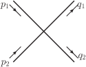
Figure 1: Lowest-order graph for 4-point Green function in $\phi^{4}$ theory, with momentum labeling appropriate for $2\to 2$ scattering.

For each propagator we have an integral of the form

$$\int\frac{\mathop{{\mathrm{d}}^{4}{}k}\nolimits}{(2\pi)^{4}}\,e^{ik\cdot(x-z)}\,\frac{i}{k^{2}-m^{2}+i\epsilon}.$$ (47)

Now, in the limit that we are interested in, the position difference $x-z$ between ends of the propagator is scaled to be large. Then for almost all values of $k$, we can deform the integration of $k$ off the real axis and get a strong suppression from the effect of the imaginary part of $k$ in the exponential. We need to determine where the deformation is not possible, and what the consequences are.

To formalize the analysis, we notate the contour deformation as

$$k=k_{R}+i\kappa k_{I}(k_{R}).$$ (48)

Here $k_{R}$ is real, $k_{I}(k_{R})$ is a real-valued function, and $\kappa$ is a parameter ranging from 0 to 1. The variable of integration is $k_{R}$. Then, given a function $k_{I}(k_{R})$ and a value of $\kappa$, Eq. (48) determines a contour of 4 real dimensions in a complex space of 8 real dimensions. Varying $\kappa$ from 0 to 1 gives a continuous family of contours, starting from an integration over all real $k$. Cauchy’s theorem tells us that the integral is independent of $\kappa$, provided that no singularities are encountered as the contour is deformed.

To get a suppression we need

$$k_{I}\cdot(x-z)>0,\quad\text{for suppression by exponential}.$$ (49)

The suppression of the integral is exponential in the large scaling of $x-z$.

However at certain points the contour deformation is obstructed by the propagator pole. At the pole, $k^{2}=m^{2}$. Suppose at some point the pole fails to obstruct the contour deformation, then at $\kappa=0$, $k_{I}$ times the derivative of $k^{2}-m^{2}$ is positive, compatible with the $i\epsilon$ prescription:

$$k_{I}^{\mu}\frac{\partial}{\partial k_{R}^{\mu}}(k_{R}^{2}-m^{2})=2k_{I}\cdot k_{R}>0,\\ \text{for non-obstruction by pole}.$$ (50)

If there exists a $k_{I}$ obeying both of conditions (49) and (50), then we can deform the contour and get an exponential suppression.

To get asymptotics of the Green function, we are interested in unsuppressed contributions, and these arise where such a $k_{I}$ fails to exist. The failure occurs when the vectors $x-z$ and $k_{R}$ are in opposite directions, i.e., when $x-z+\alpha k_{R}=0$ for some positive $\alpha$. This immediately implies that $x-z$ is time-like, since $k_{R}$ must be on-shell in order that there is a pole to obstruct the deformation.

Consider the case that $k$ is one of the incoming momenta $p_{1}$ or $p_{2}$. We already know $x-z$ is time-like for an unsuppressed contribution. Since $x$ has large negative time, $x-z$ is a time-like past-pointing vector. The non-suppression condition then states that $k_{R}$ has positive energy and is on-shell. Thus the non-suppressed contributions come from near the configuration where $k_{R}$ corresponds to propagation of a classical particle from $x$ to $z$, which is exactly what we expect for incoming asymptotic particles in a scattering process.

Similarly the asymptotic behavior when the times of $y_{1}$ and $y_{2}$ get large and positive corresponds to momenta $q_{1}$ and $q_{2}$ for outgoing classical particles.

Hence the asymptotic large-time behavior of the Green function is controlled by the poles of the propagators on the external lines, with the momenta involved being those of the appropriate classical particles. The mass of a particle is determined by the position of the pole in the propagator.

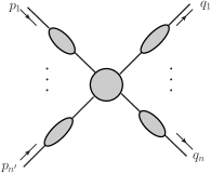
Figure 2: Graphical structure of general connected Green function with factorization of full external propagators, with momentum labeling appropriate for $n^{\prime}\to n$ scattering.

This idea generalizes readily. In Fig. 2 the connected part of an $n+n^{\prime}$-point Green function is decomposed into the product of an amputated part and full propagators for each external line. Generally a full propagator with momentum $k$ has not only a particle pole, but a set of other, weaker, singularities at higher values of $k^{2}$ that are thresholds for $k$ to make multiple particles. The dominant large time behavior is governed by the strongest singularity, i.e., the particle pole.

VI Källen-Lehmann representation

The Källen-Lehmann representation [28, 29] (or “spectral representation”) is important to the general analysis of the 2-point function, and to the generality of the correspondence between single-particle states and the positions of poles of 2-point functions in momentum space. More detailed treatments can be found in many textbooks on QFT, and I will only summarize here the results needed for this paper.

The Källen-Lehmann representation concerns the 2-field correlator:

$$\langle 0|\phi(x)\phi(y)|0\rangle,$$ (51)

and it is obtained by inserting a complete set of in- or out-basis states between the two fields and by using the fact that for a state $|p\rangle$ of 4-momentum $p$, the $x$ dependence of $\langle 0|\phi(x)|p\rangle$ obeys

$$\langle 0|\phi(x)|p\rangle=\langle 0|\phi(0)|p\rangle e^{-ip\cdot x}.$$ (52)

Both of the time-ordered propagator and the vacuum expectation value of equal-time commutators (and non-equal-time commutators) can be obtained from (51). All of these are expressed in terms of a non-negative spectral function $\rho(s)$ which measures the size of $\left|\langle 0|\phi|p\rangle\right|^{2}$ for states of invariant squared mass $s$, and is defined by

$$\rho(s)\stackrel{{\scriptstyle\textrm{def}}}{{=}}(2\pi)^{3}\sum_{X}\delta^{(4)}(p_{X}-p_{s})|\langle 0|\phi(0)|X\rangle|^{2},$$ (53)

where $\sum_{X}$ denotes a sum/integral over a complete set of 4-momentum eigenstates (which can be chosen to be the out-basis states or the in-basis states), $p_{X}$ is the 4-momentum of $|X\rangle$, and $p_{s}$ is a vector obeying $p_{s}^{2}=s$ and having a positive energy component.

We can now express the 2-field correlator in terms of a free field correlator:

$$\langle 0|\phi(x)\phi(y)|0\rangle =\int_{0}^{\infty}\mathop{{\mathrm{d}}{}s}\nolimits\rho(s)\,\Delta((x-y)^{2};s)$$

$$=\int_{0}^{\infty}\mathop{{\mathrm{d}}{}s}\nolimits\rho(s)\,\int\frac{\mathop{{\mathrm{d}}^{3}{}\boldsymbol{k}}\nolimits}{(2\pi)^{3}2\sqrt{\boldsymbol{k}^{2}+s}}e^{-ik\cdot(x-y)},$$

$$=\int\frac{\mathop{{\mathrm{d}}^{4}{}k}\nolimits}{(2\pi)^{3}}\rho(k^{2})\theta(k^{0})e^{-ik\cdot(x-y)},$$ (54)

where in the exponent on the second line $k^{0}=\sqrt{\boldsymbol{k}^{2}+s}$. The quantity $\Delta((x-y)^{2};s)$ is the correlator (51) for the case of a free field of mass $\sqrt{s}$, which for space-like $x-y$ is in terms of a particular Bessel function (e.g., Ref. [30]):

$$\Delta((x-y)^{2};s)=\frac{\sqrt{s}}{4\pi^{2}\sqrt{-(x-y)^{2}}}K_{1}\mathopen{}\left(\sqrt{-s(x-y)^{2}}\right)\\ ~{}\mbox{for space-like $x-y$}.$$ (55)

It then follows that the propagator, i.e., the Fourier transform of the time-ordered version of the correlator, is

$$\hat{G}_{2}(p^{2})=\int_{0}^{\infty}\mathop{{\mathrm{d}}{}s}\nolimits\rho(s)\,\frac{i}{p^{2}-s+i\epsilon}.$$ (56)

Suppose that the field has a non-zero matrix element between the vacuum and a single particle state:

$$\langle 0|\phi(x)|\boldsymbol{p}\rangle=c\,e^{-ip\cdot x},$$ (57)

where $p^{0}=E_{\boldsymbol{p}}=\sqrt{\boldsymbol{p}^{2}+m_{\rm phys}^{2}}$, and $m_{\rm phys}$ is the physical mass of the particle. Then there is a contribution to $\rho(s)$ of the form $|c|^{2}\delta(s-m_{\rm phys}^{2})$. All other contributions are from continuum parts of the allowed energies, and start at higher particle thresholds; they give no further delta functions. Hence the propagator has a pole with residue $|c|^{2}$ at $p^{2}=m_{\rm phys}^{2}$:

$$\hat{G}_{2}(p^{2})=\frac{i|c|^{2}}{p^{2}-m_{\rm phys}^{2}+i\epsilon}+\mbox{non-pole term}.$$ (58)

We write the residue as $R=|c|^{2}$.

Commonly one normalizes the single-particle states to make $c$ real and positive. But this is only possible in one matrix element like (57). If we examine 2-point functions for this and other fields that have nonzero coupling between the vacuum and the single-particle state, then $c$ is normally different in each case and can only be normalized to be real and positive for one of them.

VII Space-time wave functions

Since space-time localization is important, let us define a coordinate-space wave function for each particle in states such as those in Eqs. (35) and (38), by writing

$$f(x)=f(t,\boldsymbol{x}) \stackrel{{\scriptstyle\textrm{def}}}{{=}}\int\mathop{\widetilde{\mathop{{\mathrm{d}}{}p}\nolimits}}\nolimits\tilde{f}(\boldsymbol{p})\,e^{-ip\cdot x}$$

$$=\int\mathop{\widetilde{\mathop{{\mathrm{d}}{}p}\nolimits}}\nolimits\tilde{f}(\boldsymbol{p})\,e^{-iE_{\boldsymbol{p}}t+i\boldsymbol{p}\cdot\boldsymbol{x}},$$ (59)

where $f$ corresponds to any of the $f_{j}$ or $g(x)$. Here $p$ is on shell, of course, at the physical particle mass. Each of these wave functions is a function of time and spatial position. It is thus like an ordinary Schrödinger wave function in the non-relativistic quantum mechanics of a single particle.

Although, in general, there are great difficulties in using wave functions in relativistic theories with interactions, the concept of a wave function is valid in a free-field theory, for the state of one particle. Our use of wave functions is as useful auxiliary quantities, in the analysis of a state in terms of its particle content in the infinite past or future, where the state corresponds to a set of isolated particles. That is, we use the concept of wave function only for the center-of-mass motion of a single particle and then only when the particle is being correctly approximated as a free particle. (Since it is the center-of-mass motion that is relevant here, these ideas apply equally when the particle is a bound state of more elementary constituents.)

Unlike the case of multiparticle wave functions in non-relativistic quantum mechanics, we do not assign a common time variable to all the single-particle wave functions for a state of multiple particles. The purpose of our wave functions is not the one used in non-relativistic quantum mechanics, where time-dependent wave functions implement time-dependent states in the Schrödinger picture. Here their purpose is to simply give a useful quantity with which to analyze the relation between the states in Eqs. (35) and (38), the S-matrix, and certain matrix elements involving the Heisenberg-picture field operators.

In basic applications to scattering, we assume that the momentum-space wave functions are sharply peaked about one momentum. Then the coordinate-space wave functions describe propagating wave packets, as will now verify. Thus they correspond to propagation of free particles with approximately definite momenta. For analyzing scattering processes, we will need information about the asymptotic behavior of wave functions in coordinate space for large positive and negative times.

Consider a momentum-space wave function that is sharply peaked around one value of momentum, $\boldsymbol{p}_{0}$, and that has a width characterized by one number $\Delta p$. We will initially choose the wave function also to be real and non-negative. One simply possibility would be a Gaussian

$$f(\boldsymbol{p};\boldsymbol{p}_{0},\Delta p)\stackrel{{\scriptstyle\textrm{?}}}{{=}}De^{-(\boldsymbol{p}-\boldsymbol{p}_{0})^{2}/\Delta p^{2}},$$ (60)

with $D$ adjusted to give unit normalization:

$$\int\mathop{\widetilde{\mathop{{\mathrm{d}}{}p}\nolimits}}\nolimits|f(\boldsymbol{p})|^{2}=1.$$ (61)

However, this has a (small) tail extending out to infinite momentum. For reasons to be reviewed below, this gives large-time behavior that is not quite optimal for constructing a proof of the reduction formula. Therefore [6, 7] it is better to choose a wave function of compact support, i.e., one that vanishes outside a finite range of $\boldsymbol{p}$. One simple possibility would be the infinitely differentiable function

$$f(\boldsymbol{p};\boldsymbol{p}_{0},\Delta p)=\begin{cases}De^{-1/(1-|\boldsymbol{p}-\boldsymbol{p}_{0}|^{2}/\Delta p^{2})}&\mbox{if $|\boldsymbol{p}_{0}-\boldsymbol{p}|<\Delta p$},\\ 0&\mbox{if $|\boldsymbol{p}_{0}-\boldsymbol{p}|\geq\Delta p$},\end{cases}$$ (62)

with $D$ being again adjusted to give a normalized wave function, (61).

The corresponding coordinate-space wave function, from Eq. (VII), is of maximum size at the origin, i.e., when $x=0$. This is because at that point, the integrand is strictly positive. At all other values of $x$, the phase factor $e^{-iE_{\boldsymbol{p}}t+i\boldsymbol{p}\cdot\boldsymbol{x}}$ is not always unity, and therefore there are some cancellations.

VII.1 Properties needed

For a treatment of scattering theory and a derivation of the S-matrix, we need to know roughly the behavior of single-particle wave functions in coordinate space. In the derivation, we will encounter integrals of coordinate-space wave functions multiplied by Green functions, as in Eq. (136), in which certain ranges of time are selected. We will need to understand which regions of the integrals over spatial coordinates give non-zero contributions in a limit of infinite time and which regions give asymptotically vanishing contributions, and to see that the asymptotic space-time structure does in fact corresponding to the expected scattering phenomena.

To this end, suppose we are given a wave function obeying the properties given just above. Then we need estimates of the following:

1. The location in $\boldsymbol{x}$ of the peak of the wave function, for a given value of $t$.

2. The corresponding width in $\boldsymbol{x}$.

3. The asymptotic behavior when $t$ goes to infinity (or negative infinity), as a function of $\boldsymbol{x}$. This is especially needed for the asymptotic behavior far from the peak of the wave function.

However, only rough estimates will be needed.

When related to our use of $f(x)$ in QFT, the location of the peak verifies that the particle propagates classically. The width of the peak quantifies the inaccuracy of a purely classical view; in a scattering situation, the width determines when and where the different particles in the initial or final states can start to be regarded as separate non-interacting particles. The asymptotic behavior is needed to ensure that asymptotically the particles are cleanly separated; it is here that the motivation will arise to use wave functions of compact support in momentum space.

If we use a momentum-space wave function of a form such as is defined in (60) or (62), we will find that the classical trajectory of the particle goes through the origin of spatial coordinates at time zero, and also has minimum width there. Of course, we need to allow more general possibilities for the trajectory; this is easily done by applying a space-time translation — see Sec. VII.6 below.

VII.2 Stationary phase

The integrand in (VII) for the coordinate-space wave function is a real, positive factor multiplied by the phase $e^{-iE_{\boldsymbol{p}}t+i\boldsymbol{p}\cdot\boldsymbol{x}}$. Suppose that $t$ and/or $\boldsymbol{x}$ is made large. Then the integrand, as a function of $\boldsymbol{p}$, generally has rapid oscillations, which result in a small contribution to $f(x)$. Given a particular value of time $t$, if $\boldsymbol{x}$ is increased sufficiently, then for most values of $\boldsymbol{p}$ the oscillations become arbitrarily rapid, and the corresponding contribution to $f(x)$ decreases rapidly to zero, i.e., faster than any power of $\boldsymbol{x}$, by a standard theorem.

The exception to these statements occurs where there is a lack of oscillations, i.e., at and close to the point of stationary phase. Given a value of $t$ and $\boldsymbol{x}$, the stationary-phase point is the value $\boldsymbol{p}_{\rm c}$ where

$$0=\frac{\partial(-E_{\boldsymbol{p}_{\rm c}}t+\boldsymbol{p}_{\rm c}\cdot\boldsymbol{x})}{\partial\boldsymbol{p}_{\rm c}}=-\frac{\boldsymbol{p}_{\rm c}t}{E_{\boldsymbol{p}_{\rm c}}}+\boldsymbol{x},$$ (63)

i.e.,

$$\boldsymbol{p}_{\rm c}=\frac{m\boldsymbol{x}\operatorname{sign}{t}}{\sqrt{t^{2}-\boldsymbol{x}^{2}}},$$ (64)

so that

$$E_{\boldsymbol{p}_{\rm c}}=\frac{m|t|}{\sqrt{t^{2}-\boldsymbol{x}^{2}}},$$ (65)

Notice that the stationary phase condition only has a solution when $x=(t,\boldsymbol{x})$ is time-like or zero.

Now let use restrict to the case that $\tilde{f}(\boldsymbol{p})$ is like the examples in (60) or (62), i.e., real, non-negative, and strongly peaked at one value $\boldsymbol{p}=\boldsymbol{p}_{0}$. Then, given $t$, the coordinate-space wave function is largest when the stationary phase point is close to the maximum of the function $\tilde{f}(\boldsymbol{p})$, i.e., when $\boldsymbol{p}_{\rm c}=\boldsymbol{p}_{0}$, and thus when

$$\boldsymbol{x}\simeq\frac{\boldsymbol{p}_{0}t}{E_{\boldsymbol{p}_{0}}}=\boldsymbol{v}_{0}t.$$ (66)

This is the trajectory of a classical relativistic particle, which therefore, as expected, matches the overall propagation of the wave packet. The 3-velocity is $\boldsymbol{v}_{0}=\boldsymbol{p}_{0}/E_{\boldsymbol{p}_{0}}$.

VII.3 Width

For the analysis of the width of the coordinate-space wave function in coordinate space for a given $t$, we still consider cases with momentum-space wave functions like those in (60) or (62). First consider $t=0$. The peak of the wave function is at the origin, $\boldsymbol{x}=0$. As $\boldsymbol{x}$ moves away from this position, we reach a situation when about one oscillation of the $e^{i\boldsymbol{p}\cdot\boldsymbol{x}}$ factor as a function of $\boldsymbol{p}$ fits inside the peak of the momentum-space wave function. Hence the width of the wave function is of order $1/\Delta p$. We can call this the uncertainty-principle value or the quantum mechanical uncertainty.

When $|t|$ is increased sufficiently much away from zero, the oscillations in $e^{-iE_{\boldsymbol{p}}t}$ are important. For determining the width of the wave function, these first become significant when there is a change of order unity in the phase when one moves from $\boldsymbol{p}=\boldsymbol{p}_{0}$ to a value differing by $\Delta p$. We estimate where this happens by using the derivative of $E_{\boldsymbol{p}}$ at $\boldsymbol{p}_{0}$ and our general assumption that $\Delta p$ is small. Then the uncertainty-principle estimate continues to apply when

$$|t|\lesssim\frac{E_{\boldsymbol{p}_{0}}}{\Delta p(|\boldsymbol{p}_{0}|+\Delta p)}.$$ (67)

Notice that if $\Delta p$ is very small, this is a large range of times. But always, for a given wave function, once $t$ gets large enough in size, positive or negative, the uncertainty principle uncertainty is insufficient.

At large enough values of time, it is the stationary phase point given in (64) that is relevant. The size of the coordinate-space wave function corresponds to the size of the $\tilde{f}(\boldsymbol{p})$ at $\boldsymbol{p}=\boldsymbol{p}_{\rm c}$. This is multiplied by an overall $t$-independent factor from the integration measure, and by a factor with power-law $t$ dependence. The second factor can be estimated asymptotically by expanding the exponent of the phase factor to second order in momentum about $\boldsymbol{p}=\boldsymbol{p}_{\rm c}$, and doing a saddle point expansion.

Hence, for large enough $|t|$, the width of the wave function is determined by where the stationary phase point deviates from the central value of momentum by $\Delta p$. That is it is determined by where $|\boldsymbol{p}_{\rm c}(t,\boldsymbol{x})-\boldsymbol{p}_{0}|=O(\Delta p)$. To understand what this implies for where in $\boldsymbol{x}$, the coordinate-space wave function starts to fall off, we start with a value of $\boldsymbol{p}_{\rm c}$ obeying the last condition, and compute the corresponding value of $\boldsymbol{x}=\boldsymbol{p}_{\rm c}t/E_{\boldsymbol{p}_{\rm c}}$. This corresponds to the propagation of a classical particle of momentum $\boldsymbol{p}_{\rm c}$. In this situation of large enough $|t|$, the width of the wave function therefore corresponds to classical dispersion, i.e., to the different velocities of classical particles of different momenta. The dependence of this contribution on the width, as a function of $\Delta p$ and $t$, is completely different to that of the quantum uncertainty-principle width. It increases proportionally to $t$, whereas the uncertainty-principle is independent of time. Moreover it is proportional to $\Delta p$, decreasing to zero when $\Delta p\to 0$. In contrast, the uncertainty principle width is of order $1/\Delta p$ and becomes infinite when $\Delta p\to 0$.

An appropriate estimate for the order of magnitude of the width is simply to add the uncertainty-principle and classical-dispersion widths or to add them in quadrature.

VII.4 Asymptote

We now evaluate the asymptotics of the wave function as $t\to\pm\infty$. If $(t,\boldsymbol{x})$ is time like, then the wave function’s value is dominated by an integral near the corresponding stationary phase point $\boldsymbol{p}_{\rm c}$. This is multiplied by a power law in $t$. When $(t,\boldsymbol{x})$ is space-like, there is no stationary-phase point and hence the coordinate-space wave function falls off faster than any power of $t$ (for a fixed ratio $\boldsymbol{x}/t$), as follows from standard properties of Fourier transforms of infinitely differentiable functions.

For time-like $(t,\boldsymbol{x})$, the leading asymptote is given by a Gaussian approximation around the stationary-phase point, as I now show. Let $\delta\boldsymbol{p}=\boldsymbol{p}-\boldsymbol{p}_{\rm c}$, with $\boldsymbol{p}_{\rm c}$ given by Eq. (64), and let $\delta p_{\|}$ and $\delta\boldsymbol{p}_{\perp}$ be the components of $\delta\boldsymbol{p}$ parallel and perpendicular to $\boldsymbol{p}_{\rm c}$. Then the exponent in Eq. (VII) is

$$-iE_{\boldsymbol{p}}t+i\boldsymbol{p}\cdot\boldsymbol{x}= -im\sqrt{t^{2}-\boldsymbol{x}^{2}}$$

$$-i\frac{\delta p_{\|}^{2}(t^{2}-\boldsymbol{x}^{2})^{3/2}}{2mt^{2}}-i\frac{\delta p_{\perp}^{2}(t^{2}-\boldsymbol{x}^{2})^{1/2}}{2m}$$

$$+\dots,$$ (68)

where the cubic and higher terms indicated by $\dots$ are suppressed by a power of $|\delta\boldsymbol{p}|/E_{\boldsymbol{p}_{\rm c}}$ relative to the quadratic term.

We can deform the integrals over $\delta p_{\|}$ and $\delta\boldsymbol{p}_{\perp}$ into the complex plane to go down the directions of steepest descent. For large $|t|$, the integral is dominated by $\delta\boldsymbol{p}$ of order $1/t$. More exactly, the dominance is by $\delta p_{\|}$ of order $\sqrt{m}t(t^{2}-\boldsymbol{x}^{2})^{-3/4}$ and $\delta p_{\perp}$ of order $\sqrt{m}(t^{2}-\boldsymbol{x}^{2})^{-1/4}$. We can use a Gaussian approximation to estimate $f(x)$:

$$f(x)\sim \frac{\tilde{f}(\boldsymbol{p}_{\rm c})e^{-3\pi i/4}m^{3/2}}{(2\pi)^{3}2E_{\boldsymbol{p}_{\rm c}}}e^{-i\sqrt{t^{2}-\boldsymbol{x}^{2}}}\frac{t}{(t^{2}-\boldsymbol{x}^{2})^{5/4}}$$

$$= \frac{\tilde{f}(\boldsymbol{p}_{\rm c})e^{-3\pi i/4}E_{\boldsymbol{p}_{\rm c}}^{3/2}}{(2\pi)^{3}2m}\,\frac{e^{-i\sqrt{t^{2}-\boldsymbol{x}^{2}}}\operatorname{sign}t}{|t|^{3/2}},$$ (69)

with errors suppressed by a power of $1/t$. There is implicit dependence on $\boldsymbol{x}$ and $t$, in the dependence on $\boldsymbol{p}_{\rm c}$, since $\boldsymbol{p}_{\rm c}=m(\boldsymbol{x}/t)/\sqrt{1-\boldsymbol{x}^{2}/t^{2}}$, but this is only a dependence on the ratio $\boldsymbol{x}/t$, i.e., a velocity. By inverting the relationship of $\boldsymbol{p}_{\rm c}$ to $\boldsymbol{x}/t$, we see that the momentum-space wave function $\tilde{f}(\boldsymbol{p})$ at a particular value of momentum gives a contribution to the asymptote of $f(x)$ at a corresponding value of velocity

$$\frac{\boldsymbol{x}}{t}=\frac{\boldsymbol{p}}{E_{\boldsymbol{p}}}=\frac{\boldsymbol{p}}{\sqrt{m^{2}+\boldsymbol{p}^{2}}},$$ (70)

which is of course the well-known value for the relativistic propagation of a classical particle.

At fixed velocity $\boldsymbol{x}/t$, Eq. (VII.4) shows that $f(x)$ decreases like $1/|t|^{3/2}$ at large $t$. When we construct the S-matrix, it will be the $1/|t|^{3/2}$ asymptote that gives the S-matrix; weaker contributions to $f(x)$ are irrelevant to the S-matrix.

Figure 3: Illustrating space-time evolution of wave function $f(t,\boldsymbol{x})$. The horizontal lines indicate at particular times the width of the wave packet.

VII.5 Asymptote for compact support momentum-space wave function

Some simplifications occur if the momentum-space wave function has compact support, i.e., if it vanishes outside a finite range of $\boldsymbol{p}$. Then, for the coordinate-space wave function, the range of velocities $\boldsymbol{x}/t$ for which applies the $1/|t|^{3/2}$ decrease is equally compact, i.e., bounded. Outside this range, $f(x)$ decreases more rapidly with $t$. This provides a useful visualizable localization, as in Fig. 3. For a given large value of $|t|$, the range of $\boldsymbol{x}$ in which the $1/|t|^{3/2}$ decrease applies has a volume of order $|t|^{3}$.

The space of functions of compact support is dense in the space of normalizable wave functions, so we have no loss of generality if we restrict attention to wave functions of compact support in momentum space.

In contrast it is not particularly useful to impose a condition of compact support in spatial position on the coordinate-space wave function. To see this, observe that if a function of $\boldsymbol{x}$ has compact support, then its Fourier transform into $\boldsymbol{p}$ space can be continued to all complex $\boldsymbol{p}$ and is analytic everywhere. Conversely, if there is a singularity of the Fourier transform for some value of $\boldsymbol{p}$, then the original function of $\boldsymbol{x}$ cannot be of compact support. Now suppose, the wave function $f(x)$ in (VII) is of compact support in $\boldsymbol{x}$ for one value of $t$, say $t=t_{0}$. Then $\tilde{f}(\boldsymbol{p})\,e^{-iE_{\boldsymbol{p}}t_{0}}/E_{\boldsymbol{p}}$ is analytic for all complex $\boldsymbol{p}$. Going to another value of $t$ gives an extra factor $e^{-iE_{\boldsymbol{p}}(t-t_{0})}$ on the right-hand side of (VII). This is not analytic, because it has a singularity where $\boldsymbol{p}^{2}=-m_{\rm phys}^{2}$, and hence $f(t,\boldsymbol{x})$ is not of compact support in $\boldsymbol{x}$. Thus a condition of compact support in space can be maintained for at most one instant in time.

VII.6 Shift of wave function in coordinate space

We now ask how to shift the wave, so that the classical trajectory is

$$\boldsymbol{x}\simeq\boldsymbol{x}_{a}+\boldsymbol{v}_{0}(t-t_{a}),$$ (71)

so that instead of occurring at the origin, the minimum width occurs at time $t_{a}$, with the position of the particle at that time being $\boldsymbol{x}_{a}$. This is done by multiplying the momentum-space wave function by a suitable phase. We replace $f(\boldsymbol{p};\boldsymbol{p}_{0},\Delta p)$ by

$$f(\boldsymbol{p};\boldsymbol{p}_{0},\Delta p)\mapsto f(\boldsymbol{p};\boldsymbol{p}_{0},\Delta p)e^{iE_{\boldsymbol{p}}t_{a}-\boldsymbol{p}\cdot\boldsymbol{x}_{a}}.$$ (72)

Then the coordinate-space wave function gets changed by

$$f(t,\boldsymbol{x})\mapsto f(t-t_{a},\boldsymbol{x}-\boldsymbol{x}_{a}),$$ (73)

as can be verified by substituting the modified momentum-space wave function in the defining formula (VII) for the coordinate-space wave function.

VIII The reduction formula

In this section, I state the reduction formula, of which an improved proof will be in Sec. XI. It is useful to focus attention separately on the connected components of the Green functions (and hence of the S-matrix). It is the fully connected term that is relevant to standard calculations, and we will focus exclusively on that in this section.

Let $\tilde{G}_{N}^{\text{conn}}(p_{1},p_{2},\dots p_{N})$ be a connected $N$-point Green function, and let $\Gamma_{N}(p_{1},p_{2},\dots p_{N-1})(2\pi)^{4}\delta^{(4)}(p_{1}+\dots+p_{N})$ be the corresponding amputated Green function. It is convenient to choose $\Gamma_{N}$ to be defined without the momentum conservation delta function. So it only has $N-1$ independent momentum arguments, and the last momentum obeys $p_{N}=-\sum_{j=1}^{N-1}p_{j}$. We choose the convention for the arguments of Green functions that all the momenta flow in.

The unamputated and amputated Green functions are related by

$$\tilde{G}_{N}^{\text{conn}}(p_{1},p_{2},\dots p_{N})=\prod_{j=1}^{N}\hat{G}_{2}(p_{j}^{2})\,\,\Gamma_{N}(p_{1},p_{2},\dots p_{N-1})(2\pi)^{4}\delta^{(4)}(p_{1}+\dots+p_{N}),$$ (74)

where $\hat{G}_{2}(p^{2})$ is the propagator, i.e., the 2-point function without its momentum-conservation delta function. Let $c$ be the coefficient in the normalization of the vacuum-to-one-particle matrix element, as in Eq. (57). Then, as seen at Eq. (58), the propagator has a pole at the physical mass of the particle and the propagator residue is $R=|c|^{2}$.

The LSZ theorem [1] both states that the wave packet states $\langle g_{1},\dots,g_{n};\,{\rm out}|f_{1},\dots,f_{n^{\prime}};\,{\rm in}\rangle$ have the form (39) and states how the S-matrix is given in terms of Green functions. The LSZ result for the connected part of the S-matrix element for $n^{\prime}\to n$ scattering is

$$S^{\text{conn}}_{\boldsymbol{q}_{1},\dots\boldsymbol{q}_{n};\,\boldsymbol{p}_{1},\dots\boldsymbol{p}_{n^{\prime}}}=\lim_{\rm on-shell}\frac{1}{c^{n}(c^{*})^{n^{\prime}}}\,\prod_{k=1}^{n}\frac{q_{j}^{2}-m_{\rm phys}^{2}}{i}\,\,\prod_{j=1}^{n^{\prime}}\frac{p_{j}^{2}-m_{\rm phys}^{2}}{i}\,\,\tilde{G}_{n+n^{\prime}}^{\text{conn}}(p_{1},\dots,p_{n^{\prime}},-q_{1},\dots-q_{n-1}).$$ (75)

Observe that the full Green function $\tilde{G}_{n+n^{\prime}}$ diverges when the external momenta are put on-shell. This formula asserts that the S-matrix is obtained by first multiplying the Green function by the factors of $p_{j}^{2}-m_{\rm phys}^{2}$, etc, to cancel the poles, and by then taking the limit of on-shell momenta, and finally by inserting the factor $1/(c^{n}(c^{*})^{n^{\prime}})$. An important and non-trivial part of (75) is this last factor, which involves the normalization of the vacuum-to-one-particle of the field. In the usual case that $c$ is real and positive, the factor equals $1/R^{(n+n^{\prime})/2}$, where $R$ is the residue of the pole in the full propagator.

A convenient version of the reduction formula is in terms of the amputated Green function:

$$S^{\text{conn}}_{\boldsymbol{q}_{1},\dots\boldsymbol{q}_{n};\,\boldsymbol{p}_{1},\dots,\boldsymbol{p}_{n^{\prime}}}=(2\pi)^{4}\delta^{(4)}\left({\textstyle\sum}_{j=1}^{n^{\prime}}p_{j}-{\textstyle\sum}_{k=1}^{n}q_{k}\right)\,(c^{*})^{n}c^{n^{\prime}}\,\Gamma_{n+n^{\prime}}(p_{1},\dots,p_{n^{\prime}},-q_{1},\dots-q_{n-1})\,.$$ (76)

Here the external momenta of the amputated Green function are set on shell from the beginning. This formula gives the following procedure for computing the S-matrix:

1. Replace each full external propagator of the full Green function by the factor $c$ for incoming lines and $c^{*}$ for outgoing lines.

2. Set the external momenta on-shell.

The actual statement of the theorem by LSZ was for the case that the vacuum-field-particle matrix element had unit normalization, i.e., $c=1$. But it is elementary to extend the theorem to where $c\neq 1$, as can be seen in many textbooks, e.g., [31, 21, 23, 22]. LSZ presented their result in a different but equivalent form to that given here. Their formula is obtained from Eq. (39) by substituting Eq. (75) for the S-matrix and then expressing the momentum-space Green function in terms of the corresponding coordinate-space Green function. It is quite elementary to reverse the procedure, i.e., to perform the Fourier transforms in LSZ’s actual formula to obtain the combination of Eqs. (39) and (75). Many, but not all, authors do present the momentum-space form that is relevant for actual calculations.

A simple extension to matrix elements of operators between in and out states is also elementary — see p. 53 of [21]. Such matrix elements have the form

$$\langle\alpha;\,{\rm out}|\,T\,\text{operator(s)}\,|\beta;\,{\rm in}\rangle.$$ (77)

Cases in regular use are where operators are currents in QCD and the matrix elements are for the hadronic part of scattering amplitudes or cross sections that involve both QCD and the electroweak interactions, e.g., deeply inelastic scattering and the Drell-Yan process.

Practical calculations involve on-shell amputated Green functions and a separate calculation of the physical mass and the propagator residue. Direct calculations of perturbative corrections to the propagator are not useful in themselves because they give terms with higher-order poles, from two or more free propagators in series, e.g., Fig. 4. This results in non-convergence of the sum when the momentum is near the particle pole.

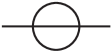
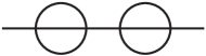
Figure 4: Propagator corrections.

This problem is evaded by a resummation in terms of the self-energy function $\Sigma(p^{2},m_{R},\lambda_{R})$, which is defined to be $i$ times a 2-point Green function that is irreducible in the external line; it includes any necessary renormalization counterterms. It is analytic when $p^{2}$ is in a neighborhood of its on-shell value. I have written $\Sigma(p^{2},m_{R},\lambda_{R})$ with explicit arguments for renormalized mass and coupling. In many schemes there is also a renormalization mass $\mu$, but I have left that argument implicit. There is no requirement for the renormalized mass to equal the physical mass.

In terms of the self-energy, the propagator is

$$\hat{G}_{2}(p^{2})=\frac{i}{p^{2}-m_{R}^{2}-\Sigma(p^{2},m_{R},\lambda_{R})+i\epsilon}.$$ (78)

The physical mass can be determined in terms of the parameters of the theory, i.e., the renormalized mass and coupling, by solving

$$m_{\rm phys}^{2}-m_{R}^{2}-\Sigma(m_{\rm phys}^{2},m_{R},\lambda_{R})=0,$$ (79)

which can be done order-by-order in perturbation theory. The propagator’s residue is then

$$R=\left.\frac{1}{1\mathbin{-}\partial\Sigma(p^{2})/\partial p^{2}}\right|_{p^{2}=m_{\rm phys}^{2}},$$ (80)

which is also susceptible to perturbative calculation.

IX Creation of in- and out-states by fields

In Eqs. (35) and (38), we proposed states $|f_{1},f_{2};\,{\rm in}\rangle$ and $|g_{1},\dots;\,{\rm out}\rangle$ that have simple expressions when parameterized by what we termed momentum-space wave functions: $\tilde{f}_{j}(\boldsymbol{p})$, etc.

For all our considerations concerning scattering, we assume that each momentum-space wave function is peaked around a particular value of momentum. Since the space spanned by such functions is the whole space of wave functions, this condition will not give any loss of generality. But it will enable arguments concerning scattering to be visualizable.

The state $|f_{1},f_{2};\,{\rm in}\rangle$ is intended to be a state which at very large negative times approaches a state of free separated individual particles with wave function $\tilde{f}_{1}(\boldsymbol{p}_{1})\,\tilde{f}_{2}(\boldsymbol{p}_{2})$. The simplest case to understand is when, following Sec. VII.5, we choose $\tilde{f}_{1}$ and $\tilde{f}_{2}$ to be of compact support, and also choose them to have non-overlapping supports. In this case, we have non-overlap of the region of asymptotic $1/|t|^{3/2}$ decrease of the corresponding coordinate space wave functions. It is the region of $1/|t|^{3/2}$ decrease that matters, because that is the part that is relevant for obtaining the S-matrix. In the non-overlapping case, the regions of $1/|t|^{3/2}$ decrease for $f_{1}$ and $f_{2}$ are space-like separated for a given large enough value of $t$ (positive or negative), and then the particles are causally separated.

When we go to the more general overlapping case, a somewhat less trivial argument is needed to show that the two particles do not causally influence each other. Our proof of the reduction formula will be organized in such a way that the issue of separation of the different particles at infinite time is handled rather indirectly.

Similar statements apply to the state $|g_{1},\dots;\,{\rm out}\rangle$, except that they are applied in the far future. Exactly how far one has to go to the past and future to have a good free-particle approximation depends on the state, i.e., on the wave functions.

The aim of this section is to construct creation operators that genuinely create single asymptotic particles in the far past and future. The complication we will need to overcome is that, as we will see, the simplest and natural candidate definition for these operators, i.e., the one used by LSZ, gives operators that create much more than the intended single particles. The new operators will then be used in a proof of the reduction formula. Separately, after the proof is completed, we will be able to verify not only the property inherent in the definition that one creation operator applied to the vacuum creates the intended single particle, but also that multiple applications of the operator create the intended multiparticle state and nothing else.

The starting point consists of the following assumptions (a) that we have a QFT that exists and that obeys standard principles; (b) that it has a scattering theory that obeys the principles given in Sec. IV; and (c) that there is a nonzero vacuum-to-one-particle matrix element of the field $\phi(x)$. Poincaré invariance is assumed, as usual, but that assumption can be relaxed, normally with a penalty only in notational complexity.

I will first demonstrate by explicit perturbative calculations the already-summarized problem that the LSZ creation operators $a_{f}^{\dagger}(t)$ create much more than the desired single particles, and that the limits as $t\to\pm\infty$ do not help. Because the field operators in the defining formula for $a_{f}^{\dagger}(t)$ are at fixed time, there is effectively an infinite uncertainty in energy, with the corresponding possibility of creating arbitrarily many particles.

With the results of those calculations as motivation, I will then give a suitable definition of creation operators. It modifies the LSZ definition by applying a time average.

IX.1 Free fields

We start with a review of the case of a free field theory, without interactions. With the standard normalization, the Lagrangian density is

$$\mathcal{L}=\frac{1}{2}(\partial\phi_{{\rm free}})^{2}-\frac{m^{2}}{2}\phi_{{\rm free}}^{2}.$$ (81)

The standard expansion of the field in terms of time-independent creation and annihilation operators was given in Eq. (5). These operators can be found in terms of the field $\phi_{{\rm free}}(t,\boldsymbol{x})$ and the canonical momentum field $\pi_{{\rm free}}(t,\boldsymbol{x})=\partial\phi_{{\rm free}}/\partial t$ at fixed time:

$$a_{\boldsymbol{k},{\rm free}}^{\dagger} =\int\mathop{{\mathrm{d}}^{3}{}\boldsymbol{x}}\nolimits e^{-ik\cdot x}\left[E_{\boldsymbol{k}}\phi_{{\rm free}}(x)-i\pi_{{\rm free}}(x)\right],$$ (82a)

$$a_{\boldsymbol{k},{\rm free}} =\int\mathop{{\mathrm{d}}^{3}{}\boldsymbol{x}}\nolimits e^{ik\cdot x}\left[E_{\boldsymbol{k}}\phi_{{\rm free}}(x)+i\pi_{{\rm free}}(x)\right],$$ (82b)

where $k^{\mu}=\left(\sqrt{\boldsymbol{k}^{2}+m^{2}},\boldsymbol{k}\right)$. The $\phi$ and $\pi$ fields are important because they are the independent fields that appear in the Hamiltonian. From the equal-time commutation relations, and specifically $[\phi_{{\rm free}}(t,\boldsymbol{x}),\pi_{{\rm free}}(t,\boldsymbol{y})]=i\delta^{(3)}(\boldsymbol{x}-\boldsymbol{y})$, follow the standard commutation relations, (2), for the annihilation and creation operators. Given that $a_{\boldsymbol{k},{\rm free}}$ annihilates the vacuum, i.e., $a_{\boldsymbol{k},{\rm free}}|0,{\rm free}\rangle=0$, all the usual consequences follow.

A generic normalizable one-particle state is

$$|f;{\rm free}\rangle={} \int\mathop{\widetilde{\mathop{{\mathrm{d}}{}p}\nolimits}}\nolimits\,|\boldsymbol{p};{\rm free}\rangle\,\tilde{f}(\boldsymbol{p})$$

$$={} \int\mathop{\widetilde{\mathop{{\mathrm{d}}{}p}\nolimits}}\nolimits\,a_{\boldsymbol{p},{\rm free}}^{{\dagger}}\,|0;{\rm free}\rangle\,\tilde{f}(\boldsymbol{p}).$$ (83)

It is useful to define creation and annihilation operators corresponding to this state by

$$a_{f,{\rm free}}^{\dagger}\stackrel{{\scriptstyle\textrm{def}}}{{=}}\int\mathop{\widetilde{\mathop{{\mathrm{d}}{}k}\nolimits}}\nolimits\tilde{f}(\boldsymbol{k})\,a_{\boldsymbol{k}}^{\dagger},\quad a_{f,{\rm free}}=\int\mathop{\widetilde{\mathop{{\mathrm{d}}{}k}\nolimits}}\nolimits\tilde{f}^{*}(\boldsymbol{k})\,a_{\boldsymbol{k}}.$$ (84)

In terms of the coordinate-space wave function defined by Eq. (VII), these operators are

$$a_{f,{\rm free}}^{\dagger} =-i\int\mathop{{\mathrm{d}}^{3}{}\boldsymbol{x}}\nolimits f(x)\overleftrightarrow{\frac{\partial}{\partial t}}\phi_{{\rm free}}(x),$$ (85a)

$$a_{f,{\rm free}} =i\int\mathop{{\mathrm{d}}^{3}{}\boldsymbol{x}}\nolimits f^{*}(x)\overleftrightarrow{\frac{\partial}{\partial t}}\phi_{{\rm free}}(x).$$ (85b)

The operators are time-independent operators, a property which will no longer hold in an interacting theory.

Then the generic one-particle state can be written as

$$|f;{\rm free}\rangle=a_{f,{\rm free}}^{\dagger}\,|0;{\rm free}\rangle,$$ (86)

and a multi-particle state with a product wave function is

$$|f_{1},\dots,f_{n};{\rm free}\rangle=\prod_{j=1}^{n}a_{f_{j},{\rm free}}^{\dagger}\,|0;{\rm free}\rangle.$$ (87)

IX.2 Analogs of creation and annihilation operators for interacting fields: first attempt

We now wish to extend the results to an interacting theory. The overall aim is, if possible, to find operators that in suitable limits of infinitely large negative and positive times create the individual incoming and outgoing particles in (35) and (38), i.e., such that, for example, something like the following equation is valid:

$$|f_{1},f_{2};\,{\rm in}\rangle=\lim_{t\to-\infty}A^{\dagger}_{f_{1}}(t)A^{\dagger}_{f_{2}}(t)|0\rangle.$$ (88)

(Note that our actual definitions will contain a second parameter $\Delta t$ and that a non-trivial infinite-time limit is applied to both parameters.)

A natural proposal, used in the LSZ paper, is to define the operators in the same way as in the free theory The operators now become time dependent. Thus operators of definite momentum are defined by

$$a_{\boldsymbol{k}}^{\dagger}(t) \stackrel{{\scriptstyle\textrm{def}}}{{=}}\int\mathop{{\mathrm{d}}^{3}{}\boldsymbol{x}}\nolimits e^{-ik\cdot x}\left[E_{\boldsymbol{k}}\phi(x)-i\frac{\partial\phi(x)}{\partial t}\right],$$ (89a)

$$a_{\boldsymbol{k}}(t) =\int\mathop{{\mathrm{d}}^{3}{}\boldsymbol{x}}\nolimits e^{ik\cdot x}\left[E_{\boldsymbol{k}}\phi(x)+i\frac{\partial\phi(x)}{\partial t}\right],$$ (89b)

where $k^{\mu}=\left(\sqrt{\boldsymbol{k}^{2}+m_{\rm phys}^{2}},\boldsymbol{k}\right)$, with the physical particle mass appearing in the formula for the energy in terms of 3-momentum.

Compared with the free-field formulas (82a) and (82b), the canonical momentum field $\pi(x)$ has been changed to the time derivative of the field. For the free-field case with the standard normalization, corresponding to (81), the two formulas are the same, of course. There are several reasons for the change in the interacting case. One is that it is exactly what LSZ do. The second is that when we take account of renormalization in an interacting theory, we will typically change the normalization of the field. In that case the relative coefficient between the $\phi$ and $\pi$ terms changes in the definition of the creation operators, whereas no change in relative normalization is needed between $\phi$ and the time derivative term in (89a) and (89b). The change in normalization does imply that the commutation relations of the annihilation and creation operators no longer have the standard normalization that was given in Eq. (2a). However, that will turn out to be irrelevant to scattering physics because of non-trivial complications in an interacting theory. Finally, the key point is that it is with the definitions in the form (89a) and (89b), and with our later modification of them, that the LSZ reduction formula is proved.

Corresponding to a wave function and its Fourier transform, as in (VII), we define

$$a_{f}^{\dagger}(t) \stackrel{{\scriptstyle\textrm{def}}}{{=}}\int\mathop{\widetilde{\mathop{{\mathrm{d}}{}k}\nolimits}}\nolimits\tilde{f}(\boldsymbol{k})\,a_{\boldsymbol{k}}^{\dagger}(t)=-i\int\mathop{{\mathrm{d}}^{3}{}\boldsymbol{x}}\nolimits f(x)\overleftrightarrow{\frac{\partial}{\partial t}}\phi(x),$$ (90a)

$$a_{f}(t) =\int\mathop{\widetilde{\mathop{{\mathrm{d}}{}k}\nolimits}}\nolimits\tilde{f}^{*}(\boldsymbol{k})\,a_{\boldsymbol{k}}(t)=i\int\mathop{{\mathrm{d}}^{3}{}\boldsymbol{x}}\nolimits f^{*}(x)\overleftrightarrow{\frac{\partial}{\partial t}}\phi(x).$$ (90b)

Although these operators have time-dependence, their time-dependence is not given by an application of the Heisenberg equation of motion. This is simply because their definition in terms of the field $\phi(x)$ involves a time-dependent numerical-valued function $f(x)$. The field $\phi(x)$ itself does obey the Heisenberg equation, as part of the definition of the theory.

Some properties of the operators correspond to those of a free field. For example, from Eqs. (89a) and (89b) it follows that the field is expressed in terms of the $a$ and $a^{\dagger}$ operators in the same form as Eq. (5) for the free theory:

$$\phi(x)=\int\mathop{\widetilde{\mathop{{\mathrm{d}}{}k}\nolimits}}\nolimits\left[a_{\boldsymbol{k}}(t)e^{-{ik\cdot x}}+a_{\boldsymbol{k}}^{\dagger}(t)e^{{ik\cdot x}}\right].$$ (91)

It also follows by straightforward calculations from the definitions that if $\phi$ and $\partial\phi/\partial t$ were to obey equal-time commutation relations of the same form and normalization as in the standard free theory, then the $a$s and $a^{\dagger}$s would have their standard commutation relations: these are just like (2a) and (2b), but with each $a_{{\rm free}}$ and $a_{{\rm free}}^{\dagger}$ replaced by its time-dependent counterpart in the interacting theory.

However, if it were simply asserted that an expansion of the form (91) exists, then the $a$ and $a^{\dagger}$ cannot be uniquely deduced from $\phi$ and $\partial\phi/\partial t$, unlike the case in the free theory. The problem is that when one derives from Eq. (91) an expression for $\partial\phi/\partial t$, the result contains terms with time-derivatives of $a_{\boldsymbol{k}}(t)$ and $a_{\boldsymbol{k}}^{\dagger}(t)$. So Fourier transformation of $\phi$ and $\partial\phi/\partial t$ is not sufficient to determine $a_{\boldsymbol{k}}(t)$ and $a_{\boldsymbol{k}}^{\dagger}(t)$ uniquely in an interacting theory.

We did not have this complication in a free field theory, because then the creation and annihilation operators are time-independent; they provide a way of presenting the general solution of the equation of motion.

In contrast, at this point in our investigation of an interacting theory, we are simply assuming that there exists a solution for the state space and for the $x$-dependent field operator, without yet specifying what they are. Motivated by the formulas in the free theory, we defined $a$ and $a^{\dagger}$ operators, anticipating that they will be useful, but now they necessarily have time dependence. Since at this stage of the argument we have not determined whether or not the operators genuinely destroy and create particles, it is best to avoid referring to them as creation and annihilation operators.

IX.3 The operators $a_{f}^{\dagger}(t)$ and $a_{f}(t)$ create and destroy much more than single particles

The operators $a_{f}^{\dagger}(t)$ and $a_{f}(t)$ defined in Eqs. (90a) and (90b) involve integrals with a single field operator. Therefore, momentum-space matrix elements, like $\langle\alpha;\,{\rm out}|a_{f}^{\dagger}(t)|\beta;\,{\rm in}\rangle$, with in- and out-states can be computed from $\langle\alpha;\,{\rm out}|\phi(x)|\beta;\,{\rm in}\rangle$, which is a matrix element of the field between the same states. This can be computed by applying the reduction method to a Green function that has one more field than needed for the states $\langle\alpha;\,{\rm out}|$ and $|\beta;\,{\rm in}\rangle$.

In this section, we compute some examples elements in low-order perturbation theory.

Since the calculations involve a theorem which is only proved later in this paper, one should worry whether the logic is circular. In the first place, this section is purely motivational: it pinpoints an inadequacy in the definition of $a_{f}^{\dagger}(t)$ and $a_{f}(t)$ relative to their purposes. It therefore indicates ways in which the definition can be modified to be satisfactory. From the point of view of the logic of the proofs, the section can be safely omitted. A second point is that independently of the exact form of the reduction formula, an elementary examination of the asymptotics of Green functions, such as was done in Sec. V, leads to a natural conjecture that something like the reduction formula is valid, even without adequately showing all the details. This is sufficient to allow motivational calculations that indicate appropriate definitions for creation and annihilation operators.

A computation of $\langle\alpha;\,{\rm out}|a_{f}^{\dagger}(t)|\beta;\,{\rm in}\rangle$ in perturbation theory involves a Fourier transform of momentum-space Feynman graphs. The rules for computation of Feynman graphs for $\langle\alpha;\,{\rm out}|a_{f}^{\dagger}(t)|\beta;\,{\rm in}\rangle$ need a special vertex for $a_{f}^{\dagger}(t)$ which has one line connected to the rest of a Feynman graph. Combining the Fourier transform with the integral in (90a) gives the following rule for the vertex for $a_{f}^{\dagger}(t)$ in momentum-space:

$$\text{Vertex}(a_{f}^{\dagger}(t))=\int\frac{\mathop{{\mathrm{d}}^{4}{}p}\nolimits}{(2\pi)^{4}}\tilde{f}(\boldsymbol{p})\,\frac{E_{\boldsymbol{p}}+p^{0}}{2E_{\boldsymbol{p}}}\,e^{-i(E_{\boldsymbol{p}}-p^{0})t}.$$ (92)

Here the convention is that momentum $p$ is flowing into the rest of the graph, as is appropriate for an operator that is intended to create a particle. As in Eqs. (89a) and (89b), $E_{\boldsymbol{p}}$ is the on-shell energy of a physical particle in the interacting theory, i.e., $E_{\boldsymbol{p}}=\sqrt{\boldsymbol{p}^{2}+m_{\rm phys}^{2}}$. In the definition of the vertex factor, there is an integral over the momentum of the external line, unlike the rules for normal Green functions. The integral is over all 4-momenta $p$, not just over on-shell values. The complete derivation of Eq. (92) is made by using the usual textbook methods for deriving Feynman rules for Green functions, extended simply to deal with the factor of $f(x)$ and the time-derivatives and the integral over position.

Similarly, the vertex for $a_{f}(t)$ has the rule

$$\text{Vertex}(a_{f}(t))=\int\frac{\mathop{{\mathrm{d}}^{4}{}q}\nolimits}{(2\pi)^{4}}\tilde{f}^{*}(\boldsymbol{q})\,\frac{E_{\boldsymbol{q}}+q^{0}}{2E_{\boldsymbol{q}}}\,e^{i(E_{\boldsymbol{q}}-q^{0})t}.$$ (93)

But here the momentum $q$ is defined to flow out of the rest of the graph, which is an appropriate convention for an operator intended to destroy something.

The vertices are notated as in Fig. 5.

Figure 5: Notation for vertices for $a_{f}^{\dagger}(t)$ and $a_{f}(t)$.

IX.3.1 Example: Vacuum to one particle

First consider the vacuum-to-one-particle matrix element of $a_{f}^{\dagger}(t)$, i.e., $\langle\boldsymbol{q};\,{\rm out}|a_{f}^{\dagger}(t)|0\rangle=\langle\boldsymbol{q}|a_{f}^{\dagger}(t)|0\rangle$. We obtain this from the full 2-point Green function by applying the vertex rule for $a_{f}^{\dagger}(t)$ at one end, Fig. 6, and the LSZ reduction method at the other. This gives

$$\langle\boldsymbol{q}|a_{f}^{\dagger}(t)|0\rangle=\tilde{f}(\boldsymbol{q})c^{*},$$ (94)

which is the expected result, given the normalization of the matrix element $\langle\boldsymbol{q}|\phi(x)|0\rangle$ of the field. In fact, the result can easily be obtained simply by taking the one-particle-to-vacuum matrix element of the definition (90a) of $a_{f}^{\dagger}(t)$, and using (57) for the vacuum-to-one-particle matrix element of $\phi$. The derivation using the Feynman graph method merely checks self-consistency of the Feynman rules and the LSZ method.

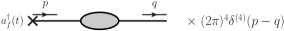
Figure 6: Green function that gives $\langle\boldsymbol{q}|a_{f}^{\dagger}(t)|0\rangle$ after application of reduction method. Since the graphical 2-point function is often treated with the momentum-conservation delta function omitted, its presence has been indicated explicitly.

It can also be checked that the same matrix element of the conjugated operator, intended to annihilate particles, is zero:

$$\langle\boldsymbol{q}|a_{f}(t)|0\rangle=0.$$ (95)

This follows from the factor $E_{\boldsymbol{q}}+q^{0}$ in the rule (93) for the vertex for $a_{f}(t)$, since with an on-shell final-state particle, $q^{0}=-E_{-\boldsymbol{q}}=-E_{\boldsymbol{q}}$.

IX.3.2 Example: Vacuum to three particles

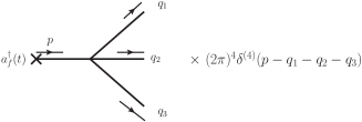
Figure 7: Lowest-order graph for $\langle\boldsymbol{q}_{1},\boldsymbol{q}_{2},\boldsymbol{q}_{3};\,{\rm out}|a_{f}^{\dagger}(t)|0\rangle$, with explicit delta-function for momentum conservation.

In $\phi^{4}$ theory with coupling $\lambda$, the lowest order graph for $a_{f}^{\dagger}(t)$ to create something other than a single particle is shown in Fig. 7, where the final state has 3 (on-shell) particles of momenta $q_{1}$, $q_{2}$, and $q_{3}$. From the Feynman rules, we get

$$\langle\boldsymbol{q}_{1},\boldsymbol{q}_{2},\boldsymbol{q}_{3};\,{\rm out}|\,a_{f}^{\dagger}(t)\,|0\rangle =\lambda\tilde{f}(\boldsymbol{q})\,\frac{E_{\boldsymbol{q}}+q^{0}}{2E_{\boldsymbol{q}}}\frac{1}{(q^{0})^{2}-\boldsymbol{q}^{2}-m^{2}+i\epsilon}\,e^{-i(E_{\boldsymbol{q}}-q^{0})t}\,+\,O(\lambda^{2})$$

$$=\lambda\tilde{f}(\boldsymbol{q})\,\frac{1}{2E_{\boldsymbol{q}}(q^{0}-E_{\boldsymbol{q}}+i\epsilon)}\,e^{-i(E_{\boldsymbol{q}}-q^{0})t}\,+\,O(\lambda^{2}).$$ (96)

Here $\boldsymbol{q}=\sum_{j=1}^{3}\boldsymbol{q}_{j}$ and $q^{0}=\sum_{j=1}^{3}E_{\boldsymbol{q}_{j}}$. Note that at the order of perturbation theory to which we are working, the mass value in the free propagator and the physical particle mass are equal: $m_{\rm phys}=m+O(\lambda)$, so here we do not need to be careful whether $m$ or $m_{\rm phys}$ is used in the calculation.

The matrix element in (IX.3.2) is non-zero. So the calculation shows unambiguously that the operator $a_{f}^{\dagger}(t)$, when applied to the vacuum, creates more than a single particle. We can quantify by how much, by computing the corresponding contribution to the squared norm of the state $a_{f}^{\dagger}(t)|0\rangle$, i.e., to $\left\|a_{f}^{\dagger}(t)|0\rangle\right\|^{2}$:

$$\frac{1}{3!}\int\mathop{\widetilde{\mathop{{\mathrm{d}}{}q_{1}}\nolimits}}\nolimits\mathop{\widetilde{\mathop{{\mathrm{d}}{}q_{2}}\nolimits}}\nolimits\mathop{\widetilde{\mathop{{\mathrm{d}}{}q_{3}}\nolimits}}\nolimits\,\left|\langle\boldsymbol{q}_{1},\boldsymbol{q}_{2},\boldsymbol{q}_{3};\,{\rm out}|\,a_{f}^{\dagger}(t)\,|0\rangle\right|^{2}={} \frac{\lambda^{2}}{3!}\int\mathop{\widetilde{\mathop{{\mathrm{d}}{}q_{1}}\nolimits}}\nolimits\mathop{\widetilde{\mathop{{\mathrm{d}}{}q_{2}}\nolimits}}\nolimits\mathop{\widetilde{\mathop{{\mathrm{d}}{}q_{3}}\nolimits}}\nolimits\,|\tilde{f}(\boldsymbol{q})|^{2}\left|\frac{E_{\boldsymbol{q}}+q^{0}}{2E_{\boldsymbol{q}}}\right|^{2}\frac{1}{\left[(q^{0})^{2}-\boldsymbol{q}^{2}-m^{2}\right]^{2}}$$ (97)

$$+\text{higher order}.$$

(The overall factor of $1/3!$ is to compensate double counting of indistinguishable states of identical particles.) This is linearly divergent in the UV. To see this, we notice that the wave function $\tilde{f}(\boldsymbol{q})$ strongly restricts the total 3-momentum $\boldsymbol{q}$ to finite values. We can integrate freely over two of the final-state momenta, say $\boldsymbol{q}_{1}$ and $\boldsymbol{q}_{2}$. When these values are large and in different directions, so is the third. Let $\Lambda$ be the order of magnitude of these momenta. Then the propagator denominator is of order $\Lambda^{2}$, and the factor $(E_{\boldsymbol{q}}+q^{0})/2E_{\boldsymbol{q}}$ is of order $\Lambda$ divided by a finite mass scale. Thus the power at large $\Lambda$ is $\Lambda^{1}$, and the integral is linearly divergent as claimed.

As we know from renormalization theory, such UV power counting corresponds to simple dimensional counting, and therefore it applies equally to higher order graphs. At best the UV divergences can be modified by renormalization-group resummation.

The fact that calculation gives an infinite norm for $a_{f}^{\dagger}(t)|0\rangle$ shows that $a_{f}^{\dagger}(t)|0\rangle$ is not in the Hilbert space of the theory. At best it can be said to be in some bigger space (not a Hilbert space), which would allow the manipulations given above to be valid. In any case it is not a physical state, and vectors in the bigger space could well have pathological properties compared with those of physical states in the Hilbert space.

Notice that the extra multiparticle contributions to the state $a_{f}^{\dagger}(t)|0\rangle$ do not disappear when a limit of infinite time is taken. This is because changing $t$ simply changes the phase in (IX.3.2) but not the magnitude, and the same applies to all higher order contributions. The contribution to the norm of the state is time-independent. Thus the limits as $t$ goes to $-\infty$ or $+\infty$ of $a_{f}^{\dagger}(t)|0\rangle$ do not exist. Such limits would be called strong limits, if they existed.

It is important that the existence of a divergence in the state is distinct from the existence of the extra multiparticle contributions. This can be seen be going to theory in a different space-time dimension. In a space-time dimension $n$ the degree of divergence of the natural generalization of (97) is $2n-7$. We get convergence if $n<3.5$. Thus in the integer dimensions 3 and 2 in which the theory is super-renormalizable, there is no UV divergence in (97), but the result remains non-zero. The existence of divergence in the physical case $n=4$ merely dramatizes the issue that the putative creation operator applied to the vacuum creates more than the intended single particle. That issue is unchanged when there is no UV divergence.

IX.3.3 Annihilation operator creates particles

Similarly, although the one-particle-to-vacuum matrix element of the would-be annihilation operator $a_{f}(t)$ is zero, the matrix elements to multi-particle states are non-zero. For example, we can calculate $\langle\boldsymbol{q}_{1},\boldsymbol{q}_{2},\boldsymbol{q}_{3};\,{\rm out}|a_{f}(t)|0\rangle$. The only differences compared with the corresponding matrix element of $a_{f}^{\dagger}(t)$ are: A change of $\tilde{f}(\boldsymbol{q})$ to its complex conjugate $\tilde{f}^{*}(\boldsymbol{q})$; a complex conjugation of the $t$-dependent phase; a replacement of $q^{0}$ by $-\sum_{j=1}^{3}E_{\boldsymbol{q}_{j}}$ and of $\boldsymbol{q}$ by $-\sum_{j=1}^{3}\boldsymbol{q}_{j}$. The result remains non-zero.

IX.3.4 Generalizations

Many more examples can readily constructed.

Similar considerations also apply if more than one $a_{f}^{\dagger}(t)$ operator is applied to the vacuum, with the intent of creating an initial state consisting of two or more particles. However, note that if more than one operator is applied, as in $a_{f_{1}}^{\dagger}(t_{2})a_{f_{2}}^{\dagger}(t_{1})|0\rangle$, the fields in the operator product $a_{f_{1}}^{\dagger}(t_{2})a_{f_{2}}^{\dagger}(t_{1})$ are simply multiplied, without a time-ordering operations. The use of standard Feynman diagram methods applies to $a_{f_{1}}^{\dagger}(t_{2})a_{f_{2}}^{\dagger}(t_{1})|0\rangle$ if $t_{2}>t_{1}$.

IX.3.5 Weak limit v. strong limit

Suppose instead of a state of three final-state particles of definite momentum, we used a normalizable state,

$$|G;{\rm out}\rangle\stackrel{{\scriptstyle\textrm{def}}}{{=}}\int\mathop{\widetilde{\mathop{{\mathrm{d}}{}q_{1}}\nolimits}}\nolimits\mathop{\widetilde{\mathop{{\mathrm{d}}{}q_{2}}\nolimits}}\nolimits\mathop{\widetilde{\mathop{{\mathrm{d}}{}q_{3}}\nolimits}}\nolimits\,|\boldsymbol{q}_{1},\boldsymbol{q}_{2},\boldsymbol{q}_{3};\,{\rm out}\rangle\,\tilde{G}(\boldsymbol{q}_{1},\boldsymbol{q}_{2},\boldsymbol{q}_{3}).$$ (98)

Then Eq. (IX.3.2) would be replaced by

$$\langle G;\,{\rm out}|\,a_{f}^{\dagger}(t)\,|0\rangle=\lambda\int\mathop{\widetilde{\mathop{{\mathrm{d}}{}q_{1}}\nolimits}}\nolimits\mathop{\widetilde{\mathop{{\mathrm{d}}{}q_{2}}\nolimits}}\nolimits\mathop{\widetilde{\mathop{{\mathrm{d}}{}q_{3}}\nolimits}}\nolimits\,\tilde{G}^{*}(\boldsymbol{q}_{1},\boldsymbol{q}_{2},\boldsymbol{q}_{3})\times\\ \times\tilde{f}(\boldsymbol{q})\,\frac{1}{2E_{\boldsymbol{q}}(q^{0}-E_{\boldsymbol{q}}+i\epsilon)}\,e^{-i(E_{\boldsymbol{q}}-q^{0})t}\,+\,O(\lambda^{2}),$$ (99)

still with $\boldsymbol{q}=\sum_{j=1}^{3}\boldsymbol{q}_{j}$ and $q^{0}=\sum_{j=1}^{3}E_{\boldsymbol{q}_{j}}$. The oscillations in the integrand imply that when $t\to-\infty$ with $G$ fixed, the matrix element rapidly goes to zero. This is an example of the property that $a_{f}^{\dagger}(t)$ converges weakly to a creation operator of a single particle. But we have already seen that the strong limit, i.e., the limit of the state $a_{f}^{\dagger}(t)|0\rangle$, does not exist.

With a normalizable state instead of particles of definite momenta, how negative $t$ needs to be for the matrix element to be close to the asymptote depends on the wave functions $\tilde{G}$ and $\tilde{f}$.

As a physical illustration, suppose $\tilde{G}$ is real, positive, and tightly peaked around a particular momentum for each particle. Then by the results of Sec. VII, it corresponds to a state of three particles of almost definite momenta that are localized quite close to the origin of spatial coordinates at time $t=0$. (We could even insert a $\boldsymbol{q}_{j}$-dependent phase to separate the particles a bit.) We also choose the wave function in $a_{f}^{\dagger}$ to be similarly localized.

For this case, the matrix element (99) rapidly decreases to zero as $t$ is moved away from zero time.

Now change the wave function by a phase as follows:

$$\tilde{G}(\boldsymbol{q}_{1},\boldsymbol{q}_{2},\boldsymbol{q}_{3})\mapsto\tilde{G}(\boldsymbol{q}_{1},\boldsymbol{q}_{2},\boldsymbol{q}_{3})\,e^{-i(E_{\boldsymbol{q}}-q^{0})t_{1}},$$ (100)

with $t_{1}$ being some very large negative value. This corresponds to a state that at time $t_{1}$ has the three particles spatially localized to the same region as where the wave function $f(t_{1},\boldsymbol{x})$ is localized at the same time.

At $t=0$ the matrix element in (99) is very small because of the rapid oscillations in the integrand that are now in the wave function. However, when the time in the intended creation operator is set to $t_{1}$, i.e., $t=t_{1}$, the oscillations are canceled, and we get a large value. It is only when $t$ is significantly more negative than $t_{1}$ that the limiting behavior for a creation of an one-particle initial state is approached.

Since $t_{1}$ is arbitrary, we cannot provide a single time below which the state $a_{f}^{\dagger}(t)|0\rangle$ itself is close to zero. We have thus seen the non-existence of the strong limit with calculations that only use normalizable states. Obviously the calculation with particles of definite momenta shows the same result more simply. But the analysis with normalizable states works purely within the Hilbert space of states and lends itself to physical interpretation.

IX.3.6 Remarks

(a)	(b)

Figure 8: (a) Illustrating trajectories and hence spatial location of state components with extra particles that are created by $a_{f}^{\dagger}(t)$ when $|t|$ is large and negative. (b) The trajectories of the single particle corresponding to the intended single-particle state component created by the same operator. In both cases, the dot indicates where the particle(s) were created.

The line of argument just given shows that even though the operator $a_{f}^{\dagger}(t)$ creates a lot of extra particles, they are asymptotically in a different region of space time than the intended single particle. More explicitly, observe that the coordinate-space wave function $f(x)$ is concentrated near the classical trajectory of the particle. When $t\to-\infty$, its position is infinitely far away from the origin. Now, for graphs with multi-particle final states, the propagator attached to the vertex for $a_{f}^{\dagger}(t)$ is never close to its pole. Thus the invariant distances involved between the ends of the propagator are of order $1/m$ or smaller. Hence when $t\to-\infty$, the production region of the particles is infinitely far away, as illustrated in Fig. 8. Thus they essentially all avoid hitting a finite sized detector surrounding the intended collision region in a scattering experiment. This is a fairly physical reason why the large extra contributions to the initial state created by $a_{f}^{\dagger}(t)$ do not contribute in the LSZ proof to calculations of the S-matrix itself, despite the delicate mathematical grounding caused by the UV divergence in the state vector.

A more abstract mathematical way of analyzing this situation is to observe that as $t\to\pm\infty$, the phase factors in Eqs. (92) and (93) oscillate infinitely rapidly except when the momentum $p$ or $q$ corresponds to the intended single-particle state. If the vertices appear inside a quantity that has a suitable integral over momentum, then the infinitely rapid oscillations cause a corresponding vanishing of the corresponding contribution in the integral. The oscillations mathematically implement the physical statement that the extra particles created or destroyed by the operators are infinitely far from the scattering region.

However, we may not always want to use a limit of infinite time. Notably, if we wish to calculate scattering with an initial particle that is unstable (but perhaps long lived), then it is natural to use an operator like $a_{f}^{\dagger}(t)$ to create the particle at a finite time that corresponds to the experimental source of the particle. Then the extra particles created by $a_{f}^{\dagger}(t)$ can easily be in an experimentally accessible location.

IX.4 General analysis of divergence from spectral representation

The UV divergence in $\|a_{f}^{\dagger}(t)|0\rangle\|^{2}$ was found in an illustrative calculation in Sec. IX.3 with the use of the reduction formula. We will now obtain a general result for this quantity from the spectral representation, whose properties were summarized in Sec. VI. From the representation Eq. (VI) for the 2-field correlator, and the definition (90a) of $a_{f}^{\dagger}(t)$, it follows that

$$\|a_{f}^{\dagger}(t)|0\rangle\|^{2}={} \langle 0|a_{f}(t)a_{f}^{\dagger}(t)|0\rangle$$

$$={} \int_{0}^{\infty}\mathop{{\mathrm{d}}{}s}\nolimits\rho(s)\int\mathop{\widetilde{\mathop{{\mathrm{d}}{}p}\nolimits}}\nolimits\mathop{\widetilde{\mathop{{\mathrm{d}}{}q}\nolimits}}\nolimits\int\frac{\mathop{{\mathrm{d}}^{3}{}\boldsymbol{k}}\nolimits}{(2\pi)^{3}2\sqrt{\boldsymbol{k}+s}}\tilde{f}(\boldsymbol{p})^{*}\tilde{f}(\boldsymbol{q})\int\mathop{{\mathrm{d}}^{3}{}\boldsymbol{x}}\nolimits\mathop{{\mathrm{d}}^{3}{}\boldsymbol{y}}\nolimits$$

$$\left[e^{iE_{\boldsymbol{p}}x^{0}-i\boldsymbol{p}\cdot\boldsymbol{x}}\overleftrightarrow{\frac{\partial}{\partial x^{0}}}e^{-i\sqrt{\boldsymbol{k}+s}x^{0}+i\boldsymbol{k}\cdot\boldsymbol{x}}\right]\left[e^{-iE_{\boldsymbol{q}}y^{0}+i\boldsymbol{q}\cdot\boldsymbol{x}}\overleftrightarrow{\frac{\partial}{\partial y^{0}}}e^{i\sqrt{\boldsymbol{k}+s}y^{0}-i\boldsymbol{k}\cdot\boldsymbol{y}}\right],$$ (101)

with $x^{0}$ and $y^{0}$ being set to $t$ after the derivatives are taken. Straightforward manipulations lead to

$$\|a_{f}^{\dagger}(t)|0\rangle\|^{2}={} \int\mathop{\widetilde{\mathop{{\mathrm{d}}{}p}\nolimits}}\nolimits|\tilde{f}(\boldsymbol{p})|^{2}\int_{0}^{\infty}\mathop{{\mathrm{d}}{}s}\nolimits\rho(s)\frac{\left(\sqrt{\boldsymbol{p}^{2}+s}+\sqrt{\boldsymbol{p}^{2}+m_{\rm phys}^{2}}\right)^{2}}{4\sqrt{\boldsymbol{p}^{2}+s}\,\sqrt{\boldsymbol{p}^{2}+m_{\rm phys}^{2}}}.$$ (102)

Now the spectral function can be found calculationally from analyzing the propagator and self-energy graphs. At large $p^{2}$, the propagator $\hat{G}_{2}(p^{2})$ is known to behave like $1/p^{2}$ times logarithms, order-by-order in perturbation theory. Hence from the spectral representation (56) for $\hat{G}_{2}(p^{2})$, the spectral function $\rho(s)$ behaves like $1/s$ times logarithms.

In Eq. (102), the wave function limits $\boldsymbol{p}$ to finite values, while at large $s$ the last factor grows like $\sqrt{s}$. It follows that order-by-order in perturbation theory, $\|a_{f}^{\dagger}(t)|0\rangle\|^{2}$ has the same kind of power divergence that we found in an explicit calculation. The state’s norm can only be finite if the true non-perturbative $\rho(s)$ falls sufficiently more rapidly than $1/s^{3/2}$.

The operator $a_{f}^{\dagger}(t)$ was defined by an integral over the field and its time derivative at fixed time. Therefore the UV divergence in $\|a_{f}^{\dagger}(t)|0\rangle\|^{2}$ shows that there is a failure of localization on a quantization surface of fixed time. The presence or absence of the divergence depends on the dynamics of the theory. Localization does work in a theory that is sufficiently convergent in the UV, e.g., in a free-field theory, or in a sufficiently super-renormalizable theory. The culprit is not the field itself, but its time derivative. The time derivative gives two factors of $q^{0}$ in the integrand in (97), and without those factors the integral would be convergent. See Ref. [32] for a further examination of the localization properties of fields on a quantization surface, in the free-field case, and for an examination of interesting differences between equal-time and light-front quantization.

In a theory where there is no UV divergence in $a_{f}^{\dagger}(t)|0\rangle$, Eq. (102) nonperturbatively quantifies the multi-particle contribution to the state.

IX.5 Modified creation and annihilation operators

What allowed the operators $a_{f}^{\dagger}(t)$ and $a_{f}(t)$ to create and annihilate states other than the intended single-particle states was the use of the field operator at fixed time. This gave an integral over all energy in the momentum-space version, as exhibited in the Feynman rules (92) and (93).

A simple way to enforce the single-particle condition is to restrict the energy explicitly. Let us implement this by smoothly averaging over a range $\Delta t$ of time with an averaging function $F(t^{\prime}-t,\Delta t)$, and then taking $\Delta t$ to infinity. We define the averaged operator by

$$A_{f}^{\dagger}(t;\Delta t) \stackrel{{\scriptstyle\textrm{def}}}{{=}}\frac{1}{c^{*}}\int\mathop{{\mathrm{d}}{}t^{\prime}}\nolimits F(t^{\prime}-t,\Delta t)\,a_{f}^{\dagger}(t^{\prime}).$$ (103)

The averaging function is required to be real, non-negative, and to integrate to unity:

$$\int\mathop{{\mathrm{d}}{}t^{\prime}}\nolimits F(t^{\prime}-t,\Delta t)=1.$$ (104)

In the definition (103), the factor $1/c^{*}$ is to normalize $A_{f}^{\dagger}(t;\Delta t)$ so that, as we will see, the one-particle state that it creates has the standard normalization. A suitable averaging function is a Gaussian:

$$F(t^{\prime}-t,\Delta t)=\frac{e^{-(t^{\prime}-t)^{2}/(\Delta t)^{2}}}{\sqrt{\pi}\Delta t}.$$ (105)

A number of alternative forms may be written for the operator $A_{f}^{\dagger}(t;\Delta t)$. Let ${x^{\prime}}^{\mu}=(t^{\prime},\boldsymbol{x}^{\prime})$. Then

$$A_{f}^{\dagger}(t;\Delta t) =\frac{-i}{c^{*}}\int\mathop{{\mathrm{d}}^{4}{}x^{\prime}}\nolimits F(t^{\prime}-t,\Delta t)\left[f(x^{\prime})\overleftrightarrow{\frac{\partial}{\partial t^{\prime}}}\phi(x^{\prime})\right]$$

$$=\frac{i}{c^{*}}\int\mathop{{\mathrm{d}}^{4}{}x^{\prime}}\nolimits\phi(x^{\prime})\left[\frac{\partial F(t^{\prime}-t,\Delta t)}{\partial t^{\prime}}f(x^{\prime})+2F(t^{\prime}-t,\Delta t)\frac{\partial f(x^{\prime})}{\partial t^{\prime}}\right]$$

$$=\frac{1}{c^{*}}\int\frac{\mathop{{\mathrm{d}}^{4}{}p}\nolimits}{(2\pi)^{4}}\tilde{\phi}(p)\,\tilde{f}(\boldsymbol{p})\,\frac{E_{\boldsymbol{p}}+p^{0}}{2E_{\boldsymbol{p}}}\,e^{-i(E_{\boldsymbol{p}}-p^{0})t}\,\tilde{F}(p^{0}-E_{\boldsymbol{p}},\Delta t).$$ (106)

In the second line, $A_{f}^{\dagger}(t;\Delta t)$ is written as a simple integral of the field with a function. It is probably best to treat that second line as the actual definition of $A_{f}^{\dagger}(t;\Delta t)$, since it avoids any difficulties about localization of fields on a quantization surface. The previous manipulations can then be regarded as simply motivational, to indicate why that particular formula is used. Our earlier results showing that the operators $a_{f}^{\dagger}(t)$ fail to exist as operators on the space of physical normalizable states show that the steps leading to the second line of Eq. (IX.5) are on dangerous mathematical ground.

In the last line we used the Fourier transform of the field,

$$\phi(x)=\int\frac{\mathop{{\mathrm{d}}^{4}{}p}\nolimits}{(2\pi)^{4}}\tilde{\phi}(p)\,e^{ip\cdot x},$$ (107)

to write a momentum-space expression, with the Fourier transform of $F$ defined by

$$\tilde{F}(\delta E,\Delta t)=\int\mathop{{\mathrm{d}}{}t^{\prime}}\nolimits e^{i\delta E(t^{\prime}-t)}F(t^{\prime}-t,\Delta t).$$ (108)

In the case of the Gaussian, the Fourier-transformed averaging function is

$$\tilde{F}(\delta E,\Delta t)=e^{-\delta E^{2}\Delta t^{2}/4}.\quad\text{({\hbox{F}} Gaussian)}$$ (109)

From the last line of Eq. (IX.5) follows the Feynman rule for the vertex corresponding to the operator $A_{f}^{\dagger}(t;\Delta t)$. It is a simple generalization of (92), containing an extra factor $\tilde{F}(p^{0}-E_{\boldsymbol{p}},\Delta t)$:

$$\text{Vertex}(A_{f}^{\dagger}(t;\Delta t))=\int\frac{\mathop{{\mathrm{d}}^{4}{}p}\nolimits}{(2\pi)^{4}}\tilde{f}(\boldsymbol{p})\,\frac{E_{\boldsymbol{p}}+p^{0}}{2E_{\boldsymbol{p}}}\,e^{-i(E_{\boldsymbol{p}}-p^{0})t}\,\tilde{F}(p^{0}-E_{\boldsymbol{p}},\Delta t).$$ (110)

It is the new factor $\tilde{F}$ that enforces the restriction that in the $\Delta t\to\infty$ limit, $A_{f}^{\dagger}(t;\Delta t)$ creates a single particle and nothing else. That is, when we take the limit of infinite averaging time, $\Delta t\to\infty$, $\tilde{F}$ goes to zero unless $\delta E=0$, i.e., unless the on-shell condition $p^{0}=E_{\boldsymbol{p}}$ is obeyed.

Formulas for the conjugate operator $A_{f}(t;\Delta t)$ are:

$$A_{f}(t;\Delta t) =\frac{-i}{c}\int\mathop{{\mathrm{d}}^{4}{}x^{\prime}}\nolimits\phi(x^{\prime})\left[\frac{\partial F(t^{\prime}-t,\Delta t)}{\partial t^{\prime}}f^{*}(x^{\prime})+2F(t^{\prime}-t,\Delta t)\frac{\partial f^{*}(x^{\prime})}{\partial t^{\prime}}\right]$$

$$=\frac{1}{c}\int\frac{\mathop{{\mathrm{d}}^{4}{}p}\nolimits}{(2\pi)^{4}}\tilde{\phi}(-p)\,\tilde{f}^{*}(\boldsymbol{p})\,\frac{E_{\boldsymbol{p}}+p^{0}}{2E_{\boldsymbol{p}}}\,e^{i(E_{\boldsymbol{p}}-p^{0})t}\,\tilde{F}^{*}(p^{0}-E_{\boldsymbol{p}},\Delta t),$$ (111)

and the corresponding vertex is

$$\text{Vertex}(A_{f}(t;\Delta t))=\int\frac{\mathop{{\mathrm{d}}^{4}{}q}\nolimits}{(2\pi)^{4}}\tilde{f}^{*}(\boldsymbol{q})\,\frac{E_{\boldsymbol{q}}+q^{0}}{2E_{\boldsymbol{q}}}\,e^{i(E_{\boldsymbol{q}}-q^{0})t}\,\tilde{F}^{*}(q^{0}-E_{\boldsymbol{q}},\Delta t).$$ (112)

When these formulas are used in calculations, it should be remembered that for the $A_{f}^{\dagger}$ vertex the momentum $p$ flows into the rest of the graph from $A_{f}^{\dagger}$ vertex, whereas the opposite is true for the momentum $q$ at the $A_{f}$ vertex, as explained after Eq. (93).

Furthermore, a Green function is defined using a time-ordered product of fields. So except in asymptotic situations, e.g., in matrix elements with in- and out-states, there is a mismatch between a Green function with the vertex implied by Eq. (IX.5) and an actual matrix element of the operator.

Finally, we need operators that create and destroy particles in the in- and out-states, as the relevant limits. The creation operators are defined as

$$A_{f;\,{\rm in}}^{\dagger} \stackrel{{\scriptstyle\textrm{def}}}{{=}}\lim_{\begin{subarray}{c}t\to-\infty\\ \Delta t\to\infty\\ \Delta t/|t|\to 0\end{subarray}}A_{f}^{\dagger}(t;\Delta t),$$ (113)

$$A_{f;\,{\rm out}}^{\dagger} \stackrel{{\scriptstyle\textrm{def}}}{{=}}\lim_{\begin{subarray}{c}t\to+\infty\\ \Delta t\to\infty\\ \Delta t/|t|\to 0\end{subarray}}A_{f}^{\dagger}(t;\Delta t),$$ (114)

with the annihilation operators defined as the hermitian conjugates. The limit $\Delta t\to\infty$ ensures that the created and destroyed particles are just the intended single particles, because of the factor $\tilde{F}(p^{0}-E_{\boldsymbol{p}},\Delta t)$ in the vertex for $A_{f}^{\dagger}(t;\Delta t)$. The limit $t\to\pm\infty$ is needed to correspond to the application to the asymptotics of scattering processes, as usual. To ensure that the range of time involved in creating or destroying incoming and outgoing particles is much less than the time between the region of scattering and the creation and destruction of asymptotic particles, we require that in the infinite-time limits $t$ and $\Delta t$ are taken such that $\Delta t/|t|\to 0$.

These time scales correspond to experimental reality, where the times involved are short of achieved the strict mathematical limits.

The definitions (113) and (114) are as strong limits. Given the known result that the corresponding definitions for the elementary creation operators $a_{f}^{\dagger}(t)$ are only weak limits, it is important to verify explicitly that the strong limits exist.

Having defined the operators $A_{f}^{\dagger}(t;\Delta t)$ and $A_{f}(t;\Delta t)$, and their limits as $t\to\pm\infty$, it is necessary to verify that they have the properties that their definitions were intended to have and that they do not have the deficiencies illustrated in Sec. IX.3 for the LSZ versions of the operators. To avoid a circularity of the logic, we will postpone this analysis until after the proof of the reduction formula is completed. The results are found in Sec. XII below.

X Simple matrix elements of annihilation and creation operators

In this section we obtain some of the most basic properties of the annihilation and creation operators. These involve the action of one operator on the vacuum or the vacuum expectation value of a product of two operators. These can be analyzed simply and non-perturbatively in the exact theory with the aid of the spectral representation; the analysis does not need the reduction formula. Not only are the results of interest in their own right, but they will be useful ingredients for work in later sections.

X.1 One operator on vacuum

From the vertex formula (110) and translation invariance of $\langle 0|\phi(x)|0\rangle$, it follows that the vacuum expectation value of one operator is

$$\langle 0|A_{f}^{\dagger}(t;\Delta t)|0\rangle=\frac{1}{2c^{*}}\langle 0|\phi(0)|0\rangle\tilde{f}(\boldsymbol{0})\,e^{-im_{\rm phys}t}\,\tilde{F}(-m_{\rm phys},\Delta t).$$ (115)

This goes to zero as $\Delta t\to\infty$, because $\tilde{F}(-m_{\rm phys})$ does, and this happens independently of $t$. In particular, we can take $t$ to $\pm\infty$ more rapidly than $\Delta t$, as is needed for the in- and out-operators. Thus

$$\lim_{\Delta t\to\infty}\langle 0|A_{f}^{\dagger}(t;\Delta t)|0\rangle=\langle 0|A_{f;\,{\rm in}}^{\dagger}|0\rangle=\langle 0|A_{f;\,{\rm out}}^{\dagger}|0\rangle=0.$$ (116)

From the vertex formula (110) and the known one-particle-to-vacuum matrix element of $\langle\boldsymbol{p}|\phi(x)|0\rangle$ it follows that the $A_{f}^{\dagger}$ operators have the desired one-particle-to-vacuum matrix elements, independently of $t$ and $\Delta t$. Hence

$$\langle\boldsymbol{p}|A_{f}^{\dagger}(t;\Delta t)|0\rangle=\langle\boldsymbol{p}|A_{f;\,{\rm in}}^{\dagger}|0\rangle=\langle\boldsymbol{p}|A_{f;\,{\rm out}}^{\dagger}|0\rangle=\tilde{f}(\boldsymbol{p}).$$ (117)

Similar we have the following matrix elements of an annihilation operator with a normalizable one-particle state:

$$\langle 0|A_{f}(t;\Delta t)|g\rangle=\langle 0|A_{f;\,{\rm in}}|g\rangle=\langle 0|A_{f;\,{\rm out}}|g\rangle=\int\mathop{\widetilde{\mathop{{\mathrm{d}}{}p}\nolimits}}\nolimits\tilde{f}^{*}(\boldsymbol{p})\tilde{g}(\boldsymbol{p}).$$ (118)

Matrix elements of a creation operator between a multi-particle state and the vacuum vanish in the $\Delta t\to\infty$ limit. To see this, we follow the pattern used in the example calculations, with basis momentum states:

$$\langle\boldsymbol{q}_{1},\dots,\boldsymbol{q}_{n};\,{\rm in}|\,A_{f}^{\dagger}(t;\Delta t)\,|0\rangle=(\mbox{time-independent})\,e^{-i(E_{\boldsymbol{q}}-q^{0})t}\,\tilde{F}(q^{0}-E_{\boldsymbol{q}},\Delta t),$$ (119)

where $q^{0}$ and $\boldsymbol{q}$ are the total energy and 3-momentum of the $n$-particle state. As $\Delta t\to\infty$, this vanishes, because the $\tilde{F}$ factor vanishes. We now wish to show that the strong limit of the state $A_{f}^{\dagger}(t;\Delta t)|0\rangle$ as $\Delta t\to\infty$ is the single-particle state $|f\rangle$. From the already-calculated one-particle component in $A_{f}^{\dagger}(t;\Delta t)|0\rangle$ it follows that the size of the rest of the state is given by

$$\left\|A_{f}^{\dagger}(t;\Delta t)|0\rangle-|f\rangle\right\|^{2}=\operatorname*{\mathchoice{\ooalign{$\displaystyle\sum$\cr$\displaystyle\int$\cr}}{\ooalign{\raisebox{0.14pt}{\scalebox{0.7}{$\textstyle\sum$}}\cr$\textstyle\int$\cr}}{\ooalign{\raisebox{0.2pt}{\scalebox{0.6}{$\scriptstyle\sum$}}\cr$\scriptstyle\int$\cr}}{\ooalign{\raisebox{0.2pt}{\scalebox{0.6}{$\scriptstyle\sum$}}\cr$\scriptstyle\int$\cr}}}_{\begin{subarray}{c}\rm except\\ \rm single\\ \rm particle\end{subarray}}\!\!\mathop{{\mathrm{d}}{}X}\nolimits\left|\langle X;\,{\rm out}|A_{f}^{\dagger}(t;\Delta t)|0\rangle\right|^{2}=(\mbox{time-independent})\times\,\left|\tilde{F}(q^{0}-E_{\boldsymbol{q}},\Delta t)\right|^{2},$$ (120)

where the integral over $X$ is a sum and integral over basis states for all but the single-particle states. The desired strong limit follows, plus a result for $\Delta t\to\infty$ independently of $t$:

$$\lim_{\Delta t\to\infty}A_{f}^{\dagger}(t;\Delta t)|0\rangle=A^{\dagger}_{f;\,{\rm in}}|0\rangle=A^{\dagger}_{f;\,{\rm out}}|0\rangle=|f\rangle.$$ (121)

Here, as usual $|f\rangle=|f;\,{\rm in}\rangle=|f;\,{\rm out}\rangle=\int\mathop{\widetilde{\mathop{{\mathrm{d}}{}p}\nolimits}}\nolimits\,|\boldsymbol{p}\rangle\,\tilde{f}(\boldsymbol{p})$.

In textbooks it is very common to use the interaction picture, and to employ three kinds of basis state: a free basis, and in-basis, and an out-basis. Therefore it is necessary to emphasize that in (121) and elsewhere in this paper, the basis states are strictly in the in- or out-basis, unless specifically indicated otherwise. Haag’s theorem guarantees that the state space spanned by the in- and out-bases in an interacting theory is orthogonal to the corresponding state space of the free theory.

Very similarly, we find that the operator $\lim_{\Delta t\to\infty}A_{f}(t;\Delta t)$ annihilates the vacuum:

$$\lim_{\Delta t\to\infty}A_{f}(t;\Delta t)|0\rangle=0,$$ (122)

and equally for the in- and out-versions of the annihilation operators.

None of the results above should be a surprise. The definition of $A_{f}^{\dagger}$ was specifically designed to make them valid. Nevertheless, it is useful to show directly from the definitions that in the most elementary cases the properties are valid.

X.2 Vacuum matrix elements of two operators

Consider now the vacuum expectation value of the product of two $A^{\dagger}_{f}(t,\Delta t)$ operators: $\langle 0|A_{g}^{\dagger}(t_{2};\Delta t_{2})A_{g}^{\dagger}(t_{1};\Delta t_{1})|0\rangle$. In view of later uses of results from this section, we will start with independently chosen values of the parameters $t_{j}$ and $\Delta t_{j}$. From the definition (IX.5) of the operators and the spectral representation (VI), standard manipulations give

$$\langle 0|A_{f}^{\dagger}(t_{2};\Delta t_{2})A_{g}^{\dagger}(t_{1};\Delta t_{1})|0\rangle={} \frac{1}{{c^{*}}^{2}}\int\frac{\mathop{{\mathrm{d}}^{4}{}p}\nolimits}{(2\pi)^{3}}\rho(p^{2})\theta(p^{0})\,\tilde{g}(-\boldsymbol{p})\,\tilde{f}(\boldsymbol{p})\,\frac{E_{-\boldsymbol{p}}-p^{0}}{2E_{-\boldsymbol{p}}}\,\frac{E_{\boldsymbol{p}}+p^{0}}{2E_{\boldsymbol{p}}}\times$$

$$\hskip 19.91692pt\times\,e^{-i(E_{-\boldsymbol{p}}+p^{0})t_{2}}\,e^{-i(E_{\boldsymbol{p}}-p^{0})t_{1}}\,\tilde{F}(-p^{0}-E_{-\boldsymbol{p}},\Delta t_{2})\,\tilde{F}(p^{0}-E_{\boldsymbol{p}},\Delta t_{1})$$

$$={} \frac{1}{{c^{*}}^{2}}\int\frac{\mathop{{\mathrm{d}}^{4}{}p}\nolimits}{(2\pi)^{3}}\rho(p^{2})\theta(p^{0})\,\tilde{g}(-\boldsymbol{p})\,\tilde{f}(\boldsymbol{p})\,\frac{p^{2}-m_{\rm phys}^{2}}{4E_{\boldsymbol{p}}^{2}}\times$$

$$\hskip 19.91692pt\times\,e^{-i(E_{\boldsymbol{p}}+p^{0})t_{2}}\,e^{-i(E_{\boldsymbol{p}}-p^{0})t_{1}}\,\tilde{F}(-p^{0}-E_{\boldsymbol{p}},\Delta t_{2})\,\tilde{F}(p^{0}-E_{\boldsymbol{p}},\Delta t_{1})$$ (123)

In a limit that $\Delta t_{2}\to\infty$, the first $\tilde{F}$ factor vanishes, since $p^{0}$ is always positive. Hence

$$\lim_{\Delta t_{2}\to\infty}\langle 0|A_{g}^{\dagger}(t_{2};\Delta t_{2})A_{f}^{\dagger}(t_{1};\Delta t_{1})|0\rangle=0,$$ (124)

independently of whether any of the other parameters ($t_{j}$, $\Delta t_{1}$) are held fixed or are taken to infinity. Hence.

$$\langle 0|A_{g;\,{\rm in}}^{\dagger}A_{f;\,{\rm in}}^{\dagger}|0\rangle=\langle 0|A_{g;\,{\rm out}}^{\dagger}A_{f;\,{\rm out}}^{\dagger}|0\rangle=0.$$ (125)

Note the lack of time dependence in (124), which is specific to the case where the vacuum expectation value is of two operators (or fewer).

The case of one creation and one annihilation operator is nonzero:

$$\langle 0|A_{g}(t_{2};\Delta t_{2})A_{f}^{\dagger}(t_{1};\Delta t_{1})|0\rangle\\ =\frac{1}{|c|^{2}}\int\frac{\mathop{{\mathrm{d}}^{4}{}p}\nolimits}{(2\pi)^{3}}\rho(p^{2})\theta(p^{0})\,\tilde{g}^{*}(\boldsymbol{p})\,\tilde{f}(\boldsymbol{p})\,\left(\frac{E_{\boldsymbol{p}}+p^{0}}{2E_{\boldsymbol{p}}}\right)^{2}\,\,e^{i(E_{\boldsymbol{p}}-p^{0})(t_{2}-t_{1})}\,\tilde{F}^{*}(p^{0}-E_{\boldsymbol{p}},\Delta t_{2})\,\tilde{F}(p^{0}-E_{\boldsymbol{p}},\Delta t_{1}).$$ (126)

When one or both $\Delta t_{j}\to\infty$, the $\tilde{F}$ factors give zero for the continuum contribution from $\rho(p^{2})$, i.e., from $p^{2}>m_{\rm phys}^{2}$, and leave only the contribution from the single particle intermediate state, with its delta-function in $\rho(p^{2})$. This is again independent of what is done with $t_{j}$. So

$$\lim_{\begin{subarray}{c}\Delta t_{1}\\ {\rm and/or}\\ \Delta t_{2}\to\infty\end{subarray}}\langle 0|A_{g}(t_{2};\Delta t_{2})A_{f}^{\dagger}(t_{1};\Delta t_{1})|0\rangle=\int\mathop{\widetilde{\mathop{{\mathrm{d}}{}p}\nolimits}}\nolimits\,\tilde{g}^{*}(\boldsymbol{p})\,\tilde{f}(\boldsymbol{p}),$$ (127)

which is the same time-independent formula as in the free theory. The result is saturated by one-particle states between the two operators. Exchanging the two operators gives zero:

$$\lim_{\begin{subarray}{c}\Delta t_{1}\\ {\rm and/or}\\ \Delta t_{2}\to\infty\end{subarray}}\langle 0|A_{f}^{\dagger}(t_{1};\Delta t_{1})A_{g}(t_{2};\Delta t_{2})|0\rangle=0,$$ (128)

and hence the commutator’s vacuum-expectation value is the standard one

$$\lim_{\begin{subarray}{c}\Delta t_{1}\\ {\rm and/or}\\ \Delta t_{2}\to\infty\end{subarray}}\langle 0|\,\left[A_{g}(t_{2};\Delta t_{2}),A_{f}^{\dagger}(t_{1};\Delta t_{1})\right]\,|0\rangle=\int\mathop{\widetilde{\mathop{{\mathrm{d}}{}p}\nolimits}}\nolimits\,\tilde{g}^{*}(\boldsymbol{p})\,\tilde{f}(\boldsymbol{p}).$$ (129)

This implies the same equations for the in and out versions of these operators. They are then compatible with the standard commutation relations for the in-operators, i.e.,

$$\left[A_{g;\,{\rm in}}^{\dagger},A_{f;\,{\rm in}}^{\dagger}\right]=\left[A_{g;\,{\rm in}},A_{f;\,{\rm in}}\right]=0,\qquad\left[A_{g;\,{\rm in}},A_{f;\,{\rm in}}^{\dagger}\right]=\int\mathop{\widetilde{\mathop{{\mathrm{d}}{}p}\nolimits}}\nolimits\,\tilde{g}^{*}(\boldsymbol{p})\,\tilde{f}(\boldsymbol{p}),$$ (130)

and the same for the out-operators. But an actual proof needs more techniques than just the spectral representation, and will have to wait until we derive the reduction formula.

XI Derivation of reduction formula

In this section, we find how to express $\langle g_{1},\dots,g_{n};\,{\rm out}|f_{1},\dots,f_{n^{\prime}};\,{\rm in}\rangle$ in terms of momentum-space Green functions and thence derive the reduction formula for the S-matrix. To make a simplification in the notation and the analysis of connected components, we restrict to the standard experimentally relevant situation of two incoming particles, i.e., $n^{\prime}=2$. The generalization to other values of $n^{\prime}$ is elementary.

The overall starting point consists of the assertions that we have a relativistic QFT obeying standard properties, that the Green functions exist, and that the full propagator has a pole at a nonzero mass. We also assume that the momentum-space Green functions have the analyticity properties attributed to them on the basis of Feynman perturbation theory. All of these properties primarily concern the off-shell Green functions.

We will use the operators defined in Sec. IX.5 for creating in- and out-states of specified particle content.

The derivation of the reduction formula has the following steps:

1. Given a particular set of momentum-space wave functions $f_{1},\dots$, define a corresponding “in state” by applying the relevant product of $A_{f;\,{\rm in}}^{\dagger}$ operators to the vacuum, thereby constructing a state with a specified momentum content in the far past. Similarly, construct an out state with the specified content in the far future. The gives a construction of the states used in $\langle g_{1},\dots,g_{n};\,{\rm out}|f_{1},f_{2};\,{\rm in}\rangle$. The aim of the following manipulations is to obtain a useful formula for the S-matrix, which appears on the right-hand side of Eq. (39).

2. Apply the definitions of the $A_{f;\,{\rm in}}^{\dagger}$ and $A_{f;\,{\rm out}}^{\dagger}$ operators. The result is a limit of the vacuum-expectation value of a product of field operators integrated over space-time, multiplied by wave functions and averaging functions.

3. Show that in the relevant infinite-time limit, the product of field operators can be replaced by a time-ordered product, i.e., an ordinary Green function.

4. By Fourier transformation, express the result in terms of the momentum-space Green functions.

5. Show that in the specified limits of infinite time, the result is of the usual form of momentum-space wave functions integrated with a quantity $S_{\boldsymbol{q}_{1},\dots,\boldsymbol{q}_{n};\,\boldsymbol{p}_{1},\boldsymbol{p}_{2}}$, as on the right-hand side of Eq. (39), and that $S_{\boldsymbol{q}_{1},\dots,\boldsymbol{q}_{n};\,\boldsymbol{p}_{1},\boldsymbol{p}_{2}}$ has the form given in the reduction formula, (75) or (76), for the connected term and related formulas for disconnected terms.

The first two steps are simply an application of our defined creation and annihilation operators, with the use of the assertion that the limits involved in their definition are strong limits. The remaining steps consist of essentially mechanical steps to calculate the inner product in terms of momentum-space Green functions, and hence in terms of quantities accessible to Feynman-graph calculations. They also verify that the inner product has the expected structure that corresponds to the existence of an S-matrix.

In addition, we will verify some properties of the states and operators that are needed to show that the expected properties used in scattering theory actually do hold.

XI.1 Construction of asymptotic states and inner product of in and out states

We have defined operators $A_{f;\,{\rm in}}^{\dagger}$ and $A_{f;\,{\rm out}}^{\dagger}$ that are intended to create asymptotic particles when applied to the vacuum. For the in-state we therefore define a generic in-state by

$$|f_{1},\dots,f_{n^{\prime}};\,{\rm in}\rangle\stackrel{{\scriptstyle\textrm{def}}}{{=}}A_{f_{1};\,{\rm in}}^{\dagger}\,\dots\,A_{f_{n^{\prime}};\,{\rm in}}^{\dagger}\,|0\rangle=\prod_{j=1}^{n^{\prime}}A_{f_{j};\,{\rm in}}^{\dagger}\,|0\rangle.$$ (131)

For each wave function, define the following quantity

$$\hat{f}_{j}(x_{j};t_{j,-},\Delta t_{j,-})=\frac{\partial F(x_{j}^{0}-t_{j,-},\Delta t_{j,-})}{\partial x_{j}^{0}}f(x_{j})+2F(x_{j}^{0}-t_{j,-},\Delta t_{j,-})\frac{\partial f(x_{j})}{\partial x_{j}^{0}}.$$ (132)

With modified variable names, this is the combination of wave function and averaging functions that appears in the second line of Eq. (IX.5) which gives formulas for what with our modified variable names is $A_{f}^{\dagger}(t_{j,-},\Delta t_{j,-})$. In view of how we will use these formula, each of the $t$ and $\Delta t$ parameters is treated as distinct. Moreover, they are given a label $-$ to distinguish them from corresponding parameters for final-state particles.

Then the infinite-time limits for the $A_{f_{j};\,{\rm in}}^{\dagger}$ operators give

$$|f_{1},\dots,f_{n^{\prime}};\,{\rm in}\rangle =\frac{1}{{c^{*}}^{n^{\prime}}}\lim_{\begin{subarray}{c}\rm infinite\\ \rm past\\ \rm time\end{subarray}}\int\prod_{j=1}^{n^{\prime}}\mathop{{\mathrm{d}}^{4}{}x_{j}}\nolimits\prod_{j=1}^{n^{\prime}}\hat{f}_{j}(x_{j};t_{j,-},\Delta t_{j,-})\,{\textstyle\prod_{j=1}^{n^{\prime}}\phi(x_{j})}\,|0\rangle.$$ (133)

The exact specification of the product of fields and the limits so that they correspond to the right-hand side of Eq. (131) is as follows: The order of the product of the field operators is specified to be $\phi(x_{1})\dots\phi(x_{n^{\prime}})$. We have $n^{\prime}$ instances of the application of the definition (113), each needing its own value of $t$ and $\Delta t$. The infinite-time limit is be such that for each $j$, $t_{j,-}\to-\infty$, $\Delta t_{j,-}\to\infty$, and $\Delta t_{j,-}/|t_{j,-}|\to 0$. Moreover, given the order in which the creation operators are applied, the individual times are ordered: $t_{1,-}>\dots>t_{n^{\prime},-}$ and the separation of neighboring $t_{j,-}$ is much bigger than the $\Delta t_{j,-}$. In fact, in the infinite-time limit the operators commute, and the order in which they are applied is irrelevant, but we will only establish that later.

Now the averaging functions $F$ restrict the range of integration over the time component $x_{j}^{0}$ of each $x_{j}$ to be dominantly within $\Delta t_{j,-}$ of the corresponding central value of time, i.e., $t_{j,-}$. Therefore, except for contributions that vanish in the infinite-time limit, the product of operators can be replaced by the time-ordered product, i.e.,

$$|f_{1},\dots,f_{n^{\prime}};\,{\rm in}\rangle =\frac{1}{{c^{*}}^{n^{\prime}}}\lim_{\begin{subarray}{c}\rm infinite\\ \rm past\\ \rm time\end{subarray}}\int\prod_{j=1}^{n^{\prime}}\mathop{{\mathrm{d}}^{4}{}x_{j}}\nolimits\prod_{j=1}^{n^{\prime}}\hat{f}_{j}(x_{j};t_{j,-},\Delta t_{j,-})\,{\textstyle T\prod_{j=1}^{n^{\prime}}\phi(x_{j})}\,|0\rangle.$$ (134)

For a generic out-state, exactly the same formula applies except that it is in the limit of infinite time is in the future and that the ordering is anti-time ordering. Taking the Hermitian conjugate, as needed for the overlap of an out- and an in-state, again results in a time-ordered product:

$$\langle g_{1},\dots,g_{n};\,{\rm out}| =\frac{1}{c^{n}}\lim_{\begin{subarray}{c}\rm infinite\\ \rm future\\ \rm time\end{subarray}}\int\prod_{k=1}^{n}\mathop{{\mathrm{d}}^{4}{}y_{k}}\nolimits\prod_{k=1}^{n}\hat{f}_{j}(y_{k};t_{k,+},\Delta t_{k,+})\,\langle 0|\,{\textstyle T\prod_{k=1}^{n}\phi(y_{k})}.$$ (135)

Therefore

$$\langle g_{1},\dots,g_{n};\,{\rm out}|f_{1},\dots,f_{n^{\prime}};\,{\rm in}\rangle=\frac{1}{c^{n}{c^{*}}^{n^{\prime}}}\lim_{\begin{subarray}{c}\rm infinite\\ \rm time\end{subarray}}\int\prod_{j=1}^{n^{\prime}}\mathop{{\mathrm{d}}^{4}{}x_{j}}\nolimits\prod_{k=1}^{n}\mathop{{\mathrm{d}}^{4}{}y_{k}}\nolimits\times\\ \times\left[\prod_{k=1}^{n}\hat{g}_{k}(y_{k};t_{k,+},\Delta t_{k,+})\right]^{*}\,\prod_{j=1}^{n^{\prime}}\hat{f}_{j}(x_{j};t_{j,-},\Delta t_{j,-})\,\langle 0|\,T\,{\textstyle\prod_{k=1}^{n}\phi(y_{k})\,\prod_{j=1}^{n^{\prime}}\phi(x_{j})}\,|0\rangle.$$ (136)

The limit of infinite time is in the future for the $t_{k,+}$ and in the past for the $t_{j,-}$. Since the times of $y_{k}$ are localized to future times and the $x_{j}$ to past times, we were able to replace the separate time-orderings of the $\phi(y_{k})$ and of the $\phi(x_{j})$ by time-ordering of the whole operator product. Thus the last factor is a normal Green function of the theory.

Now the results of Sec. VII.4 show that for a coordinate-space wave function the regions of slowest decrease in time, $1/|t|^{3/2}$, correspond to the velocities for the region where the momentum-space wave function is non-zero. These regions give the dominant contributions in the integrations over positions in (136). These therefore correspond to the trajectories of the classical particles corresponding to the wave functions, as expected. Other regions are at least power suppressed.

XI.2 Localization; momentum

The states created by the $A_{f;\,{\rm in}}^{\dagger}$ operator are localized around the asymptotic classical trajectory, because of the locations where the field operator $\phi(t,\boldsymbol{x})$ is dominantly weighted by the wave function factor. Similar remarks apply for $A_{f;\,{\rm out}}^{\dagger}$.

Furthermore the construction of the operators was designed to produce particle states with specified momentum content, with the momenta on-shell. It is useful to verify this explicitly. We wish to capture in properties of normalizable states the idea that the states $|\boldsymbol{p}_{1},\dots,\boldsymbol{p}_{n};\,{\rm in}\rangle$ and $|\boldsymbol{q}_{1},\dots,\boldsymbol{q}_{n};\,{\rm out}\rangle$ are eigenstates of 4-momentum with the eigenvalues being the sum over particle momenta.

The momentum operators $P^{\mu}$ are defined as usual from an integral over the appropriate components of the Noether currents for translations, which currents are the energy-momentum tensor $T^{\mu\nu}$. Thus

$$P^{\mu}=\int\mathop{{\mathrm{d}}^{3}{}\boldsymbol{x}}\nolimits T^{0\mu}(t,\boldsymbol{x}).$$ (137)

To avoid an infinite-volume divergence due to a uniform energy density in the vacuum, we define the energy-momentum tensor to have its vacuum-expectation value subtracted, and then the 4-momentum of the vacuum is zero.

The result to be proved is that

$$P^{\mu}|f_{1},\dots,f_{n};\,{\rm in}\rangle=|f^{P,\mu}_{1},\dots,f_{n};\,{\rm in}\rangle+|f_{1},f^{P,\mu}_{2},\dots,f_{n};\,{\rm in}\rangle+\dots,$$ (138)

where $f^{P,\mu}_{j}$ are functions defined by

$$f^{P,\mu}_{j}(\boldsymbol{p})=p^{\mu}f_{j}(\boldsymbol{p}).$$ (139)

For more general states, as in Sec. IV.4, if $|\underline{f};\,{\rm in}\rangle$ has momentum-space wave functions $f_{n}(\boldsymbol{p}_{1},\dots,\boldsymbol{p}_{n})$, then $P^{\mu}|\underline{f};\,{\rm in}\rangle$ has wave functions obtained by the replacement

$$f_{n}(\boldsymbol{p}_{1},\dots,\boldsymbol{p}_{n})\mapsto f_{n}(\boldsymbol{p}_{1},\dots,\boldsymbol{p}_{n})\sum_{j=1}^{n}p_{j}^{\mu}.$$ (140)

Similar results hold for $|g_{1},\dots,g_{n};\,{\rm out}\rangle$ and $|\underline{g};{\rm out}\rangle$.

To derive (138), we first obtain the commutator of $P^{\mu}$ with $A_{f;\,{\rm in}}^{\dagger}$, by applying the commutator with the field,

$$[P^{\mu},\phi(x)]=-i\frac{\partial\phi}{\partial x_{\mu}},$$ (141)

in the formula for $A_{f}^{\dagger}(t;\Delta t)$ that is in the second line of (IX.5). An integration by parts gives

$$[P^{\mu},A_{f}^{\dagger}(t;\Delta t)]={} -\frac{1}{c^{*}}\int\mathop{{\mathrm{d}}^{4}{}x^{\prime}}\nolimits\,\phi(x^{\prime})\,\left\{\frac{\partial F(t^{\prime}-t,\Delta t)}{\partial t^{\prime}}\,\frac{\partial f(x^{\prime})}{\partial x^{\prime}_{\mu}}+2F(t^{\prime}-t,\Delta t)\,\frac{\partial^{2}f(x^{\prime})}{\partial x^{\prime}_{\mu}\partial t^{\prime}}\right.$$

$$\hskip 85.35826pt\left.+\delta^{0}_{\mu}\left[\frac{\partial^{2}F(t^{\prime}-t,\Delta t)}{{\partial t^{\prime}}^{2}}\,f(x^{\prime})+2\frac{\partial F(t^{\prime}-t,\Delta t)}{\partial t^{\prime}}\,\frac{\partial\partial f(x^{\prime})}{\partial t^{\prime}}\right]\right\}.$$ (142)

Each derivative of $F$ with respect to $t^{\prime}$ gives an extra factor of $1/\Delta t$. Thus in the limit $\Delta t\to\infty$, all the contributions with derivatives of $F$ vanish, leaving

$$[P^{\mu},A_{f}^{\dagger}(t;\infty)]=-\frac{2}{c^{*}}\int\mathop{{\mathrm{d}}^{4}{}x^{\prime}}\nolimits\phi(x^{\prime})F(t^{\prime}-t,\Delta t)\frac{\partial^{2}f(x^{\prime})}{\partial x^{\prime}_{\mu}\partial t^{\prime}}.$$ (143)

From the expression (VII) of a coordinate-space wave function in terms of a momentum-space wave function, we get

$$\frac{\partial f(x)}{\partial x_{\mu}} =-i\int\mathop{\widetilde{\mathop{{\mathrm{d}}{}p}\nolimits}}\nolimits p^{\mu}\tilde{f}(\boldsymbol{p})\,e^{-ip\cdot x}$$

$$=-i\int\mathop{\widetilde{\mathop{{\mathrm{d}}{}p}\nolimits}}\nolimits\tilde{f}^{P,\mu}(\boldsymbol{p})\,e^{-iE_{\boldsymbol{p}}t+i\boldsymbol{p}\cdot\boldsymbol{x}}.$$ (144)

Hence

$$[P^{\mu},A_{f}^{\dagger}(t;\infty)]=A_{f^{P,\mu}}^{\dagger}(t;\infty).$$ (145)

That is, the commutator of $P^{\mu}$ with $A_{f}^{\dagger}(t;\infty)$ gives a creation operator with the wave function $\tilde{f}(\boldsymbol{p})$ replaced by $p^{\mu}\tilde{f}(\boldsymbol{p})$.

The same result applies when $t$ is taken to $-\infty$, i.e., to $A_{f;\,{\rm in}}^{\dagger}$.

Given the definition (131) of $|f_{1},\dots,f_{n};\,{\rm in}\rangle$ in terms of products of $A_{f_{j};\,{\rm in}}^{\dagger}$ operators applied to the vacuum, the desired result (138) immediately follows for the action of $P^{\mu}$ on $|f_{1},\dots,f_{n};\,{\rm in}\rangle$. The corresponding result for more general non-product states $|\underline{f};\,{\rm in}\rangle$ follows, since such states can be obtained as linear combinations of product states, with possible limit operations. The same arguments and results apply to the out-states $|g_{1},\dots,g_{n};\,{\rm out}\rangle$ and $|\underline{g};\,{\rm out}\rangle$.

XI.3 Conversion to momentum space

We now return to the matrix element between out and in states in (136), and express it in terms of momentum-space Green functions. For this we use the definition (7) of momentum-space Green functions, and the last lines of Eqs. (IX.5) and (IX.5), which give momentum-space versions of the definitions of $A_{g}$ and $A_{f}^{\dagger}$ operators. The result is:

$$\langle g_{1},\dots,g_{n};\,{\rm out}|f_{1},\dots,f_{n^{\prime}};\,{\rm in}\rangle={} \frac{1}{c^{n}{c^{*}}^{n^{\prime}}}\,\lim_{\begin{subarray}{c}\rm infinite\\ \rm time\end{subarray}}\int\prod_{k=1}^{n}\mathop{\widetilde{\mathop{{\mathrm{d}}{}q_{k}}\nolimits}}\nolimits\prod_{j=1}^{n^{\prime}}\mathop{\widetilde{\mathop{{\mathrm{d}}{}p_{j}}\nolimits}}\nolimits\left[\prod_{k=1}^{n}\tilde{g}_{k}(\boldsymbol{q}_{k})\right]^{*}\,\prod_{j=1}^{n^{\prime}}\tilde{f}_{j}(\boldsymbol{p}_{j})\int\prod_{k=1}^{n}\frac{\mathop{{\mathrm{d}}{}q_{k}^{0}}\nolimits}{2\pi}\prod_{j=1}^{n^{\prime}}\frac{\mathop{{\mathrm{d}}{}p_{j}^{0}}\nolimits}{2\pi}\times$$

$$\times\prod_{k=1}^{n}\mathopen{}\left[(E_{\boldsymbol{q}_{k}}+q_{k}^{0})\,e^{i(E_{\boldsymbol{q}_{k}}-q_{k}^{0})t_{k,+}}\,\tilde{F}^{*}(q_{k}^{0}-E_{\boldsymbol{q}_{k}},\Delta t_{k,+})\right]\prod_{j=1}^{n^{\prime}}\mathopen{}\left[(E_{\boldsymbol{p}_{j}}+p_{j}^{0})\,e^{-i(E_{\boldsymbol{p}_{j}}-p_{j}^{0})t_{j,-}}\,\tilde{F}(p_{j}^{0}-E_{\boldsymbol{p}_{j}},\Delta t_{j,-})\right]\times$$

$$\times\,G_{n+n^{\prime}}(-q_{1},\dots,-q_{n},p_{1},\dots,p_{n^{\prime}}).$$ (146)

As intended, the $\tilde{F}$ factors restrict the energy components of the external momenta ($p_{j}$ and $q_{k}$) of the Green function to be within order $1/\Delta t_{j,\pm}$ of their on-shell values, so that the momenta are exactly on-shell in the limit $\Delta t_{j,\pm}\to\infty$. The phase factors involving $t_{j,-}$ and $t_{k,+}$ give rapid oscillations as functions of the energy variables $p_{j}^{0}$ and $q_{k}^{0}$. They would give a strong suppression in the infinite-time limit were it not for the mass-shell poles on external lines of the Green function. It is the combination of the oscillations and the poles that will result in a non-zero limit.

The Green function $G_{n+n^{\prime}}$ can be decomposed into a sum of terms each with different numbers of connected components, with a momentum-conservation delta function for each component. To reduce the combinatorial complexity of the analysis of the different cases, we now restrict to the standard case of two incoming particles, $n^{\prime}=2$.

The possible cases for connected components of $G_{n+2}$ are

• A fully connected term. This will give the expected $2\to n$ scattering term.

• When the number of outgoing particles is $n=2$, there are terms which connect each of the incoming lines to one of the outgoing lines, one with $p_{1}$ to $q_{1}$, $p_{2}$ to $q_{2}$, and one with $p_{1}$ to $q_{2}$, $p_{2}$ to $q_{1}$. These will give the no-scattering term, i.e., the contribution corresponding to the $\delta_{\beta\alpha}$ term in Eq. (41).

• All the remaining cases have at least one component that connects only incoming to incoming lines, or only outgoing to outgoing lines, or one single incoming particle to two or more outgoing particles. For these components, the energy conservation condition cannot be satisfied in the on-shell limit, given that the particles are asymptotic particles that are stable by definition, and that we have restricted attention to the case that all the particles are massive. Hence all these disconnected terms result in a zero contribution to $\langle g_{1},\dots,g_{n};\,{\rm out}|f_{1},f_{2};\,{\rm in}\rangle$. These restrictions are imposed by the $\tilde{F}$ functions in the $\Delta t_{j,\pm}\to\infty$ limit.

If we changed the number of incoming particles from 2 to a higher value $n^{\prime}>2$, there would be further possibilities. Their treatment merely involves a mechanical extension from the case of $n^{\prime}=2$, but with combinatorial complications.

XI.4 Fully connected term

To analyze the fully connected term in the Green function $\tilde{G}_{n+2}$, we factor it as in Eq. (74) into an amputated part, a product of external propagators, and a delta function for momentum conservation. In the limit we use, the $\tilde{F}$ factors restrict the energies to be within order $1/\Delta t_{j,\pm}$ of the on-shell values, with the relevant instance of $\Delta t_{j,\pm}$.

Hence we can replace the values of energies by on-shell energies in every factor in (XI.3) that is smooth as a function of the energies. That is, wherever possible the momenta $p_{1},p_{2},q_{1},\dots,q_{n}$ are replaced by on-shell values. The factors where this cannot be done have rapid variation near the on-shell position. These factors are the poles in the external propagators, the factors of $e^{-i(E_{\boldsymbol{p}_{j}}-p_{j}^{0})t_{-}}\tilde{F}(p_{j}^{0}-E_{\boldsymbol{p}_{j}},\Delta t)$ for the incoming lines, the corresponding factors for the outgoing line, and the delta function for energy conservation.

Were it not for the delta function, there would be independent integrals over $n+2$ energy variables, and after the approximations, each integral would have the form

$$h(t_{0},\Delta t)=\int\frac{\mathop{{\mathrm{d}}{}\delta E}\nolimits}{2\pi}e^{-i\delta E\,t_{0}}\tilde{F}(\delta E,\Delta t)\frac{i}{\delta E+i\epsilon}.$$ (147)

Here the variable of integration, $\delta E$, is chosen to be the deviation of an energy from an on-shell value, i.e., $p_{j}^{0}-E_{\boldsymbol{p}_{j}}$ or $q_{k}^{0}-E_{\boldsymbol{q}_{k}}$. The $\delta E+i\epsilon$ denominator is from a propagator pole. The parameters are $t_{0}$, which is one of $-t_{j,-}$ or $t_{k,+}$, and $\Delta t$, which is one of $\Delta t_{j,-}$ or $\Delta t_{j,+}$. This integral goes to unity in the relevant infinite-time limit:

$$\lim_{\begin{subarray}{c}t_{0}\to\infty\\ \Delta t\to\infty\\ \Delta t/t_{0}\to 0\end{subarray}}h(t_{0},\Delta t)=1.$$ (148)

This can be proved by shifting the contour of integration from the real axis slightly into the lower-half plane, with an imaginary part for $\delta E$ of order $-1/\Delta t$. The deformation crosses the pole, and the residue contribution gives unity. On the deformed contour, the deformation is small enough not to change the order of magnitude of the $\tilde{F}$ factor. But the exponential factor gives a suppression of by a factor of order $e^{-t_{0}/\Delta t}$, which goes to zero in the stated limit. There remains the unit term from the pole’s residue.

However, the delta function constrains the energy integrals, which therefore appear not to be independent. Nevertheless, as we will see, it turns out to be correct to replace the energies in the delta function $\delta\mathopen{}\left(\sum p_{j}^{0}-\sum q_{k}^{0}\right)$ by on-shell values, as in $\delta\mathopen{}\left(\sum E_{\boldsymbol{p}_{j}}-\sum E_{\boldsymbol{q}_{k}}\right)$. This will immediately lead to the reduction formula in the form (76). But because the delta function has rapid variations in some directions, a more detailed derivation is needed.

Let us define deviation variables

$$\delta p_{j}^{0}=p_{j}^{0}-E_{\boldsymbol{p}_{j}},\quad\delta q_{k}^{0}=q_{k}^{0}-E_{\boldsymbol{q}_{k}},$$ (149)

and a quantity

$$H(\delta q_{1}^{0},\dots,\delta q_{n}^{0},\delta p_{1}^{0},\delta p_{2}^{0})=(c^{*})^{n}c^{2}\,\prod_{k=1}^{n}\mathop{\widetilde{\mathop{{\mathrm{d}}{}q_{k}}\nolimits}}\nolimits\int\prod_{j=1}^{2}\mathop{\widetilde{\mathop{{\mathrm{d}}{}p_{j}}\nolimits}}\nolimits\left[\prod_{k=1}^{n}\tilde{g}_{k}(\boldsymbol{q}_{k})\right]^{*}\,\prod_{j=1}^{2}\tilde{f}_{j}(\boldsymbol{p}_{j})\times\\ \hskip 28.45274pt\times(2\pi)^{4}\delta^{(3)}\mathopen{}\left(\sum\boldsymbol{p}_{j}-\sum\boldsymbol{q}_{k}\right)\,\delta\mathopen{}\left(X+\sum E_{\boldsymbol{p}_{j}}-\sum E_{\boldsymbol{q}_{k}}\right)\,\Gamma_{n+2}(-q_{1},\dots,q_{n-1},p_{1},p_{2})$$ (150)

that contains all the smooth dependence on the energy variables together with the energy-conservation delta function. Here $X=\sum\delta p_{j}^{0}-\sum\delta q_{k}^{0}$, and the momenta in the amputated Green function are set as follows: $p_{j}^{0}=\delta p_{j}^{0}+E_{\boldsymbol{p}_{j}}$ and $q_{k}^{0}=\delta q_{k}^{0}+E_{\boldsymbol{q}_{k}}$. When all the deviation variables are set to zero, $H$ is of the form of the integral of wave functions with the S-matrix that is given by the right-hand side of (76). Our task is to prove that this quantity does in fact equal the left-hand side of Eq. (XI.3), and hence that the reduction formula is correct.

We use the change of variable to allow us to apply the energy-conservation delta function to the 3-momentum variables instead of the energy variables. Then we use (58) for each external propagator pole, and find that Eq. (XI.3) gives

$$\langle g_{1},\dots,g_{n};\,{\rm out}|f_{1},f_{2};\,{\rm in}\rangle_{\text{conn}}=\lim_{\begin{subarray}{c}\rm infinite\\ \rm time\end{subarray}}\int\prod_{k=1}^{n}\frac{\mathop{{\mathrm{d}}{}q_{k}^{0}}\nolimits}{2\pi}\prod_{j=1}^{2}\frac{\mathop{{\mathrm{d}}{}p_{j}^{0}}\nolimits}{2\pi}\,H(\delta q_{1}^{0},\dots,\delta q_{n}^{0},\delta p_{1}^{0},\delta p_{2}^{0})\times\\ \times\prod_{k=1}^{n}\mathopen{}\left[\frac{i}{\delta q_{k}^{0}+i\epsilon}\,e^{-i\delta q_{k}^{0}t_{k,+}}\,\tilde{F}^{*}(\delta q_{k}^{0},\Delta t_{k,+})\right]\prod_{j=1}^{2}\mathopen{}\left[\frac{i}{\delta p_{j}^{0}+i\epsilon}\,e^{-i\delta p_{j}^{0}(-t_{j,-})}\,\tilde{F}(\delta p_{j}^{0},\Delta t_{j,-})\right].$$ (151)

Now $H$ is smooth as the energy-deviation variables $\delta p_{1}^{0},\dots,\delta q_{n}^{0}$, and hence $X$, go to zero. We can therefore set the energy deviation variables to zero in $H$. The $n+2$ energy-deviation variables are now independently integrated. So we apply Eq. (148) to each of the integrals, to obtain

$$\langle g_{1},\dots,g_{n};\,{\rm out}|f_{1},f_{2};\,{\rm in}\rangle_{\text{conn}}={} \int\prod_{k=1}^{n}\mathop{\widetilde{\mathop{{\mathrm{d}}{}q_{k}}\nolimits}}\nolimits\prod_{j=1}^{2}\mathop{\widetilde{\mathop{{\mathrm{d}}{}p_{j}}\nolimits}}\nolimits\left[\prod_{k=1}^{n}\tilde{g}_{k}(\boldsymbol{q}_{k})\right]^{*}\,\prod_{j=1}^{2}\tilde{f}_{j}(\boldsymbol{p}_{j})\,S_{\boldsymbol{q}_{1},\dots,\boldsymbol{q}_{n};\,\boldsymbol{p}_{1},\boldsymbol{p}_{2}},$$ (152)

where $S_{\boldsymbol{q}_{1},\dots,\boldsymbol{q}_{n};\,\boldsymbol{p}_{1},\boldsymbol{p}_{2}}=H(0,\dots,0)$. This is of the form of the defining equation (39) of the S-matrix, with the S-matrix now proved to be given by the already stated form in Eq. (76), as regards the connected component.

This completes the proof of the reduction formula for the connected component of the S-matrix.

XI.5 No-scattering term

We now consider the contribution of disconnected parts of the Green function to the $2\to 2$ S-matrix. This part of the Green function is

$$\tilde{G}_{4,\text{no scatt.}}(-q_{1},-q_{2},p_{1},p_{2})=\prod_{j=1}^{2}\mathopen{}\left[\hat{G}_{2}(p_{j}^{2})\,(2\pi)^{4}\delta^{(4)}(p_{j}-q_{j})\right]+\,\mbox{Term with $q_{1}$ and $q_{2}$ exchanged}.$$ (153)

We treat each factor separately, and each gives a contribution to $\langle g_{1},g_{2};\,{\rm out}|f_{1},f_{2};\,{\rm in}\rangle$ of the form

$$\frac{1}{|c|^{2}}\,\lim_{\begin{subarray}{c}\rm infinite\\ \rm time\end{subarray}}\int\mathop{\widetilde{\mathop{{\mathrm{d}}{}p}\nolimits}}\nolimits\,\left[\tilde{g}(\boldsymbol{p})\right]^{*}\,\tilde{f}(\boldsymbol{p})\int\frac{\mathop{{\mathrm{d}}{}p^{0}}\nolimits}{2\pi}\frac{(E_{\boldsymbol{p}}+p^{0})^{2}}{2E_{\boldsymbol{p}}}\,e^{-i(p^{0}-E_{\boldsymbol{p}})(t_{+}-t_{-})}\,\tilde{F}^{*}(p^{0}-E_{\boldsymbol{p}},\Delta t_{+})\,\tilde{F}(p^{0}-E_{\boldsymbol{p}},\Delta t_{-})\,\hat{G}_{2}(p^{2}).$$ (154)

Use of Eq. (148) show that this equals

$$\langle g|f\rangle=\int\mathop{\widetilde{\mathop{{\mathrm{d}}{}p}\nolimits}}\nolimits\,\left[\tilde{g}(\boldsymbol{p})\right]^{*}\,\tilde{f}(\boldsymbol{p}).$$ (155)

Hence the no-scattering term for $\langle g_{1},g_{2};\,{\rm out}|f_{1},f_{2};\,{\rm in}\rangle$ is

$$\langle g_{1},g_{2};\,{\rm out}|f_{1},f_{2};\,{\rm in}\rangle_{\rm noscatt.}=\langle f_{1}|g_{1}\rangle\langle f_{2}|g_{2}\rangle+\langle f_{1}|g_{2}\rangle\langle f_{2}|g_{1}\rangle,$$ (156)

which is exactly the expected non-scattering term in the S-matrix.

XI.6 More general cases

The above derivations get the connected and disconnected components of the S-matrix for the case of $n^{\prime}=2$ incoming particles. Exactly the same principles apply to other cases ($n^{\prime}=1$ and $n^{\prime}>2$).

For general values of $n^{\prime}$ and $n$, there is a correspondence between the connected components of Green functions and the connected components of the S-matrix. Each kind of object is a sum over all possibilities for a product over connected components. Each connected component has a delta function for 4-momentum conservation. However, only those connected components of Green functions that can obey the constraint of conservation of on-shell 4-momenta give non-zero contributions. Other terms give zero, of which an example, already referred to, is a component that connects only incoming lines to incoming lines, but not to outgoing lines.

For each connected component, either a version of the proof and formula for the $2\to n$ connected component applies, or the method of Sec. XI.5 applies to a component with one incoming and one outgoing line.

Another important situation is for matrix elements of an operator or a time-ordered product of operators between between in- and out-states, of the kind shown in (77). The method of derivation of the reduction formula works equally well here. The only change in the proof that is needed is to insert the factors of extra operators into the vacuum matrix element on the right of Eq. (136), between the $\phi(y_{k})$ and the $\phi(x_{j})$. The remaining manipulations all go through unchanged.

XII Verification of properties of creation and annihilation operators

In a sense, the reduction formula both for the S-matrix and for matrix elements of operators between in- and out-states has provided a convenient way of formulating a solution of a QFT. Then, in accordance with the principles laid out in Sec. II.2, it is necessary to verify that the solution has the properties attributed to it that were the basis of the derivations. In particular, we need to show that the creation and annihilation operators defined in Sec. IX.5 actually self-consistently obey the properties that the definitions were intended to provide. These properties include their commutation relations, and also that the limits defining the operators can be taken as strong limits. Underlying all the derivations are established properties of time-ordered Green functions and of their Fourier transforms into momentum space. The properties are certainly valid to all orders of perturbation theory.

We must first ensure that the limits of the annihilation and creation operators exist as strong limits. This is the biggest difference compared with the standard LSZ formulation. Then other derivations, e.g., of the commutation relations, are routine, unlike the case when only weak limits exist.

Readers particularly concerned about rigor would probably look for yet further properties to verify.

XII.1 Strong limit for in-creation operator

By definition, saying that the strong limit exists for the in-creation operators means that

$$\left\|A_{f}^{\dagger}(t;\Delta t)\,|f_{1},\dots,f_{n^{\prime}};\,{\rm in}\rangle\,-\,|f,f_{1},\dots,f_{n^{\prime}};\,{\rm in}\rangle\right\|^{2}$$ (157)

goes to zero when the standard limit of infinite past time is taken.

Following the observations in App. A, a useful method for showing that the strong limit exists for $\lim_{\begin{subarray}{c}\rm infinite\\ \rm past\\ \rm time\end{subarray}}A_{f}^{\dagger}(t,\Delta t)$ starts from applying the reduction formula to obtain matrix elements with basis out states:

$$\langle\boldsymbol{q}_{1},\dots,\boldsymbol{q}_{n};\,{\rm out}|\,A_{f}^{\dagger}(t;\Delta t)\,|f_{1},\dots,f_{n^{\prime}};\,{\rm in}\rangle.$$ (158)

The expected expected limit is

$$\langle\boldsymbol{q}_{1},\dots,\boldsymbol{q}_{n};\,{\rm out}|f,f_{1},\dots,f_{n^{\prime}};\,{\rm in}\rangle.$$ (159)

The quantity in (157) is the same as

$$\sum_{n}\frac{1}{n!}\,\int\prod_{k=1}^{n}\mathop{\widetilde{\mathop{{\mathrm{d}}{}q_{k}}\nolimits}}\nolimits\,\left|\langle\boldsymbol{q}_{1},\dots,\boldsymbol{q}_{n};\,{\rm out}|\,A_{f}^{\dagger}(t;\Delta t)\,|f_{1},\dots,f_{n^{\prime}};\,{\rm in}\rangle-\langle\boldsymbol{q}_{1},\dots,\boldsymbol{q}_{n};\,{\rm out}|f,f_{1},\dots,f_{n^{\prime}};\,{\rm in}\rangle\right|^{2},$$ (160)

and we will show that this goes to zero in the limit of infinite time in the past.

Generally in the cases of interest here, the difference between having a strong limit and a weak limit arises because of time-dependent phase factors such as we found in (IX.3.2). If the infinite-time limit depends on a suppression obtained by integrating that phase over final-state momenta in a matrix element with a wave function for a normalizable out-state, then the limit is weak. If instead the integral with a smooth wave function is not needed to get the limit, then the infinite-time limit exists in the matrix element with a basis out-state. Any remaining phase factor cancels in the absolute square of the matrix element in (160), and the limit is strong.

Now from the momentum-space formula in (IX.5) for $A_{f}^{\dagger}(t;\Delta t)$, we get

$$\langle\boldsymbol{q}_{1},\dots,\boldsymbol{q}_{n};\,{\rm out}|\,A_{f}^{\dagger}(t;\Delta t)\,|f_{1},\dots,f_{n^{\prime}};\,{\rm in}\rangle$$

$$={} \frac{1}{c^{*}}\int\frac{\mathop{{\mathrm{d}}^{4}{}p}\nolimits}{(2\pi)^{4}}\,\tilde{f}(\boldsymbol{p})\,\tilde{F}(p^{0}-E_{\boldsymbol{p}},\Delta t)\,\frac{E_{\boldsymbol{p}}+p^{0}}{2E_{\boldsymbol{p}}}\,e^{-i(E_{\boldsymbol{p}}-p^{0})t}\,\langle\boldsymbol{q}_{1},\dots,\boldsymbol{q}_{n};\,{\rm out}|\,\tilde{\phi}(p)\,|f_{1},\dots,f_{n^{\prime}};\,{\rm in}\rangle$$

$$={} \frac{1}{c*}\int\prod_{j=1}^{n^{\prime}}\mathop{\widetilde{\mathop{{\mathrm{d}}{}p_{j}}\nolimits}}\nolimits\prod_{j=1}^{n^{\prime}}\tilde{f}_{j}(\boldsymbol{p}_{j})\int\frac{\mathop{{\mathrm{d}}^{4}{}p}\nolimits}{(2\pi)^{4}}\,\tilde{f}(\boldsymbol{p})\,\frac{E_{\boldsymbol{p}}+p^{0}}{2E_{\boldsymbol{p}}}\,e^{-i(E_{\boldsymbol{p}}-p^{0})t}\,\tilde{F}(p^{0}-E_{\boldsymbol{p}},\Delta t)\times$$

$$\hskip 199.16928pt\times\,\langle\boldsymbol{q}_{1},\dots,\boldsymbol{q}_{n};\,{\rm out}|\,\tilde{\phi}(p)\,|\boldsymbol{p}_{1},\dots,\boldsymbol{p}_{n^{\prime}};\,{\rm in}\rangle.$$ (161)

In previous sections, we have generally taken care to write matrix elements with normalizable states, i.e., with wave packet states. Now we have a matrix element that has states of particles of definite momentum. For our discussion, it is defined to be the momentum-space quantity that appears when the reduction formula is used to express $\langle g_{1},\dots,g_{n};\,{\rm out}|\,\tilde{\phi}(p)\,|f_{1},\dots,f_{n^{\prime}};\,{\rm in}\rangle$ in terms of the momentum-space Green functions $G_{n^{\prime}+n+1}(-q_{1},\dots,-q_{n},p_{1},\dots,p_{n^{\prime}},p)$.

We decompose by connected components. Some examples of the connectivity of graphs for $\langle\boldsymbol{q}_{1},\dots,\boldsymbol{q}_{n};\,{\rm out}|\,\tilde{\phi}(p)\,|\boldsymbol{p}_{1},\dots,\boldsymbol{p}_{n^{\prime}};\,{\rm in}\rangle$ are shown in Fig. 9. There is one component where all of $\tilde{\phi}(p)$ and the lines for the external particles are connected. Added to this is a sum over terms each of which is a product of two or more smaller connected components. In each term, one component contains the field $\tilde{\phi}(p)$, and the remainder are equivalent to connected factors that also appear in the S-matrix with some subset of the $n+n^{\prime}$ particles used here.

Observe that the momentum $p$ is defined to flow into the Green function at the external vertex for the Fourier transformed field $\tilde{\phi}(p)$, and that the Green function has a pole when $p^{2}=m_{\rm phys}^{2}$.

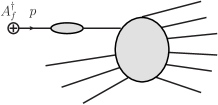
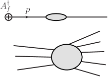
(a)	(b)	(c)

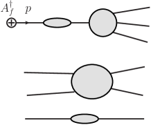
(d)	(e)

Figure 9: Showing examples of connectivity structure for a matrix element of $A_{f}^{\dagger}(t;\Delta t)$ and the Green function corresponding to it, with $n^{\prime}=3$ and $n=6$.

First, consider a component connected to $\tilde{\phi}(p)$ that has one or more particles in the initial state. The $\tilde{F}$ factor enforces that up to strongly suppressed contributions, $p$ is close to mass shell; the suppression is the same for all final states, so it will also apply to the sum and integral over states in (160). It also ensures that components without at least two particles in the final-state are suppressed, by the requirements for a momentum-conserving on-shell process.

The momentum conservation delta function removes the integral over $p$, leaving an integral over the $p_{j}$. Then the phase factor is

$$e^{-i(E_{\boldsymbol{p}}-p^{0})t}=\exp\mathopen{}\left[-it\left(E_{\sum\boldsymbol{q}_{k}-\sum\boldsymbol{p}_{j}}-\sum E_{\boldsymbol{q}_{k}}+\sum E_{\boldsymbol{p}_{j}}\right)\right].$$ (162)

The argument in Sec. XI.4 shows that a small deformation on the integral over the initial state momenta gives the relevant connected component of (159) as the limit. There are bounds on the errors that are uniform in the final state.

The remaining case is where there is a connected component with zero particles in the initial state. This corresponds to the example calculations that we performed in Secs. IX.3 and X for the LSZ operators and for the modified operators. When there is more than one particle in the final state, e.g., the first factor in Fig. 9(d), we get a strong suppression caused by the $\tilde{F}$ factor, unlike the case for the LSZ operator. The suppression is uniform in the final state.

There remains the expected one-particle case, as in the first factor in Fig. 9(b). Momentum conservation between $p$ and the single initial particle ensures that the phase factor and the $\tilde{F}$ factor are both unity.

The overall result is then a strong limit:

$$A^{\dagger}_{f;\,{\rm in}}\,|f_{1},\dots,f_{n^{\prime}};\,{\rm in}\rangle,=\lim_{\begin{subarray}{c}\rm infinite\\ \rm past\\ \rm time\end{subarray}}A_{f}^{\dagger}(t;\Delta t)\,|f_{1},\dots,f_{n^{\prime}};\,{\rm in}\rangle,=|f,f_{1},\dots,f_{n^{\prime}};\,{\rm in}\rangle.$$ (163)

A similar derivation applies to the final state for the creation operators for outgoing particles.

XII.2 Strong limit for in-annihilation operator

Next we consider the operator $A_{f}(t,\Delta t)$ in the infinite past, where it is intended to annihilate one particle. The equation for the matrix element is obtained by a minor modification of (XII.1):

$$\langle\boldsymbol{q}_{1},\dots,\boldsymbol{q}_{n};\,{\rm out}|\,A_{f}(t;\Delta t)\,|f_{1},\dots,f_{n^{\prime}};\,{\rm in}\rangle$$

$$={} \frac{1}{c}\int\frac{\mathop{{\mathrm{d}}^{4}{}q}\nolimits}{(2\pi)^{4}}\,\tilde{f}^{*}(\boldsymbol{q})\,\frac{E_{\boldsymbol{q}}+q^{0}}{2E_{\boldsymbol{p}}}\,e^{i(E_{\boldsymbol{q}}-q^{0})t}\,\tilde{F}^{*}(q^{0}-E_{\boldsymbol{q}},\Delta t)\,\langle\boldsymbol{q}_{1},\dots,\boldsymbol{q}_{n};\,{\rm out}|\,\tilde{\phi}(-q)\,|f_{1},\dots,f_{n^{\prime}};\,{\rm in}\rangle$$

$$={} \frac{1}{c}\int\prod_{j=1}^{n^{\prime}}\mathop{\widetilde{\mathop{{\mathrm{d}}{}p_{j}}\nolimits}}\nolimits\prod_{j=1}^{n^{\prime}}\tilde{f}_{j}(\boldsymbol{p}_{j})\int\frac{\mathop{{\mathrm{d}}^{4}{}q}\nolimits}{(2\pi)^{4}}\,\tilde{f}^{*}(\boldsymbol{q})\,\frac{E_{\boldsymbol{q}}+q^{0}}{2E_{\boldsymbol{q}}}\,e^{i(E_{\boldsymbol{q}}-q^{0})t}\,\tilde{F}^{*}(q^{0}-E_{\boldsymbol{q}},\Delta t)\times$$

$$\hskip 199.16928pt\times\,\langle\boldsymbol{q}_{1},\dots,\boldsymbol{q}_{n};\,{\rm out}|\,\tilde{\phi}(-q)\,|\boldsymbol{p}_{1},\dots,\boldsymbol{p}_{n^{\prime}};\,{\rm in}\rangle.$$ (164)

Here the momentum $q$ is defined to flow out of the corresponding Green function, as appropriate for an operator that is intended to destroy one of the initial-state particles. We will highlight the changes with the calculation for the creation operator. Unchanged is that $\tilde{F}$ strongly restricts $q$ to on-shell momentum, but now with positive energy flowing out of the Green function. Examples of the connectivity structure are shown in Fig. 10.

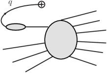
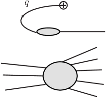
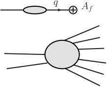
(a)	(b)	(c)

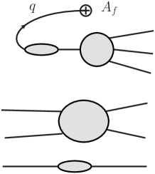
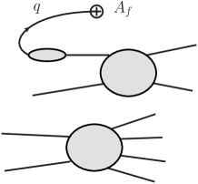
(d)	(e)

Figure 10: Showing examples of connectivity structure for a matrix element of $A_{f}(t;\Delta t)$ and the Green function corresponding to it, with $n^{\prime}=3$ and $n=6$. This is the same as Fig. 9, except that graphs are reoriented for the vertex for $A_{f}$ to emphasize its purpose as an annihilation operator.

Consider first a connected component with at least one initial particle and at least one final particle.

In the derivation of the reduction formula we used this annihilation operator at large positive time. The contour deformation to make $e^{i(E_{\boldsymbol{q}}-q^{0})t}$ suppressed on the deformed contour crossed the pole in the propagator, and picked out the pole contribution. But now with the opposite sign of $t$, the contour deformation is in the opposite direction, so the contribution is suppressed, with a suppression uniform in the final state. This result is illustrated by the following limit of Eq. (147):

$$\lim_{\begin{subarray}{c}t\to-\infty\\ \Delta t\to\infty\\ \Delta t/|t|\to 0\end{subarray}}\int\frac{\mathop{{\mathrm{d}}{}\delta E}\nolimits}{2\pi}e^{-i\delta E\,t}\tilde{F}(\delta E,\Delta t)\frac{i}{\delta E+i\epsilon}=0.$$ (165)

All other connected factors have no particles in either the initial or the final states. The $\tilde{F}$ factor suppresses all of them with one exception. The exception is a component with one initial particle and no final particle, i.e., of the form

$$\langle 0|\,A_{f}(t;\Delta t)\,|f_{1};\,{\rm in}\rangle,$$ (166)

illustrated by the first factor in Fig. 10(c).

Because the single particle is on-shell, there is no longer a phase factor. Instead we just get $\int\mathop{\widetilde{\mathop{{\mathrm{d}}{}p}\nolimits}}\nolimits\tilde{f}^{*}(\boldsymbol{p})\tilde{f}_{1}(\boldsymbol{p})$, as in the calculations in Sec. X. Observe that this is even independent of $t$ and $\Delta t$.

The overall result is that in the limit of infinite time in the past, the operator annihilates one incoming particle, and that the limit is a strong limit:

$$A_{f;\,{\rm in}}\,|f_{1},\dots,f_{n^{\prime}};\,{\rm in}\rangle=\lim_{\begin{subarray}{c}\rm infinite\\ \rm past\\ \rm time\end{subarray}}A_{f}(t;\Delta t)\,|f_{1},\dots,f_{n^{\prime}};\,{\rm in}\rangle=\sum_{j=1}^{n^{\prime}}|f_{1},\dots,f_{n^{\prime}},\text{with {\hbox{f_j}} omitted};\,{\rm in}\rangle\int\mathop{\widetilde{\mathop{{\mathrm{d}}{}p}\nolimits}}\nolimits\tilde{f}^{*}(\boldsymbol{p})\tilde{f}_{j}(\boldsymbol{p}).$$ (167)

XII.3 Comparison with LSZ

Let us now compare with the situation for the LSZ operators $a_{f}^{\dagger}(t)$. For the LSZ operators, the on-shell condition for a created or annihilated particle, i.e., for $p$ or $q$, was obtained from an integration over a rapidly oscillating phase factor identical with the one in (XII.1) or (XII.2). With the new operators, the on-shell condition is imposed more robustly by the $\tilde{F}$ factors. (The comparison between the two cases is assisted by observing that matrix elements of the LSZ operators can be obtained from those for the new operators simply by omitting the $\tilde{F}$ factor, or alternatively by setting $\Delta t=0$.)

In all but one case, the suppression in the LSZ case can be obtained by integrating over the momenta in the initial state. The one exception is where we have a connected component with no initial-state particles. This is exactly the situation explored by an explicit calculation in Sec. IX.3.2, and more generally in Sec. IX.4. In this case, momentum conservation between $p$ or $q$ and the external particles results in a phase factor that depends only on final-state momenta. Then an integral over final-state momenta is needed to get a suppression from the oscillations in the phase factor. Without the integral, there is no suppression, and hence we have a weak limit, but not a strong limit for the operators: The phase factor cancels in the integral over final states in (160).

XII.4 Commutation relations

Given now that the strong limits exist for the annihilation and creation operators, and that they have the expected action on in-states, it is elementary to derive the commutators.

For $A_{f;\,{\rm in}}^{\dagger}$ and $A_{g;\,{\rm in}}^{\dagger}$ we have

$$A_{f;\,{\rm in}}^{\dagger}A_{g;\,{\rm in}}^{\dagger}|f_{1},\dots,f_{n^{\prime}};\,{\rm in}\rangle=|f,g,f_{1},\dots,f_{n^{\prime}};\,{\rm in}\rangle.$$ (168)

Now the states are symmetric under exchange of the labels (as follows via the reduction formula from a corresponding property of Green functions). So we get the same result by applying the operators in the reverse order. Hence the operators commute:

$$[A_{f;\,{\rm in}}^{\dagger},A_{g;\,{\rm in}}^{\dagger}]=0.$$ (169)

For the commutator of two annihilation operators, the derived result for the action of an annihilation operator shows that two of them commute.

For one annihilation and one creation operator, we obtain the standard commutator:

$$[A_{f;\,{\rm in}},A_{g;\,{\rm in}}^{\dagger}]=\int\mathop{\widetilde{\mathop{{\mathrm{d}}{}p}\nolimits}}\nolimits\tilde{f}^{*}(\boldsymbol{p})\tilde{f}_{j}(\boldsymbol{p}).$$ (170)

XIII Generalizations

Various extensions and generalizations of the derived results are quite immediate:

1. The precise form of $F$ is irrelevant if it satisfies the same general specifications.

2. The same argument can be applied in any theory with any number of kinds of particle.

3. The field used in the Green function for a particular particle can be any field that has a nonzero matrix element between the vacuum and a state of one of that kind of particle. This generally means that the field should “have quantum numbers corresponding to the particle”. (E.g., for a proton we could use an operator with two anti-upquark fields and one anti-downquark field. These would be antiquark fields, because with the definition in (57), the fields need to be those that have the correct quantum numbers to create the particle.)

4. In this context the jargon is that the field is an “interpolating field” for the particle.

5. The choice of interpolating field is not unique. Thus in $\phi^{4}$ theory, $\phi^{3}$ or $\partial\phi/\partial x^{\mu}$ would work as interpolating fields instead of $\phi$, but at the expense of complication compared with the use of the elementary field.

6. The coefficient $c$ in the vacuum-to-one-particle matrix element generally depends on both the kind of particle and the field used. It is in general complex; given a particular type of particle, the phase can be eliminated by convention only for one field.

For another example of an interpolating field, consider a Schrödinger field theory of an electron field and a proton field, with a Coulomb interaction. This theory has single particle states not only for electrons and protons but also for every stable energy level of hydrogen atom, and in fact for any stable ion and molecule. A possible interpolating field for $s$-states of hydrogen would be $\psi^{\dagger}_{e}(t,\boldsymbol{x})\psi^{\dagger}_{p}(t,\boldsymbol{x})$. By choice of different time-dependent wave functions in the derivation of the LSZ formula we can pick out different energy levels of the atom for the particle that appears in an S-matrix element. If we want to deal with all energy levels, and not just $s$-states, one could separate the electron and proton fields: $\psi^{\dagger}_{e}(t,\boldsymbol{x}+\boldsymbol{y})\psi^{\dagger}_{p}(t,\boldsymbol{x}-\boldsymbol{y})$.

Particularly notable applications in strong interactions are for pseudo-scalar mesons like the pion, since for the pion, certain Noether currents for symmetries can be used as interpolating fields. Interesting results can be found be applying Ward identities for the symmetries to the Green functions used in the LSZ formula. This gets into the subject known as “current algebra”.

XIV Relation to Haag-Ruelle

In the formulation of Haag [4, 5] and Ruelle [6] the aim was to find a time-dependent operator that when applied to the vacuum it creates a single particle. They show that in an infinite-time limit products of such operators applied to the vacuum create general in- and out-states with desired wave functions. However they were concerned with general proofs rather than providing, for example, fully explicit constructions of the operators in a form useful for calculations in both coordinate and momentum space. Indeed Ruelle even states that Haag’s results are “less powerful than those of LSZ”: in contrast the formulation in the present paper are intended to be more powerful than LSZ.

The formulation given in the present paper organizes the construction of creation operators in a different way. It starts from the LSZ definition of a creation operator, which only has a spatial integral over a product of field and wave function and no time integral. This is then modified by an average over time. In contrast the Haag-Ruelle formulation, the order of the averaging and the integration with a wave function are reversed. Moreover, the averaging is over space-time, not just over time.

In the Haag-Ruelle method, the starting point is an “almost local” field defined by averaging $\phi$ with a test function $h$:

$$\phi_{h}(x)=\int\mathop{{\mathrm{d}}^{4}{}y}\nolimits\,h(x-y)\,\phi(y).$$ (171)

Then a candidate creation operator is defined by applying the formula for $a_{f}^{\dagger}(t)$ to $\phi_{h}(x)$ instead of to $\phi(x)$:

$$a_{f,h}^{\dagger}(t)=-i\int\mathop{{\mathrm{d}}^{3}{}\boldsymbol{x}}\nolimits\,f(x)\overleftrightarrow{\frac{\partial}{\partial t}}\phi_{h}(x).$$ (172)

Given the Fourier transform of $h$,

$$h(x-y)=\int\frac{\mathop{{\mathrm{d}}^{4}{}p}\nolimits}{(2\pi)^{4}}\,\tilde{h}(p)\,e^{ip\cdot(x-y)},$$ (173)

the momentum-space expression for $a_{f}^{\dagger}(t)$ is

$$a_{f,h}^{\dagger}(t)=\int\mathop{\widetilde{\mathop{{\mathrm{d}}{}p}\nolimits}}\nolimits\tilde{f}(\boldsymbol{p})\int\frac{\mathop{{\mathrm{d}}{}p^{0}}\nolimits}{2\pi}\times\\ \times\tilde{\phi}(p)\,\tilde{h}(p)\,(E_{\boldsymbol{p}}+p^{0})\,e^{-i(E_{\boldsymbol{p}}-p^{0})t}.$$ (174)

To enable this operator to create a single-particle state of specified momentum content, but no multi-particle component, a restriction is made on the support of $\tilde{h}(p)$. Thus Duncan [2] required the support confined to a region $am_{\rm phys}^{2}<p^{2}<bm_{\rm phys}^{2}$ with $0<a<1$ and $1<b<4$, and that the function be non-zero on the whole of the one-particle mass shell, where $p^{0}=\sqrt{\boldsymbol{p}^{2}+m_{\rm phys}^{2}}$. In addition, $\tilde{h}(p)$ is zero when $p^{0}$ is negative. Given the known matrix element of the field between the vacuum and the one-particle states, it follows that the state created by $a_{f,h}^{\dagger}(t)$ acting on the vacuum is

$$a_{f,h}^{\dagger}(t)|0\rangle=\int\mathop{\widetilde{\mathop{{\mathrm{d}}{}p}\nolimits}}\nolimits\,\tilde{h}(E_{\boldsymbol{p}},\boldsymbol{p})\,\tilde{f}(\boldsymbol{p})\,|\boldsymbol{p}\rangle.$$ (175)

As usual with test functions, $\tilde{h}(p)$ is both infinitely differentiable and decreases faster than any power of $p$ when $p$ gets large. Since therefore $\tilde{h}(E_{\boldsymbol{p}},\boldsymbol{p})$ cannot be a constant everywhere, the state differs from the one with wave function $\tilde{f}(\boldsymbol{p})$. Nevertheless, given any desired normalizable single particle state, it can be created by suitably choosing $\tilde{f}(\boldsymbol{p})$ in (175), i.e., by replacing $\tilde{f}$ by $\tilde{f}(\boldsymbol{p})/\tilde{h}(E_{\boldsymbol{p}},\boldsymbol{p})$. (A slightly different formulation with the same aim was given by Hepp [7].)

However what is not provided in this formalism is a simple formula involving an integral of the coordinate-space field to give exactly the one-particle state of a particular target wave function $|f\rangle$.

In contrast, the formulation in the present paper has reversed the order of the averaging operation and the integration with the wave function $f$, and has also made the averaging function a function of time only. For this to work, stronger dynamical requirements are imposed on large momentum behavior of matrix elements than in the Haag-Ruelle formulation. These requirements are certainly valid in the renormalizable QFTs that we are normally interested in, at least as regards what can be seen in perturbation theory. The Haag-Ruelle method comes from a tradition that deliberately aims to derive general properties of a relativistic QFT without appealing to more detailed dynamical properties that generally are consequences of particular QFTs.

A further difference compared with the Haag-Ruelle method is that the operators $A_{f}^{\dagger}(t,\Delta t)$ defined in the present paper, have a second parameter $\Delta t$ that also has to be taken to infinity. This change is what enables explicit calculationally useful formulas to be given in both coordinate and momentum space—see Eq. (IX.5). The extra parameter has a useful interpretation in terms of an energy uncertainty, and physically should correspond to the experimental realities of making beams of particles of almost exactly given momenta. The explicit coordinate-space formula for $A_{f}^{\dagger}(t,\Delta t)$, together with the new proof of the reduction formula, are intended to be useful for further applications, e.g., to the treatment of unstable particles, as in Ref. [12].

The strong commonalities between the Haag-Ruelle and the new methods are that they perform some kind of averaging of the operators that brings in an integral over time, and that the nature of the averaging is arranged to restrict the momentum-space support of the creation operator to correspond exactly to a single particle. That is, the coupling to multi-particle states is arranged to be zero by construction of the definition (assisted by a limiting operation).

Appendix A Strong v. weak limits, etc

In treatments of scattering theory, we often discuss limits of operators as a time parameter goes to infinity. It is useful to distinguish three kinds of definition of a statement that $\lim_{t\to\infty}A(t)=B$, where $A(t)$ and $B$ are linear operators on the state space of a theory:

• A very strong limit is where some measure of the difference between the operators $A(t)$ and $B$ themselves goes to zero:

  $$\|A(t)-B\|\to 0.$$ (176)

  Here the measure of the size of $A(t)-B$ does not depend on the states acted on. The name is coined here. As will be pointed out below, limits of this kind typically do not exist for the operators used in the analysis of scattering.

• A strong limit is where the limit applies to states:

  $$\left\|\left(A(t)-B\right)|f\rangle\right\|\to 0,$$ (177)

  for each state $|f\rangle$, but where the approach to the limit is permitted to depend on the state.

• A weak limit is where the limit is only for matrix elements

  $$\left|\langle g|\left(A(t)-B\right)|f\rangle\right|\to 0,$$ (178)

  for each pair of normalizable states $|f\rangle$ and $\langle g|$, but where the approach to the limit is permitted to depend on the states.

The existence of a very strong limit implies the existence of the strong and weak limits, and the existence of a strong limit implies the existence of a weak limit. But the reverse implications are false.

The existence of a very strong limit is equivalent to saying that the approach of $\langle g|A(t)|f\rangle$ to $\langle g|B|f\rangle$ is uniform in both of the states $\langle g|$ and $|f\rangle$. The existence of a strong limit is equivalent to uniformity in $|f\rangle$ only.

Generally, in applications such as to evolution operators, creation operators, and the like in scattering theory, very strong limits do not exist. This is simply because we use theories that are invariant under time translations. Therefore (Heisenberg-picture) states may be constructed that correspond to a physical scattering that occurs arbitrarily far in the past or future. How far in time one has to go to get an approximation that corresponds to separated incoming or outgoing particles depends on when the scattering(s) occur, and no fixed time independent of the state suffices. Thus very strong limits do not exist in such cases.

Calculational methods (e.g., perturbation theory) lend themselves naturally to the calculation of matrix elements rather than of the operators themselves. So it is useful to make definitions of the different kinds of limit in terms of matrix elements, both with normalized states and with states of particles of definite momenta. Moreover the matrix elements are typically between an in and an out state, i.e., in using the definitions, we would normally replace $|f\rangle$ by $|\underline{f};\,{\rm in}\rangle$, and $|g\rangle$ by $|\underline{g};\,{\rm out}\rangle$, with $\underline{f}$ and $\underline{g}$ denoting specifications of in- and out-states in terms of their particle content, with the notation of Sec. IV.4.

All the criteria for the different limits can be expressed in terms of

$$\epsilon_{\rm ME}(t,f,g)\stackrel{{\scriptstyle\textrm{def}}}{{=}}\frac{\left|\langle g|(A(t)-B)|f\rangle\right|}{\||g\rangle\|~{}\||f\rangle\|}.$$ (179)

Here there is a factor of the norms of the states in the denominator to make the quantity invariant under scaling of the states.

The definition that the weak limit exists is simply the statement that $\epsilon_{\rm ME}(t,f,g)\to 0$ as $t\to\infty$ for each $f$ and $g$.

Now the Cauchy-Schwartz inequality implies that

$$\left|\langle g|(A(t)-B)|f\rangle\right|\,\leq\,\||g\rangle\|~{}\|(A(t)-B)|f\rangle\|,$$ (180)

with equality only when $|g\rangle$ is proportional to $(A(t)-B)|f\rangle$. So

$$\epsilon_{\rm ME}(t,f,g)\leq\frac{\|(A(t)-B)|f\rangle\|}{\||f\rangle\|}.$$ (181)

This immediately shows that if the strong limit exists, so does the weak limit.

Typically the proofs of existence of a limit are first made for $t\to\infty$ of the matrix element with fixed states, with a finding that the weak limit exists. Then a possible approach to determining whether in addition the strong limit exists is to find an upper bound to $\epsilon_{\rm ME}(t,f,g)$ as $g$ is varied with $|f\rangle$ fixed. So we define

$$\epsilon_{\rm state}(t,f) \stackrel{{\scriptstyle\textrm{def}}}{{=}}\sup_{\text{non-zero }|g\rangle}\epsilon_{\rm ME}(t,f,g)$$

$$=\sup_{\text{non-zero }|g\rangle}\frac{|\langle g|(A(t)-B)|f\rangle}{\||g\rangle\|~{}\||f\rangle\|}.$$ (182)

(Here we use the notation for the supremum, i.e., the least upper bound.) We have already seen that the right-hand side is the same as $\|(A(t)-B)|f\rangle\|/\||f\rangle\|$. So if we can bound $\epsilon_{\rm state}(t,f)$ on the basis of matrix element calculations and show that it goes to zero as $t\to\infty$, then we know that the strong limit exists.

Now, in calculations and proofs we often express a matrix element in terms of an integral over momenta — see Secs. IX.3.5 and XI, for example. Then the $t$ dependence appears as a phase, which commonly oscillates infinitely rapidly as $t\to\infty$. The limit then commonly involves strong cancellations because of the oscillations, as in the weak limits of the LSZ operator $a_{f}^{\dagger}(t)$. Then for a given value of $t$, we may be able to change the state $|g\rangle$ to another state $|g_{t,f}\rangle$ that has the same norm and in which the wave functions are given phases that cancel the first-mentioned phase. See Sec. IX.3.5 for an example.

In this situation, since all possible states $|g\rangle$ are allowed in calculating the bound in Eq. (A), we therefore find that $\epsilon_{\rm state}(t,f)$ is independent of $t$, and hence that the strong limit does not exist.

Another approach is convenient when we specify $|f\rangle$ as an in-state, is to express the norm of $(A(t)-B)|f;\,{\rm in}\rangle$ in terms of basis out-states of particles of definite momenta:

$$\|(A(t)-B)|f;{\rm in}\rangle\|^{2}\\ =\operatorname*{\mathchoice{\ooalign{$\displaystyle\sum$\cr$\displaystyle\int$\cr}}{\ooalign{\raisebox{0.14pt}{\scalebox{0.7}{$\textstyle\sum$}}\cr$\textstyle\int$\cr}}{\ooalign{\raisebox{0.2pt}{\scalebox{0.6}{$\scriptstyle\sum$}}\cr$\scriptstyle\int$\cr}}{\ooalign{\raisebox{0.2pt}{\scalebox{0.6}{$\scriptstyle\sum$}}\cr$\scriptstyle\int$\cr}}}\mathop{{\mathrm{d}}{}X}\nolimits\left|\langle X;\,{\rm out}|(A(t)-B)|f;{\rm in}\rangle\right|^{2}.$$ (183)

Here the integral over $X$ is a sum and integral over all out-basis states, and includes the appropriate normalization factor. Consider now the situation (as with the LSZ operators) that the weak limit with normalizable states relies on a cancellation of rapid oscillations of a momentum-dependent phase factor, and that this needs an integral over wave functions for both the initial and final states. In the absolute value of a matrix element with a momentum eigenstate, as in the right-hand side of Eq. (183), the phase is replaced by unity. Then we no longer have a suppression as $t\to\infty$. A typical example of this situation was shown in Sec. IX.3.2.

Finally, we come to the possible existence of a very strong limit. Let us define the size of the difference between the operators $A(t)$ and $B$ in terms of matrix elements by

$$\|A(t)-B\| =\epsilon_{\rm op}(t)$$

$$\stackrel{{\scriptstyle\textrm{def}}}{{=}}\sup_{\text{non-zero }|f\rangle,|g\rangle}\frac{\left|\langle g|(A(t)-B)|f\rangle\right|}{\||g\rangle\|~{}\||f\rangle\|}$$

$$=\sup_{\text{non-zero }|f\rangle,|g\rangle}\epsilon_{\rm ME}(t,f,g)$$

$$=\sup_{\text{non-zero }|g\rangle}\epsilon_{\rm state}(t,f).$$ (184)

The variety of forms for this definition relates the size of difference of operators to the formulas we used for the determining the existence of weak and strong limits.

First these results show explicitly that if the very strong limit exists, then so do the strong and weak limits.

We also see how it may happen that the strong and weak limits exist, but the very strong limit can be shown not to exist. Suppose, as is usual in this context, that the $t$ dependence is confined to a phase factor in momentum-space integral and that the integrand contains factors of momentum-space wave functions. Then we may be able to cancel the phase by changing the states to certain other states $|f_{t}\rangle$ and $|g_{t}\rangle$ with appropriate $t$-dependent phases in their momentum-space wave functions, and hence unchanged norms. Such is the case in the derivation of the reduction formula, where the $t$-dependent phases in Eq. (XI.3) can be canceled by changing the wave functions. Then $\langle g_{t}|(A(t)-B)|f_{t}\rangle$ is independent of time, and so

$$\|A(t)-B\| \geq\frac{\left|\langle g_{t}|(A(t)-B)|f_{t}\rangle\right|}{\||g_{t}\rangle\|\,\||f_{t}\rangle\|}$$

$$=\frac{\left|\langle g|(A(0)-B)|f\rangle\right|}{\||g\rangle\|\,\||f\rangle\|},$$ (185)

which is nonzero. Then $\|A(t)-B\|$ cannot go to zero as $t\to\infty$, and therefore in this case, the very strong limit does not exist. As already mentioned, the non-existence of a very strong limit is to be expected in a time-translationally invariant theory; the approach to an infinite-time limit is controlled by the time relative to a scattering event, and the time of a scattering depends on the state considered.

References

- Lehmann et al. [1955] H. Lehmann, K. Symanzik, and W. Zimmermann, On the formulation of quantized field theories, Nuovo Cim. 1, 205 (1955).
- Duncan [0012] A. Duncan, The Conceptual Framework of Quantum Field Theory (Oxford University Press, Oxford, 20012).
- Goldberger and Watson [1964] M. L. Goldberger and K. M. Watson, Collision Theory (Wiley, 1964).
- Haag [1958] R. Haag, Quantum field theories with composite particles and asymptotic conditions, Phys. Rev. 112, 669 (1958).
- Haag [1959] R. Haag, The framework of quantum field theory, Suppl. Nuovo Cim. 14, 131 (1959).
- Ruelle [1962] D. Ruelle, On the asymptotic condition in quantum field theory, Helv. Phys. Acta 35, 147 (1962).
- Hepp [1965] K. Hepp, On the connection between the LSZ and Wightman quantum field theory, Comm. Math. Phys. 1, 95 (1965).
- Akhmedov [2019] E. Akhmedov, Quantum mechanics aspects and subtleties of neutrino oscillations (2019) arXiv:1901.05232 [hep-ph] .
- Akhmedov and Kopp [2010] E. K. Akhmedov and J. Kopp, Neutrino oscillations: Quantum mechanics vs. quantum field theory, JHEP 04, 008, [Erratum: JHEP10,052(2013)], arXiv:1001.4815 [hep-ph] .
- Coleman [2011] S. Coleman, Notes from Sidney Coleman’s Physics 253a: Quantum Field Theory, arXiv:1110.5013 [physics.ed-ph] .
- Chen et al. [2018] B. G.-g. Chen, D. Derbes, D. Griffiths, B. Hill, R. Sohn, and Y.-S. Ting, Lectures of Sidney Coleman on Quantum Field Theory (World Scientific, 2018) https://www.worldscientific.com/doi/pdf/10.1142/9371 .
- Boyanovsky [2019] D. Boyanovsky, Quantum decay in renormalizable field theories: quasiparticle formation, Zeno and anti-Zeno effects, Annals Phys. 405, 176 (2019), arXiv:1810.01301 [hep-th] .
- Kapec et al. [2017] D. Kapec, M. Perry, A.-M. Raclariu, and A. Strominger, Infrared Divergences in QED, Revisited, Phys. Rev. D96, 085002 (2017), arXiv:1705.04311 [hep-th] .
- Hoare et al. [2018] B. Hoare, N. Levine, and A. A. Tseytlin, On the massless tree-level S-matrix in 2d sigma models, arXiv:1812.02549 [hep-th] .
- Zamolodchikov and Zamolodchikov [1992] A. B. Zamolodchikov and A. B. Zamolodchikov, Massless factorized scattering and sigma models with topological terms, Nucl. Phys. B379, 602 (1992).
- Born and Jordan [1925] M. Born and P. Jordan, Zur Quantenmechanik, Zeit. f. Phys. 34, 858 (1925), English translation in Ref. [33], but without the last section (on the quantized electromagnetic field).
- van Hove [1951] L. van Hove, Sur l’opérateur Hamiltonien de deux champs quantifiés en interaction, Bulletin de la Classe des Sciences Academie Royale de Belgique 37, 1055 (1951).
- van Hove [1952] L. van Hove, Les difficultés de divergences pour un modèle particulier de champ quantifié, Physica 18, 145 (1952).
- Haag [1955] R. Haag, On quantum field theories, Kong. Dan. Vid. Sel. Mat. Fys. Med. 29, 1 (1955), [Phil. Mag. Ser.746,376(1955)].
- Streater and Wightman [1964] R. F. Streater and A. S. Wightman, PCT, spin and statistics, and all that (W. A. Benjamin, 1964).
- Sterman [1993] G. Sterman, An Introduction to Quantum Field Theory (Cambridge University Press, Cambridge, 1993).
- Srednicki [2007] M. Srednicki, Quantum Field Theory (Cambridge University Press, Cambridge, 2007).
- Peskin and Schroeder [1995] M. E. Peskin and D. V. Schroeder, An Introduction to Quantum Field Theory (Addison-Wesley, Reading, MA, 1995).
- Jain [2007] J. K. Jain, Composite Fermions (Cambridge University Press, Cambridge, 2007).
- Weinberg [1995] S. Weinberg, The Quantum Theory of Fields, Vol. I, Foundations (Cambridge University Press, Cambridge, 1995).
- Taylor [1972] J. R. Taylor, Scattering Theory: The Quantum Theory of Nonrelativistic Collisions (Wiley, 1972).
- Itzykson and Zuber [1980] C. Itzykson and J.-B. Zuber, Quantum Field Theory (McGraw-Hill, New York, 1980).
- Källén [1952] G. Källén, On the definition of the Renormalization Constants in Quantum Electrodynamics, Helv. Phys. Acta 25, 417 (1952), [,509(1952)].
- Lehmann [1954] H. Lehmann, On the Properties of propagation functions and renormalization contants of quantized fields, Nuovo Cim. 11, 342 (1954).
- Bogoliubov and Shirkov [1959] N. N. Bogoliubov and D. V. Shirkov, Introduction to the Theory of Quantized Fields (Wiley-Interscience, New York, 1959).
- Bjorken and Drell [1965] J. D. Bjorken and S. D. Drell, Relativistic quantum fields (McGraw-Hill, 1965).
- Schlieder and Seiler [1972] S. Schlieder and E. Seiler, Remarks on the null plane development of a relativistic quantum field theory, Commun. Math. Phys. 25, 62 (1972).
- Van Der Waerden [1967] B. Van Der Waerden, Sources of Quantum Mechanics (North-Holland, 1967).