KUNS-2760

A $\mu$-$\tau$-philic scalar doublet under $Z_{n}$ flavor symmetry

Yoshihiko Abe¹ , Takashi Toma^1,2 , Koji Tsumura¹

¹Department of Physics, Kyoto University, Kyoto 606-8502, Japan
²Department of Physics, McGill University,
3600 Rue University, Montréal, Québec H3A 2T8, Canada

1 Introduction

The Standard Model (SM) has been established by the discovery of the Higgs boson at the LHC. New particles beyond the SM are also being searched at the LHC. However, there is no signature of new particles until now, and the experimental results are consistent with the SM predictions. Other than the high energy frontier experiment, many of flavor observables are measured very precisely as the luminosity frontier experiment. A striking indication of the beyond the SM would be the muon anomalous magnetic moment (muon $g-2$). There is a discrepancy between the measured value and the SM prediction as [1]

$$\Delta a_{\mu}=a_{\mu}^{\mathrm{exp}}-a_{\mu}^{\mathrm{SM}}=268(63)(43)\times 10^{-11},$$ (1)

where the numbers in the first and second parentheses represent the statistical and systematic errors, respectively. The total significance of the deviation is $3.5\sigma$ far from the SM prediction. Note that there is a non-negligible large theoretical uncertainties in the hadronic contribution due to the light-by-light scattering [3]. Currently, FNAL E989 experiment is ongoing, and will achieve a factor four improvement on its precision at the end of the running [4].

There are many attempts to explain the discrepancy of the muon magnetic moment. For instance, in lepton-specific two Higgs doublet models (THDMs), the new contribution to the muon magnetic moment due to the additional Higgs bosons can be enhanced by a large $\tan\beta$, which is the ratio of vacuum expectation values (VEVs) of two Higgs doublets [7, 6, 5, 8]. The THDM with tree-level flavor changing neutral currents has also been studied to explain the discrepancy in the light of the $h\to\mu\tau$ excess at the LHC [9, 10], which has been disappeared. Another way is to consider a light $Z^{\prime}$ gauge boson associated with an extra $U(1)_{{\mathbf{L}}_{\mu}-{\mathbf{L}}_{\tau}}$ symmetry [11, 12], or a light hidden photon [13]. In these models, thanks to the new light mediator running in the loop diagram, the muon magnetic moment can be enhanced even with a smaller coupling strength. There is also argument to account for the discrepancy in framework of supersymmetry [14], axion-like particle [15] and fourth generation of leptons [16].

In this paper, we propose a minimal model explaining the discrepancy of the muon anomalous magnetic moment between the SM prediction and the measurement based on abelian discrete symmetries. Models based on the abelian discrete groups easily give a sufficiently large and the correct sign of the contribution to the muon magnetic moment. The model based on a $Z_{4}$ symmetry is identified as the minimal model, which is a kind of variant of the inert scalar doublet model based on a $Z_{2}$ symmetry. Thanks to the $Z_{4}$ symmetry, the lepton flavor violating (LFV) processes such as $\ell\to\ell^{\prime}\gamma~{}(\ell,\ell^{\prime}=e,\mu,\tau)$ are forbidden automatically against severe bounds of their non-observation. As a result, we find a solution to the muon $g-2$ anomaly without conflicting with the constraints from the electroweak precision tests and the lepton universality of heavy charged lepton decays and $Z$ boson leptonic decays. In addition, we examine whether the model is consistent with theoretical bounds of potential stability and triviality. We will formulate analytic expressions of these quantities, and numerically explore the parameter space which can accommodate the discrepancy of the muon anomalous magnetic moment. As further perspective, neutrino mass generation mechanism and a distinctive collider signature, a prediction for muon electric dipole moment induced by new CP phases and influence on the Higgs decay into $\gamma\gamma$ will also be discussed.

2 Flavor Charged Scalar Doublets

Let us discuss a simple extension of the SM with a pair of scalar doublets $(\Phi,\underline{\Phi}\,)$ whose global $U(1)_{{\mathbf{L}}_{\mu}-{\mathbf{L}}_{\tau}}$ flavor charge is $(2,-2)$, where ${\mathbf{L}}_{\mu}$ and ${\mathbf{L}}_{\tau}$ represent the muon and tau lepton flavor numbers, respectively. Detailed quantum charge assignments are given in Table 1.

Particle	SM	$U(1)_{{\mathbf{L}}_{\mu}-{\mathbf{L}}_{\tau}}$	$Z_{2}$	$Z_{3}$	$Z_{4}$	$Z_{n}$
$(L_{e},L_{\mu},L_{\tau})$	$(1,2)_{-1/2}$	$(0,+1,-1)$	$(+,-,-)$	$(1,\omega,\omega^{2})$	$(1,i,-i)$	$(1,\omega,\underline{\omega})$
$(e_{R},\mu_{R},\tau_{R})$	$(1,1)_{-1}$	$(0,+1,-1)$	$(+,-,-)$	$(1,\omega,\omega^{2})$	$(1,i,-i)$	$(1,\omega,\underline{\omega})$
$H$	$(1,2)_{1/2}$	$0$	$+$	$1$	$1$	$1$
$\Phi$	$(1,2)_{1/2}$	$+2$	$+$	$\omega^{2}$	$-1$	$\omega^{2}$
$\underline{\Phi}$	$(1,2)_{1/2}$	$-2$	$+$	$\omega$	$-1$	$\underline{\omega}^{2}$

Table 1: Particle contents of models based on $U(1)_{{\mathbf{L}}_{\mu}-{\mathbf{L}}_{\tau}}$ and $Z_{n}$ flavor symmetries. The quantum numbers of the SM are also shown in the notation of $\big{(}SU(3)_{c},SU(2)_{L}\big{)}_{U(1)_{Y}}$. For abelian discrete symmetry $Z_{n}$, $\underline{\omega}$ is a conjugate of $\omega$, where $\omega$ is $n$-th root of unity.

Under this flavor symmetry, the following new Yukawa interactions are allowed,

$$-{\mathcal{L}}_{U(1)}^{\text{yukawa}}=y_{\tau\mu}\,\Phi^{{\dagger}}\,\overline{\tau_{R}}\,L_{\mu}+\underline{y_{\mu\tau}}\,\underline{\Phi}^{{\dagger}}\,\overline{\mu_{R}}\,L_{\tau}+\text{H.c.}$$ (2)

in addition to the quartic scalar interaction term $(H^{{\dagger}}\Phi)(H^{{\dagger}}\underline{\Phi})$. These interactions easily generate sizable contributions to the muon $g-2$ by the scalar mediators as shown in Fig. 1. In the ordinary gauged $U(1)_{{\mathbf{L}}_{\mu}-{\mathbf{L}}_{\tau}}$ model, the discrepancy in the muon $g-2$ is explained by the new light $Z^{\prime}$ gauge boson [11, 12], while in our new proposals a pair of scalar doublets is introduced to give a sizable contribution to the muon $g-2$. A similar contribution to the muon $g-2$ from the scalar doublets are discussed in the model based on the $SU(2)_{\mu\tau}$ symmetry, which contains the $U(1)_{{\mathbf{L}}_{\mu}-{\mathbf{L}}_{\tau}}$ symmetry as a subgroup [17]. In such cases, a pair of scalar doublets plays the primary role in explaining the muon $g-2$ anomaly instead of $Z^{\prime}$ bosons. We noted that this new contribution remains even with the unbroken $U(1)_{{\mathbf{L}}_{\mu}-{\mathbf{L}}_{\tau}}$ flavor symmetry limit.

From the above consideration in our mind, we begin with a global $U(1)_{{\mathbf{L}}_{\mu}-{\mathbf{L}}_{\tau}}$ symmetry together with a pair of scalar doublets as a simple model for the muon $g-2$ anomaly. On the other hand, the $U(1)_{{\mathbf{L}}_{\mu}-{\mathbf{L}}_{\tau}}$ symmetry must be broken in order to realize observed neutrino masses and mixings [18]. If the $U(1)_{{\mathbf{L}}_{\mu}-{\mathbf{L}}_{\tau}}$ is not gauged, an experimentally unwanted Nambu-Goldstone boson emerges. To avoid this problem, we concentrate on abelian discrete symmetries $Z_{n}(n=2,3,\cdots)$, which break the $U(1)_{{\mathbf{L}}_{\mu}-{\mathbf{L}}_{\tau}}$ symmetry explicitly.

The Yukawa interactions based on $Z_{n}$ flavor symmetries are given by

$$-{\mathcal{L}}_{Z_{2}}^{\text{yukawa}} =\overline{\ell_{R}}\begin{pmatrix}y_{e}H^{{\dagger}}+y_{ee}\Phi^{{\dagger}}&&\\ &y_{\mu}H^{{\dagger}}+y_{\mu\mu}\Phi^{{\dagger}}&g_{\mu\tau}H^{{\dagger}}+y_{\mu\tau}\Phi^{{\dagger}}\\ &g_{\tau\mu}H^{{\dagger}}+y_{\tau\mu}\Phi^{{\dagger}}&y_{\tau}H+y_{\tau\tau}\Phi^{{\dagger}}\end{pmatrix}\!L+\text{H.c.}$$ (3)

$$-{\mathcal{L}}_{Z_{3}}^{\text{yukawa}} =\overline{\ell_{R}}\begin{pmatrix}y_{e}H^{{\dagger}}&\underline{y_{e\mu}}\underline{\Phi}^{{\dagger}}&y_{e\tau}\Phi^{{\dagger}}\\ y_{\mu e}\Phi^{{\dagger}}&y_{\mu}H^{{\dagger}}&\underline{y_{\mu\tau}}\underline{\Phi}^{{\dagger}}\\ \underline{y_{\tau e}}\underline{\Phi}^{{\dagger}}&y_{\tau\mu}\Phi^{{\dagger}}&y_{\tau}H^{{\dagger}}\end{pmatrix}\!L+\text{H.c.}$$ (4)

$$-{\mathcal{L}}_{Z_{4}}^{\text{yukawa}} =\overline{\ell_{R}}\begin{pmatrix}y_{e}H^{{\dagger}}&&\\ &y_{\mu}H^{{\dagger}}&y_{\mu\tau}\Phi^{{\dagger}}\\ &y_{\tau\mu}\Phi^{{\dagger}}&y_{\tau}H^{{\dagger}}\end{pmatrix}\!L+\text{H.c.}$$ (5)

$$-{\mathcal{L}}_{Z_{n\geq 5}}^{\text{yukawa}} =\overline{\ell_{R}}\begin{pmatrix}y_{e}H^{{\dagger}}&&\\ &y_{\mu}H^{{\dagger}}&\underline{y_{\mu\tau}}\underline{\Phi}^{{\dagger}}\\ &y_{\tau\mu}\Phi^{{\dagger}}&y_{\tau}H^{{\dagger}}\end{pmatrix}\!L+\text{H.c.}$$ (6)

The $Z_{n}$ charge assignment in each model is given in Table 1. For $n\geq 5$, an accidental global $U(1)_{{\mathbf{L}}_{\mu}-{\mathbf{L}}_{\tau}}$ symmetry is recovered in the Yukawa interactions taking into account renormalizability. Depending on the chosen abelian discrete flavor symmetry, a specific structure of the Yukawa interaction is predicted. Note that since $\underline{\Phi}$ is identical to $\Phi$ in the $Z_{2}$ and $Z_{4}$ models, the Yukawa interactions of $\underline{\Phi}$ are not shown for these models. In the following, we focus on the models with only one extra scalar doublet $\Phi$, which minimally explain the muon $g-2$ anomaly.

Figure 1: Feynman diagram inducing muon anomalous magnetic moment in $U(1)_{{\mathbf{L}}_{\mu}-{\mathbf{L}}_{\tau}}$ and $Z_{n}~{}(n=2,3,\cdots)$ models.

In the model based on $Z_{2}$ or $Z_{4}$, possible large new contributions to the muon $g-2$ are retained thanks to the existence of the quartic term $(H^{{\dagger}}\Phi)^{2}$. From the view of experimental constraints, the $Z_{4}$ model is more favorable because the $Z_{2}$ model predicts LFV processes $\tau\to 3\mu,e\mu\mu$ at tree-level, and thus parameter tuning is necessary to suppress these processes. On the other hand, the LFV processes are automatically forbidden in the (unbroken) $Z_{4}$ model. From the view of the numbers of parameters in the model, again the $Z_{4}$ model is preferable both in the Yukawa sector and the scalar potential. We therefore conclude that the model based on the $Z_{4}$ lepton flavor symmetry is the minimal scalar extension of the SM to accommodate the muon $g-2$ anomaly.

3 The Minimal Model for Muon $g-2$

Following the argument in the previous section, we introduce a new scalar doublet $\Phi$ to the SM, and impose a $Z_{4}$ symmetry. The $Z_{4}$ charge assignment is shown in Table 1, and all the other fields are trivial under the $Z_{4}$ symmetry. The invariant scalar potential is given by

$$\mathcal{V} =\mu_{H}^{2}|H|^{2}+\mu_{\Phi}^{2}|\Phi|^{2}+\lambda_{1}|H|^{4}+\lambda_{2}|\Phi|^{4}$$

$$~{}~{}~{}+\lambda_{3}|H|^{2}|\Phi|^{2}+\lambda_{4}|H^{{\dagger}}\Phi|^{2}+\left[\frac{\lambda_{5}}{2}\left(H^{{\dagger}}\Phi\right)^{2}+\mathrm{H.c.}\right].$$ (7)

This scalar potential is the same as that in the scalar inert doublet model [19], where an exact $Z_{2}$ symmetry is preserved in the potential. In general, the quartic coupling $\lambda_{5}$ and the Yukawa couplings $y_{\mu\tau}$, $y_{\tau\mu}$ are complex. One of the CP phases can be eliminated by the field redefinition of $\Phi$. Here, we remove the CP phase of $\lambda_{5}$ without loss of generality. Since we demand a stable vacuum, the potential should be bounded from below. The conditions for these requirements are known as  [20]

$$\lambda_{1}>0,\quad\lambda_{2}>0,\quad 2\sqrt{\lambda_{1}\lambda_{2}}+\lambda_{3}>0,\quad 2\sqrt{\lambda_{1}\lambda_{2}}+\lambda_{3}+\lambda_{4}\pm|\lambda_{5}|>0,$$ (8)

at tree level. The Higgs doublet $H$ develops a VEV as in the SM, and the electroweak symmetry is spontaneously broken. The new doublet scalar $\Phi$ is assumed to have a vanishing VEV at leading order. The scalar fields can then be parameterized as

$$H=\left(\begin{array}[]{c}0\\ \left(v+h\right)/\sqrt{2}\end{array}\right),\qquad\Phi=\left(\begin{array}[]{c}\phi^{+}\\ \left(\rho+i\eta\right)/\sqrt{2}\end{array}\right).$$ (13)

A component field $h$ corresponds to the Higgs boson with the mass $m_{h}=\sqrt{2\lambda_{1}}v=125~{}\mathrm{GeV}$. The electrically neutral component of $\Phi$, $\phi^{0}=(\rho+i\eta)/\sqrt{2}$, splits into the two mass eigenstates $\rho$ and $\eta$. The masses of these neutral states and charged component $\phi^{+}$ are given by

$$m_{\rho}^{2} =\mu_{\Phi}^{2}+\left(\lambda_{3}+\lambda_{4}+\lambda_{5}\right)\frac{v^{2}}{2},$$ (14)

$$m_{\eta}^{2} =\mu_{\Phi}^{2}+\left(\lambda_{3}+\lambda_{4}-\lambda_{5}\right)\frac{v^{2}}{2},$$ (15)

$$m_{\phi}^{2} =\mu_{\Phi}^{2}+\lambda_{3}\frac{v^{2}}{2}.$$ (16)

Thus, one can see that the mass splitting between $\rho$ and $\eta$ is controlled by the quartic coupling $\lambda_{5}$ via the relation $m_{\rho}^{2}-m_{\eta}^{2}=\lambda_{5}v^{2}$.

Figure 2: Feynman diagram inducing muon anomalous magnetic moment in $Z_{4}$ model.

In this model, the new contribution to muon anomalous magnetic moment comes from Fig. 2, which is computed as

$$\Delta a_{\mu}^{\mathrm{new}} =\frac{\mathrm{Re}\left(y_{\mu\tau}y_{\tau\mu}\right)}{(4\pi)^{2}}\left[\frac{m_{\mu}m_{\tau}}{m_{\rho}^{2}}I_{1}(m_{\mu}^{2}/m_{\rho}^{2},m_{\tau}^{2}/m_{\rho}^{2})-\frac{m_{\mu}m_{\tau}}{m_{\eta}^{2}}I_{1}(m_{\mu}^{2}/m_{\eta}^{2},m_{\tau}^{2}/m_{\eta}^{2})\right]$$

$$~{}~{}~{}+\frac{|y_{\mu\tau}|^{2}+|y_{\tau\mu}|^{2}}{2(4\pi)^{2}}\left[\frac{m_{\mu}^{2}}{m_{\rho}^{2}}I_{2}(m_{\mu}^{2}/m_{\rho}^{2},m_{\tau}^{2}/m_{\rho}^{2})+\frac{m_{\mu}^{2}}{m_{\eta}^{2}}I_{2}(m_{\mu}^{2}/m_{\eta}^{2},m_{\tau}^{2}/m_{\eta}^{2})\right],$$ (17)

where the loop functions $I_{1}(a,b)$ and $I_{2}(a,b)$ are defined by

$$I_{1}(a,b) \equiv\int_{0}^{1}\frac{(1-x)^{2}}{x-x(1-x)a+(1-x)b}dx,$$ (18)

$$I_{2}(a,b) \equiv\frac{1}{2}\int_{0}^{1}\frac{x(1-x)^{2}}{x-x(1-x)a+(1-x)b}dx.$$ (19)

Note that the contribution in the first line of Eq. (17) is dominant compared to that in the second line with an enhancement factor $m_{\tau}/m_{\mu}\approx 17$, because of the chirality flipping effect. The numerical value of these loop functions are always positive, and thus the sign of the new contribution is determined by the relative sign of $\mathrm{Re}\left(y_{\mu\tau}y_{\tau\mu}\right)$ and $m_{\rho}^{2}-m_{\eta}^{2}=\lambda_{5}v^{2}$.

In the numerical analysis, we require that the discrepancy of muon $g-2$ is improved to be within $2\sigma$ range after including the new physics contribution. Thus, $\Delta a_{\mu}^{\mathrm{new}}$ in Eq. (17) should be in the interval [17]

$$115\times 10^{-11}<\Delta a_{\mu}^{\mathrm{new}}<421\times 10^{-11}.$$ (20)

4 The Constraints

4.1 Electroweak Precision Tests

The new scalar particles $\rho$, $\eta$ and $\phi^{+}$ affect the electroweak precision observables through vacuum polarization diagrams. These are conveniently parameterized by the so-called $S,T,U$-parameters [21]. The expression of the $S,T,U$-parameters in this model is the same as that in the inert doublet model [22] or in the THDM [23, 24] with the alignment limit, which are given by

$$S =\frac{1}{2\pi}\biggl{[}\frac{1}{12}\log\frac{m_{\rho}^{2}m_{\eta}^{2}}{m_{\phi}^{4}}+G\left(m_{\rho}^{2},m_{\eta}^{2}\right)\biggr{]},$$ (21)

$$T =\frac{\sqrt{2}G_{\!F}}{(4\pi)^{2}\alpha_{\mathrm{em}}}\Bigl{[}F\left(m_{\phi}^{2},m_{\rho}^{2}\right)+F\left(m_{\phi}^{2},m_{\eta}^{2}\right)-F\left(m_{\rho}^{2},m_{\eta}^{2}\right)\Bigr{]},$$ (22)

$$U =\frac{1}{2\pi}\Bigl{[}G\left(m_{\phi}^{2},m_{\rho}^{2}\right)+G\left(m_{\phi}^{2},m_{\eta}^{2}\right)-G\left(m_{\rho}^{2},m_{\eta}^{2}\right)\Bigr{]},$$ (23)

where $G_{\!F}$ is the Fermi constant, $\alpha_{\mathrm{em}}$ is the electromagnetic fine structure constant, and the functions $F(x,y)$ and $G(x,y)$ are given by

$$F(x,y) =\frac{x+y}{2}-\frac{xy}{x-y}\log\left(\frac{x}{y}\right),$$ (24)

$$G(x,y) =-\frac{5x^{2}-22xy+5y^{2}}{36(x-y)^{2}}+\frac{x^{3}-3x^{2}y-3xy^{2}+y^{3}}{12(x-y)^{3}}\log\left(\frac{x}{y}\right).$$ (25)

The current experimental bounds on these parameters are summarized as [25]

$$S=0.05\pm 0.11,\quad T=0.09\pm 0.13,\quad U=0.01\pm 0.11,$$ (26)

with correlation coefficients $0.90$ between $S$ and $T$, $-0.59$ between $S$ and $U$, and $-0.83$ between $T$ and $U$, respectively.

We impose the requirement that the theoretical prediction on these parameters should be kept in the $2\sigma$ range of the experimental values. If relatively light new particles $(\lesssim m_{W})$ are mediated in a loop, more sophisticated analysis of the electroweak precision tests may be applied as in a lepton-specific THDM [5].

4.2 Lepton Universality in Charged Lepton Decays

Figure 3: Feynman diagrams of the loop corrections to charged lepton currents $-gW_{\mu}^{+}\overline{\nu_{\ell_{L}}}\gamma^{\mu}\ell_{L}$.

The new Yukawa couplings $y_{\mu\tau}$ and $y_{\tau\mu}$ give additional contributions to the decay of charged leptons. First, the new tau decay mode $\tau\to\mu\,\overline{\nu_{\tau}}\,\nu_{\mu}$ is induced at tree level. The partial decay width is calculated as

$$\Gamma_{\tau\to\mu\,\overline{\nu_{\tau}}\,\nu_{\mu}}=\frac{|y_{\mu\tau}|^{2}|y_{\tau\mu}|^{2}m_{\tau}^{5}}{6144\pi^{3}m_{\phi}^{4}}\,f(m_{\mu}^{2}/m_{\tau}^{2})\,r_{W}^{\tau}r_{\gamma}^{\tau},$$ (27)

where $f(x)$ is the kinematic function $f(x)=1-8x+8x^{3}-x^{4}-12x^{2}\log{x}$, the factor $r_{W}^{\tau}$ is the $W$-boson propagator correction, and $r_{\gamma}^{\tau}$ is the QED radiative correction, which are given by [26]

$$r_{W}^{\ell}\equiv 1+\frac{3m_{\ell}^{2}}{5m_{W}^{2}},\quad r_{\gamma}^{\ell}\equiv 1+\frac{\alpha_{\mathrm{em}}(m_{\ell})}{2\pi}\left(\frac{25}{4}-\pi^{2}\right).$$ (28)

In the numerical evaluation, we use PDG data for the $W$ boson mass, charged lepton masses, the electromagnetic fine structure constant [1]. If we worked out in the mass eigenbasis of neutrinos, one may expect interference effect in $\tau\to\mu\,\overline{\nu_{i}}\,\nu_{j}\,(i=1,2,3)$. Such effect is, however, negligible since the chirality flip occurs and it is suppressed by small neutrino masses.

Second, one-loop corrections in the charged lepton currents are induced by new Yukawa interactions as shown in Fig. 3. Although each diagram includes a divergence, it cancels out after the sum over all the graphs. We then obtain a finite correction without renormalization. Following the results in Ref. [7] for the Type-X THDM, we define the loop corrections $\delta g_{W\overline{\nu_{\ell}}\ell}$ as $g\to g\left(1+\delta g_{W\overline{\nu_{\ell}}\ell}\right)$. The results in the $\mu$-$\tau$-specific scalar doublet model are

$$\delta g_{W\overline{\nu_{\mu}}\mu}=\frac{|y_{\tau\mu}|^{2}}{2(4\pi)^{2}}\,I_{L}(m_{\rho}^{2}/m_{\phi}^{2},m_{\eta}^{2}/m_{\phi}^{2}),\quad\delta g_{W\overline{\nu_{\tau}}\tau}=\frac{|y_{\mu\tau}|^{2}}{2(4\pi)^{2}}\,I_{L}(m_{\rho}^{2}/m_{\phi}^{2},m_{\eta}^{2}/m_{\phi}^{2}),$$ (29)

where the small lepton masses are neglected, and the loop function $I_{L}(x,y)$ is defined by

$$I_{L}(x,y)\equiv 1+\frac{1}{4}\frac{1+x}{1-x}\log{x}+\frac{1}{4}\frac{1+y}{1-y}\log{y}.$$ (30)

Taking into account above corrections at tree level and the one-loop level, the total leptonic decay widths of muon and tau lepton are summarized as

$$\Gamma_{\tau\to\mu\overline{\nu}\nu} \equiv\Gamma_{\tau\to\mu\overline{\nu_{\mu}}\nu_{\tau}}+\Gamma_{\tau\to\mu\overline{\nu_{\tau}}\nu_{\mu}}$$

$$=\frac{m_{\tau}^{5}}{6144\pi^{3}}\left[\frac{g^{4}\left(1+\delta g_{W\overline{\nu_{\tau}}\tau}\right)^{2}\left(1+\delta g_{W\overline{\nu_{\mu}}\mu}\right)^{2}}{m_{W}^{4}}+\frac{|y_{\mu\tau}|^{2}|y_{\tau\mu}|^{2}}{m_{\phi}^{4}}\right]f(m_{\mu}^{2}/m_{\tau}^{2})\,r_{W}^{\tau}r_{\gamma}^{\tau},$$ (31)

$$\Gamma_{\tau\to e\overline{\nu}\nu} \equiv\Gamma_{\tau\to e\overline{\nu_{e}}\nu_{\tau}}=\frac{g^{4}\left(1+\delta g_{W\overline{\nu_{\tau}}\tau}\right)^{2}m_{\tau}^{5}}{6144\pi^{3}m_{W}^{4}}\,f(m_{e}^{2}/m_{\tau}^{2})\,r_{W}^{\tau}r_{\gamma}^{\tau},$$ (32)

$$\Gamma_{\mu\to e\overline{\nu}\nu} \equiv\Gamma_{\mu\to e\overline{\nu_{e}}\nu_{\mu}}=\frac{g^{4}\left(1+\delta g_{W\overline{\nu_{\mu}}\mu}\right)^{2}m_{\mu}^{5}}{6144\pi^{3}m_{W}^{4}}\,f(m_{e}^{2}/m_{\mu}^{2})\,r_{W}^{\mu}r_{\gamma}^{\mu}.$$ (33)

In Eq. (31), the decay widths for the channels $\tau\to\mu\,\overline{\nu_{\mu}}\,\nu_{\tau}$ and $\tau\to\mu\,\overline{\nu_{\tau}}\,\nu_{\mu}$ are combined since these processes cannot be distinguished in actual measurements. In general, the above leptonic decay widths are conveniently parameterized as

$$\Gamma_{\ell\to\ell^{\prime}\overline{\nu}\nu}=\frac{G_{\ell}G_{\ell^{\prime}}m_{\ell}^{5}}{192\pi^{3}}\,f(m_{\ell^{\prime}}^{2}/m_{\ell}^{2})\,r_{W}^{\ell}r_{\gamma}^{\ell},$$ (34)

with $G_{\ell}\equiv g_{\ell}^{2}/\left(4\sqrt{2}m_{W}^{2}\right)$. The effective weak couplings for leptons $g_{\ell}~{}(\ell=e,\mu,\tau)$ are severely constrained as [27]

$$\frac{g_{\tau}}{g_{\mu}}=1.0011\pm 0.0015,\quad\frac{g_{\tau}}{g_{e}}=1.0029\pm 0.0015,\quad\frac{g_{\mu}}{g_{e}}=1.0018\pm 0.0014,$$ (35)

with correlation coefficients $0.53$ between $g_{\tau}/g_{\mu}$ and $g_{\tau}/g_{e}$, $-0.49$ between $g_{\tau}/g_{\mu}$ and $g_{\mu}/g_{e}$, and $0.48$ between $g_{\tau}/g_{e}$ and $g_{\mu}/g_{e}$, respectively. Using this notation, we find analytic expressions for the corresponding quantities, as

$$\frac{g_{\tau}}{g_{\mu}} =\frac{1+\delta g_{W\overline{\nu_{\tau}}\tau}}{1+\delta g_{W\overline{\nu_{\mu}}\mu}},$$ (36)

$$\frac{g_{\tau}}{g_{e}} =\left(1+\delta g_{W\overline{\nu_{\tau}}\tau}\right)\sqrt{1+\frac{m_{W}^{4}|y_{\mu\tau}|^{2}|y_{\tau\mu}|^{2}}{g^{4}\left(1+\delta g_{W\overline{\nu_{\mu}}\mu}\right)^{2}\left(1+\delta g_{W\overline{\nu_{\tau}}\tau}\right)^{2}m_{\phi}^{4}}},$$ (37)

$$\frac{g_{\mu}}{g_{e}} =\left(1+\delta g_{W\overline{\nu_{\mu}}\mu}\right)\sqrt{1+\frac{m_{W}^{4}|y_{\mu\tau}|^{2}|y_{\tau\mu}|^{2}}{g^{4}\left(1+\delta g_{W\overline{\nu_{\mu}}\mu}\right)^{2}\left(1+\delta g_{W\overline{\nu_{\tau}}\tau}\right)^{2}m_{\phi}^{4}}}.$$ (38)

In the numerical analysis, we demand that these quantities should be in the $2\sigma$ range of the experimental values.

4.3 Lepton Universality in $Z$ Boson Decays

Figure 4: Feynman diagrams of the loop corrections to $Z$ boson leptonic decays.

The $Z$ boson leptonic decays are also modified by the Yukawa couplings. In general, the interactions between $Z$ boson and a pair of charged leptons can be written as

$$\mathcal{L}=-\frac{g}{\cos\theta_{W}}Z_{\mu}\,\overline{\ell}\gamma^{\mu}(g_{L}^{\ell}P_{L}+g_{R}^{\ell}P_{R})\ell,$$ (39)

where $g_{L}^{\ell}$ and $g_{R}^{\ell}$ are given by $g_{L}^{\ell}=-1/2+\sin^{2}\theta_{W}$ and $g_{R}^{\ell}=\sin^{2}\theta_{W}$ at tree level, which are universal over lepton flavors. With this convention, the leptonic decay widths are calculated as

$$\Gamma\left(Z\to\ell\overline{\ell}\right)=\frac{g^{2}m_{Z}}{24\pi\cos^{2}\theta_{W}}\left(|g_{L}^{\ell}|^{2}+|g_{R}^{\ell}|^{2}\right),$$ (40)

where $\theta_{W}$ is the Weinberg angle. The couplings $g_{L}^{\ell}$ and $g_{R}^{\ell}$ receive the one-loop corrections from the diagrams shown in Fig. 4. The total one-loop correction is finite while each diagram includes a divergence as same as the case of the charged lepton decay vertices. The loop corrections for the neutral current interaction with tau lepton defined by $g_{L/R}^{\tau}\to g_{L/R}^{\tau}+\delta g_{L/R}^{\tau}$ are parameterized as [6]

$$\delta g_{L}^{\tau}=a_{L}^{\tau}+\sin^{2}\theta_{W}b_{L}^{\tau},\qquad\delta g_{R}^{\tau}=a_{R}^{\tau}+\sin^{2}\theta_{W}b_{R}^{\tau}.$$ (41)

Neglecting the small lepton masses, the coefficients $a_{L}^{\tau}$, $b_{L}^{\tau}$, $a_{R}^{\tau}$ and $b_{R}^{\tau}$ are computed as

$$a_{L}^{\tau} =\frac{|y_{\mu\tau}|^{2}}{2(4\pi)^{2}}\left[-\frac{1}{2}B_{Z}(\xi_{\rho})-\frac{1}{2}B_{Z}(\xi_{\eta})-2C_{Z}(\xi_{\rho},\xi_{\eta})\right],$$ (42)

$$b_{L}^{\tau} =\frac{|y_{\mu\tau}|^{2}}{2(4\pi)^{2}}\left[B_{Z}(\xi_{\rho})+B_{Z}(\xi_{\eta})+\tilde{C}_{Z}(\xi_{\rho})+\tilde{C}_{Z}(\xi_{\eta})\right],$$ (43)

$$a_{R}^{\tau} =\frac{|y_{\tau\mu}|^{2}}{2(4\pi)^{2}}\left[2C_{Z}(\xi_{\rho},\xi_{\eta})-2C_{Z}(\xi_{\phi},\xi_{\phi})+\tilde{C}_{Z}(\xi_{\phi})-\frac{1}{2}\tilde{C}_{Z}(\xi_{\rho})-\frac{1}{2}\tilde{C}_{Z}(\xi_{\eta})\right],$$ (44)

$$b_{R}^{\tau} =\frac{|y_{\tau\mu}|^{2}}{2(4\pi)^{2}}\left[B_{Z}(\xi_{\rho})+B_{Z}(\xi_{\eta})+2B_{Z}(\xi_{\phi})+\tilde{C}_{Z}(\xi_{\rho})+\tilde{C}_{Z}(\xi_{\eta})+4C_{Z}(\xi_{\phi},\xi_{\phi})\right],$$ (45)

where $\xi_{a}\equiv m_{a}^{2}/m_{Z}^{2}~{}(a=\phi,\rho,\eta)$, and the loop functions $B_{Z}(\xi)$, $\tilde{C}_{Z}(\xi)$ and $C_{Z}(\xi_{1},\xi_{2})$ are defined by [6]

$$B_{Z}(\xi) \equiv-\frac{1}{4}+\frac{1}{2}\log\xi,$$ (46)

$$\tilde{C}_{Z}(\xi) \equiv\frac{1}{2}-\xi\left(1+\log\xi\right)+\xi^{2}\left[\log\xi\log\left(\frac{1+\xi}{\xi}\right)-\mathrm{Li}_{2}\left(-\frac{1}{\xi}\right)\right]$$

$$\hskip 11.38092pt-\frac{i\pi}{2}\left[1-2\xi+2\xi^{2}\log\left(\frac{1+\xi}{\xi}\right)\right],$$ (47)

$$C_{Z}(\xi_{1},\xi_{2}) \equiv-\frac{1}{2}\lim_{\epsilon\to 0}\int_{0}^{1}dx\int_{0}^{1-x}dy\log\left(x\xi_{1}+y\xi_{2}-xy-i\epsilon\right).$$ (48)

Similarly, the loop correction with muon is obtained by replacing $y_{\mu\tau}\leftrightarrow y_{\tau\mu}$ in Eq. (42)-(45), and there is no loop correction for the neutral current interaction with electron at this order.

The ratios of the $Z$ boson leptonic decays are constrained by LEP [28]

$$\frac{\Gamma\left(Z\to\mu\overline{\mu}\right)}{\Gamma\left(Z\to e\overline{e}\right)}=1.0009\pm 0.0028,\qquad\frac{\Gamma\left(Z\to\tau\overline{\tau}\right)}{\Gamma\left(Z\to e\overline{e}\right)}=1.0019\pm 0.0032,$$ (49)

with correlation coefficient $0.63$. We require that these ratios take values in the $2\sigma$ range of the LEP data in the numerical study.

4.4 Collider Limits

The lower bound of the charged scalar mass is given as $m_{\phi}\gtrsim 93.5~{}\mathrm{GeV}$ by LEP [29]. There are also LHC bounds which depend on branching ratio of the charged scalar $\phi^{+}$. Since the charged scalar in our model has the same quantum charges with the charged sleptons in supersymmetric models except for the matter parity, the bound for sleptons from the electroweak production can be applied for $\phi^{+}$ if the dominant (prompt) decay channels are $\phi^{+}\to\overline{\tau}\,\nu_{\mu},\overline{\mu}\,\nu_{\tau}$. The slepton mass bound in the massless neutralino limit can be recast to $m_{\phi}\gtrsim 700~{}\mathrm{GeV}$ [30, 31].  On the other hand, if $\phi^{+}$ is heavier than $\rho$ or $\eta$ the decay channels $\phi^{+}\to W^{+}\rho,W^{+}\eta$ open and can be dominant. In such a case, the mass bound for sleptons cannot be simply applied, and $m_{\phi}$ can be lighter than $700~{}\mathrm{GeV}$. Thus, we choose $m_{\phi}=200$ and $700$ GeV as representative values in the numerical analysis.

4.5 Triviality Bound

Even if the couplings in the model are perturbative at electroweak scale, it may become non-perturbative at a high energy scale after including renormalization group running of the couplings. In particular, if the couplings are $\mathcal{O}(1)$ at electroweak scale, it can quickly increase, and tends to become non-perturbative around $\mathcal{O}(10-100)~{}\mathrm{TeV}$. The $\beta$ functions for the renormalization group running at one loop level are collected in Appendix A, where the SM Yukawa couplings are neglected except for the top Yukawa coupling $y_{t}$. We solve the coupled renormalization group equations from the $Z$ boson mass scale to the cut-off scale $\Lambda$. In the numerical analysis, we take $\Lambda=100~{}\mathrm{TeV}$. Then, we demand that all the couplings in the model are perturbative until the cut-off scale. Namely, the required conditions are: $|\lambda_{i}|\leq 4\pi~{}(i=1-5)$ and $|y_{t}|,|y_{\mu\tau}|,|y_{\tau\mu}|\leq\sqrt{4\pi}$ at the cut-off scale.

4.6 Numerical Analysis

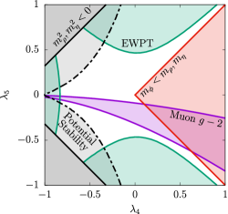
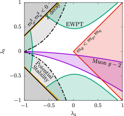
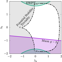
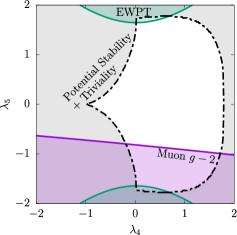
Figure 5: Numerical analysis in ($\lambda_{4}$, $\lambda_{5}$) plane, where the charged scalar mass and Yukawa couplings ($m_{\phi}$, $y_{\mu\tau}$, $y_{\tau\mu}$) are fixed as $(200~{}\mathrm{GeV}$, $0.20$, $0.20$) on top left panel, ($200~{}\mathrm{GeV}$, $0.04$, $1.00$) on top right panel, ($700~{}\mathrm{GeV}$, $0.70$, $0.70$) on bottom left panel, and ($700~{}\mathrm{GeV}$, $0.41$, $1.20$) on bottom right panel, respectively.

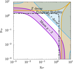
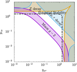
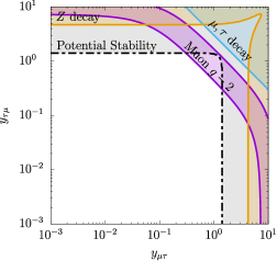
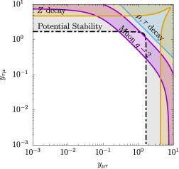
Figure 6: Numerical analysis in ($y_{\mu\tau}$, $y_{\tau\mu}$) plane, where the charged scalar mass and the scalar quartic couplings ($m_{\phi}$, $\lambda_{4}$, $\lambda_{5}$) are fixed as ($200~{}\mathrm{GeV}$, $-0.01$, $-0.20$) on top left panel, ($200~{}\mathrm{GeV}$, $0.30$, $-0.40$) on top right panel, ($700~{}\mathrm{GeV}$, $0.01$, $-1.00$) on bottom left panel and ($700~{}\mathrm{GeV}$, $1.00$, $-1.00$) on bottom right panel, respectively.

We explore parameter space which can explain the discrepancy in the muon $g-2$ while satisfying the relevant constraints. In Fig. 5, we present the numerical analysis in the ($\lambda_{4}$, $\lambda_{5}$) plane for fixed values of charged scalar mass ($m_{\phi}$) and Yukawa couplings ($y_{\mu\tau}$, $y_{\tau\mu}$). In this subsection, we restrict new Yukawa couplings to be real. The upper (lower) two panels show the low (high) mass scenarios with $m_{\phi}=200\,(700)$ GeV. In the left panels, we maximize the new physics contributions to the muon $g-2$, where $y_{\mu\tau}=y_{\tau\mu}$ is assumed, while hierarchical Yukawa couplings are taken in the right panels such that the magnitude of the product $y_{\mu\tau}y_{\tau\mu}$ is retained as same with the left panels so that the parameter space favored by muon $g-2$ does not change. The purple region represents the parameter space which can accommodate the muon magnetic moment anomaly at $2\sigma$ confidence level (CL). In the top panels in Fig. 5, the left-top and left-bottom region colored by gray is forbidden because the mass of the neutral scalars $\rho$ or $\eta$ becomes negative. The green region is ruled out by the electroweak precision tests at $2\sigma$ CL. This constraint becomes stronger for lighter scalar masses. On the other hand, even if the charged scalar mass is relatively light, the constraint can be evaded if $\lambda_{4}\sim\pm\lambda_{5}$, which implies that one of $\rho$ and $\eta$ is nearly degenerate with the charged scalar $\phi^{+}$. The orange region is excluded by the constraint of the lepton universality ($Z$ boson decays). Since the loop corrections to the $Z$ boson decays given by Eq. (42)-(45) are proportional to $|y_{\mu\tau}|^{2}$ or $|y_{\tau\mu}|^{2}$, one can find that the constraint becomes stronger for larger hierarchy between $y_{\mu\tau}$ and $y_{\tau\mu}$ for a fixed $y_{\mu\tau}y_{\tau\mu}$. Note that the loop corrections for the charged lepton currents given by Eq. (29) also have the same dependence on the Yukawa couplings. However, the constraint from muon and tau lepton decays are slightly weaker than the $Z$ boson decays in the above parameter sets. The red region shows the parameter space that the charged scalar $\phi^{+}$ becomes the lightest than the neutral scalars $\rho$ and $\eta$. In this region, since the charged scalar decays dominantly into a pair of a charged lepton and a neutrino, the LHC mass limit ($m_{\phi}\gtrsim 700~{}\mathrm{GeV}$) is applied. The outside of the dot-dashed curve colored by gray is disfavored by the potential stability conditions given by Eq (8) and the triviality. The negative $\lambda_{4}$ region tends to be excluded by the potential stability conditions while the remaining region is bounded by the triviality of the quartic couplings $\lambda_{i}~{}(i=1-5)$. Here, we take $\lambda_{2}=\lambda_{3}=0.5$ at the $Z$ boson mass scale as an initial condition of the renormalization group equation. Note that if smaller couplings $\lambda_{2}$ and $\lambda_{3}$ are assumed, the bound of the potential stability becomes stronger as we expect from Eq. (8).

In Fig. 6, we show the parameter space in the ($y_{\mu\tau}$, $y_{\tau\mu}$) plane by fixing the scalar masses $m_{\rho}$, $m_{\eta}$ and $m_{\phi}$. The positive Yukawa coupling $y_{\mu\tau}$ is chosen without loss of generality. We here concentrate on the case with negative values of $\lambda_{5}$, which is favored by the muon $g-2$ anomaly together with a positive value of $y_{\tau\mu}$. At the same time, we assume a negative $\lambda_{4}+\lambda_{5}$ for $m_{\phi}=200~{}\mathrm{GeV}$. This parameter choice allows the cascade decay of the charged scalar to other scalars, and therefore we can avoid the strong constraint on the charged scalar mass from the LHC slepton search. The purple region can accommodate the muon $g-2$ anomaly at $2\sigma$ CL, while the orange and light blue region are excluded by the lepton universality of the $Z$ boson decays and the charged lepton decays, respectively. The constraint of the electroweak precision tests is satisfied in all the plots, which does not depend on the Yukawa couplings. One can see from Fig. 6 that the constraint of the charged lepton decays (light blue) is always stronger than that of the $Z$ boson decay (orange) when the Yukawa couplings are same order ($y_{\mu\tau}\sim y_{\tau\mu}$). This is due to the the tree level correction given by Eq. (27). In contrast, when the Yukawa couplings are hierarchical, one of the loop corrections for the charged lepton and $Z$ boson decays becomes stronger. The gray region surrounded by the dot-dashed line shows the bounds of the potential stability. In fact, the potential stability bounds are slightly stronger than the triviality bounds. This is because we take the negative quartic couplings $\lambda_{4}$ and $\lambda_{5}$ at the electroweak scale, and the Yukawa couplings involved in the $\beta_{\lambda_{4}}$ and $\beta_{\lambda_{5}}$ make $\lambda_{4}$ and $\lambda_{5}$ further negative at the cut-off scale if the Yukawa couplings are $\mathcal{O}(1)$. As a result, it conflicts with Eq. (8) at the cut-off scale. Note that this bound is relaxed if a smaller cut-off scale $\Lambda$ is assumed.

5 Discussions

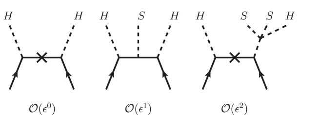
Figure 7: Feynman diagrams for neutrino mass generation through seesaw mechanism under the $Z_{4}$ flavor symmetry.

5.1 Neutrino Mass Generation Sector

As we mentioned in the beginning, the $Z_{4}$ flavor symmetry in our minimal model must be broken in order to fit the observed data of neutrino masses and mixings. As a simple example for neutrino mass generation, we here consider the type-I seesaw mechanism. A SM singlet scalar $S$ with $Z_{4}$ charge $\omega$ and a three generation of right-handed neutrinos $(N_{1R},N_{2R},N_{3R})$ with $(1,\omega,\underline{\omega})$ are introduced to the model. The Lagrangian for the neutrino mass generation sector is

$$-{\mathcal{L}}_{N} =+\frac{1}{2}\begin{pmatrix}\overline{N_{1R}^{c}}&\overline{N_{2R}^{c}}&\overline{N_{3R}^{c}}\end{pmatrix}\begin{pmatrix}M_{1}&y_{12}S^{*}&y_{13}S\\ y_{12}S^{*}&&M_{23}\\ y_{13}S&M_{23}&\end{pmatrix}\begin{pmatrix}N_{1R}\\ N_{2R}\\ N_{3R}\end{pmatrix}$$

$$\qquad+\begin{pmatrix}\overline{L_{e}}&\overline{L_{\mu}}&\overline{L_{\tau}}\end{pmatrix}\begin{pmatrix}y_{e1}\tilde{H}&&\\ &y_{\mu 2}\tilde{H}&y_{\mu 3}\tilde{\Phi}\\ &y_{\tau 2}\tilde{\Phi}&y_{\tau 3}\tilde{H}\end{pmatrix}\begin{pmatrix}N_{1R}\\ N_{2R}\\ N_{3R}\end{pmatrix}+\text{H.c.}$$ (50)

where $\tilde{X}=i\sigma_{2}X^{*}~{}(X=H,\Phi)$. The singlet $S$ is assumed to have a VEV $\epsilon\langle S\rangle$, which breaks the $Z_{4}$ symmetry, where $\epsilon$ is introduced to count the order of singlet VEVs. At leading order, ${\mathcal{O}}(\epsilon^{0})$, the (symmetric) neutrino mass matrix has non-zero values only in $(1,1)$ and $(2,3)$ elements (see also Fig. 7). At this order, due to the vanishing $(2,2)$ and $(3,3)$ elements, a large $\theta_{23}$ mixing is naturally obtained in this model. At the next leading order, ${\mathcal{O}}(\epsilon^{1})$, the matrix takes the two zero minor structure [18, 32]. This form of the neutrino mass matrix confronts a severe constraint on the sum of neutrino masses from cosmological observation [33]. In our model, a quartic term, $\kappa\,S^{2}H^{{\dagger}}\Phi$, is allowed by the $Z_{4}$ flavor symmetry. Through this coupling, a small VEV for $\Phi$, i.e., $\langle\Phi\rangle\sim\kappa\,\epsilon^{2}(\langle S\rangle^{2}/M_{\phi}^{2})v$ is induced from the singlet VEV. As a result, at ${\mathcal{O}}(\epsilon^{2})$ we have additional contributions to the mass matrix. Then, the total structure of the neutrino mass matrix is

$$M_{\nu}\propto\begin{pmatrix}{\mathcal{O}}(\epsilon^{0})&{\mathcal{O}}(\epsilon)&{\mathcal{O}}(\epsilon)\\ {\mathcal{O}}(\epsilon)&{\mathcal{O}}(\kappa\,\epsilon^{2})&{\mathcal{O}}(\epsilon^{0})\\ {\mathcal{O}}(\epsilon)&{\mathcal{O}}(\epsilon^{0})&{\mathcal{O}}(\kappa\,\epsilon^{2})\end{pmatrix}.$$ (51)

Therefore, in the present model, the constraints from neutrino data are relatively relaxed as compared with the minimal gauged $U(1)_{{\mathbf{L}}_{\mu}-{\mathbf{L}}_{\tau}}$ model.

5.2 Collider Signature

In the previous section, we have taken into account the direct collider search constraint of charged scalars ($m_{\phi}\gtrsim 700~{}\mathrm{GeV}$). This bound will be improved further at the future LHC running by the same search mode. In our model, the neutral scalars $(\rho,\eta)$ can be lighter than the charged scalar. Such light scalars can be produced at the LHC, and give interesting distinctive signals. Because of the flavor charge conservation in the $Z_{4}$ symmetric limit, they are produced in a pair $q\bar{q}\,(e^{+}e^{-})\to\rho\,\eta$ at hadron (lepton) colliders and their primary decay modes are $\mu\tau$ pairs. So far no dedicated search has been performed, and it was shown in the Type-X THDM that $2\mu 2\tau$ final states can be approximately reconstructed even at the hadron collider [34]. Application of this analysis to our model seems to be easy. Firstly, there is no suppression of the signal events by their branching ratio. Secondly, thanks to the collinear approximation of tau leptons, the LFV invariant mass $M_{\mu\tau}$ is fully reconstructable. Then, $M_{\mu\tau}$ is used for a very good discriminant against background events. The study for the discovery potential of $(\rho,\eta)$ is beyond the scope of this paper, and we leave it for the future.

5.3 Indirect Signals

5.3.1 Muon Electric Dipole Moment

If the new Yukawa couplings $y_{\mu\tau}$, $y_{\tau\mu}$ are complex, electric dipole moment (EDM) of muon is induced by the same diagram for muon anomalous magnetic moment in Fig. 2, which is computed as

$$\frac{d_{\mu}}{e}=\frac{\mathrm{Im}\left(y_{\mu\tau}y_{\tau\mu}\right)}{2(4\pi)^{2}}\left[\frac{m_{\tau}}{m_{\rho}^{2}}I_{2}\left(\frac{m_{\mu}^{2}}{m_{\rho}^{2}},\frac{m_{\tau}^{2}}{m_{\rho}^{2}}\right)-\frac{m_{\tau}}{m_{\eta}^{2}}I_{2}\left(\frac{m_{\mu}^{2}}{m_{\eta}^{2}},\frac{m_{\tau}^{2}}{m_{\eta}^{2}}\right)\right].$$ (52)

Similar to the case of muon magnetic moment, Eq. (52) has a potentially large contribution from the chirality flipping effect.

The current experimental bound for muon EDM is given by the Muon $g-2$ Collaboration (BNL) as [35]

$$\frac{|d_{\mu}|}{e}<1.9\times 10^{-19}~{}\mathrm{cm}.$$ (53)

In addition to the current bound, factor $10$ improvement is expected by the future FNAL E989 experiment [36], and the future sensitivity of the J-PARC $g-2$/EDM Collaboration is roughly $|d_{\mu}|/e\sim 10^{-21}~{}\mathrm{cm}$ [37].

In the left panel of Fig. 8, we give a contour plot of the muon EDM predictions in the ($m_{\rho}$, $m_{\eta}$) plane where we assume $\mathrm{Im}\left(y_{\mu\tau}y_{\tau\mu}\right)=1$. The yellow region is already excluded by the current muon EDM limit. We see that the current muon EDM limit does not exclude the model without requiring the tuning in the imaginary part of the Yukawa couplings. The solid purple and dashed green lines are the future sensitivities of the FNAL E989 and J-PARC $g-2$/EDM, respectively. Although the constraint of the current bound is not so strong, the future experiments can explore parameter space furthermore.

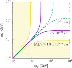
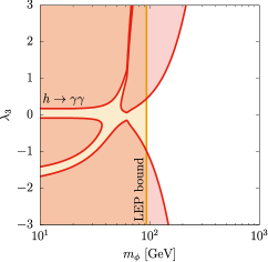
Figure 8: Left: Contours of muon EDM $|d_{\mu}|/e$ where $\mathrm{Im}\left(y_{\mu\tau}y_{\tau\mu}\right)=1$. The yellow region is excluded by the Muon $g-2$ Collaboration, and the solid purple and dashed green lines are the future prospect of EDM experimental reach. Right: Parameter space excluded by $h\to\gamma\gamma$ signal strength (red) and the LEP bound (orange) in ($m_{\phi}$, $\lambda_{3}$) plane.

5.3.2 $h\to\gamma\gamma$

The additional contribution to $h\to\gamma\gamma$ can appear through the charged scalar loop. The decay amplitude including the SM contribution is computed as [38, 39]

$$i\mathcal{M}_{h\to\gamma\gamma}=\frac{igm_{W}\alpha_{\mathrm{em}}}{(2\pi)\tau_{W}}\epsilon_{\mu}^{*}\epsilon_{\nu}^{*}g^{\mu\nu}\left[F_{1}\left(\tau_{W}\right)+\sum_{f}N_{c}Q_{f}^{2}F_{1/2}\left(\tau_{f}\right)+\frac{\lambda_{3}v^{2}}{2m_{\phi}^{2}}F_{0}\left(\tau_{\phi}\right)\right],$$ (54)

where $\tau_{i}\equiv 4m_{i}^{2}/m_{h}^{2}$, $N_{c}=1,3$ is color factor, $Q_{f}$ is the electric charge of the SM fermions, $\epsilon_{\mu/\nu}$ is the photon polarization vector, and the loop functions $F_{1}(\tau)$, $F_{1/2}(\tau)$ and $F_{0}(\tau)$ are given by

$$F_{1}(\tau) =2+3\tau+3\tau\left(2-\tau\right)f(\tau),$$ (55)

$$F_{1/2}(\tau) =-2\tau\Bigl{(}1+(1-\tau)f(\tau)\Bigr{)},$$ (56)

$$F_{0}(\tau) =\tau\Bigl{(}1-\tau f(\tau)\Bigr{)},$$ (57)

with

$$f(\tau)=\left\{\begin{array}[]{cc}\displaystyle\mathrm{arcsin}^{2}\left(\frac{1}{\sqrt{\tau}}\right)&\text{for}\quad\tau>1\\ \displaystyle-\frac{1}{4}\left[\log\left(\frac{1+\sqrt{1-\tau}}{1-\sqrt{1-\tau}}\right)-i\pi\right]^{2}&\text{for}\quad\tau<1\end{array}\right..$$ (60)

The last term in Eq. (54) corresponds to the new contribution which is controlled by the quartic coupling $\lambda_{3}$ in the scalar potential. Then, the partial decay width is calculated as

$$\Gamma_{h\to\gamma\gamma}=\frac{G_{\!F}\alpha_{\mathrm{em}}^{2}m_{h}^{3}}{128\sqrt{2}\pi^{3}}\left|F_{1}\left(\tau_{W}\right)+\sum_{f}N_{c}Q_{f}^{2}F_{1/2}\left(\tau_{f}\right)+\frac{\lambda_{3}v^{2}}{2m_{\phi}^{2}}F_{0}\left(\tau_{\phi}\right)\right|^{2}.$$ (61)

The signal strength for $h\to\gamma\gamma$ defined by the ratio of the observed Higgs boson decay to the SM prediction has been reported as $\mu=0.99_{-0.14}^{+0.15}$ by the ATLAS Collaboration [40], and $1.18_{-0.14}^{+0.17}$ by the CMS Collaboration [41]. The signal strength deviates from unity if non-zero value of the quartic coupling $\lambda_{3}$ exists. The constrained parameter space in the ($m_{\phi}$, $\lambda_{3}$) plane is shown in the right panel of Fig. 8, where the red region is excluded by the PDG data $\mu=1.16\pm 0.18$ at $2\sigma$ CL [1], and the orange region is excluded by the LEP limit $m_{\phi}\lesssim 93.5~{}\mathrm{GeV}$. One can see that the parameter space with $|\lambda_{3}|=\mathcal{O}(1)$ is ruled out if $100~{}\mathrm{GeV}\lesssim m_{\phi}\lesssim 200~{}\mathrm{GeV}$. There is no substantial constraint if $m_{\phi}\gtrsim 200~{}\mathrm{GeV}$.

6 Summary and Conclusions

We have studied models based on leptonic flavor symmetries, which can accommodate the long-standing muon $g-2$ anomaly. The minimal model is based on a $Z_{4}$ lepton flavor symmetry, and includes an inert doublet scalar charged under the flavor symmetry. Large muon anomalous magnetic moment is realized by the chirality enhancement with the factor $m_{\tau}/m_{\mu}\approx 17$ in this model. We have also analytically formulated the constraints from the electroweak precision tests and lepton universality. Taking into account all these constraints, allowed parameter space is explored numerically. For the electroweak precision tests, it has been found that the constraint can easily be evaded if the quartic couplings $\lambda_{4}$ and $\lambda_{5}$ are relatively small or the relation $\lambda_{5}\sim\pm\lambda_{4}$ is satisfied, which corresponds to one of neutral scalars $\rho$ and $\eta$ is nearly degenerate with the charged scalar $\phi^{+}$. For lepton universality, we have computed tree and one-loop corrections of heavier charged lepton decays, and one-loop correction for $Z$ boson decay. We have found that the tree level correction becomes dominant when the Yukawa couplings are comparable ($y_{\mu\tau}\sim y_{\tau\mu}$) while the loop correction becomes important for hierarchical Yukawa couplings. In addition, we have numerically examined the potential stability conditions and triviality bounds assuming the cut-off scale of the model, $\Lambda=100~{}\mathrm{TeV}$. We have successfully found that the parameter region where the discrepancy in the muon $g-2$ is explained at $2\sigma$ level while satisfying all relevant constraints. As further perspective of the minimal $Z_{4}$ model, neutrino mass generation with Type-I seesaw mechanism, discriminative collider signatures, indirect signals from muon EDM and Higgs decay width into $\gamma\gamma$ have also been discussed. We have also found that some parameter space can be explored by the future EDM experiments if rather large CP phase exists in the Yukawa couplings. The signal strength of the Higgs decay width into $\gamma\gamma$ is influenced by the new contribution if the charged scalar mass is less than $200~{}\mathrm{GeV}$.

Appendix A

We list the $\beta$ functions for the gauge couplings, quartic couplings and Yukawa couplings at one loop level, which have been used to derive the triviality bound. We have used the public package SARAH [42, 43] to obtain the following analytic expressions. Note that the effect of the charged lepton and quark Yukawa couplings are neglected except for the top Yukawa coupling.

$\beta$ functions for gauge couplings:

$$\beta_{g^{\prime}} =7{g^{\prime}}^{3},$$ (62)

$$\beta_{g} =-3g^{3},$$ (63)

$$\beta_{g_{c}} =-7g_{c}^{3}.$$ (64)

$\beta$ functions for quartic couplings:

$$\beta_{\lambda_{1}} =\frac{3}{8}{g^{\prime}}^{4}+\frac{3}{4}{g^{\prime}}^{2}g^{2}+\frac{9}{8}g^{4}-3\lambda_{1}\left({g^{\prime}}^{2}+3g^{2}\right)+24\lambda_{1}^{2}+2\lambda_{3}^{2}+2\lambda_{3}\lambda_{4}+\lambda_{4}^{2}+\lambda_{5}^{2}$$

$$~{}~{}~{}+12\lambda_{1}y_{t}^{2}-6y_{t}^{4},$$ (65)

$$\beta_{\lambda_{2}} =\frac{3}{8}{g^{\prime}}^{4}+\frac{3}{4}{g^{\prime}}^{2}g^{2}+\frac{9}{8}g^{4}-3\lambda_{2}\left({g^{\prime}}^{2}+3g^{2}\right)+24\lambda_{2}^{2}+2\lambda_{3}^{2}+2\lambda_{3}\lambda_{4}+\lambda_{4}^{2}+\lambda_{5}^{2}$$

$$~{}~{}~{}+4\lambda_{2}\left(|y_{\mu\tau}|^{2}+|y_{\tau\mu}|^{2}\right)-2\left(|y_{\mu\tau}|^{4}+|y_{\tau\mu}|^{4}\right),$$ (66)

$$\beta_{\lambda_{3}} =\frac{3}{4}{g^{\prime}}^{4}+\frac{3}{2}{g^{\prime}}^{2}g^{2}+\frac{9}{4}g^{4}-3\lambda_{3}\left({g^{\prime}}^{2}+3g^{2}\right)+4\left(\lambda_{1}+\lambda_{2}\right)\left(3\lambda_{3}+\lambda_{4}\right)$$

$$~{}~{}~{}+4\lambda_{3}^{2}+2\lambda_{4}^{2}+10\lambda_{5}^{2}+2\lambda_{3}\left(|y_{\mu\tau}|^{2}+|y_{\tau\mu}|^{2}+3y_{t}^{2}\right),$$ (67)

$$\beta_{\lambda_{4}} =-3{g^{\prime}}^{2}g^{2}-3\lambda_{4}\left({g^{\prime}}^{2}+3g^{2}\right)+4\left(\lambda_{1}+\lambda_{2}+2\lambda_{3}+\lambda_{4}\right)\lambda_{4}-8\lambda_{5}^{2}$$

$$~{}~{}~{}+2\lambda_{4}\left(|y_{\mu\tau}|^{2}+|y_{\tau\mu}|^{2}+3y_{t}^{2}\right),$$ (68)

$$\beta_{\lambda_{5}} =-3\left({g^{\prime}}^{2}+3g^{2}\right)\lambda_{5}+4\left(\lambda_{1}+\lambda_{2}+2\lambda_{3}-\lambda_{4}\right)\lambda_{5}+2\lambda_{5}\left(|y_{\mu\tau}|^{2}+|y_{\tau\mu}|^{2}+3y_{t}^{2}\right).$$ (69)

$\beta$ functions for Yukawa couplings:

$$\beta_{y_{\mu\tau}} =\left[\frac{5}{2}|y_{\mu\tau}|^{2}+|y_{\tau\mu}|^{2}-\frac{9}{4}\left(\frac{5}{3}{g^{\prime}}^{2}+g^{2}\right)\right]y_{\mu\tau},$$ (70)

$$\beta_{y_{\tau\mu}} =\left[|y_{\mu\tau}|^{2}+\frac{5}{2}|y_{\tau\mu}|^{2}-\frac{9}{4}\left(\frac{5}{3}{g^{\prime}}^{2}+g^{2}\right)\right]y_{\tau\mu},$$ (71)

$$\beta_{y_{t}} =\left[-\frac{17}{12}{g^{\prime}}^{2}-\frac{9}{4}g^{2}-8g_{c}^{2}+\frac{9}{2}y_{t}^{2}\right]y_{t}.$$ (72)

References

- [1] M. Tanabashi et al. [Particle Data Group], Phys. Rev. D 98, no. 3, 030001 (2018).
- [2] A. Keshavarzi, D. Nomura and T. Teubner, Phys. Rev. D 97, no. 11, 114025 (2018) [arXiv:1802.02995 [hep-ph]].
- [3] J. Prades, E. de Rafael and A. Vainshtein, Adv. Ser. Direct. High Energy Phys. 20, 303 (2009) [arXiv:0901.0306 [hep-ph]].
- [4] A. Chapelain [Muon g-2 Collaboration], EPJ Web Conf. 137, 08001 (2017) [arXiv:1701.02807 [physics.ins-det]].
- [5] T. Abe, R. Sato and K. Yagyu, JHEP 1707, 012 (2017) [arXiv:1705.01469 [hep-ph]].
- [6] E. J. Chun and J. Kim, JHEP 1607, 110 (2016) [arXiv:1605.06298 [hep-ph]].
- [7] T. Abe, R. Sato and K. Yagyu, JHEP 1507, 064 (2015) [arXiv:1504.07059 [hep-ph]].
- [8] A. Crivellin, D. Müller and C. Wiegand, arXiv:1903.10440 [hep-ph].
- [9] Y. Omura, E. Senaha and K. Tobe, JHEP 1505, 028 (2015) [arXiv:1502.07824 [hep-ph]].
- [10] Y. Omura, E. Senaha and K. Tobe, Phys. Rev. D 94, no. 5, 055019 (2016) [arXiv:1511.08880 [hep-ph]].
- [11] S. Baek, N. G. Deshpande, X. G. He and P. Ko, Phys. Rev. D 64, 055006 (2001) [hep-ph/0104141].
- [12] E. Ma, D. P. Roy and S. Roy, Phys. Lett. B 525, 101 (2002) [hep-ph/0110146].
- [13] M. Endo, K. Hamaguchi and G. Mishima, Phys. Rev. D 86, 095029 (2012) [arXiv:1209.2558 [hep-ph]].
- [14] M. Endo, K. Hamaguchi, S. Iwamoto and T. Yoshinaga, JHEP 1401, 123 (2014) [arXiv:1303.4256 [hep-ph]].
- [15] W. J. Marciano, A. Masiero, P. Paradisi and M. Passera, Phys. Rev. D 94, no. 11, 115033 (2016) [arXiv:1607.01022 [hep-ph]].
- [16] S. Bar-Shalom, S. Nandi and A. Soni, Phys. Lett. B 709, 207 (2012) [arXiv:1112.3661 [hep-ph]].
- [17] C. W. Chiang and K. Tsumura, JHEP 1805, 069 (2018) [arXiv:1712.00574 [hep-ph]].
- [18] K. Asai, K. Hamaguchi and N. Nagata, Eur. Phys. J. C 77, no. 11, 763 (2017) [arXiv:1705.00419 [hep-ph]].
- [19] N. G. Deshpande and E. Ma, Phys. Rev. D 18, 2574 (1978).
- [20] T. Hambye, F.-S. Ling, L. Lopez Honorez and J. Rocher, JHEP 0907, 090 (2009) Erratum: [JHEP 1005, 066 (2010)] [arXiv:0903.4010 [hep-ph]].
- [21] M. E. Peskin and T. Takeuchi, Phys. Rev. D 46, 381 (1992).
- [22] R. Barbieri, L. J. Hall and V. S. Rychkov, Phys. Rev. D 74, 015007 (2006) [hep-ph/0603188].
- [23] M. E. Peskin and J. D. Wells, Phys. Rev. D 64, 093003 (2001) [hep-ph/0101342].
- [24] S. Kanemura, Y. Okada, H. Taniguchi and K. Tsumura, Phys. Lett. B 704, 303 (2011) [arXiv:1108.3297 [hep-ph]].
- [25] M. Baak et al. [Gfitter Group], Eur. Phys. J. C 74, 3046 (2014) [arXiv:1407.3792 [hep-ph]].
- [26] W. J. Marciano and A. Sirlin, Phys. Rev. Lett. 61, 1815 (1988).
- [27] Y. Amhis et al. [Heavy Flavor Averaging Group (HFAG)], arXiv:1412.7515 [hep-ex].
- [28] S. Schael et al. [ALEPH and DELPHI and L3 and OPAL and SLD Collaborations and LEP Electroweak Working Group and SLD Electroweak Group and SLD Heavy Flavour Group], Phys. Rept. 427, 257 (2006) [hep-ex/0509008].
- [29] G. Abbiendi et al. [ALEPH and DELPHI and L3 and OPAL and LEP Collaborations], Eur. Phys. J. C 73, 2463 (2013) [arXiv:1301.6065 [hep-ex]].
- [30] M. Aaboud et al. [ATLAS Collaboration], Eur. Phys. J. C 78, no. 12, 995 (2018) [arXiv:1803.02762 [hep-ex]].
- [31] The ATLAS collaboration [ATLAS Collaboration], ATLAS-CONF-2019-008.
- [32] K. Asai, K. Hamaguchi, N. Nagata, S. Y. Tseng and K. Tsumura, Phys. Rev. D 99, no. 5, 055029 (2019) [arXiv:1811.07571 [hep-ph]].
- [33] N. Aghanim et al. [Planck Collaboration], arXiv:1807.06209 [astro-ph.CO].
- [34] S. Kanemura, K. Tsumura and H. Yokoya, Phys. Rev. D 85, 095001 (2012) [arXiv:1111.6089 [hep-ph]].
- [35] G. W. Bennett et al. [Muon (g-2) Collaboration], Phys. Rev. D 80, 052008 (2009) [arXiv:0811.1207 [hep-ex]].
- [36] J. Price, talk at “Workshop on future muon EDM searches at Fermilab and worldwide”, https://indico.fnal.gov/event/18239/.
- [37] N. Saito [J-PARC g-’2/EDM Collaboration], AIP Conf. Proc. 1467, 45 (2012).
- [38] A. Djouadi, Phys. Rept. 457, 1 (2008) [hep-ph/0503172].
- [39] B. Swiezewska and M. Krawczyk, Phys. Rev. D 88, no. 3, 035019 (2013) [arXiv:1212.4100 [hep-ph]].
- [40] M. Aaboud et al. [ATLAS Collaboration], Phys. Rev. D 98, 052005 (2018) [arXiv:1802.04146 [hep-ex]].
- [41] A. M. Sirunyan et al. [CMS Collaboration], JHEP 1811, 185 (2018) [arXiv:1804.02716 [hep-ex]].
- [42] F. Staub, Comput. Phys. Commun. 182, 808 (2011) [arXiv:1002.0840 [hep-ph]].
- [43] F. Staub, Comput. Phys. Commun. 185, 1773 (2014) [arXiv:1309.7223 [hep-ph]].