ViDeNN: Deep Blind Video Denoising

Abstract

We propose ViDeNN: a CNN for Video Denoising without prior knowledge on the noise distribution (blind denoising). The CNN architecture uses a combination of spatial and temporal filtering, learning to spatially denoise the frames first and at the same time how to combine their temporal information, handling objects motion, brightness changes, low-light conditions and temporal inconsistencies. We demonstrate the importance of the data used for CNNs training, creating for this purpose a specific dataset for low-light conditions. We test ViDeNN on common benchmarks and on self-collected data, achieving good results comparable with the state-of-the-art.

1 Introduction

Image and video denoising aims to obtain the original signal $X$ from available noisy observations $Y$. Noise influences the perceived visual quality, but also segmentation [1] and compression [2] making denoising an important step. With $X$ as the original signal, $N$ as the noise and $Y$ as the available noisy observation, the noise degradation model can be described as $Y=X+N$, for an additive type of noise. In low-light conditions, noise is signal dependent and more sensitive in dark regions, modeled as $Y=H(X)+N$, with $H$ as the degradation function.

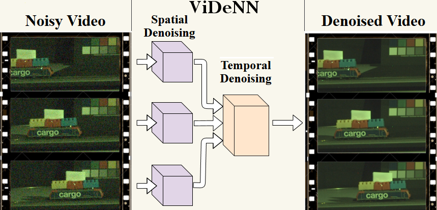
Figure 1: ViDeNN approach to Video Denoising: combining two networks performing first Single Frame Spatial Denoising and subsequently Temporal Denoising over a window of three frames, all in a single feed-forward process.

Imaging noise is due to thermal effects, sensor imperfections or low-light. Hand tuning multiple filter parameters is fundamental to optimize quality and bandwidth of new cameras for each gain level, taking much time and effort. Here, we automate the denoising procedure with a CNN for flexible and efficient video denoising, capable to blindly remove noise. Having a noise removal algorithm working in “blind” conditions is essential in a real-world scenario where color and light conditions can change suddenly, producing a different noise distribution for each frame.

Solutions based on statistical models include Markov Random Field models [3], gradient models [4], sparse models [5] and Nonlocal Self-Similarity (NSS) currently used in state-of-the-art techniques such as BM3D [6], LSSC [7], NCSR [8] and WNNM [9]. Even though they achieve respectable denoising performance, most of those algorithms have some drawbacks. Firstly, they are generally designed to tackle specific noise models and levels, limiting their usage in blind denoising. Secondly, they involve time-consuming hand-tuned optimization procedures.

Much work has been done on image denoising while few algorithms have been specifically designed for videos. The key assumption for video denoising is that video frames are strongly correlated. The most basic video denoising technique consists of the temporal average over various subsequent frames. While giving excellent results for steady scenes, it blurs motion, causing artifacts. The VBM4D method [10] is the state-of-the-art in video denoising. It extends BM3D [6] single image denoising by the search of similar patches, not only in spatial but also in temporal domain. Searching for similar patches in more frames drastically increases the processing time.

In this paper we propose ViDeNN, illustrated in Fig 1: a convolutional neural network for blind video denoising, capable to denoise videos without prior knowledge over the noise model and the video content. For comparison, experiments have been run on publicly available and on self captured videos. The videos, the low-light dataset and the code will be published on the project’s GitHub page.
The main contributions of our work are: (i) a novel CNN architecture capable to blind denoise videos, combining spatial and temporal information of multiple frames with one single feed-forward process; (ii) Flexibility tests on Additive White Gaussian Noise and real data in low-light condition; (iii) Robustness to motion in challenging situations; (iv) A new low-light dataset for a specific Bosch security camera, with sample pairs of noise-free and noisy images.

2 Related Work

CNNs for Image Denoising. From the 2008 CNN image denoising work of Jain and Seung [11] there have been huge improvements thanks to more computational power and high quality datasets. In 2012, Burger et al. [12] showed how even a simple Multi Layer Perceptron can obtain comparable results with BM3D [6], even though a huge dataset was required for training [13]. Recently, in 2016, Zhang et al. [14] used residual learning and Batch Normalization [15] for image denoising in their DnCNN architecture. With its simple yet effective architecture, it has shown to be flexible for tasks as blind Gaussian denoising, JPEG deblocking and image inpainting. FFDNet [16] extends DnCNN by handling an extended range of noise levels and has the ability to remove spatially variant noise. Ulyanov et al. [17] showed how, with their Deep Prior, they can enhance a given image with no prior training data other than the image itself, which can be seen as a ”blind” denoising. There have been also some works on CNNs directly inspired by BM3D such as [18, 19]. In [20], Ying et al. propose a deep persistent memory network called MemNet that obtains valid results, introducing a memory block, motivated by the fact that human thoughts are persistent. However, the network structure remains complex and not easily reproducible. A U-Net variant has been successfully used for image denoising in the work of Xiao-Jiao et al. [21] and in the most recent work on image denoising of Guo et al. [22] called CBDNet. With their novel approach, CBDNet reaches extraordinarily results in real world blind image denoising. The recently proposed Noise2Noise [23] model is based on an encoder-decoder structure, obtains almost the same result using only noisy images for training, instead of clean-noisy pairs, which is particularly useful for cases where the ground truth is not available.

Video and Deep Neural Networks. Video denoising using deep learning is still an under-explored research area. The seminal work of Xinyuan et al. [24], is currently the only one using neural networks (Recurrent Neural Networks) to address video denoising. We differ by addressing color video denoising, and offer comparable results to the state-of-art. Other video-based tasks addressed using CNNs include Video Frame Enhancement, Interpolation, Deblurring and Super-Resolution, where the key component is how to handle motion and temporal changes. For frame interpolation, Niklaus et al. [25] use a pre-computed optical flow to feed motion information to a frame interpolation CNN. Meyer et al. [26] use instead phase based features to describe motion. Caballero et al. [27] developed a network which estimate the motion by itself for video super resolution. Similarly, in Multi Frame Quality Enhancement (MFQE), Yang et al. [28] use a Motion Compensation Network and a Quality Enhancement Network, considering three non-consecutive frames for H265 compressed videos. Specifically for video deblurring, Su et al. [29] developed a network called DeBlurNet: a U-Net CNN which takes three frames stacked together as input. Similarly, we also use three stacked frames in our ViDeNN. Additionally, we have also investigated variations in the number of input frames.

Real World Datasets. An image or video denoising algorithm, has to be effective on real world data to be successful. However, it is hard to obtain the ground truth for real pictures, since perfect sensors and channels do not exist. In 2014, Anaya and Barbu, created a dataset for low-light conditions called RENOIR [30]: they use different exposure times and ISO levels to get noisy and clean images of the same static scene. Similarly, in 2017, Plotz and Roth created a dataset called DND [31]. In this case, only the noisy samples have been released, whereas the noise free ones are kept undisclosed for benchmarking purposes. Recently, two other related papers have been published. The first, written by Abdelhamed et al. [32] concerns the creation of a smartphone image dataset of noisy and clean images, which at the time of writing is not yet publicly available. The second, written by Chen et al. [33], presents a new CNN based algorithm capable to enhance the quality of low-light raw images. They created a dedicated dataset of two camera types similarly to [30].

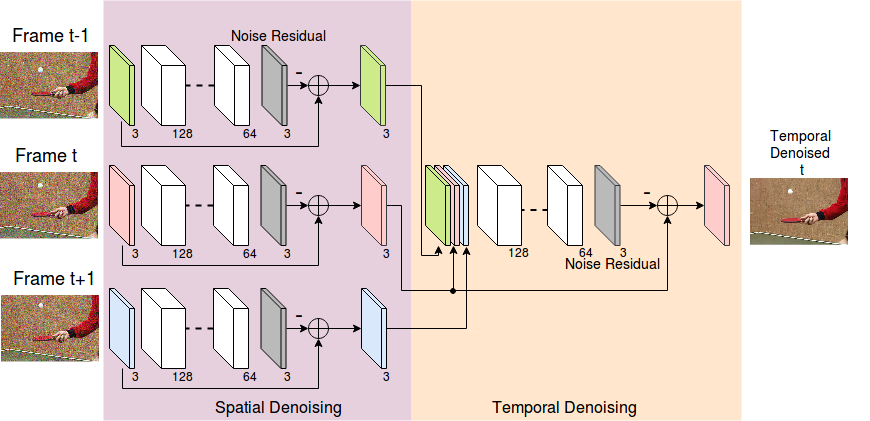
Figure 2: The architecture of the proposed ViDeNN network. Every frame will go through a spatial denoising CNN. The temporal CNN takes as input three spatially denoised frames and outputs the final estimate of the central frame. Both CNNs estimate first the noise residual, i.e. the unwanted values noise adds to an image, and then subtracts them from the noisy input ($\oplus$ means addition of the two signals, and ”-” the negation). ViDeNN is composed only by Convolutional Layers. The number of feature maps is written at the bottom of each layer.

3 ViDeNN: Video DeNoising Net

ViDeNN has two subnetworks: Spatial and temporal denoising CNN, as illustrated in Fig 2.

3.1 Spatial Denoising CNN

For spatial denoising we build on [14], which showed great flexibility tackling multiple degradation types at the same time, and experimented with the same architecture for blind spatial denoising. It is shown, that this architecture can achieve state-of-art results for Gaussian denoising. A first layer of depth 128 helps when the network has to handle different noise models at the same time. The network depth is set to 20 and Batch Normalization (BN) [15] is used. The activation function is ReLU (Rectified Linear Unit). We also investigated the use of Leaky ReLU as activation function, which can be more effective [34], without improvement over ReLU. Comparison results are provided in the supplementary material. Our Spatial-CNN uses Residual Learning, which has been firstly introduced in [14] to tackle image denoising. Instead of forcing the network to output directly the denoised frame, the residual architecture predicts the residual image, which consist in the difference between the original clean image and the noisy observation. The loss function $L$ is the L2-norm, also known as least squares error (LSE) and is the sum of the square of the differences $S$ between the target value $Y$ and the estimated values $Y_{est}$. In this case the difference $S$ represents the noise residual image estimated by the Spatial-CNN, and is given by $L=\sum\limits_{x}\sum\limits_{y}\Big{(}\underbrace{Y(x,y)-Y_{est}(x,y)}_{\text{Noise Residual}}\Big{)}^{2}$.

3.1.1 A Realistic Noise Model

The denoising performance of a spatial denoising CNN depends greatly on the training data. Real noise distribution differs from Gaussian, since it is not purely additive but it contains a signal dependent part. For this reason, CNN models trained only on Additive White Gaussian Noise (AWGN) fail to denoise real world images [22]. Our goal is to achieve a good balance between performance and flexibility, training a single network for multiple noise models. As shown in Table 1, our Spatial-CNN can handle blind Gaussian denoising: we will further investigate its generalization capabilities, introducing a signal dependent noise model. This specific noise model, in equation 1, is composed by two main contributions, the Photon Shot Noise (PSN) and the Read Noise. The PSN is the main noise source in low-light condition, where $N_{sat}$ accounts the saturation number of electrons. The Read Noise is mainly due to the quantization process in the Analog to Digital Converter (ADC), used to transform the analog light signal into a digital image. $CT1_{n}$ represents the normalized value of the noise contribution due to the Analog Gain, whereas $CT2_{n}$ represents the additive normalized part. The realistic noise model is

$$M=\sqrt[]{\underbrace{\frac{Ag*Dg}{N_{sat}*s}}_{\text{PSN}}+\underbrace{Dg^{2}*(Ag*CT1_{n}+CT2_{n})^{2}}_{\text{Read Noise}}},$$ (1)

$$\text{Noisy Image}=s+\mathcal{N}(0,1)*M(s),$$ (2)

where the relevant terms for the considered Sony sensor are: $Ag$ (Analog Gain), in range [0,64], $Dg$ (Digital Gain), in range [0,32] and $s$, the image that will be degraded. The remaining values are $CT1_{n}$=$1.25^{-4}$, $CT2_{n}$=$1.11^{-4}$ and $N_{sat}$=$7489$. The noisy image is generated by multiplying observations of a normal distribution $\mathcal{N}(0,1)$ with the same shape of the reference image $s$, with the Noise Model $M$ in equation 2. In Figure 3 we illustrate that AWGN-based algorithms such as CBM3D and DnCNN do not generalize to realistic noise. CBM3D, in its blind version, i.e. with the supposed AWGN standard deviation $\sigma$ set to 50, over-smooths the image, getting a low SSIM (Structural Similarity, the higher the better) score, whereas DnCNN preserves more structure. Our result shows that, to better denoise real world images, a realistic noise model has to be used for the training set.

(a)
Noisy frame
(18.54/0.5225)

(b) CBM3D[35]
(29.26/0.9194)

(c) DnCNNB[14]
(28.72/0.9355)

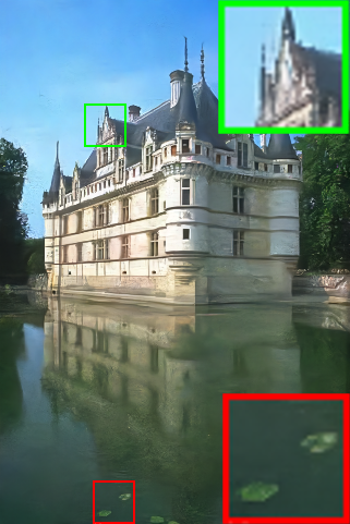
(d)
Our result
(30.37/0.9361)

Figure 3: Comparison of spatial denoising of an image from the CBSD68 dataset corrupted with 1, with Ag=64 and Dg=4. AWGN based method as CBM3D and DnCNN does not achieve optimal result. The first blurs excessively the image. Using the proper noise model for training leads to a better result. (PSNR [dB]/SSIM)

3.2 Temp3-CNN: Temporal Denoising CNN

The temporal denoising part of ViDeNN is similar in structure to the spatial one, having the same number of layers and feature maps. However, it stacks frames together as input. Following other work [27, 28, 29] we stack 3 frames, which is efficient, while our preliminary results show no improvements for stacking more than 3 frames. Considering a frame with dimensions $w{\times}h{\times}c$, the new input will have dimension of $w{\times}h{\times}3c$. Similar to the Spatial-CNN, the temporal denoising also uses residual learning and will estimate the noise residual image of the central input frame, combining the information of other frames allowing it to learn temporal inconsistencies.

4 Experiments

In this section we present the dataset creation and the training/validation, performing insightful experiments.

4.1 Low-Light Dataset Creation

An image denoising dataset has pairs of clean and noisy images. For realistic low-light conditions, creating pairs of noisy and clean images is challenging and the publicly available data is scarce. We used Renoir [30] and our self-collected dataset. Renoir [30] proposes to use two different ISO values and exposure times to get reference and distorted images, demanding many camera settings and parameters. We use a simpler process: grabbing many noisy images of a static scene and then simply averaging to get an estimated ground truth. We used a Bosch Autodome IP 5000 IR, a security camera capable to record raw images, i.e. without any type of processing. The setting involved a static scene and a light source with color temperature $3460K$, which has variable intensity between 0 and 255. We varied the light intensity in 12 steps, from the lowest acceptable light condition of value 46, below of which the camera showed noise only, up to the maximum with value 255. For every different light intensity, we recorded 200 raw images in a row. Additionally, we recorded six test video sequences with the stop-motion technique in different light conditions, consisting in three or four frames with moving objects or light changes: for each frame we recorded 200 images, which results in a total of 4200 images.

(a) Low-light Noisy
Image

(b) Reference Ground Truth

Figure 4: Sample detail of noisy-clean image pairs of our own low-light dataset, collected with a Bosch Autodome IP 5000 IR security camera. The ground truth is obtained averaging 200 raw images collected in the same light conditions.

4.2 Spatial CNN Training

The training is divided in two parts: (i) we train the spatial denoising CNN and (2) after convergence, we train the temporal denoising CNN.

Our ideal model has to tackle multiple degradation types at the same time, such as AWGN and real noise model 2 including low-light conditions. During the training phase, our neural network will learn how to estimate the residual noise content of the input noisy image, using the clean one as reference. Therefore, we require couples of clean and noisy images. which are easily created for AWGN and the real noise model in equation 2.

We use the Waterloo Exploration Dataset [36], containing 4,744 clean images. The amount of available images helps greatly to generalize and allows us to keep a good part of it for testing. The dataset is randomly divided in two parts, 70% for training and 30% for testing. Half of the images are being added with AWGN with $\sigma$=[0,55]. The second half are processed with equation 2 which is the realistic noise model, with Analog Gain Ag=[0,64] and Digital Gain Dg=[0,32].

Following [14], the network is trained with $50\times 50\times 3$ patches. We obtained 120,000 patches from the Waterloo training set, containing AWGN and real noise type, using data augmentation such as rotating, flipping and mirroring. For low-light conditions, we used five noisy images for each light level from our own training dataset, obtaining 60 pairs of noisy-clean images for training. The patches extracted are 80,000. From the Renoir dataset, we used the subset T3 and randomly cropped 40,000 patches. For low-light testing, we will use 5 images from our camera of a different scene, not present in the training set, and part of the Renoir T3 set. We trained for 100 epochs, using a batch of 128 and Adam Optimizer [37] with a learning rate of $10^{-3}$ for the first 20 epochs and $10^{-4}$ for the latest 80.

4.3 Validation of static Image Denoising

We compared blind Gaussian denoising with the original implementation of DnCNN, on which ours is based. From our test in Table 1 on the BSD68 test set, we notice how the result of our blind model and the one proposed by the paper [14] are comparable.

$\sigma=5$ $\sigma=10$ $\sigma=15$ $\sigma=25$ $\sigma=35$ $\sigma=50$ Spatial-CNN* 39.73 35.92 33.66 30.99 29.34 27.63 DnCNN-B* [14] 39.79 35.87 33.57 30.69 28.74 26.53 DnCNN-B [14] 40.62 36.14 33.88 31.22 29.57 27.91

Table 1: Comparison of blind Gaussian denoising on the CBSD68 dataset. Our modified version of DnCNN for spatial denoising has comparable results with the original one. The values represent PSNR[dB], the higher the better. DnCNN results obtained with the provided Matlab implementation [38]. CBSD68 available here [39].
*Noisy images clipped in range [0,255].

To further validate on real-world images, we evaluate the sRGB DND dataset [31] and submitted for evaluation. The result [40] are encouraging, since our trained model (called 128-DnCNN Tensorflow on the DND webpage) scored an average of $37.0343dB$ for the PSNR and $0.9324$ for the SSIM, placing it in the first 10 positions. Interestingly, the authors of DnCNN submitted their result of a fine-tuned model, called DnCNN+, a week later, achieving the overall highest score for SSIM, which further validates its flexibility, see Table 2.

PSNR [dB] SSIM Spatial-CNN 37.0343 0.9324 CBDNet [22] 38.0564 0.9421 DnCNN+ [14] 37.9018 0.943 FFDNet+ [16] 37.6107 0.9415 BM3D [35] 34.51 0.8507

Table 2: Results of the DND benchmark [31] on real-world noisy images. It shows that our dataset, containing different noise models, is valid for real-world image denoising, placing our Spatial-CNN in the top 10 for sRGB denoising.

4.4 Temp3-CNN: Temporal CNN Training

For video evaluation we need pairs of clean and noisy videos. For artificially added noise as Additive White Gaussian Noise (AWGN) or the real noise model in equation 2, is easy to create such couples. However, for real-world and low-light conditions videos it is almost impossible. For this reason, this kind of video dataset, offering pairs of noisy and noise-free sequences, are not available. Therefore, we decided to proceed according to this sequence:

1. Select 31 publicly available videos from [41].

2. Divide videos in sequences of 3 frames.

3. Added either Gaussian noise with $\sigma$=[0,55] or real noise 2 with Ag=[0,64] and Dg=[0,32].

4. Apply Spatial-CNN

5. Train on pairs of spatially-denoised and clean video.

We followed the same training procedure as the Spatial-CNN, even though now the network will be trained with patches of dimension $50\times 50\times 9$, containing three patches coming from three subsequent frames.
The 31 selected videos contain 8922 frames, which means 2974 sequences of three frames and a final number of patches of 300032. We ran the training for 60 epochs with a batch size of 128, Adam optimizer with learning rate of $10^{-4}$ and LeakyReLU as activation function. It is shown LeakyReLU can outperform ReLU [34]. However, we did not use Leaky Relu in the spatial CNN, because ReLU performed better. We present the comparison result in the supplementary material. In the final version of Temp3-CNN, Batch Normalization (BN) was not used: experiments show it slows down the training and denoising process. BN did not improve the final result in terms of PSNR. Moreover, denoising without BN requires around $5\%$ less time. Figure 5 represents the evolution of the L2-loss for the Temp3-CNN: avoiding the normalization step makes the loss starting immediately at a low value. We trained also with Leaky ReLU, Leaky ReLU+BN and ReLU+BN and present the results in the supplementary material.

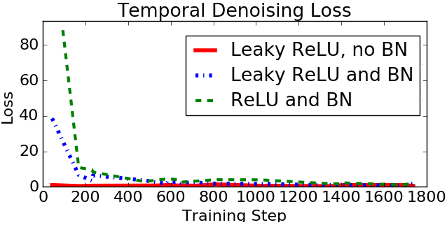
Figure 5: Evolution of the L2-Loss during the training of the Temporal-CNN. Batch Normalization (BN) does not help, adding a computation overhead without any improvement. With Leaky ReLU as activation function and with no BN, the loss starts immediately around 1 and decreases to $0.5$ after 60 epochs. Denoising without BN takes around $5\%$ less time. First 1800 steps visualized.

4.5 Exp 1: The Video Denoising CNN Architecture

The final proposed version of ViDeNN consists in two CNNs in a pipeline, performing first spatial and then temporal denoising. To get the final architecture, we trained ViDeNN with different structures and tested it on two famous benchmarking videos and on one we personally recorded with a Blackmagic Design URSA Mini 4.6K, capable to record raw videos. The videos have various levels of Additive White Gaussian Noise (AWGN). We will answer to three critical questions.

Q1: Is Temp3-CNN able to learn both temporal and spatial denoising?

We compare the Spatial-CNN with the Temp3-CNN, which in this case tries to perform spatial and temporal denoising at the same time.
Answer: No, Temp3 is not enough. Referring to Table 3, we notice how using Temp3-CNN alone leads to a worse result compared to the simpler Spatial-CNN.

Foreman Tennis Strijp-S * Res./Frames $288{\times}352$ / $300$ $240{\times}352$ / $150$ $656{\times}1164$/$787$ $\sigma$ $25$ $55$ $25$ $55$ $25$ Spatial-CNN 32.18 28.27 29.46 26.15 32.73 Temp3-CNN 31.56 27.45 29.32 25.63 31.13

Table 3: Comparison of Spatial-CNN and Temp3-CNN over videos with different levels of AWGN. The Temp3-CNN alone can not outperform the Spatial-CNN. Results expressed in terms of PSNR[dB]. *Self-recorded Raw video converted to RGB.

Q2: Ordering of spatial and temporal denoising? Knowing that using Temp3-CNN alone is not enough, we now have to compare different combination of spatial and temporal denoising.
Answer: looking at Table 4, we can confirm that using temporal denoising improves the result over spatial denoising, with the best performing combination as Spatial-CNN followed by Temp3-CNN.

Foreman Tennis Strijp-S Res./Frames $288{\times}352$ / $300$ $240{\times}352$ / $150$ $656{\times}1164$/$787$ $\sigma$ $25$ $55$ $25$ $55$ $25$ Spatial-CNN 32.18 28.27 29.46 26.15 32.73 Temp3-CNN & Spatial-CNN 32.09 28.37 29.21 25.98 32.28 Spatial-CNN & Temp3-CNN 33.12 29.56 30.36 27.18 34.07

Table 4: The combination of Spatial-CNN + Temp3-CNN is the best performing, showing consistent improvements of $\sim 1dB$ over the spatial-only denoising. Results expressed in terms of PSNR[dB].

Q3: How many frames to consider? We compare now the introduced Temp3-CNN with Temp5-CNN, which considers a time window of 5 frames.
Answer: Results in Table 5 shows that considering more frames could improve the result, but this is not guaranteed. Therefore, since using a bigger time window means more memory and time needed, we decided to use the three frames model for a better trade-off. For comparison, using the Temp5-CNN on the video Foreman took $6.5\%$ more time than using the Temp3-CNN, $21.17s$ vs $19.85s$ on GPU. The difference does not seem much here, but will enhance for realistic large videos.

Foreman Tennis Strijp-S Res./Frames $288{\times}352$ / $300$ $240{\times}352$ / $150$ $656{\times}1164$/$787$ $\sigma$ $25$ $55$ $25$ $55$ $25$ Spatial-CNN 32.18 28.27 29.46 26.15 32.73 Spatial-CNN & Temp3-CNN 33.12 29.56 30.36 27.18 34.07 Spatial-CNN & Temp5-CNN 33.03 29.87 30.72 27.70 33.97

Table 5: Comparison of architectures using 3 or 5 frames. Using a bigger time window, i.e. five frames, may slightly improve the final result or even worsen it. Hence, we decided to proceed using a 3-frames architecture. Results expressed in terms of PSNR[dB].

4.6 Exp 2: Sensitivity to Temporal Inconsistency

We investigate temporal consistency with a simple experiment where we remove an object from the first frame and the last frame where we denoise on the middle frame, see Figure 6. Specifically, (i) on the video Tennis from [41], add Gaussian noise with standard deviation $\sigma$=40; (ii) Manually remove the white ball on the first and last frame; (iii) Denoise the middle frame. In Figure 6 we show the modified input frames and ViDeNN output. In terms of PSNR value, we got the same value for both normal and experimental case: $27.28dB$. This is an illustration that the network does what we expected: it uses part of the secondary frames and combine them with the reference, but only where the pixel content is similar enough: the ball is not removed from frame 10.

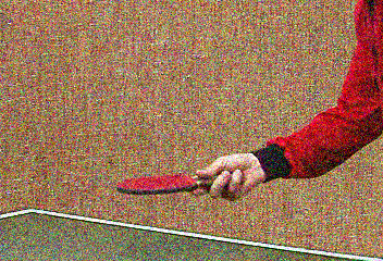
(a) Noisy Frame 9

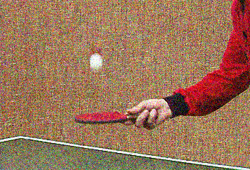
(b) Noisy Frame 10

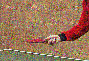
(c) Noisy Frame 11

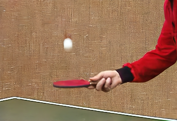
(d) Denoised Frame 10

Figure 6: ViDeNN achieves the same PSNR value of $27.28dB$ for frame 10 of the video Tennis with AWGN $\sigma$=40, even if we manually cancel the white ball from the secondary frames. The network understands which part has to take into consideration and which not, i.e. the ball area.

Visualization of temporal filters To understand what our model detects, we show in Figure 7 the output of two of the 128 filters in the first layer of Temp3-CNN. In Figure 7(a), we see in black the table-tennis ball of the current frame, whereas the ones in the previous and subsequent frame are in white. In Figure 7(b) instead, we see how this filter highlights flat areas with similar colors and shows mostly the ball of the current frame in white. Therefore, Temp3-CNN gives different importance to similar and different areas among the three frames. This is a simple indication on how the CNN handles motion and temporal inconsistencies.

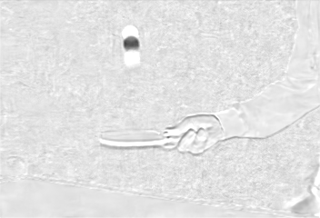
(a) Filter 90

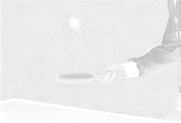
(b) Filter 59

Figure 7: Visualization of filters 59 and 90 output of Temp3-CNN first convolutional layer. We used frames number 9, 10 and 11 from the video Tennis as input. Filter 59 highlights the reference ball and other areas with similar colors, whereas filter 90 seems to highlight mostly contours and the ball at the reference position in frame 10.

Tennis Old Town Cross Park Run Stefan Res./Frames $240{\times}352$ / 150 $720{\times}1280$ / $500$ $720{\times}1280$ / $504$ $656{\times}1164$ / $300$ $\sigma$ $5$ $25$ $40$ $15$ $25$ $40$ $15$ $25$ $40$ $15$ $25$ $55$ ViDeNN 35.51 29.97 28.00 32.15 30.91 29.41 31.04 28.44 25.97 32.06 29.23 24.63 ViDeNN-G 37.81 30.36 28.44 32.39 31.29 29.97 31.25 28.72 26.36 32.37 29.59 25.06 VBM4D [10] 34.64 29.72 27.49 32.40 31.21 29.57 29.99 27.90 25.84 29.90 27.87 23.83 CBM3D [35] 27.04 26.37 25.62 28.19 27.95 27.35 24.75 24.46 23.71 26.19 25.89 24.18 DnCNN [14] 35.49 27.47 25.43 31.47 30.10 28.35 30.66 27.87 25.20 32.20 29.29 24.51

Table 6: Comparison of ViDeNN with a video denoising algorithm, VBM4D [10], and two image denoising algorithms, DnCNN [14] and CBM3D [35]. ViDeNN-G is the model trained specifically for blind Gaussian denoising. Test videos have different length, size and level of Additive White Gaussian Noise. ViDeNN performs better than blind denoising algorithms CBM3D, DnCNN and VBM4D, which has been used with the low complexity setup due to our memory limitations. Best results are highlighted in bold. Original videos are publicly available here [41]. Results expressed in terms of PSNR[dB].

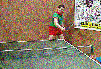
(a) Noisy frame
148

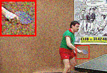
(b) Noisy frame
149

(c) Noisy frame
150

(d) CBM3D[6]
(25.60/0.9482)

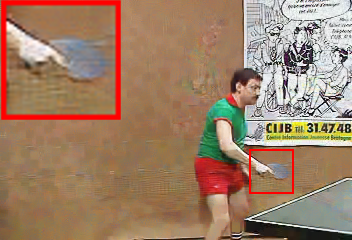
(e) VBM4D[10]
(24.51/0.9292)

(f) ViDeNN-G
(27.19/0.9605)

Figure 8: Blind video denoising comparison on Tennis [41] corrupted with AWGN $\sigma$=40 and values clipped between [0,255]. We show the result of two competitors, VBM4D and CBM3D, which scored respectively second and third (see Table 6) on this test video. ViDeNN performs well in challenging situations, even if the previous frame is completely different 8(a), thanks to the temporal inconsistency detection. VBM4D suffers from the change of view, creating artifacts. Results in brackets are referred to the single frame 149 (PSNR [dB]/SSIM).

Train Mountains Windmill Res./Frames $212{\times}1091$ / 4 $1080{\times}1920$ / 4 $1080{\times}1920$ / 3 Light 50/255 55/255 [55,75]/255 44.6 lux 118 lux 212 lux ViDeNN 34.05 36.96 40.84 32.96 35.42 36.69 VBM4D[10] 29.10 33.48 37.34 26.62 30.69 32.92 CBDNet[22] 30.89 34.56 39.91 29.56 34.31 36.22 CBM3D[35] 31.27 34.06 40.20 29.81 34.06 35.74 DnCNN[14] 24.33 29.87 32.39 21.73 25.55 27.87

Table 7: Comparison of state-of-art denoising algorithms over six low-light sequences recorded with a Bosch Autodome IP 5000 IR in raw mode, without any type of filtering activated. Every sequence is composed of 4 or 3 frames, with ground truths obtained averaging over 200 images. The Windmill sequences has been recorded with a different light source, where we were able to measure the light intensity. Highlighted in bold our ViDeNN results, which performs well. Results expressed in terms of PSNR[dB].

(a) Noisy frame 2
(22.54/0.4402)

(b) DnCNN [14]
(24.30/0.5323)

(c) VBM4D [10]
(29.08/0.7684)

(d) CBDNet [22]
(30.75/0.8710)

(e) CBM3D[35]
(31.11/0.8982)

(f) ViDeNN
(34.14/0.9158)

Figure 9: Detailed comparison of denoising algorithms on the low-light video Train with light intensity at 50/255. Our ViDeNN shows good performance in this light condition, preserving edges and correctly smoothing flat areas. Results referred to frame 2, expressed in terms of (PSNR [dB]/SSIM).

4.7 Exp 3: Evaluating Gaussian Video Denoising

Currently, most of the video and image denoising algorithms have been developed to tackle Additive White Gaussian Noise (AWGN). We will compare ViDeNN with the state-of-art algorithm for Gaussian video denoising VBM4D [10] and additionally with CBM3D [35] and DnCNN [14] for single frame denoising. We used the algorithms in their blind version: for VBM4D we activated the noise estimation, for CBM3D we set the sigma level to 50 and for DnCNN we use the blind model provided by the authors. We compare two versions of ViDeNN, where ViDeNN-G is the model trained specifically for AWGN denoising and ViDeNN is the final model tackling multiple noise models, including low-light conditions. The videos have been stored as uncompressed png frames, added with AWGN and saved again in loss-less png format. From the results in Table 6 we notice that VBM4D achieves superior results compared to its spatial counterpart CBM3D, which is probably due to the effectiveness of the noise estimator implemented in VBM4D. CBM3D suffers from the wrong noise std. deviation ($\sigma$) level for low noise intensities, whereas for high levels achieves comparable results. Overall, our implemented ViDeNN in its Gaussian specific version performs better than the general blind model, even though the difference is limited. ViDeNN-G scores the best results, as highlighted in bold in Table 6, confirming our blind video denoising network as a valid approach, which achieves state-of-art results.

4.8 Exp 4: Evaluating Low-Light Video Denoising

Along with the low-light dataset creation, we also recorded six sequences of three or four frames each:

• Two sequences of the same scene, with a moving toy train, in two different light intensities.

• A sequence of an artificial mountain landscape with increasing light intensity.

• Three sequences of the same scene, with a rotating toy windmill and a moving toy truck, in three different light conditions.

Those sequences are not part of the training set and have been recorded separately, with the same Bosch Autodome IP 5000 IR camera. In Table 7 we present the results of ViDeNN  highlighted in bold, in comparison with other state-of-art denoising algorithms on the low-light test set. We compare our method with VBM4D [10], CBM3D [35], DnCNN [14] and CBDNet [22]. ViDeNN outperforms the competitors, especially for the lowest light intensities. Surprisingly, the single frame denoiser CBM3D performs better than the video version VBM4D: the difference may be because CBM3D in its blind version uses $\sigma=50$, whereas VBM4D has a built-in noise level estimator, which may perform worse with a completely different noise model from the supposed Gaussian one.

5 Discussion

In this paper, we presented a novel CNN architecture for Blind Video Denoising called ViDeNN. We use spatial and temporal information in a feed-forward process, combining three consecutive frames to get a clean version of the middle frame. We perform temporal denoising in simple yet efficient manner, where our Temp3-CNN learns how to handle objects motion, brightness changes, and temporal inconsistencies. We do not address camera motion in videos, since the model was designed to reduce the bandwidth usage of static security cameras keeping the network as simple and efficient as possible. We define our model as Blind, since it can tackle different noise models at the same time, without any prior knowledge nor analysis of the input signal. We created a dataset containing multiple noise models, showing how the right mix of training data can improve image denoising on real world data, such as on the DND Benchmarking Dataset [31]. We achieve state-of-art results in blind Gaussian video denoising, comparing our outcome with the competitors available in the literature. We show how it is possible, with the proper hardware, to address low-light video denoising with the use of a CNN, which would ease the tuning of new sensors and camera models. Collecting the proper training data would be the most time consuming part. However, defining an automatic framework with predefined scenes and light conditions would simplify the process, allowing to further reduce the needed time and resources. Our technique for acquiring clean and noisy low-light image pairs has proven to be effective and simple, requiring no specific exposure tuning.

5.1 Limitations and Future Works

The largest real-world limitations of ViDeNN is the required computational power. Even with an high-end graphic card as the Nvidia Titan X, we were able to reach a maximum speed of only $\sim 3$fps on HD videos. However, most of the current cameras work with Full HD or even UHD (4K) resolutions with high frame rates. We did not try to implement ViDeNN on a mobile device supporting Tensorflow Lite, which converts the model to a lighter version more suitable for handled devices. This could be new development and challenging question to investigate on, since every week the available hardware in the market improves.

References

- [1] Ivana Despotović, Bart Goossens, and Wilfried Philips. Mri segmentation of the human brain: Challenges, methods, and applications. In Computational and Mathematical Methods in Medicine, volume 2015, pages 1–23. 05 2015.
- [2] Peter Goebel, Ahmed Nabil Belbachir, and Michael Truppe. A study on the influence of image dynamics and noise on the jpeg 2000 compression performance for medical images. In Computer Vision Approaches to Medical Image Analysis: Second International ECCV Workshop, volume 4241, pages 214–224. 05 2006.
- [3] Stefan Roth and Michael Black. Fields of experts: A framework for learning image priors. In Proceedings of the IEEE Computer Society Conference on Computer Vision and Pattern Recognition, volume 2, pages 860–867. 01 2005.
- [4] Jian Sun, Zongben Xu, and Heung-Yeung Shum. Image super-resolution using gradient profile prior. In 2008 IEEE Conference on Computer Vision and Pattern Recognition. 06 2008.
- [5] Huibin Li and Feng Liu. Image denoising via sparse and redundant representations over learned dictionaries in wavelet domain. In 2009 Fifth International Conference on Image and Graphics, pages 754–758. 09 2009.
- [6] Kostadin Dabov, Alessandro Foi, Vladimir Katkovnik, and Karen Egiazarian. Image denoising by sparse 3-d transform-domain collaborative filtering. In IEEE transactions on image processing, volume 16, pages 2080–95. 09 2007.
- [7] Julien Mairal, Francis Bach, J Ponce, Guillermo Sapiro, and Andrew Zisserman. Non-local sparse models for image restoration. In Proceedings of the IEEE International Conference on Computer Vision, pages 2272–2279. 09 2009.
- [8] Weisheng Dong, Lei Zhang, Guangming Shi, and Xin li. Nonlocally centralized sparse representation for image restoration. In IEEE transactions on image processing, volume 22. 12 2012.
- [9] Shuhang Gu, Lei Zhang, Wangmeng Zuo, and Xiangchu Feng. Weighted nuclear norm minimization with application to image denoising. In 2014 IEEE Conference on Computer Vision and Pattern Recognition, pages 2862–2869. 06 2014.
- [10] Matteo Maggioni, Giacomo Boracchi, Alessandro Foi, and Karen Egiazarian. Video denoising, deblocking, and enhancement through separable 4-d nonlocal spatiotemporal transforms. In IEEE transactions on image processing, volume 21, pages 3952–66. 05 2012.
- [11] Viren Jain and Sebastian Seung. Natural image denoising with convolutional networks. In D. Koller, D. Schuurmans, Y. Bengio, and L. Bottou, editors, Advances in Neural Information Processing Systems 21, pages 769–776. Curran Associates, Inc., 2009.
- [12] H.C. Burger, C.J. Schuler, and Stefan Harmeling. Image denoising: Can plain neural networks compete with bm3d? In 2012 IEEE Computer Society Conference on Computer Vision and Pattern Recognition, pages 2392–2399. 06 2012.
- [13] Bryan C. Russell, Antonio Torralba, Kevin Murphy, and William T. Freeman. Labelme: A database and web-based tool for image annotation. In International Journal of Computer Vision, volume 77. 05 2008.
- [14] Kai Zhang, Wangmeng Zuo, Yunjin Chen, Deyu Meng, and Lei Zhang. Beyond a gaussian denoiser: Residual learning of deep cnn for image denoising. In IEEE Transactions on Image Processing, volume 26, pages 3142–3155. 07 2017.
- [15] Sergey Ioffe and Christian Szegedy. Batch normalization: Accelerating deep network training by reducing internal covariate shift. In Proceedings of Machine Learning Research, volume 37, pages 448–456. 02 2015.
- [16] Kai Zhang, Wangmeng Zuo, and Lei Zhang. Ffdnet: Toward a fast and flexible solution for cnn based image denoising. In IEEE Transactions on Image Processing, volume 27, pages 4608 – 4622. 09 2018.
- [17] Dmitry Ulyanov, Andrea Vedaldi, and Victor Lempitsky. Deep image prior, 11 2017.
- [18] Stamatis Lefkimmiatis. Non-local color image denoising with convolutional neural networks. In 2017 IEEE Conference on Computer Vision and Pattern Recognition (CVPR), pages 5882 – 5891. 07 2017.
- [19] Dong Yang and Jian Sun. Bm3d-net: A convolutional neural network for transform-domain collaborative filtering. In IEEE Journals & Magazines, volume 25, pages 55 – 59. 01 2018.
- [20] Ying Tai, Jian Yang, Xiaoming Liu, and Chunyan Xu. Memnet: A persistent memory network for image restoration. pages 4539–4547, 10 2017.
- [21] Xiao-Jiao Mao, Chunhua Shen, and Yu-Bin Yang. Image denoising using very deep fully convolutional encoder-decoder networks with symmetric skip connections. In Advances in Neural Information Processing Systems 29, pages 2802–2810. 12 2016.
- [22] Shi Guo, Zifei Yan, Kai Zhang, Wangmeng Zuo, and Lei Zhang. Toward convolutional blind denoising of real photographs, 07 2018.
- [23] Jaakko Lehtinen, Jacob Munkberg, Jon Hasselgren, Samuli Laine, Tero Karras, Miika Aittala, and Timo Aila. Noise2noise: Learning image restoration without clean data. 2018.
- [24] Xiaokang Yang Xinyuan Chen, Li Song. Deep rnns for video denoising. In Proc. SPIE, volume 9971. 09 2016.
- [25] Simon Niklaus and Feng Liu. Context-aware synthesis for video frame interpolation. In The IEEE Conference on Computer Vision and Pattern Recognition (CVPR), 06 2018.
- [26] Simone Meyer, Abdelaziz Djelouah, Brian McWilliams, Alexander Sorkine-Hornung, Markus Gross, and Christopher Schroers. Phasenet for video frame interpolation. In The IEEE Conference on Computer Vision and Pattern Recognition (CVPR), 06 2018.
- [27] Jose Caballero, Christian Ledig, Andrew Aitken, Alejandro Acosta, Johannes Totz, Zehan Wang, and Wenzhe Shi. Real-time video super-resolution with spatio-temporal networks and motion compensation. In 2017 IEEE Conference on Computer Vision and Pattern Recognition (CVPR), pages 2848–2857, 07 2017.
- [28] Ren Yang, Mai Xu, Zulin Wang, and Tianyi Li. Multi-frame quality enhancement for compressed video. In 2018 IEEE Conference on Computer Vision and Pattern Recognition (CVPR), June 2018.
- [29] S. Su, M. Delbracio, J. Wang, G. Sapiro, W. Heidrich, and O. Wang. Deep video deblurring for hand-held cameras. In 2017 IEEE Conference on Computer Vision and Pattern Recognition (CVPR), pages 237–246, 07 2017.
- [30] Josue Anaya and Adrian Barbu. Renoir – a dataset for real low-light image noise reduction. In Journal of Visual Communication and Image Representation, volume 51, 09 2014.
- [31] Tobias Plotz and Stefan Roth. Benchmarking denoising algorithms with real photographs. In The IEEE Conference on Computer Vision and Pattern Recognition (CVPR), 07 2017.
- [32] Abdelrahman Abdelhamed, Stephen Lin, and Michael S. Brown. A high-quality denoising dataset for smartphone cameras. In The IEEE Conference on Computer Vision and Pattern Recognition (CVPR), 06 2018.
- [33] Chen Chen, Qifeng Chen, Jia Xu, and Vladlen Koltun. Learning to see in the dark. In The IEEE Conference on Computer Vision and Pattern Recognition (CVPR), 06 2018.
- [34] Bing Xu, Naiyan Wang, Tianqi Chen, and Mu Li. Empirical evaluation of rectified activations in convolutional network. 2015.
- [35] K. Dabov, A. Foi, V. Katkovnik, and K. Egiazarian. Color image denoising via sparse 3d collaborative filtering with grouping constraint in luminance-chrominance space. In 2007 IEEE International Conference on Image Processing, volume 1, pages I – 313–I – 316, 09 2007.
- [36] Kede Ma, Zhengfang Duanmu, Qingbo Wu, Zhou Wang, Hongwei Yong, Hongliang Li, and Lei Zhang. Waterloo Exploration Database: New challenges for image quality assessment models. volume 26, pages 1004–1016, 02 2017.
- [37] Diederik Kingma and Jimmy Ba. Adam: A method for stochastic optimization. In International Conference on Learning Representations, 12 2014.
- [38] Kai Zhang, Wangmeng Zuo, Yunjin Chen, Deyu Meng, and Lei Zhang. Dncnn matlab implementation on github, 2016.
- [39] CBSD68 benchmark dataset.
- [40] Darmstadt DND Benchmark Results.
- [41] Xiph.org Video Test Media [derf’s collection].