Prediction bounds for higher order total variation regularized least squares

Abstract

We establish adaptive results for trend filtering: least squares estimation with a penalty on the total variation of $(k-1)^{\rm th}$ order differences. Our approach is based on combining a general oracle inequality for the $\ell_{1}$-penalized least squares estimator with “interpolating vectors” to upper-bound the “effective sparsity”. This allows one to show that the $\ell_{1}$-penalty on the $k^{\text{th}}$ order differences leads to an estimator that can adapt to the number of jumps in the $(k-1)^{\text{th}}$ order differences of the underlying signal or an approximation thereof. We show the result for $k\in\{1,2,3,4\}$ and indicate how it could be derived for general $k\in\mathbb{N}$.

m[1]∥∥_0#1 m[1]∥∥_1#1 m[1]∥∥_2#1 rm[1]∥∥_n^2#1

and

1 Introduction

Total variation penalties have been introduced by Rudin et al. (1992) and Steidl et al. (2006). The present paper builds further on the theory as developed in Tibshirani (2014), Wang et al. (2016), and Guntuboyina et al. (2020). We show, for $k\in\{1,2,3,4\}$, a method for proving that the $k^{\text{th}}$ order total variation regularized least squares estimator adapts to the number of jumps in the $(k-1)^{\text{th}}$ order differences and indicate how this method could be generalized to any $k\in{\mathbb{N}}$. Inspired by Candès and Fernandez-Granda (2014), our main tool is a well-chosen vector interpolating the signs of the jumps.

The estimation method we will study is known as trend filtering. See Tibshirani (2020) for a comprehensive overview and connections. Trend filtering is a special case of the Lasso (Tibshirani (1996)): it is least squares estimation with an $\ell_{1}$-penalty on a subset of the coefficients. For trend filtering, the minimization problem can also be formulated as a so-called analysis problem (Elad et al. (2007)) with the analysis matrix $D$ being the $k^{\rm th}$ order differences operator (see Equation (2)). Our main result problem, given in Theorem 1.1, is based on an oracle inequality for the general analysis problem with arbitrary analysis matrix $D\in\mathbb{R}^{m\times n}$, as given in Theorem 2.2. The latter is a modification of results in Dalalyan et al. (2017): we generalize their projection arguments by allowing for adding “mock” variables to the active set. We furthermore use an improved version of their “compatibility constant” (see Remark 2.2) and - up to scaling - refer to its reciprocal as “effective sparsity”, see Definition 2.1. The effective sparsity for the Lasso problem is the number of active parameters (the sparsity) discounted by a factor due to correlations between variables. This discounting factor is called the compatibility constant (see Remark 2.2). In our situation the effective sparsity can be dealt with invoking what we call an “interpolating vector” (see Definition 2.3) which can be seen as a quantified noisy version of the so-called dual certificate used in basis pursuit. See Remark 2.3 for more details.

Consider an $n$-dimensional Gaussian vector of independent observations $Y\sim{\cal N}_{n}(f^{0},I)$ with unknown mean vector $f^{0}\in\mathbb{R}^{n}$, and with known variance ${\rm var}(Y_{i})=1$, $i=1,\ldots,n$ (see Remark 2.2 for the case of unknown variance). Let $D\in\mathbb{R}^{m\times n}$ be a given analysis matrix. The analysis estimator is

$$\hat{f}:=\arg\min_{f\in\mathbb{R}^{n}}\biggl{\{}\|Y-f\|_{n}^{2}+2\lambda\|Df\|_{1}\biggr{\}},$$ (1)

where we invoke the (abuse of) notation $\|v\|_{n}^{2}:=\sum_{i=1}^{n}v_{i}^{2}/n$, $v\in\mathbb{R}^{n}$. The general aim is to show that $\hat{f}$ is close to the mean $f^{0}:=\mathbb{E}Y$ of $Y$, or to some approximation $f\in\mathbb{R}^{n}$ thereof that has $\|D{f}\|_{0}$ “small”.

The trend filtering problem has as analysis matrix $D$ the $k^{\text{th}}$ order differences operator $\Delta(k)\in\mathbb{R}^{(n-k)\times n}$, which is defined as

$$\Delta(k)_{ij}:=\begin{dcases}(-1)^{l}\binom{k}{l},&j=i-l,\ l\in[0:k],\ i\in\mathcal{D},\\ 0,&\text{else},\end{dcases}$$ (2)

where $\mathcal{D}=[k+1:n]$ and $k\in[1:n-1]$ is fixed. We alternatively call $\Delta(k)$ the $k^{\rm th}$ order discrete derivative operator. Moreover, we apply the notation

$$[a:b]=\{j\in{\mathbb{N}}:a\leq j\leq b\},\ 0\leq a\leq b<\infty.$$

Theorem 2.2 below presents results for the general analysis problem and we apply it in Theorem 1.1 to the trend filtering problem. This application means that we need to introduce a “dictionary” as described in Subsection 2.2, to bound the lengths of the dictionary vectors, and finally calculate an interpolating vector to obtain a bound for the effective sparsity. We do the calculations for $k\in\{1,2,3,4\}$ and sketch the way to proceed for general $k\in{\mathbb{N}}$.

1.1 Related work

Total variation regularization and trend filtering have been studied from different angles in a variety of papers. The paper Mammen and van de Geer (1997) studies numerical adaptivity and rates of convergence. In Kim et al. (2009) it is shown that interior point methods work well for trend filtering. The paper Tibshirani (2014) clarifies connections with splines and also has minimax rates. In Wang et al. (2016) trend filtering on graphs is examined and it has theoretical error bounds in terms of the $\ell_{1}$-norm $\|Df\|_{1}$. The paper Sadhanala and Tibshirani (2017) contains theory for additive models with trend filtering. In Sadhanala et al. (2017) trend filtering in higher dimensions is studied and minimax rates are proved. The paper Chatterjee and Goswami (2019) proposes a recursive partitioning scheme for higher dimensional trend filtering. Our work is closely related to the paper Guntuboyina et al. (2020) which concerns the constrained problem as well as the penalized problem. Our results for the penalized problem with $k\in\{2,3,4\}$ improve those in Guntuboyina et al. (2020). As a special case we derive that under a “minimum length condition” saying that the distances between jumps of the $(k-1)^{\rm th}$ discrete derivative are all of the same order, and under an appropriate condition on the tuning parameter $\lambda$, the prediction error of the penalized least squares estimator is of order $(s_{0}+1)\log(n/(s_{0}+1))\log n/n$ where $s_{0}$ is the number of jumps of $\Delta(k-1)f^{0}$ (see Corollary 1.2). This is an improvement of the result in Guntuboyina et al. (2020) where the rate is shown to be $(s_{0}+1)^{2k}/n$ for $k\geq 2$. In fact, we show a more general result where $f^{0}$ may be replaced by a sparse approximation. For $k=1$ we show the result with a superfluous log-factor: it is known that in that case the rate of convergence for the prediction error is of order $(s_{0}+1)\log(n/(s_{0}+1))/n$, see Guntuboyina et al. (2020) and its references. Our extra log-factor is is due to the use of projection arguments instead of more refined empirical process theory. In van de Geer (2020) it is shown that the log-factor for $k=1$ can be removed when invoking entropy arguments instead of projections, while keeping the approach via interpolating vectors and effective sparsity.

The approach with interpolating vectors is in our view quite natural and lets itself be extended to other problems. We discuss this briefly in the concluding section, Section 4.

1.2 Organization of the paper

In the next subsection, Subsection 1.3, we present in Theorem 1.1 an adaptive result for trend filtering, where adaptivity means that the presented bound for the prediction error can be smaller when $f^{0}$ can be well approximated by a vector with fewer jumps in its $(k-1)^{\rm th}$ discrete derivative. Section 2 presents in Theorem 2.2 adaptive and non-adaptive bounds for the general analysis problem which will be our starting point for proving Theorem 1.1. We introduce effective sparsity and interpolating vectors in Definitions 2.1 and 2.3.

Section 3 applies the general result of Theorem 2.2 to the case $D=\Delta(k)$. We then need to introduce a projected dictionary for trend filtering, which is done in Subsection 3.1. With this we arrive at non-adaptive, almost minimax rates in Theorem 3.4. In Subsection 3.3 we construct interpolating vectors and bounds for the effective sparsity for the case $k\in\{1,2,3,4\}$ and also sketch how this can be done for general $k$. With these results in hand we finish in Subsection 3.4 the proof of the adaptive bounds for trend filtering with $k\in\{1,2,3,4\}$. Section 4 concludes the paper.

The appendix contains a proof of Theorem 2.2. Its arguments are to a large extent in Dalalyan et al. (2017) and Ortelli and van de Geer (2020), but there are modifications. The appendix also has the proofs for Subsection 3.1 and 3.3.

1.3 Main result for trend filtering

For $D=\Delta(k)$ and $\mathcal{D}=[k+1:n]$ we let $S=\{t_{1},\ldots,t_{s}\}\subseteq\mathcal{D},\ k+1\leq t_{1}<\ldots<t_{s}\leq n$ and let $t_{0}:=k$ and $t_{s+1}:=n+1$. We define $n_{i}=t_{i}-t_{i-1},\ i\in[1:s+1]$ and $n_{\rm max}:=\max_{1\leq i\leq s+1}n_{i}$. Moreover, for $f\in\mathbb{R}^{n}$ we write $(\Delta(k)f)_{-S}:=\{(\Delta(k)f)_{j}:\ j\in\mathcal{D}\backslash S\}$.

In Theorem 1.1 below, the set $S$ is fixed but arbitrary. The theorem presents an oracle inequality that allows for a trade-off between approximation error and estimation error by choosing $S$ and $f$ appropriately, depending on the unknown $f^{0}$. However, the tuning parameter will then depend on $s$. Remark 1.3 reverses this viewpoint.

Write for $u>0$,

$$\lambda_{0}(u):=\mathchoice{{\hbox{$\displaystyle\sqrt{2\log(2(n-k-s))+2u\over n\,}$}\lower 0.4pt\hbox{\vrule height=12.15277pt,depth=-9.72226pt}}}{{\hbox{$\textstyle\sqrt{2\log(2(n-k-s))+2u\over n\,}$}\lower 0.4pt\hbox{\vrule height=8.50694pt,depth=-6.80559pt}}}{{\hbox{$\scriptstyle\sqrt{2\log(2(n-k-s))+2u\over n\,}$}\lower 0.4pt\hbox{\vrule height=6.07639pt,depth=-4.86113pt}}}{{\hbox{$\scriptscriptstyle\sqrt{2\log(2(n-k-s))+2u\over n\,}$}\lower 0.4pt\hbox{\vrule height=6.07639pt,depth=-4.86113pt}}}.$$

Theorem 1.1 (Adaptive rates for $k=1,2,3,4$)

Let $k\in\{1,2,3,4\}$. There exists constants $c_{k}$ and $C_{k}$ depending only on $k$ such that the following holds.
Let $u>0$ be arbitrary and choose the tuning parameter $\lambda$ satisfying

$$\lambda\geq c_{k}n^{k-1}\biggl{(}{n_{\max}\over 2n}\biggr{)}^{2k-1\over 2}\lambda_{0}(u).$$

Let $f\in\mathbb{R}^{n}$ be arbitrary and define the signs

$$q_{t_{i}}:={\rm sign}(Df)_{t_{i}},\ i=[1:s].$$

Write $S^{\pm}:=\{i\in[2:s]:q_{t_{i}}q_{t_{i-1}}=-1\}\cup\{1,s+1\}$. Assume $n_{i}\geq k(k+2)$ for all $i\in S^{\pm}$. Finally, let $v>0$ be arbitrary. Then with probability at least $1-e^{-u}-e^{-v}$ we have

$$\lVert\hat{f}-f^{0}\rVert^{2}_{n} \leq \underbrace{\lVert f-f^{0}\rVert^{2}_{n}}_{\mbox{\it``approximation error"}}+4\lambda\lVert(\Delta(k)f)_{-S}\rVert_{1}$$

$$+ \underbrace{\left(\mathchoice{{\hbox{$\displaystyle\sqrt{\frac{k(s+1)}{n}\,}$}\lower 0.4pt\hbox{\vrule height=12.15277pt,depth=-9.72226pt}}}{{\hbox{$\textstyle\sqrt{\frac{k(s+1)}{n}\,}$}\lower 0.4pt\hbox{\vrule height=8.50694pt,depth=-6.80559pt}}}{{\hbox{$\scriptstyle\sqrt{\frac{k(s+1)}{n}\,}$}\lower 0.4pt\hbox{\vrule height=6.07639pt,depth=-4.86113pt}}}{{\hbox{$\scriptscriptstyle\sqrt{\frac{k(s+1)}{n}\,}$}\lower 0.4pt\hbox{\vrule height=6.07639pt,depth=-4.86113pt}}}+\mathchoice{{\hbox{$\displaystyle\sqrt{\frac{2v}{n}\,}$}\lower 0.4pt\hbox{\vrule height=8.59721pt,depth=-6.8778pt}}}{{\hbox{$\textstyle\sqrt{\frac{2v}{n}\,}$}\lower 0.4pt\hbox{\vrule height=6.01805pt,depth=-4.81447pt}}}{{\hbox{$\scriptstyle\sqrt{\frac{2v}{n}\,}$}\lower 0.4pt\hbox{\vrule height=4.2986pt,depth=-3.4389pt}}}{{\hbox{$\scriptscriptstyle\sqrt{\frac{2v}{n}\,}$}\lower 0.4pt\hbox{\vrule height=4.2986pt,depth=-3.4389pt}}}+\lambda\Gamma_{S}\right)^{2}}_{\mbox{\it``estimation error"}}$$

where

$$\Gamma_{S}^{2}=nC_{k}\left(\sum_{i\in S^{\pm}}{1+\log n_{i}\over n_{i}^{2k-1}}+\sum_{i\in S\backslash S^{\pm}}{1+\log n_{i}\over n_{\rm max}^{2k-1}}\right).$$ (3)

To prove this result, we will invoke Theorem 2.2. This requires providing a dictionary and bounding the effective sparsity given by Definition 2.1. In Subsection 3.4 we then put the pieces together.

Remark 1.1

The quantity $\Gamma_{S}^{2}$ in the above theorem is a bound for the effective sparsity.

Remark 1.2

One may take $c_{1}=c_{2}=2$. For $\min_{i\in S^{\pm}}n_{i}\rightarrow\infty$ asymptotic expressions for $c_{3}$ and $c_{4}$ can be taken to be $c_{3}\rightarrow 19/2$ and by numerical computation, $c_{4}\rightarrow 2\times 6^{7/2}/(18.62)\approx 56.83$. See Subsection 3.3.1.

Remark 1.3

The requirement for $\lambda$ depends on $S$. Therefore, given a fixed data-independent $\lambda$, the above theorem holds for the restricted selection of active sets $S$ having $n_{\max}$ upper bounded as

$$n_{\max}\leq\left(\frac{\mathchoice{{\hbox{$\displaystyle\sqrt{n\,}$}\lower 0.4pt\hbox{\vrule height=4.30554pt,depth=-3.44446pt}}}{{\hbox{$\textstyle\sqrt{n\,}$}\lower 0.4pt\hbox{\vrule height=4.30554pt,depth=-3.44446pt}}}{{\hbox{$\scriptstyle\sqrt{n\,}$}\lower 0.4pt\hbox{\vrule height=3.01389pt,depth=-2.41113pt}}}{{\hbox{$\scriptscriptstyle\sqrt{n\,}$}\lower 0.4pt\hbox{\vrule height=2.15277pt,depth=-1.72223pt}}}\lambda}{c_{k}\lambda_{0}(u)}\right)^{\frac{2}{2k-1}}.$$

Remark 1.4

In Section 3.3.1, we indicate how the bound of Theorem 1.1 could be established for general $k\in{\mathbb{N}}$.

We formulate a corollary for the case where the distances between jumps are all of the same order as the maximal distance $n_{\max}$. To facilitate the statement we give an asymptotic formulation. For sequences $\{a_{n}\}$ and $\{b_{n}\}$ in $(0,\infty)$ we use the notation $a_{n}={\mathcal{O}}(b_{n})$ if $\limsup_{n\rightarrow\infty}a_{n}/b_{n}<\infty$ and $a_{n}\asymp b_{n}$ if also $b_{n}/a_{n}={\mathcal{O}}(1)$. For a sequence of random variables $\{Z_{n}\}$ we write $Z_{n}={\mathcal{O}}_{\mathbb{P}}(1)$ if $\lim_{M\rightarrow\infty}\limsup_{n\rightarrow\infty}{\mathbb{P}}(|Z_{n}|>M)=0$.

Corollary 1.2

Fix $k\in\{1,2,3,4\}$. Choose $S$ such that

$$\min_{i\in[1:s+1]}n_{i}\asymp n_{\max}.$$

Then we can choose $\lambda$ of order

$$\lambda\asymp n^{k-1}\biggl{(}{1\over s+1}\biggr{)}^{2k-1\over 2}\mathchoice{{\hbox{$\displaystyle\sqrt{\log n\over n\,}$}\lower 0.4pt\hbox{\vrule height=11.04166pt,depth=-8.83337pt}}}{{\hbox{$\textstyle\sqrt{\log n\over n\,}$}\lower 0.4pt\hbox{\vrule height=7.72914pt,depth=-6.18335pt}}}{{\hbox{$\scriptstyle\sqrt{\log n\over n\,}$}\lower 0.4pt\hbox{\vrule height=5.52081pt,depth=-4.41667pt}}}{{\hbox{$\scriptscriptstyle\sqrt{\log n\over n\,}$}\lower 0.4pt\hbox{\vrule height=5.52081pt,depth=-4.41667pt}}}$$

and with this choice, for all $f\in\mathbb{R}^{n}$,

$$\lVert\hat{f}-f^{0}\rVert^{2}_{n} \leq \lVert f-f^{0}\rVert^{2}_{n}+4\lambda\lVert(\Delta(k)f)_{-S}\rVert_{1}$$

$$+ {\mathcal{O}}_{\mathbb{P}}\left(\frac{s+1}{n}\log(n/(s+1))\log n\right).$$

Remark 1.5

The requirement of Theorem 1.1 on the tuning parameter is more flexible than the one in Guntuboyina et al. (2020). For example, in the context of the above corollary, Guntuboyina et al. (2020) require $\lambda/n^{k-1}\asymp\mathchoice{{\hbox{$\displaystyle\sqrt{\log(n/(s+1))/n\,}$}\lower 0.4pt\hbox{\vrule height=7.5pt,depth=-6.00003pt}}}{{\hbox{$\textstyle\sqrt{\log(n/(s+1))/n\,}$}\lower 0.4pt\hbox{\vrule height=7.5pt,depth=-6.00003pt}}}{{\hbox{$\scriptstyle\sqrt{\log(n/(s+1))/n\,}$}\lower 0.4pt\hbox{\vrule height=5.25pt,depth=-4.20003pt}}}{{\hbox{$\scriptscriptstyle\sqrt{\log(n/(s+1))/n\,}$}\lower 0.4pt\hbox{\vrule height=3.75pt,depth=-3.00002pt}}}$. If we use this latter choice of the tuning parameter we find from Theorem 1.1

$$\lVert\hat{f}-f^{0}\rVert^{2}_{n} \leq \lVert f-f^{0}\rVert^{2}_{n}+4\lambda\lVert(\Delta(k)f)_{-S}\rVert_{1}$$

$$+ {\mathcal{O}}_{\mathbb{P}}\left(\frac{(s+1)^{2k}}{n}\log(n/(s+1))\log n\right).$$

Thus, up to log-terms Theorem 1.1 recovers the result of Guntuboyina et al. (2020), with $f=f^{0}$. We however obtain an improvement because we allow for a smaller tuning parameter. Moreover, we allow for a sparse approximation $f$ of $f^{0}$ and present a sharp oracle inequality. The paper Guntuboyina et al. (2020), also studies the constrained problem where they arrive at rates which are up to log-terms comparable to ours for the regularized problem when taking $f=f^{0}$.

Remark 1.6

Our method of proof is along the lines of Dalalyan et al. (2017). In Ortelli and van de Geer (2020) it is shown that one can also use this method for the square-root Lasso. This means that as a corollary of Ortelli and van de Geer (2020) our result also hold for “square-root” trend filtering, with a “universal” choice for the tuning parameter in the sense that it does not depend on the variance of the noise.

2 Adaptive bounds for the general analysis estimator

Recall the analysis problem

$$\hat{f}:=\arg\min_{f\in\mathbb{R}^{n}}\biggl{\{}\|Y-f\|_{n}^{2}+2\lambda\|Df\|_{1}\biggr{\}}$$ (4)

where $D\in\mathbb{R}^{m\times n}$ is a given analysis operator, $\lambda>0$ is a tuning parameter and $\lVert v\rVert^{2}_{n}:=\lVert v\rVert^{2}_{2}/n$, $v\in\mathbb{R}^{n}$.

To be able to state Theorem 2.2 - a modification of results in Dalalyan et al. (2017) (see Remark 2.2) - we introduce some notation in Subsection 2.1, and then describe the dictionary (Subsection 2.2) and the effective sparsity (Subsection 2.3). Theorem 2.2 can then be found in Subsection 2.4. To apply it one needs to upper-bound the effective sparsity. This is done in Lemma 2.4, which invokes interpolating vectors as defined in Definition 2.3 of Subsection 2.5. Theorem 2.2 and Lemma 2.4 combined serve as starting point for proving the result for trend filtering in Theorem 1.1.

2.1 Some notation

The rows of the analysis matrix $D\in\mathbb{R}^{m\times n}$ are indexed by a set $\mathcal{D}$ of size $\lvert\mathcal{D}\rvert=m$. We consider a set $S\subseteq\mathcal{D}$, which is arbitrary and can be chosen as the active set of an “oracle” that trades off “approximation error” and “estimation error” (see Theorem 2.2). The size of $S$ is denoted by $s:=|S|$. We define for a vector $b_{\mathcal{D}}\in\mathbb{R}^{m}$ with index set $\mathcal{D}$

$$b_{S}:=\{b_{j}\}_{j\in S},\ b_{-S}:=\{b_{j}\}_{j\in\mathcal{D}\backslash S}.$$

We let $\mathcal{N}_{-S}:=\{f\in\mathbb{R}^{n}:\ (Df)_{-S}=0\}=\{f\in\mathbb{R}^{n}:\ (Df)_{j}=0\ \forall\ j\in\mathcal{D}\backslash S\}$ and write $r_{S}:={\rm dim}({\cal N}_{-S})$. As benchmark for our result, consider the active set $S_{0}:=\{j:\ (Df^{0})_{j}\not=0\}$. If $S_{0}$ were known, the least squares estimator

$$\hat{f}_{\rm LSE}:=\arg\min_{f\in\mathcal{N}_{-S_{0}}}\|Y-f\|_{n}^{2}$$

would satisfy: for all $v>0$, with probability at least $1-\exp[-v]$

$$\|\hat{f}_{\rm LSE}-f^{0}\|_{n}\leq\mathchoice{{\hbox{$\displaystyle\sqrt{r_{S_{0}}\over n\,}$}\lower 0.4pt\hbox{\vrule height=9.40274pt,depth=-7.52223pt}}}{{\hbox{$\textstyle\sqrt{r_{S_{0}}\over n\,}$}\lower 0.4pt\hbox{\vrule height=6.9186pt,depth=-5.5349pt}}}{{\hbox{$\scriptstyle\sqrt{r_{S_{0}}\over n\,}$}\lower 0.4pt\hbox{\vrule height=5.62692pt,depth=-4.50156pt}}}{{\hbox{$\scriptscriptstyle\sqrt{r_{S_{0}}\over n\,}$}\lower 0.4pt\hbox{\vrule height=5.62692pt,depth=-4.50156pt}}}+\mathchoice{{\hbox{$\displaystyle\sqrt{2v\over n\,}$}\lower 0.4pt\hbox{\vrule height=8.59721pt,depth=-6.8778pt}}}{{\hbox{$\textstyle\sqrt{2v\over n\,}$}\lower 0.4pt\hbox{\vrule height=6.01805pt,depth=-4.81447pt}}}{{\hbox{$\scriptstyle\sqrt{2v\over n\,}$}\lower 0.4pt\hbox{\vrule height=4.2986pt,depth=-3.4389pt}}}{{\hbox{$\scriptscriptstyle\sqrt{2v\over n\,}$}\lower 0.4pt\hbox{\vrule height=4.2986pt,depth=-3.4389pt}}}.$$

This follows from a concentration bound for chi-squared random variables, see Lemma 1 in Laurent and Massart (2000). An aim is to show that the estimator $\hat{f}$ converges with the same rate $\textstyle\sqrt{r_{S_{0}}/n\,}$ , modulo log-factors. In fact we aim at showing this type of result with $f^{0}$ potentially replaced by a sparse approximation. We hope to be able to choose the active set $S$ of a sparse approximation such that $r_{S}$ is small. On the other hand, as we will see, the distance of the “non-active” variables to the linear space ${\cal N}_{-S}$ will play an important role: the smaller this distance, the less noise is left to be overruled by the penalty. Therefore, we allow for the possibility to extend $\mathcal{N}_{-S}$ to a larger linear space $\bar{\cal N}_{-S}\supseteq\mathcal{N}_{-S}$. This can be done for instance by adding some “mock” active variables to the active set. We let $\bar{r}_{S}={\rm dim}(\bar{\mathcal{N}}_{-S})$. Thus, $\bar{r}_{S}\geq r_{S}$ but in our application to trend filtering we will choose them of the same order.

2.2 The dictionary

Given the linear space $\bar{\mathcal{N}}_{-S}\supseteq\mathcal{N}_{-S}$ we can decompose a vector $f\in\mathbb{R}^{n}$ into its projection $f_{{\bar{\mathcal{N}}}_{-S}}$ onto $\bar{\mathcal{N}}_{-S}$ and its projection onto the ortho-complement $\bar{\mathcal{N}}_{-S}^{\perp}$, which we call its anti-projection:

$$f=f_{{\bar{\mathcal{N}}}_{-S}}+f_{{\bar{\mathcal{N}}}_{-S}^{\perp}}.$$

The anti-projection is the part we want to overrule by the penalty. For this purpose, we define a dictionary $\Psi^{-S}:=\{\psi_{j}^{-S}\}_{j\in\mathcal{D}\backslash S}\in\mathbb{R}^{n\times(m-s)}$ such that for all $f\in\mathbb{R}^{n}$ and for $b_{-S}=(Df)_{-S}$

$$f_{{\bar{\mathcal{N}}}_{-S}^{\perp}}=\Psi^{-S}b_{-S}.$$

In general there can be several choices for $\Psi^{-S}$. In the application to trend filtering that we consider in this paper, $\Psi^{-S}$ will be uniquely defined (when $\bar{\mathcal{N}}_{S}=\mathcal{N}_{-S}$ it holds that $\Psi^{-S}=D_{-S}^{\prime}(D_{-S}D_{-S}^{\prime})^{-1}$ with $D_{-S}$ being the matrix $D$ with the rows indexed by $S$ removed).

2.3 Effective sparsity

The effective sparsity will be invoked to establish adaptive bounds.

Fix some $u>0$. Its value will occur in the confidence level of the inequalities in Theorem 2.2. We define

$$\lambda_{0}(u):=\mathchoice{{\hbox{$\displaystyle\sqrt{2\log(2(m-s))+2u)\over n\,}$}\lower 0.4pt\hbox{\vrule height=12.15277pt,depth=-9.72226pt}}}{{\hbox{$\textstyle\sqrt{2\log(2(m-s))+2u)\over n\,}$}\lower 0.4pt\hbox{\vrule height=8.50694pt,depth=-6.80559pt}}}{{\hbox{$\scriptstyle\sqrt{2\log(2(m-s))+2u)\over n\,}$}\lower 0.4pt\hbox{\vrule height=6.07639pt,depth=-4.86113pt}}}{{\hbox{$\scriptscriptstyle\sqrt{2\log(2(m-s))+2u)\over n\,}$}\lower 0.4pt\hbox{\vrule height=6.07639pt,depth=-4.86113pt}}}.$$ (5)

In what follows, we assume that the tuning parameter $\lambda$ satisfies

$$\lambda\geq\max_{j\in\mathcal{D}\backslash S}\|\psi_{j}^{-S}\|_{n}\lambda_{0}(u).$$ (6)

For a vector $w_{-S}$ with $0\leq w_{j}\leq 1$ for all $j\in\mathcal{D}\backslash S$ we write

$$(1-w_{-S})(Df)_{-S}:=\{(1-w_{j})(Df)_{j}\}_{j\in\mathcal{D}\backslash S}.$$

Definition 2.1 (Effective sparsity)

Let $q_{S}\in\{-1,+1\}^{s}$ be a sign vector. The noiseless effective sparsity is

$$\Gamma^{2}(q_{S}):=\left(\max\biggl{\{}q_{S}^{\prime}(Df)_{S}-\|(Df)_{-S}\|_{1}:\ \|f\|_{n}=1\biggr{\}}\right)^{2}.$$

The noisy effective sparsity is defined as

$$\Gamma^{2}(q_{S},w_{-S}):=\left(\max\biggl{\{}\ q_{S}^{\prime}(Df)_{S}-\|(1-w_{-S}(Df)_{-S}\|_{1}:\ \|f\|_{n}=1\biggr{\}}\right)^{2},$$

where

$$w_{j}=\|\psi_{j}^{-S}\|_{n}\lambda_{0}(u)/\lambda,\ j\in\mathcal{D}\backslash S,$$

with $\lambda$ satisfying (6).

Remark 2.1

On the slightly negative side, when applying Theorem 2.2 one may need to choose $\lambda$ strictly larger than (but of the same order as) required in (6) in order to have a “well-behaved” effective sparsity. On the positive side, depending on the situation, one may improve upon $\lambda_{0}(u)$ in (5) using bounds for weighted empirical processes.

2.4 Main result for the general analysis problem

Recall that the set $S$ is arbitrary. In the following theorem, the set $S$ and also its vector $f\in\mathbb{R}^{n}$ can be chosen to optimize the bounds by trading off approximation error and estimation error. The theorem provides adaptive bounds (oracle inequalities) since the trade-off depends on the unknown signal $f^{0}$.

Theorem 2.2

Let $u>0$, $v>0$ and let the tuning parameter $\lambda$ satisfy (6). Then $\forall f\in\mathbb{R}^{n}$ the following bounds hold:

• a non-adaptive bound: with probability at least $1-e^{-u}-e^{-v}$,

  $$\lVert\hat{f}-f^{0}\rVert^{2}_{n} \leq \lVert f-f^{0}\rVert^{2}_{n}+4\lambda\lVert Df\rVert_{1}$$

  $$+ \left(\mathchoice{{\hbox{$\displaystyle\sqrt{\frac{\bar{r}_{S}}{n}\,}$}\lower 0.4pt\hbox{\vrule height=9.74387pt,depth=-7.79514pt}}}{{\hbox{$\textstyle\sqrt{\frac{\bar{r}_{S}}{n}\,}$}\lower 0.4pt\hbox{\vrule height=8.55138pt,depth=-6.84114pt}}}{{\hbox{$\scriptstyle\sqrt{\frac{\bar{r}_{S}}{n}\,}$}\lower 0.4pt\hbox{\vrule height=8.12082pt,depth=-6.49669pt}}}{{\hbox{$\scriptscriptstyle\sqrt{\frac{\bar{r}_{S}}{n}\,}$}\lower 0.4pt\hbox{\vrule height=8.12082pt,depth=-6.49669pt}}}+\mathchoice{{\hbox{$\displaystyle\sqrt{\frac{2v}{n}\,}$}\lower 0.4pt\hbox{\vrule height=8.59721pt,depth=-6.8778pt}}}{{\hbox{$\textstyle\sqrt{\frac{2v}{n}\,}$}\lower 0.4pt\hbox{\vrule height=6.01805pt,depth=-4.81447pt}}}{{\hbox{$\scriptstyle\sqrt{\frac{2v}{n}\,}$}\lower 0.4pt\hbox{\vrule height=4.2986pt,depth=-3.4389pt}}}{{\hbox{$\scriptscriptstyle\sqrt{\frac{2v}{n}\,}$}\lower 0.4pt\hbox{\vrule height=4.2986pt,depth=-3.4389pt}}}\right)^{2}.$$

• and an adaptive bound: with probability at least $1-e^{-u}-e^{-v}$,

  $$\lVert\hat{f}-f^{0}\rVert^{2}_{n} \leq \lVert f-f^{0}\rVert^{2}_{n}+4\lambda\lVert(Df)_{-S}\rVert_{1}$$

  $$+ \left(\mathchoice{{\hbox{$\displaystyle\sqrt{\frac{\bar{r}_{S}}{n}\,}$}\lower 0.4pt\hbox{\vrule height=9.74387pt,depth=-7.79514pt}}}{{\hbox{$\textstyle\sqrt{\frac{\bar{r}_{S}}{n}\,}$}\lower 0.4pt\hbox{\vrule height=8.55138pt,depth=-6.84114pt}}}{{\hbox{$\scriptstyle\sqrt{\frac{\bar{r}_{S}}{n}\,}$}\lower 0.4pt\hbox{\vrule height=8.12082pt,depth=-6.49669pt}}}{{\hbox{$\scriptscriptstyle\sqrt{\frac{\bar{r}_{S}}{n}\,}$}\lower 0.4pt\hbox{\vrule height=8.12082pt,depth=-6.49669pt}}}+\mathchoice{{\hbox{$\displaystyle\sqrt{\frac{2v}{n}\,}$}\lower 0.4pt\hbox{\vrule height=8.59721pt,depth=-6.8778pt}}}{{\hbox{$\textstyle\sqrt{\frac{2v}{n}\,}$}\lower 0.4pt\hbox{\vrule height=6.01805pt,depth=-4.81447pt}}}{{\hbox{$\scriptstyle\sqrt{\frac{2v}{n}\,}$}\lower 0.4pt\hbox{\vrule height=4.2986pt,depth=-3.4389pt}}}{{\hbox{$\scriptscriptstyle\sqrt{\frac{2v}{n}\,}$}\lower 0.4pt\hbox{\vrule height=4.2986pt,depth=-3.4389pt}}}+\lambda\Gamma(q_{S},w_{-S})\right)^{2},$$

  where $q_{S}=\text{sign}(Df)_{S}$.

Proof of Theorem 2.2.

See Appendix A. ∎

Remark 2.2

Theorem 2.2 is a modification of the findings by Dalalyan et al. (2017) who study the Lasso problem. Theorem 2.2 is in terms of the analysis problem, as in Ortelli and van de Geer (2020). We furthermore allow for augmentation of $\mathcal{N}_{-S}$. Moreover, Dalalyan et al. (2017) and Ortelli and van de Geer (2020) replace $\Gamma(q_{S},w_{-S})$ by the larger quantity $\max\{\ \|(Df)_{S}\|_{1}-\|(1-w_{-S})(Df)_{-S}\|_{1}:\|f\|_{n}=1\}=:\mathchoice{{\hbox{$\displaystyle\sqrt{r_{S}\,}$}\lower 0.4pt\hbox{\vrule height=4.30554pt,depth=-3.44446pt}}}{{\hbox{$\textstyle\sqrt{r_{S}\,}$}\lower 0.4pt\hbox{\vrule height=4.30554pt,depth=-3.44446pt}}}{{\hbox{$\scriptstyle\sqrt{r_{S}\,}$}\lower 0.4pt\hbox{\vrule height=3.01389pt,depth=-2.41113pt}}}{{\hbox{$\scriptscriptstyle\sqrt{r_{S}\,}$}\lower 0.4pt\hbox{\vrule height=2.15277pt,depth=-1.72223pt}}}/\kappa(S,w_{-S})$ where $\kappa^{2}(S,w_{-S})$ is called the “compatibility constant”. The paper Ortelli and van de Geer (2020) derives oracle results for the square-root analysis problem, which is the analysis version of the square-root Lasso introduced by Belloni et al. (2011). Joining these findings allows to derive a square-root version of Theorem 2.2 which can be applied to the case of unknown noise variance (see also Remark 1.6).

2.5 Interpolating vectors

To upper-bound the effective sparsity one may invoke interpolating vectors.

Definition 2.3 (Interpolating vector)

Let $q_{S}\in\{-1,+1\}^{s}$ be a sign vector. We call the completed vector $q\in\mathbb{R}^{m}$ with index set $\mathcal{D}$ an interpolating vector (that interpolates the given signs at $S$).

Lemma 2.4

Let $q_{S}\in\{-1,+1\}^{s}$ be a sign vector. The noiseless effective sparsity satisfies

$$\Gamma^{2}(q_{S})\leq\inf\{n\|D^{\prime}q\|_{2}^{2}:\ q\ \mbox{interpolating},\ |q_{j}|\leq 1\ \forall\ j\in\mathcal{D}\backslash S\}.$$

The noisy effective sparsity $\Gamma(q_{S},w_{-S})$ satisfies

$$\Gamma^{2}(q_{S},w_{-S})\leq\inf\{n\|D^{\prime}q\|_{2}^{2}:\ q\ \mbox{interpolating},\ |q_{j}|\leq 1-w_{j}\ \forall\ j\in\mathcal{D}\backslash S\},$$

where

$$w_{j}=\|\psi_{j}^{-S}\|_{n}\lambda_{0}(u)/\lambda,\ j\in\mathcal{D}\backslash S,$$

with $\lambda$ satisfying (6).

Proof of Lemma 2.4.

We only prove the statement of the lemma for the noisy case as the argument is the same for the noiseless case. For any vector $q_{-S}$ with $|q_{j}|\leq 1-w_{j}$ for all $j\in\mathcal{D}\backslash S$, it is true that for all $f$,

$$\|(1-w_{-S})(Df)_{-S}\|_{1}\geq q_{-S}(Df)_{-S}.$$

Therefore, for all $f$,

$$q_{S}^{\prime}(Df)_{S}-\|(1-w_{-S})(Df)_{-S}\|_{1}\leq q^{\prime}Df\leq\mathchoice{{\hbox{$\displaystyle\sqrt{n\,}$}\lower 0.4pt\hbox{\vrule height=4.30554pt,depth=-3.44446pt}}}{{\hbox{$\textstyle\sqrt{n\,}$}\lower 0.4pt\hbox{\vrule height=4.30554pt,depth=-3.44446pt}}}{{\hbox{$\scriptstyle\sqrt{n\,}$}\lower 0.4pt\hbox{\vrule height=3.01389pt,depth=-2.41113pt}}}{{\hbox{$\scriptscriptstyle\sqrt{n\,}$}\lower 0.4pt\hbox{\vrule height=2.15277pt,depth=-1.72223pt}}}\lVert D^{\prime}q\rVert_{2}\lVert f\rVert_{n}.$$

∎

Remark 2.3

To bound the effective sparsity invoking interpolating vectors, as the above lemma does, we were inspired by the dual certificates as applied in Candès and Fernandez-Granda (2014). These have also been used in other works. The paper Candès and Fernandez-Granda (2014) considers the superresolution problem and develops an interpolating function to establish exact recovery in the noiseless problem. The requirement on this interpolating function is that it is in the range of the transpose of the design matrix. Dual certificates can be found in earlier work as well, see for example Candès and Plan (2011). The latter applies a “near” dual certificate to deal with noisy measurements. However, their “nearness” appears to be restricted to a special setting. In Tang et al. (2014) the approach is related to ours but very much tied down to the noisy superresolution problem. We are not aware of any work where an explicit connection is made between dual certificates and compatibility constants, the latter being related to the reciprocal of effective sparsity: see Remark 2.2. The relation between dual certificates and interpolating vectors on the one hand and compatibility on the other hand, appears to have been hidden in the literature. Moreover, the notion of compatibility has developed itself over the years. In for example Boyer et al. (2017) it is shown that compatibility conditions do not hold for superresolution, but they show it for an older version of compatibility, not for the newer version based on $\kappa^{2}(S,w_{-S})$.

3 Application of Theorem 2.2 when $D=\Delta(k)$

In order to apply Theorem 2.2 with $D=\Delta(k)$ we need to establish a bound for the length of the columns of an appropriate dictionary $\Psi^{-S}$. This is done in Subsection 3.1. Then we can apply the first part of Theorem 2.2 and this will, as we will see in Subsection 3.2, result in the minimax rate up to log-terms. Next, for the application of the second part of Theorem 2.2 to obtain adaptive results, we upper-bound the effective sparsity using an appropriate interpolating vector. This is done in Subsection 3.3. We then have all the material to establish Theorem 1.1 as is summarized in Subsection 3.4.

3.1 The dictionary when $D=\Delta(k)$

We start with some remarks, whose purpose is mainly to introduce some further notation. Note that by definition, ${\cal N}_{\mathcal{D}}:=\{f\in\mathbb{R}^{n}:\ (Df)_{j}=0\ \forall\ j\in\mathcal{D}\}$. For vectors $f_{{\cal N}_{\mathcal{D}}}^{\perp}$ a dictionary is denoted by $\Psi^{\mathcal{D}}$. If $D$ has full row rank (which will be the case for $D=\Delta(k)$, see Wang et al. (2014)) it holds that $\Psi^{\cal D}=D^{\prime}(DD^{\prime})^{-1}$. This is the Moore Penrose pseudo inverse $D^{+}$ of $D$. Let now $\Psi=\{\psi_{j}\}_{j=1}^{n}\in\mathbb{R}^{n\times n}$ be a “complete” dictionary, which means that we can write each $f\in\mathbb{R}^{n}$ as $f=\Psi b$, where $b_{\cal D}=Df$. Then obviously $\Psi^{\mathcal{D}}=\{(\psi_{j})_{{\cal N}_{\mathcal{D}}^{\perp}}\}_{j\in{\cal D}}$ is formed by the projections of the dictionary vectors $\psi_{j}$ with index in ${\cal D}$ on the ortho-complement of the space spanned by $\{\psi_{j^{\prime}}\}_{j^{\prime}\notin\mathcal{D}}$. Moreover the dictionary $\Psi^{-S}=\{\psi_{j}^{-S}\}_{j\in\mathcal{D}\backslash S}$ for vectors $f_{{\cal N}_{-S}}^{\perp}$ has $\psi_{j}^{-S}=(\psi_{j})_{{\cal N}_{-S}^{\perp}}=(\psi_{j}^{\mathcal{D}})_{{\cal N}_{-S}^{\perp}}$.

As said, we may want to augment the space ${\mathcal{N}}_{-S}$ to a larger linear space $\bar{\mathcal{N}}_{-S}$ so that the anti-projections will have smaller length. This is done by taking the direct product of ${\cal N}_{-S}$ with a space spanned by additional linearly independent vectors $\{\phi_{j}\}$ with $\phi_{j}\notin{\cal N}_{-S}$ for all $j$. We call these additional vectors “mock” variables. One may pick them in the set $\{\psi_{j}\}_{j\in\mathcal{D}\backslash S}$ (or $\{\psi_{j}^{\mathcal{D}}\}_{j\in\mathcal{D}\backslash S}$) in which case we call them “mock” active variables.

We now first present upper bounds for $\{\|\psi_{j}\|_{2}^{2}\}_{j\in{\cal D}\backslash S}$ for the case $D=\Delta(k)$ for general $k$. We then give exact expressions for $k\in\{1,2,3\}$ to illustrate that the bounds are sharp.

3.1.1 The dictionary for general $k$: upper bounds

We take $\bar{\mathcal{N}}_{-S}$ as the direct product of $\mathcal{N}_{-S}$ and the space spanned by $\{\psi_{t_{i}+1},\ldots\psi_{t_{i}+k-1}\}_{i=1}^{s}$ (assuming $t_{s}+k-1\leq n$). In this way we disconnect the system into $s+1$ components each having the same structure. The matrix $D$ with the rows indexed by $S\cup\{t_{i}+1,\ldots,t_{i}+k-1\}_{i=1}^{s}$ removed is a block matrix. To avoid digressions more details are given below only for $k\in\{1,2,3\}$ but it is clear that such a disconnection works for general $k$. The space $\bar{\mathcal{N}}_{-S}$ has dimension $\bar{r}_{S}=r_{S}+s(k-1)=k(s+1)$. One may apply a reformulation for the sub-intervals $\{[t_{i-1}+1:t_{i}-1]\}_{i=1}^{s+1}$, to arrive at upper bounds for the lengths of the columns of $\Psi^{-S}$ from upper bounds for the lengths of the columns of $\Delta(k)^{+}$.

Lemma 3.1 (An upper bound for the length of the columns of $\Delta(k)^{+}$.)

We have that for $j\in[k+1:n-1]$

$$\lVert\psi_{j}^{\cal D}\rVert_{2}^{2}\leq\min\biggl{(}(j-k)^{2k-1},(n+1-j)^{2k-1}\biggr{)}.$$

Proof of Lemma 3.1.

See Appendix B. ∎

It follows that

$$\|\psi_{t_{i-1}+j}^{-S}\|_{2}^{2}\leq\min\biggl{(}j^{2k-1},(n_{i}-j)^{2k-1}\biggr{)},\ j\in[1:n_{i}-1],\ i=[1:s+1].$$ (7)

Recall our abuse of notation $\|\cdot\|_{n}^{2}=\|\cdot\|_{2}^{2}/n$. We get

$$\max_{j\in[1:n_{i}-1]}\|\psi_{t_{i-1}+j}^{-S}\|_{n}^{2}\leq{(n_{i}/2)^{2k-1}\over n},\ i=[1:s+1].$$

We conclude that the requirement (6) on the tuning parameter is met when

$$\lambda\geq n^{k-1}\biggl{(}{n_{\rm max}\over 2n}\biggr{)}^{2k-1\over 2}\mathchoice{{\hbox{$\displaystyle\sqrt{2\log(2(n-s-k))+2u\over n\,}$}\lower 0.4pt\hbox{\vrule height=12.15277pt,depth=-9.72226pt}}}{{\hbox{$\textstyle\sqrt{2\log(2(n-s-k))+2u\over n\,}$}\lower 0.4pt\hbox{\vrule height=8.50694pt,depth=-6.80559pt}}}{{\hbox{$\scriptstyle\sqrt{2\log(2(n-s-k))+2u\over n\,}$}\lower 0.4pt\hbox{\vrule height=6.07639pt,depth=-4.86113pt}}}{{\hbox{$\scriptscriptstyle\sqrt{2\log(2(n-s-k))+2u\over n\,}$}\lower 0.4pt\hbox{\vrule height=6.07639pt,depth=-4.86113pt}}}.$$ (8)

3.1.2 The dictionary when $k=1$: exact expressions

The case $k=1$ has been well studied, see Guntuboyina et al. (2020) and its references. We include it here and later in Subsection 3.3.2 to highlight the additional argument needed when $k>1$. We choose $\bar{\mathcal{N}}_{-S}=\mathcal{N}_{-S}$: no augmentation of this null space. In the present case $D$ is the incidence matrix of a path graph:

$$D=\Delta(1):=\begin{pmatrix}1&-1&0&\cdots&0&0\cr 0&1&-1&\cdots&0&0\cr 0&0&1&\cdots&0&0\cr\vdots&\vdots&\vdots&\ddots&\vdots&\vdots\cr 0&0&0&\cdots&1&-1\cr\end{pmatrix}.$$

Thus by removing the rows in $S$ we see that we turn the matrix into a block matrix consisting of $s+1$ row-wise orthogonal submatrices that have, apart from columns consisting of only zero’s, the same structure as the original matrix $D$. It means that the dictionary $\Psi^{-S}$ is of the same form as the dictionary $\Psi^{\cal D}$ for the vectors $f$ in deviation from their mean. It is easy to see that this dictionary is

$$\psi_{i,j}^{\mathcal{D}}={j-1\over n}{\rm l}\{j\leq i\}-{n-j+1\over n}{\rm l}\{j>i\},i\in[1:n],\ j\in[2:n].$$

The matrix $\Psi^{\cal D}\in\mathbb{R}^{n\times(n-1)}$ has squared column lengths

$$\|\psi_{j}^{\mathcal{D}}\|_{2}^{2}={(j-1)(n-j+1)\over n},\ j\in[2:n].$$

It follows that for $i=1,\ldots,s+1$ and $j\in[1:n_{i}-1]$,

$$\|\psi_{t_{i-1}+j}^{-S}\|_{2}^{2}={j(n_{i}-j)\over n_{i}}.$$

3.1.3 The dictionary when $k=2$: exact expressions

When the analysis operator $D$ is equal to $\Delta(2)$ its expression is

$$D=\Delta(2)=\begin{pmatrix}1&-2&1&0&\cdots&0&0&0\cr 0&1&-2&1&\cdots&0&0&0\cr 0&0&1&-2&\cdots&0&0&0\cr\vdots&\vdots&\vdots&\vdots&\ddots&\vdots&\vdots\cr 0&0&0&0&\cdots&1&-2&1\cr\end{pmatrix}.$$

Therefore by removing only the rows in $S$ the matrix we end up with is no longer consisting of row-wise orthogonal sub-matrices. However, if we remove two rows at the time, those in $S$ together with their immediate followers $\{t_{i}+1\}_{i=1}^{s}$ (for $t_{s}+1\leq n$ as otherwise at that point there is nothing to remove), we again obtain $s+1$ sub-matrices that are, apart from their columns consisting of only zero’s, of the same form as $D$. The dictionary $\Psi^{-S}$ for functions $f_{\mathcal{N}_{-S}^{\perp}}$ has thus the same form as the dictionary $\Psi^{\mathcal{D}}$ for the functions $f_{\mathcal{N}_{\mathcal{D}}^{\perp}}$, which are functions $f$ in deviation from their projections on their linear part. Therefore it is useful to augment $\mathcal{N}_{-S}$ by taking its direct product with the linear space spanned by the mock active variables $\{\psi_{t_{i}+1}\}_{i=1}^{s}$ to form $\bar{\mathcal{N}}_{-S}$. Note that $\bar{r}_{S}=r_{S}+s=2(s+1)$. Recall that $\Psi^{\mathcal{D}}$ is the Moore Penrose pseudo inverse $D^{+}$, in this case $\Delta(2)^{+}$. We present the exact column lengths of $\Delta(2)^{+}$ here: they show that the upper bounds of Lemma 3.1 are, up to constants, sharp.

Lemma 3.2 (Length of the columns of $\Delta(2)^{+}$.)

The length of the columns $\{\psi^{\mathcal{D}}_{j}\}_{j\in[n]\setminus[2]}$ of the Moore Penrose inverse $\Psi^{\mathcal{D}}=\Delta(2)^{+}$ is (for $j\in[3:n]$)

$$\lVert\psi^{\mathcal{D}}_{j}\rVert^{2}_{2}=\frac{(n-j+1)(n-j+2)(j-2)(j-1)(2j(n-j+3)-3(n+1))}{6n(n+1)(n-1)}.$$

Proof of Lemma 3.2.

See Appendix B. ∎

3.1.4 The dictionary when $k=3$: exact expressions

When $k=3$ we form $\bar{\mathcal{N}}_{-S}$ by taking the direct product of the linear space $\mathcal{N}_{-S}$ and the space spanned by $\{\psi_{t_{i}+1},\psi_{t_{i}+2}\}_{i=1}^{s}$ (assuming $t_{s}+2\leq n$). This space has dimension $\bar{r}_{S}=r_{S}+2s=3(s+1)$. The dictionary $\Psi^{-S}$ has blocks of the same form as the Moore Penrose pseudo inverse $\psi^{\mathcal{D}}=\Delta(3)^{+}$. We compute the exact length of the columns of $\Delta(3)^{+}$.

Lemma 3.3 (Length of the columns of $\Delta(3)^{+}$.)

The length of the columns $\{\psi_{j}^{-S}\}_{j\in[4:n]}$ of the Moore Penrose pseudo inverse $\Delta(3)^{+}$ is, for $j\in[4:n]$,

$$\lVert\psi_{j}^{\cal D}\rVert^{2}_{2} = \frac{(j-3)(j-2)(j-1)(n+3-j)(n+2-j)(n+j-j)}{60(n+2)(n+1)n(n-1)(n-2)}\times$$

$$\times\left(10(n+1)(n+2)+3j(n+4-j)(j(n+4-j)-4n-5)\right).$$

Proof of Lemma 3.3.

See Appendix B.

∎

3.2 An almost minimax rate

Although minimax rates are not the main theme of this paper, we present a result in this direction because it comes almost for free.

Theorem 3.4

Let $u>0$, $v>0$ and let the tuning parameter $\lambda$ satisfy (8). Then it holds that $\forall f\in\mathbb{R}^{n}$, with probability at least $1-e^{-u}-e^{-v}$,

$$\lVert\hat{f}-f^{0}\rVert^{2}_{n} \leq \lVert f-f^{0}\rVert^{2}_{n}+4\lambda\lVert Df\rVert_{1}+\left(\mathchoice{{\hbox{$\displaystyle\sqrt{\frac{k(s+1)}{n}\,}$}\lower 0.4pt\hbox{\vrule height=12.15277pt,depth=-9.72226pt}}}{{\hbox{$\textstyle\sqrt{\frac{k(s+1)}{n}\,}$}\lower 0.4pt\hbox{\vrule height=8.50694pt,depth=-6.80559pt}}}{{\hbox{$\scriptstyle\sqrt{\frac{k(s+1)}{n}\,}$}\lower 0.4pt\hbox{\vrule height=6.07639pt,depth=-4.86113pt}}}{{\hbox{$\scriptscriptstyle\sqrt{\frac{k(s+1)}{n}\,}$}\lower 0.4pt\hbox{\vrule height=6.07639pt,depth=-4.86113pt}}}+\mathchoice{{\hbox{$\displaystyle\sqrt{\frac{2v}{n}\,}$}\lower 0.4pt\hbox{\vrule height=8.59721pt,depth=-6.8778pt}}}{{\hbox{$\textstyle\sqrt{\frac{2v}{n}\,}$}\lower 0.4pt\hbox{\vrule height=6.01805pt,depth=-4.81447pt}}}{{\hbox{$\scriptstyle\sqrt{\frac{2v}{n}\,}$}\lower 0.4pt\hbox{\vrule height=4.2986pt,depth=-3.4389pt}}}{{\hbox{$\scriptscriptstyle\sqrt{\frac{2v}{n}\,}$}\lower 0.4pt\hbox{\vrule height=4.2986pt,depth=-3.4389pt}}}\right)^{2}.$$

Proof of Theorem 3.4.

This follows from applying the first, i.e., the non-adaptive result of Theorem 2.2, and invoking that its requirement (6) on the tuning parameter $\lambda$ is met if we impose the bound given in (8). ∎

Corollary 3.5

Recall that requirement (8) on $\lambda$ depends on $S$ and the choice of $S$ is free in Theorem 3.4. We can take $S$ such that $\min_{i\in[1:s+1]}n_{i}\asymp n_{\rm max}$ in which case $n_{\max}/n\asymp 1/s$. Then we may take

$$\lambda\asymp n^{k-1}\biggl{(}{1\over s}\biggr{)}^{2k-1\over 2}\mathchoice{{\hbox{$\displaystyle\sqrt{\log n\over n\,}$}\lower 0.4pt\hbox{\vrule height=11.04166pt,depth=-8.83337pt}}}{{\hbox{$\textstyle\sqrt{\log n\over n\,}$}\lower 0.4pt\hbox{\vrule height=7.72914pt,depth=-6.18335pt}}}{{\hbox{$\scriptstyle\sqrt{\log n\over n\,}$}\lower 0.4pt\hbox{\vrule height=5.52081pt,depth=-4.41667pt}}}{{\hbox{$\scriptscriptstyle\sqrt{\log n\over n\,}$}\lower 0.4pt\hbox{\vrule height=5.52081pt,depth=-4.41667pt}}}.$$

Now $s$ is still a free parameter. Choosing $s$ by a trade off, i.e., in such a way that $\lambda/n^{k-1}\asymp s/n$, we get for $n^{k-1}\|\Delta(k)f\|_{1}\leq 1$ (say)

$$\|\hat{f}-f^{0}\|_{n}^{2}\leq\|f-f^{0}\|_{n}^{2}+{\mathcal{O}}_{\mathbb{P}}(n^{-{2k\over 2k+1}}\log^{1\over 2k+1}n).$$

For $f=f^{0}$ this corresponds, up to the log-factor, to the minimax rate over $\{f^{0}:\ n^{k-1}\|\Delta(k)f^{0}\|_{1}\leq 1\}$ (Donoho and Johnstone (1998)).

3.3 Interpolating vectors and effective sparsity and for $D=\Delta(k)$

Observe that for $D=\Delta(k)$ it holds that $(D^{\prime}q)_{2k+j}=((-1)^{k}\Delta(k)q)_{2k+j}$ for $j\in[1:n-2k]$ (this is in the background of partial integration). The above observation leads in the noiseless case to taking $q$ as piecewise $k^{\rm th}$ degree polynomial interpolation. To avoid boundary effects, one may use an interpolation including the points $t_{0}:=k$ and $t_{s+1}:=n+1$, with $q_{t_{0}}=q_{t_{s+1}}=0$. Moreover, still in the noiseless case, if there is no sign change (i.e. $q_{t_{i-1}}q_{t_{i}}=1$) one can simply take $q_{t_{i-1}+j}=q_{t_{i}}$ for $j\in[1,n_{i}-1]$.

In the noisy case one can use a similar interpolation except near the active points in $S$, where we need to change to powers $(2k-1)/2$ instead of $k$. This is due to (7) and the requirement $|q_{j}|\leq 1-w_{j}$ for all $j\in\mathcal{D}$ as used in Definition 2.3. It has an effect on the constants involved in the interpolating vector and moreover, for $t_{i-1}+j$ near active the points the absolute $k^{\rm th}$ discrete derivative $|\Delta(k)q_{t_{i-1}+j}|$ behaves like $1/\mathchoice{{\hbox{$\displaystyle\sqrt{j\,}$}\lower 0.4pt\hbox{\vrule height=6.59525pt,depth=-5.27623pt}}}{{\hbox{$\textstyle\sqrt{j\,}$}\lower 0.4pt\hbox{\vrule height=6.59525pt,depth=-5.27623pt}}}{{\hbox{$\scriptstyle\sqrt{j\,}$}\lower 0.4pt\hbox{\vrule height=4.61667pt,depth=-3.69336pt}}}{{\hbox{$\scriptscriptstyle\sqrt{j\,}$}\lower 0.4pt\hbox{\vrule height=3.29762pt,depth=-2.63812pt}}}$. It follows from the next lemma that this leads to an additional logarithmic factor as compared to the noiseless case.

Lemma 3.6

Let for some $d\in{\mathbb{N}}$, $d\geq 2k$,

$${\bf q}_{j}:=j^{2k-1\over 2},\ j=k,\ldots,d.$$

Then for some constant $\tilde{C}_{k}$

$$\|\Delta(k){\bf q}\|_{2}^{2}\leq\tilde{C}_{k}^{2}(1+\log d).$$

Proof of Lemma 3.6.

See Appendix C. ∎

For each given $k$ the interpolating vector we suggest below can be computed by solving a system of linear equations. The missing element is that it is not clear whether the interpolation is monotone between two active points. We verify the monotonicity for $k=\{1,2,3,4\}$ in Subsections 3.3.2, 3.3.3, 3.3.4 and 3.3.5 respectively. In other words, Subsection 3.3.1 presents the general idea, and the four following subsections work out the details for $k\in\{1,2,3,4\}$.

3.3.1 Construction of an interpolating vector

Define

$$S^{\pm}:=\{i\in[2:s]:q_{t_{i}}q_{t_{i-1}}=-1\}\cup\{1,s+1\}$$

and let $t_{0}=k$ and $t_{s+1}=n+1$. We call $[t_{0}:t_{1}]$ the left boundary interval and $[t_{s}:t_{s+1}]$ the right boundary interval. We assume, that

$$n_{i}\geq k(k+2)\ \forall\ i\in S^{\pm}.$$ (9)

For $i\in S^{\pm}$ we split $[t_{i-1},t_{i}]$ into $k+2$ subintervals of equal (Lebesgue) size when $k$ is even, and into $k+1$ sub-intervals when $k$ is odd. We call these sub-intervals the local sub-intervals. By (9) we are ensured that each local sub-interval has at least $k$ elements. We call the left (right) sub-interval of $[t_{i-1}:t_{i}]$ the left (right) local boundary interval. The other sub-intervals of the split will be called the local interior intervals. We will define $q_{j}$ for each local sub-interval and join them by discrete derivatives matching, the latter having the following meaning. Let $p_{1}(j)$ and $p_{2}(j)$ be two functions of $j\in[k+1:n]$. We then say that their $(k-1)^{\rm th}$ order discrete derivatives match at the point $j_{0}\in[2k+1:n-k+1]$ if $p_{1}(j)=p_{2}(j)$ for $j\in[j_{0}:j_{0}+k-1]$.

• The continuous version of the interpolating vector. A continuous interpolation ${\rm q}:[0,1]\rightarrow[-1,1]$ with ${\rm q}(0)=1$ and ${\rm q}(1)=-1$ can be constructed as follows. We choose ${\rm q}$ anti-symmetric around $x=1/2$, i.e. given ${\rm q}(x)$ for $x\in[0,1/2]$ we let ${\rm q}(x):=-{\rm q}(1-x)$ for $x\in[1/2,1]$. We split $[0,1]$ into $N$ intervals of equal size where $N=k+2$ if $k$ is even, and $N=k+1$ if $k$ is odd. Call these sub-intervals $\{[x_{l-1},x_{l}]\}_{l=1}^{N}$ (thus $x_{0}=0$, $x_{N}=1$ and $x_{N/2}=1/2$). For $x\in[x_{0},x_{1}]$ we let

  $${\rm q}(x):=1-{\rm a}_{0}x^{2k-1\over 2}$$

  where the constant ${\rm a}_{0}>0$ is to be determined. For $x\in[x_{N-1},x_{N}]$ we then have

  $${\rm q}(x)=-1+{\rm a}_{0}(1-x)^{2k-1\over 2}.$$

  For $x\in[x_{N/2-1},x_{N/2+1}]$ we let ${\rm q}(x)={\rm a}_{L}(1/2-x)^{L}+\cdots+{\rm a}_{1}(1/2-x)$ be a linear combination of odd powers of $(1/2-x)$ where $L=k-1$ if $k$ is even and $L=k$ if $k$ is odd. By the anti-symmnetry, it remains do define ${\rm q}(x)$ for $x\in[x_{1},x_{N/2-1}]$. For $x\in[x_{l-1},x_{l}]$ with $l\in\{2,\ldots,N/2-1\}$ we let ${\rm q}(x):={\rm b}_{l,k}x^{k}+\cdots+{\rm b}_{l,1}x+{\rm b}_{l,0}$ be a polynomial of degree $k$. We choose the coefficients $\{\{{\rm a}_{j}\},\{{\rm b}_{l,j}\}\}$ by derivatives matching: solving a linear system with $k(k/2)$ equations with $k(k/2)$ unknowns when $k$ is even, and $k(k-1)/2$ equations with $k(k-1)/2$ unknowns when $k$ is odd. The resulting function ${\rm q}:[0,1]\rightarrow\mathbb{R}$ is interpolating between $+1$ and $-1$ and it is continuous with $k-1$ continuous derivatives, such that the $k^{\rm th}$ left derivative is piece-wise constant except on the left boundary interval where it behaves like $-1/\mathchoice{{\hbox{$\displaystyle\sqrt{x\,}$}\lower 0.4pt\hbox{\vrule height=4.30554pt,depth=-3.44446pt}}}{{\hbox{$\textstyle\sqrt{x\,}$}\lower 0.4pt\hbox{\vrule height=4.30554pt,depth=-3.44446pt}}}{{\hbox{$\scriptstyle\sqrt{x\,}$}\lower 0.4pt\hbox{\vrule height=3.01389pt,depth=-2.41113pt}}}{{\hbox{$\scriptscriptstyle\sqrt{x\,}$}\lower 0.4pt\hbox{\vrule height=2.15277pt,depth=-1.72223pt}}}$ and the right boundary interval where it behaves like $(-1)^{k}/\mathchoice{{\hbox{$\displaystyle\sqrt{1-x\,}$}\lower 0.4pt\hbox{\vrule height=6.44444pt,depth=-5.15558pt}}}{{\hbox{$\textstyle\sqrt{1-x\,}$}\lower 0.4pt\hbox{\vrule height=6.44444pt,depth=-5.15558pt}}}{{\hbox{$\scriptstyle\sqrt{1-x\,}$}\lower 0.4pt\hbox{\vrule height=4.51111pt,depth=-3.6089pt}}}{{\hbox{$\scriptscriptstyle\sqrt{1-x\,}$}\lower 0.4pt\hbox{\vrule height=3.22221pt,depth=-2.57779pt}}}$. For a given $k$, the coefficients $\{\{{\rm a}_{j}\},\{{\rm b}_{l,j}\}\}$ can be given explicitly and it can then be checked whether ${\rm q}$ is a decreasing function on the interval $[0,1]$ (or stays away from $\pm 1$). We did this for $k\in\{1,2,3,4\}$ below.

• The case of a sign change. If $q_{t_{i}}q_{t_{i-1}}=-1$ we apply a discrete version of the continuous function ${\rm q}$ described above. One way to do this is using the map ${t_{i-1}+j}\mapsto q_{t_{i-1}}{\rm q}(j/n_{i})$ for $j\in[1:n_{i}-1]$. Alternatively, one may apply discrete derivatives matching. We take $q_{t_{i-1}+j}$ anti-symmetric around the midpoint of $[t_{i-1}:t_{i}]$. We choose $q_{t_{i-1}}q_{t_{i-1}+j}:=1-a_{0}(j/n_{i})^{2k-1\over 2}$ for $j$ in the left local boundary interval (and thus $q_{t_{i-1}}q_{t_{i}-j}=-1+a_{0}(1-j/n_{i})^{2k-1\over 2}$ at the right local boundary interval) where $a_{0}>0$ depends on $k$ and $n_{i}$. At the two local interior intervals around the midpoint of $[t_{i-1},t_{i}]$ we take $q_{t_{i-1}+j}$ a linear combination of odd powers $l\leq k$ of $(j-n_{i}/2)$. At the other interior intervals we let $q_{t_{i-1}+j}$ be a polynomial of degree $k$. Then we choose the coefficient $a_{0}$ and the coefficients of the polynomials by discrete derivatives matching. For $\min_{i\in S^{\pm}}n_{i}\rightarrow\infty$ the coefficient $a_{0}$ converges to its continuous counterpart ${\rm a}_{0}$. We conclude $a_{0}\asymp 1$. The same is true for the other coefficients in the interpolation.

• The boundary intervals. We set $q_{t_{0}}=0$, and $\{q_{t_{0}+j}\}_{j=1}^{n_{1}-1}$ an interpolating vector constructed as for the case of a sign change, except that we now interpolate between $0$ and $\pm 1$ instead of between $1$ and $-1$. A similar construction is made for the right boundary interval $[t_{s}:t_{s+1}]$ where we set $q_{t_{s+1}}=0$.

• The case of no sign change. When $q_{t_{i}}q_{t_{i-1}}=1$ we take

  $$q_{t_{i}}q_{t_{i-1}+j}:=1-\biggl{(}{4j(n_{i}-j)\over n_{i}n_{\max}}\biggr{)}^{2k-1\over 2},\ j=[1:n_{i}-1].$$

• Joining the intervals $\{[t_{i-1}:t_{i}]\}_{i=1}^{s+1}$. By the above construction, the first order differences for $j\in[t_{i-1}:t_{i-1}+k]$ or $j\in[t_{i}-k:t_{i}]$ are all of order $n_{i}^{-{(2k-1)/2}}$ and in fact of order $n_{\rm max}^{-{(2k-1)/2}}$ if there is no sign change. This means we can glue the interpolations for the intervals $\{[t_{i-1},t_{i}]\}_{i=1}^{s+1}$ together and have the $k^{\rm th}$ discrete derivatives matching up to a finite (depending on $k$) number of terms of order $n_{i}^{-{(2k-1)/2}}$ (or even $n_{\rm max}^{-{(2k-1)/2}}$).

• The $k^{\rm th}$ derivative of $q$. The following bound holds: for some constant $C_{k}$

  $$n\|\Delta(k)^{\prime}q\|_{2}^{2}\leq C_{k}n\biggl{[}\sum_{i\in S^{\pm}}{1+\log n_{i}\over n_{i}^{2k+1}}+\sum_{i\notin S^{\pm}}{1+\log n_{i}\over n_{\rm max}^{2k+1}}\biggr{]}.$$

  This follows from the construction of $q$ and from Lemma 3.6.

• The requirement $q_{j}\leq 1-w_{j}$, $j\in\mathcal{D}\backslash S$. For $i\notin S^{\pm}$ we have $|q_{t_{i-1}+j}|\leq 1-w_{t_{i-1}+j}$, $j\in[1:n_{i}-1]$ by construction as long as $\lambda$ satisfies (8). To conclude the same for $i\in S^{\pm}$ we strengthen the requirement (8) to: for an appropriate constant $c_{k}\geq 1$ depending only on $k$

  $$\lambda\geq c_{k}n^{k-1}\biggl{(}{n_{\rm max}\over 2n}\biggr{)}^{2k-1\over 2}\mathchoice{{\hbox{$\displaystyle\sqrt{2\log(2(n-s-k))+2u)\over n\,}$}\lower 0.4pt\hbox{\vrule height=12.15277pt,depth=-9.72226pt}}}{{\hbox{$\textstyle\sqrt{2\log(2(n-s-k))+2u)\over n\,}$}\lower 0.4pt\hbox{\vrule height=8.50694pt,depth=-6.80559pt}}}{{\hbox{$\scriptstyle\sqrt{2\log(2(n-s-k))+2u)\over n\,}$}\lower 0.4pt\hbox{\vrule height=6.07639pt,depth=-4.86113pt}}}{{\hbox{$\scriptscriptstyle\sqrt{2\log(2(n-s-k))+2u)\over n\,}$}\lower 0.4pt\hbox{\vrule height=6.07639pt,depth=-4.86113pt}}}.$$ (10)

  It can be shown that if the interpolations for $i\in S^{\pm}$ are monotone, then one can take as $\min_{i\in S^{\pm}}n_{i}\rightarrow\infty$

  $$c_{k}\rightarrow\begin{cases}{2({k+2})^{2k-1\over 2}/{\rm a}_{0}},&k\ {\rm even}\cr{2({k+1})^{2k-1\over 2}/{\rm a}_{0}},&k\ {\rm odd}\cr\end{cases}.$$ (11)

However, it is not a priori clear to us that the interpolations $i\in S^{\pm}$ are monotone. We check this for $k=\{1,2,3,4\}$ in the next 4 subsections.

3.3.2 Interpolating vector and effective sparsity for $k=1$

In the noiseless case and when $k=1$ we take a linear interpolation of $(q_{1}:=0,q_{S}^{\prime},q_{n+1}:=0)$. At a sign change: $q_{t_{i-1}}q_{t_{i}}=-1$ we take a linear interpolation between plus and minus one over an interval of length $n_{i}$. The slope in this interval will then be $2/n_{i}$, which gives a contribution $4/n_{i}$ to the bound for the effective sparsity. Similar observations can be made for the boundary interval $[t_{0}:t_{1}]$ where we face a boundary effect due to partial integration because $q_{2}=1/n_{1}\not=0$. For the right boundary interval $[t_{s}:t_{s+1}]$ we see the same boundary effect. So for $k=1$

$$\Gamma^{2}(q_{S})\leq{n\over n_{1}^{2}}+{n\over n_{1}}+\sum_{q_{t_{i}}q_{t_{i-1}}=-1}{4n\over n_{i}}+{n\over n_{s+1}}+{n\over n_{s+1}^{2}}.$$

Remark 3.1

Because the interpolating vector $q$ can be chosen to be constant between consecutive entries of $q_{S}$ having the same sign, a “staircase pattern” - consecutive entries of $(Df)_{S}$ having the same sign - seems to favour prediction, while for $f=f^{0}$ it is known to negatively affect model consistency (Qian and Jia (2016)).

In the noisy case, and when $i\in S^{\pm}$ we use a scaled discrete variant of

$${\rm q}(x):=\begin{cases}+1-\mathchoice{{\hbox{$\displaystyle\sqrt{2x\,}$}\lower 0.4pt\hbox{\vrule height=6.44444pt,depth=-5.15558pt}}}{{\hbox{$\textstyle\sqrt{2x\,}$}\lower 0.4pt\hbox{\vrule height=6.44444pt,depth=-5.15558pt}}}{{\hbox{$\scriptstyle\sqrt{2x\,}$}\lower 0.4pt\hbox{\vrule height=4.51111pt,depth=-3.6089pt}}}{{\hbox{$\scriptscriptstyle\sqrt{2x\,}$}\lower 0.4pt\hbox{\vrule height=3.22221pt,depth=-2.57779pt}}},&0\leq x\leq 1/2\cr-1+\mathchoice{{\hbox{$\displaystyle\sqrt{2(1-x)\,}$}\lower 0.4pt\hbox{\vrule height=7.5pt,depth=-6.00003pt}}}{{\hbox{$\textstyle\sqrt{2(1-x)\,}$}\lower 0.4pt\hbox{\vrule height=7.5pt,depth=-6.00003pt}}}{{\hbox{$\scriptstyle\sqrt{2(1-x)\,}$}\lower 0.4pt\hbox{\vrule height=5.25pt,depth=-4.20003pt}}}{{\hbox{$\scriptscriptstyle\sqrt{2(1-x)\,}$}\lower 0.4pt\hbox{\vrule height=3.75pt,depth=-3.00002pt}}},&1/2\leq x\leq 1\cr\end{cases}.$$

When $q_{t_{i-1}}q_{t_{i}}=-1$ we let

$$q_{t_{i-1}+j}q_{t_{i-1}}:={\rm q}(j/n_{i})=\begin{cases}+1-\mathchoice{{\hbox{$\displaystyle\sqrt{2j/n_{i}\,}$}\lower 0.4pt\hbox{\vrule height=7.5pt,depth=-6.00003pt}}}{{\hbox{$\textstyle\sqrt{2j/n_{i}\,}$}\lower 0.4pt\hbox{\vrule height=7.5pt,depth=-6.00003pt}}}{{\hbox{$\scriptstyle\sqrt{2j/n_{i}\,}$}\lower 0.4pt\hbox{\vrule height=5.25pt,depth=-4.20003pt}}}{{\hbox{$\scriptscriptstyle\sqrt{2j/n_{i}\,}$}\lower 0.4pt\hbox{\vrule height=3.75pt,depth=-3.00002pt}}},&j\in[1:n_{i}/2]\cr-1+\mathchoice{{\hbox{$\displaystyle\sqrt{2(n_{i}-j)/n_{i}\,}$}\lower 0.4pt\hbox{\vrule height=7.5pt,depth=-6.00003pt}}}{{\hbox{$\textstyle\sqrt{2(n_{i}-j)/n_{i}\,}$}\lower 0.4pt\hbox{\vrule height=7.5pt,depth=-6.00003pt}}}{{\hbox{$\scriptstyle\sqrt{2(n_{i}-j)/n_{i}\,}$}\lower 0.4pt\hbox{\vrule height=5.25pt,depth=-4.20003pt}}}{{\hbox{$\scriptscriptstyle\sqrt{2(n_{i}-j)/n_{i}\,}$}\lower 0.4pt\hbox{\vrule height=3.75pt,depth=-3.00002pt}}},&j\in[n_{i}/2:n_{i}]\cr\end{cases}.$$ (12)

At the boundary intervals we let $q_{1}:=q_{n+1}:=0$,

$$q_{1+j}q_{t_{1}}:=\begin{cases}\mathchoice{{\hbox{$\displaystyle\sqrt{j/(2n_{1})\,}$}\lower 0.4pt\hbox{\vrule height=7.5pt,depth=-6.00003pt}}}{{\hbox{$\textstyle\sqrt{j/(2n_{1})\,}$}\lower 0.4pt\hbox{\vrule height=7.5pt,depth=-6.00003pt}}}{{\hbox{$\scriptstyle\sqrt{j/(2n_{1})\,}$}\lower 0.4pt\hbox{\vrule height=5.25pt,depth=-4.20003pt}}}{{\hbox{$\scriptscriptstyle\sqrt{j/(2n_{1})\,}$}\lower 0.4pt\hbox{\vrule height=3.75pt,depth=-3.00002pt}}},&j\in[1:n_{1}/2]\cr 1-\mathchoice{{\hbox{$\displaystyle\sqrt{(n_{1}-j)/(2n_{1})\,}$}\lower 0.4pt\hbox{\vrule height=7.5pt,depth=-6.00003pt}}}{{\hbox{$\textstyle\sqrt{(n_{1}-j)/(2n_{1})\,}$}\lower 0.4pt\hbox{\vrule height=7.5pt,depth=-6.00003pt}}}{{\hbox{$\scriptstyle\sqrt{(n_{1}-j)/(2n_{1})\,}$}\lower 0.4pt\hbox{\vrule height=5.25pt,depth=-4.20003pt}}}{{\hbox{$\scriptscriptstyle\sqrt{(n_{1}-j)/(2n_{1})\,}$}\lower 0.4pt\hbox{\vrule height=3.75pt,depth=-3.00002pt}}},&j\in[n_{1}/2:n_{1}]\cr\end{cases},$$ (13)

and

$$q_{t_{s}+j}q_{t_{s}}:=\begin{cases}1-\mathchoice{{\hbox{$\displaystyle\sqrt{j/(2n_{s+1})\,}$}\lower 0.4pt\hbox{\vrule height=7.5pt,depth=-6.00003pt}}}{{\hbox{$\textstyle\sqrt{j/(2n_{s+1})\,}$}\lower 0.4pt\hbox{\vrule height=7.5pt,depth=-6.00003pt}}}{{\hbox{$\scriptstyle\sqrt{j/(2n_{s+1})\,}$}\lower 0.4pt\hbox{\vrule height=5.25pt,depth=-4.20003pt}}}{{\hbox{$\scriptscriptstyle\sqrt{j/(2n_{s+1})\,}$}\lower 0.4pt\hbox{\vrule height=3.75pt,depth=-3.00002pt}}},&j\in[1:n_{s+1}/2]\cr\mathchoice{{\hbox{$\displaystyle\sqrt{(n_{s+1}-j)/(2n_{s+1})\,}$}\lower 0.4pt\hbox{\vrule height=7.5pt,depth=-6.00003pt}}}{{\hbox{$\textstyle\sqrt{(n_{s+1}-j)/(2n_{s+1})\,}$}\lower 0.4pt\hbox{\vrule height=7.5pt,depth=-6.00003pt}}}{{\hbox{$\scriptstyle\sqrt{(n_{s+1}-j)/(2n_{s+1})\,}$}\lower 0.4pt\hbox{\vrule height=5.25pt,depth=-4.20003pt}}}{{\hbox{$\scriptscriptstyle\sqrt{(n_{s+1}-j)/(2n_{s+1})\,}$}\lower 0.4pt\hbox{\vrule height=3.75pt,depth=-3.00002pt}}},&j\in[n_{s+1}/2:n_{s+1}]\cr\end{cases}.$$ (14)

If $q_{t_{i}}q_{t_{i-1}}=1$ we take for $j\in[1:n_{i}-1]$

$$q_{t_{i-1}+j}q_{t_{i-1}}:=1-\mathchoice{{\hbox{$\displaystyle\sqrt{4j(n_{i}-j)/(n_{i}n_{\rm max})\,}$}\lower 0.4pt\hbox{\vrule height=7.5pt,depth=-6.00003pt}}}{{\hbox{$\textstyle\sqrt{4j(n_{i}-j)/(n_{i}n_{\rm max})\,}$}\lower 0.4pt\hbox{\vrule height=7.5pt,depth=-6.00003pt}}}{{\hbox{$\scriptstyle\sqrt{4j(n_{i}-j)/(n_{i}n_{\rm max})\,}$}\lower 0.4pt\hbox{\vrule height=5.25pt,depth=-4.20003pt}}}{{\hbox{$\scriptscriptstyle\sqrt{4j(n_{i}-j)/(n_{i}n_{\rm max})\,}$}\lower 0.4pt\hbox{\vrule height=3.75pt,depth=-3.00002pt}}}.$$ (15)

In other words, at locations $t_{i}$, with $i\in[2:s]$, where the signs do not change (i.e. $q_{t_{i}}=q_{t_{i-1}}$) one may choose “less steep” interpolations.

With this choice for $q$ we get by straightforward calculations: for $\lambda$ satisfying (10) with $c_{1}=1$, and for a universal constant $C_{1}$

$$\Gamma^{2}(q_{S},w_{-S}) \leq n\|\Delta(1)^{\prime}q\|_{2}^{2}$$

$$\leq C_{1}n\biggl{[}{1+\log n_{1}\over n_{1}}+\sum_{q_{t_{i}}q_{t_{i-1}}=-1}{1+\log n_{i}\over n_{i}}$$

$$+ \sum_{q_{t_{i}}q_{t_{i-1}}=1}{1+\log n_{i}\over n_{\rm max}}+{1+\log n_{s+1}\over n_{s+1}}\biggr{]}.$$

3.3.3 Interpolating vector and effective sparsity for $k=2$

The splitting scheme for the noisy case of Subsection 3.3.1 applied to $k=2$ gives as continuous interpolation

$${\rm q}(x):=\begin{cases}+1-{2\over 5}(4x)^{3/2},&0\leq x\leq{1\over 4}\cr{3\over 5}4({1\over 2}-x),&{1\over 4}\leq x\leq{3\over 4}\cr-1+{2\over 5}4^{3/2}(1-x)^{3/2},&{3\over 4}\leq x\leq 1\cr\end{cases}\ \ .$$

Alternatively, we may use a simpler solution, namely

$${\rm q}_{\rm alt}(x):=\begin{cases}+1-(2x)^{3/2},&0\leq x\leq{1\over 2}\cr-1+(2(1-x))^{3/2},&{1\over 2}\leq x\leq 1\cr\end{cases}.$$

Then ${\rm q}_{\rm alt}$ is decreasing, ${\rm q}_{\rm alt}$ and ${\rm q}_{\rm alt}^{\prime}$ are continuous and

$${\rm q}_{\rm alt}^{\prime\prime}(x)=\begin{cases}-{3\over\mathchoice{{\hbox{$\displaystyle\sqrt{2x\,}$}\lower 0.4pt\hbox{\vrule height=4.51111pt,depth=-3.6089pt}}}{{\hbox{$\textstyle\sqrt{2x\,}$}\lower 0.4pt\hbox{\vrule height=4.51111pt,depth=-3.6089pt}}}{{\hbox{$\scriptstyle\sqrt{2x\,}$}\lower 0.4pt\hbox{\vrule height=3.15778pt,depth=-2.52625pt}}}{{\hbox{$\scriptscriptstyle\sqrt{2x\,}$}\lower 0.4pt\hbox{\vrule height=2.25555pt,depth=-1.80446pt}}}},&0<x<{1\over 2}\cr+{3\over\mathchoice{{\hbox{$\displaystyle\sqrt{2(1-x)\,}$}\lower 0.4pt\hbox{\vrule height=5.25pt,depth=-4.20003pt}}}{{\hbox{$\textstyle\sqrt{2(1-x)\,}$}\lower 0.4pt\hbox{\vrule height=5.25pt,depth=-4.20003pt}}}{{\hbox{$\scriptstyle\sqrt{2(1-x)\,}$}\lower 0.4pt\hbox{\vrule height=3.67499pt,depth=-2.94pt}}}{{\hbox{$\scriptscriptstyle\sqrt{2(1-x)\,}$}\lower 0.4pt\hbox{\vrule height=2.625pt,depth=-2.10002pt}}}},&{1\over 2}\leq x<1\cr\end{cases}\ .$$

Consider now a sign change: $q_{t_{i}}q_{t_{i-1}}=-1$. We may assume without loss of generality that $n_{i}$ is even. (If $n_{i}$ is odd we take $q_{t_{i-1}+1}=q_{t_{i-1}}$ - which is possible because $t_{i-1}+1$ is set to be a “mock” active variable - and replace $n_{i}$ by $n_{i}-1$.) For $j\in[1:n_{i}/2]$ define

$$q_{t_{i-1}+j}q_{t_{i-1}}:={\rm q}_{\rm alt}(j/n_{i})=\begin{cases}+1-(2j/n_{i})^{3/2},&j\in[1:n_{i}/2]\cr-1+(2(n_{i}-j)/n_{i})^{3/2},&j\in[n_{i}/2:n_{i}]\cr\end{cases}.$$ (16)

At the boundary intervals, say the left boundary interval, we let $q_{2}=0$. Again we may without loss of generality assume $n_{1}$ is even (otherwise we let $q_{3}=0$ and replace $n_{1}$ by $n_{1}-1$). Then let

$$q_{2+j}q_{t_{1}}:=\begin{cases}\mathchoice{{\hbox{$\displaystyle\sqrt{2\,}$}\lower 0.4pt\hbox{\vrule height=6.44444pt,depth=-5.15558pt}}}{{\hbox{$\textstyle\sqrt{2\,}$}\lower 0.4pt\hbox{\vrule height=6.44444pt,depth=-5.15558pt}}}{{\hbox{$\scriptstyle\sqrt{2\,}$}\lower 0.4pt\hbox{\vrule height=4.51111pt,depth=-3.6089pt}}}{{\hbox{$\scriptscriptstyle\sqrt{2\,}$}\lower 0.4pt\hbox{\vrule height=3.22221pt,depth=-2.57779pt}}}(j/n_{1})^{3/2},&j\in[1:n_{1}/2]\cr 1-\mathchoice{{\hbox{$\displaystyle\sqrt{2\,}$}\lower 0.4pt\hbox{\vrule height=6.44444pt,depth=-5.15558pt}}}{{\hbox{$\textstyle\sqrt{2\,}$}\lower 0.4pt\hbox{\vrule height=6.44444pt,depth=-5.15558pt}}}{{\hbox{$\scriptstyle\sqrt{2\,}$}\lower 0.4pt\hbox{\vrule height=4.51111pt,depth=-3.6089pt}}}{{\hbox{$\scriptscriptstyle\sqrt{2\,}$}\lower 0.4pt\hbox{\vrule height=3.22221pt,depth=-2.57779pt}}}((n_{1}-j)/n_{1})^{3/2},&j\in[n_{1}/2:n_{1}]\cr\end{cases}\ \ .$$ (17)

Finally, if there is no sign change: $q_{t_{i}}q_{t_{i-1}}=1$, we let

$$q_{t_{i-1}+j}q_{t_{i-1}}:=1-\biggl{(}{4j(n_{i}-j)\over n_{i}n_{\rm max}}\biggr{)}^{3/2}.$$ (18)

Thus when $\lambda$ satisfies (10) for an appropriate constant $c_{2}$, then for a constant $C_{2}$ the bound (3) is true for the effective sparsity.

3.3.4 Interpolating vector and effective sparsity for $k=3$

For the noisy case, we invoke a scaled and discrete variant of

$${\rm q}(x):=\begin{cases}+1-{4\over 19}(4x)^{5\over 2},&0\leq x\leq{1\over 4}\cr-{5\over 38}4^{3}({1\over 2}-x)^{3}+{35\over 38}4({1\over 2}-x),&{1\over 4}\leq x\leq{3\over 4}\cr-1+{4\over 19}4^{5/2}(1-x)^{5\over 2},&{3\over 4}\leq x\leq 1\cr\end{cases}\ .$$ (19)

Note that ${\rm q}$ is decreasing, ${\rm q}$, ${\rm q}^{\prime}$ and ${\rm q}^{\prime\prime}$ are continuous, and

$${\rm q}^{\prime\prime\prime}(x)=\begin{cases}-{15\times 16\over 19}{1\over\mathchoice{{\hbox{$\displaystyle\sqrt{x\,}$}\lower 0.4pt\hbox{\vrule height=3.01389pt,depth=-2.41113pt}}}{{\hbox{$\textstyle\sqrt{x\,}$}\lower 0.4pt\hbox{\vrule height=3.01389pt,depth=-2.41113pt}}}{{\hbox{$\scriptstyle\sqrt{x\,}$}\lower 0.4pt\hbox{\vrule height=2.10971pt,depth=-1.68779pt}}}{{\hbox{$\scriptscriptstyle\sqrt{x\,}$}\lower 0.4pt\hbox{\vrule height=1.50694pt,depth=-1.20557pt}}}},&0<x<{1\over 4}\cr{30\times 32\over 19},&{1\over 4}\leq x<{3\over 4}\cr-{15\times 16\over 19}{1\over\mathchoice{{\hbox{$\displaystyle\sqrt{1-x\,}$}\lower 0.4pt\hbox{\vrule height=4.51111pt,depth=-3.6089pt}}}{{\hbox{$\textstyle\sqrt{1-x\,}$}\lower 0.4pt\hbox{\vrule height=4.51111pt,depth=-3.6089pt}}}{{\hbox{$\scriptstyle\sqrt{1-x\,}$}\lower 0.4pt\hbox{\vrule height=3.15778pt,depth=-2.52625pt}}}{{\hbox{$\scriptscriptstyle\sqrt{1-x\,}$}\lower 0.4pt\hbox{\vrule height=2.25555pt,depth=-1.80446pt}}}},&{3\over 4}\leq x<1\cr\end{cases}\ .$$

If $n_{i}/4\in{\mathbb{N}}$ the rescaled and discrete variant when $q_{t_{i}}=-1$, $q_{t_{i-1}}=1$ is

$${q}_{t_{i}+j}:=\begin{cases}1-\bar{a}_{0}{(4j/n_{i})^{5/2}},&1\leq j\leq n_{i}/4\cr-\bar{a}_{3}4^{3}{((n_{i}/2-j)/n_{i})^{3}}+\bar{a}_{1}4{(n_{i}/2-j)/n_{i}},&n_{i}/4\leq j\leq 3n_{i}/4\cr-1+\bar{a}_{0}{4^{5/2}((n_{i}-j)/n_{i})^{5/2}},&3n_{i}/4\leq i\leq n_{i}\cr\end{cases}\ \ .$$ (20)

where $\bar{a}_{0}$, $\bar{a}_{1}$ and $\bar{a}_{3}$ can be calculated using the following lemma with $d=n_{i}/4$. (In the notation of Subsection 3.3.1 $a_{0}=4^{3/2}\bar{a}_{0}$, $a_{1}=4\bar{a}_{1}$ and $a_{3}=4^{3}\bar{a}_{3}$. )

Lemma 3.7

Let $d\in{\mathbb{N}}$ and define

$$\alpha_{1} := {[\Delta(d+1)^{5/2}]\over d^{3/2}}={(d+1)^{5/2}-d^{5/2}\over d^{3/2}},$$

$$\gamma_{1} := {[\Delta d^{3}]\over d^{2}}:={d^{3}-(d-1)^{3}\over d^{2}},$$

$$\alpha_{2} := {[\Delta(2)(d+2)^{5/2}]\over d^{1/2}}:={[\Delta(d+2)^{5/2}]-[\Delta(d+1)^{5/2}]\over d^{1/2}},$$

$$\gamma_{2} := {[\Delta(2)d^{3}]\over d}:={[\Delta d^{3}]-[\Delta(d-1)^{3}]\over d}.$$

Let

$$\bar{a}_{0} := {\gamma_{2}\over\gamma_{2}-\alpha_{2}+(\gamma_{1}\alpha_{2}+\alpha_{1}\gamma_{2})},$$

$$\bar{a}_{3} := {\alpha_{2}\over\gamma_{2}-\alpha_{2}+(\gamma_{1}\alpha_{2}+\alpha_{1}\gamma_{2})},$$

$$\bar{a}_{1} := {\gamma_{1}\alpha_{2}+\alpha_{1}\gamma_{2}\over\gamma_{2}-\alpha_{2}+(\gamma_{1}\alpha_{2}+\alpha_{1}\gamma_{2})},$$

and for $j\in\{d,d+1,d+2\}$

$${\bf q}_{j} := 1-\bar{a}_{0}{j^{5/2}/d^{5/2}},$$

$${\bf p}_{j} := -\bar{a}_{3}{(2d-j)^{3}/d^{3}}+\bar{a}_{1}{(2d-j)/d}.$$

Then

$$\Delta(l){\bf q}_{d+l}=\Delta(l){\bf p}_{d+l},\ l\in\{0,1,2\}.$$

Proof of Lemma 3.7.

See Appendix C. ∎

The values of the parameters $\bar{a}_{0}$, $\bar{a}_{1}$ and $\bar{a}_{3}$ in the above lemma depend on $d$, but one easily checks that for $d\rightarrow\infty$: $\alpha_{1}\approx 5/2$, $\gamma_{1}\approx 3$, $\alpha_{2}\approx 15/4$ and $\gamma_{2}\approx 6$. Hence $\bar{a}_{0}\approx{4\over 19}$, $\bar{a}_{3}\approx 5/38$ and $\bar{a}_{1}\approx 35/38$ as in (19). If $n_{i}/4\notin{\mathbb{N}}$ we have similar calculations: the discrete derivatives are then to match at - say - $\lfloor n_{i}/4\rfloor$ and $\lceil 3n_{i}/4\rceil$. (By the same arguments as for $k=2$ one may without loss of generality assume that $n_{i}$ is even.)

For the boundary intervals we have similar expressions and when $q_{t_{i-1}}q_{t_{i}}=1$ we take $q_{j}$, $j\in[t_{i-1}:t_{i}]$, as for the general $k$ case. This gives when $\lambda$ satisfies (10) for some appropriate constant $c_{3}$, then for a constant $C_{3}$ the bound (3) for the effective sparsity.

3.3.5 Interpolating vector and effective sparsity for $k=4$

For $k=4$ and $i\in S^{\pm}$ we take a scaled and discrete version of the function ${\rm q}:[0,1/2]\rightarrow[0,1]$ defined (up to rounding errors) as,

$${\rm q}(x):=\begin{cases}1-(18.62)x^{7/2},&0\leq x\leq{1\over 6}\cr(44.34)x^{4}-(46.19)x^{3}+(10.16)x^{2}-(1.10)x+1.05,&{1\over 6}\leq x\leq{1\over 3}\cr-(12.93)(1/2-x)^{3}+(4.23)(1/2-x),&{1\over 3}\leq x\leq{1\over 2}\cr\end{cases}\ .$$

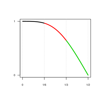
Figure 1: The function ${\rm q}:[0,1/2]\rightarrow[0,1]$ for $k=4$.

The function ${\rm q}$ is decreasing with ${\rm q}$, ${\rm q}^{\prime}$, ${\rm q}^{\prime\prime}$ ${\rm q}^{\prime\prime\prime}$ continuous. It was calculated by solving 8 equations with 8 unknowns, following the description in Subsection 3.3.1. We can now reason as in Subsection 3.3.4 to obtain for $\lambda$ satisfying (8) the bound (3) for the effective sparsity where $c_{k}$ and $C_{k}$ are appropriate constants.

3.4 Proof of Theorem 1.1

Taking $\bar{\mathcal{N}}_{-S}$ as the direct product of $\mathcal{N}_{-S}$ and an appropriate space spanned by $(k-1)s$ additional variables, we derived in Subsection 3.1.1 a bound for the length of the columns of the dictionary $\Psi^{-S}$. With these, we saw that the requirement (6) for $\lambda$ can is true when (8) holds. Then in Subsections 3.3.2, 3.3.3, 3.3.4 and 3.3.5 we derived a bound for the effective sparsity $\Gamma(q_{S},w_{-S})$ when (8) is strengthened to (10). Theorem 1.1 thus follows from the adaptive bound in Theorem 2.2 for the general analysis problem. $\sqcup\mkern-12.0mu\sqcap$

4 Conclusion

The sharp oracle inequalities with fast rates show that for $k\in\{1,2,3,4\}$ the estimator adapts to the unknown number of jumps in the $(k-1)^{\text{th}}$ discrete derivative and provide finite-sample prediction bounds. In particular, these show that the prediction error of the total variation regularized estimator is upper bounded by the optimal trade-off between approximation error and estimation error. The key tool for providing these results is bounding the effective sparsity using interpolating vectors. This approach allows extension to other problems as well, for instance higher dimensional extensions. See Ortelli and van de Geer (2019) where the Hardy-Krause variation serves as regularizer. For total variation on graphs, one may apply the fact that the dictionary can be formed by counting the number of times an edge is used when traveling from a given node to all other nodes. This can then be done on the sub-graphs formed by removing the active edges. For graphs with cycles there are several paths from one node to another. One may then choose those that allow for a smooth interpolating vector. Finally, the approach can be extended to estimation problems with $\ell_{1}$-penalty on the discrete derivative but loss functions other than least squares (see van de Geer (2020) for the case of logistic loss with total variation penalty on the canonical parameter).

Acknowledgements. We acknowledge support for this project from the the Swiss National Science Foundation (SNF grant 200020_169011). We thank the Associate Editor and two Referees for their very helpful remarks.

Appendix A Proof of Theorem 2.2

Let $\epsilon:=Y-f_{0}$ be the noise vector. The proof of oracle inequalities starts from the following basic inequality.

Lemma A.1 (Basic inequality)

For all $f\in\mathbb{R}^{n}$ it holds that

$$\lVert\hat{f}-f^{0}\rVert^{2}_{n}+\lVert\hat{f}-f\rVert^{2}_{n}\leq\lVert f-f^{0}\rVert^{2}_{n}+\frac{2\epsilon^{\prime}(\hat{f}-f)}{n}+2\lambda(\lVert Df\rVert_{1}-\lVert D\hat{f}\rVert_{1}).$$

Proof.

See Lemma B.1 in Ortelli and van de Geer [2020]. ∎

To derive oracle results from the basic inequality, we have to control the increments of the empirical process given by ${\epsilon^{\prime}(\hat{f}-f)}/{n}$. Inspired by Dalalyan et al. [2017], we decompose the increments of the empirical process into a part projected onto $\bar{\mathcal{N}}_{-S}$ and a remainder. For $f\in\mathbb{R}^{n}$ we let $w_{-S}(Df)_{-S}:=\{w_{j}(Df)_{j}\}_{j\notin\mathcal{D}\backslash S}$.

Lemma A.2 (Bound on the empirical process with mock variables.)

Choose $\lambda$ such that (6) holds and let $w_{-S}$ be as in Definition 2.1. Let $v>0$. It holds that with probability at least $1-e^{-u}-e^{-v}$,

$$\frac{\epsilon^{\prime}f}{n}\leq\left(\mathchoice{{\hbox{$\displaystyle\sqrt{\frac{\bar{r}_{S}}{n}\,}$}\lower 0.4pt\hbox{\vrule height=9.74387pt,depth=-7.79514pt}}}{{\hbox{$\textstyle\sqrt{\frac{\bar{r}_{S}}{n}\,}$}\lower 0.4pt\hbox{\vrule height=8.55138pt,depth=-6.84114pt}}}{{\hbox{$\scriptstyle\sqrt{\frac{\bar{r}_{S}}{n}\,}$}\lower 0.4pt\hbox{\vrule height=8.12082pt,depth=-6.49669pt}}}{{\hbox{$\scriptscriptstyle\sqrt{\frac{\bar{r}_{S}}{n}\,}$}\lower 0.4pt\hbox{\vrule height=8.12082pt,depth=-6.49669pt}}}+\mathchoice{{\hbox{$\displaystyle\sqrt{\frac{2v}{n}\,}$}\lower 0.4pt\hbox{\vrule height=8.59721pt,depth=-6.8778pt}}}{{\hbox{$\textstyle\sqrt{\frac{2v}{n}\,}$}\lower 0.4pt\hbox{\vrule height=6.01805pt,depth=-4.81447pt}}}{{\hbox{$\scriptstyle\sqrt{\frac{2v}{n}\,}$}\lower 0.4pt\hbox{\vrule height=4.2986pt,depth=-3.4389pt}}}{{\hbox{$\scriptscriptstyle\sqrt{\frac{2v}{n}\,}$}\lower 0.4pt\hbox{\vrule height=4.2986pt,depth=-3.4389pt}}}\right)\lVert f\rVert_{n}+\lambda\lVert w_{-S}(Df)_{-S}\rVert_{1},\ \forall f\in\mathbb{R}^{n}.$$

Proof of Lemma A.2.

We decompose the empirical process as

$$\epsilon^{\prime}f/{n}=\epsilon^{\prime}f_{\bar{\mathcal{N}}_{-S}}/{n}+{\epsilon^{\prime}f_{\bar{\mathcal{N}}_{-S}^{\perp}}}/{n}.$$

• For $v>0$ define the set

  $$\mathcal{V}:=\left\{\lVert\epsilon_{\bar{\mathcal{N}}_{-S}}\rVert_{n}\leq\mathchoice{{\hbox{$\displaystyle\sqrt{\frac{\bar{r}_{S}}{n}\,}$}\lower 0.4pt\hbox{\vrule height=9.74387pt,depth=-7.79514pt}}}{{\hbox{$\textstyle\sqrt{\frac{\bar{r}_{S}}{n}\,}$}\lower 0.4pt\hbox{\vrule height=8.55138pt,depth=-6.84114pt}}}{{\hbox{$\scriptstyle\sqrt{\frac{\bar{r}_{S}}{n}\,}$}\lower 0.4pt\hbox{\vrule height=8.12082pt,depth=-6.49669pt}}}{{\hbox{$\scriptscriptstyle\sqrt{\frac{\bar{r}_{S}}{n}\,}$}\lower 0.4pt\hbox{\vrule height=8.12082pt,depth=-6.49669pt}}}+\mathchoice{{\hbox{$\displaystyle\sqrt{\frac{2v}{n}\,}$}\lower 0.4pt\hbox{\vrule height=8.59721pt,depth=-6.8778pt}}}{{\hbox{$\textstyle\sqrt{\frac{2v}{n}\,}$}\lower 0.4pt\hbox{\vrule height=6.01805pt,depth=-4.81447pt}}}{{\hbox{$\scriptstyle\sqrt{\frac{2v}{n}\,}$}\lower 0.4pt\hbox{\vrule height=4.2986pt,depth=-3.4389pt}}}{{\hbox{$\scriptscriptstyle\sqrt{\frac{2v}{n}\,}$}\lower 0.4pt\hbox{\vrule height=4.2986pt,depth=-3.4389pt}}}\right\}.$$

  By applying Lemma 1 in Laurent and Massart [2000] (Lemma 8.6 in van de Geer [2016], a concentration inequality for $\chi^{2}$ random variables) to $\mathcal{V}$ we get that $\mathbb{P}(\mathcal{V})\geq 1-e^{-v}$.

  On $\mathcal{V}$ we have that

  $$\frac{\epsilon^{\prime}f_{\bar{\mathcal{N}}_{-S}}}{n}\leq\lVert\epsilon_{\bar{\mathcal{N}}_{-S}}\rVert_{n}\lVert\bar{f}_{\mathcal{N}_{-S}}\rVert_{n}\leq\left(\mathchoice{{\hbox{$\displaystyle\sqrt{\frac{\bar{r}_{S}}{n}\,}$}\lower 0.4pt\hbox{\vrule height=9.74387pt,depth=-7.79514pt}}}{{\hbox{$\textstyle\sqrt{\frac{\bar{r}_{S}}{n}\,}$}\lower 0.4pt\hbox{\vrule height=8.55138pt,depth=-6.84114pt}}}{{\hbox{$\scriptstyle\sqrt{\frac{\bar{r}_{S}}{n}\,}$}\lower 0.4pt\hbox{\vrule height=8.12082pt,depth=-6.49669pt}}}{{\hbox{$\scriptscriptstyle\sqrt{\frac{\bar{r}_{S}}{n}\,}$}\lower 0.4pt\hbox{\vrule height=8.12082pt,depth=-6.49669pt}}}+\mathchoice{{\hbox{$\displaystyle\sqrt{\frac{2v}{n}\,}$}\lower 0.4pt\hbox{\vrule height=8.59721pt,depth=-6.8778pt}}}{{\hbox{$\textstyle\sqrt{\frac{2v}{n}\,}$}\lower 0.4pt\hbox{\vrule height=6.01805pt,depth=-4.81447pt}}}{{\hbox{$\scriptstyle\sqrt{\frac{2v}{n}\,}$}\lower 0.4pt\hbox{\vrule height=4.2986pt,depth=-3.4389pt}}}{{\hbox{$\scriptscriptstyle\sqrt{\frac{2v}{n}\,}$}\lower 0.4pt\hbox{\vrule height=4.2986pt,depth=-3.4389pt}}}\right)\lVert f\rVert_{n}.$$

• For $\lambda_{0}(u)=\mathchoice{{\hbox{$\displaystyle\sqrt{(2\log(2(m-s))+2u)/n\,}$}\lower 0.4pt\hbox{\vrule height=7.5pt,depth=-6.00003pt}}}{{\hbox{$\textstyle\sqrt{(2\log(2(m-s))+2u)/n\,}$}\lower 0.4pt\hbox{\vrule height=7.5pt,depth=-6.00003pt}}}{{\hbox{$\scriptstyle\sqrt{(2\log(2(m-s))+2u)/n\,}$}\lower 0.4pt\hbox{\vrule height=5.25pt,depth=-4.20003pt}}}{{\hbox{$\scriptscriptstyle\sqrt{(2\log(2(m-s))+2u)/n\,}$}\lower 0.4pt\hbox{\vrule height=3.75pt,depth=-3.00002pt}}}$ defined as in (5) define the set

  $$\mathcal{U}:=\left\{\frac{\lvert\epsilon^{\prime}{\psi}_{j}^{-S}\rvert/n}{\lVert{\psi}_{j}^{-S}\rVert_{n}}\leq\lambda_{0}(u),\ \forall\ j\in\mathcal{D}\setminus\tilde{S}\right\}.$$

  We apply a standard concentration inequality for the maximum of $m-s$ standard Gaussian random variables (this can be found e.g. in Lemma 17.5 in van de Geer [2016]) to deduce that $\mathbb{P}(\mathcal{U})\geq 1-e^{-u}$.

  Since $f_{\bar{\mathcal{N}}_{-S}^{\perp}}=\Psi^{-S}(Df)_{-S}$ by the definition of the dictionary $\Psi^{-S}$, it holds on $\mathcal{U}$ that

  $${\epsilon^{\prime}f_{\bar{\mathcal{N}}_{-S}^{\perp}}}/{n}\leq\lambda\lVert{w}_{-{S}}(Df)_{-S}\rVert_{1}$$

  where

  $$w_{j}:=\|\psi_{j}^{-S}\|_{n}\lambda_{0}(u)/\lambda,\ j\in\mathcal{D}\backslash S.$$

The proof of the lemma is completed by noting that $\mathbb{P}(\mathcal{U}\cap\mathcal{V})\geq 1-e^{-u}-e^{-v}$. ∎

Lemma A.3 (A bound using $\Gamma^{2}(q_{S},w_{-S})$.)

Let $f\in\mathbb{R}^{n}$ and $S\subset\mathcal{D}$ be arbitrary, and $q_{S}:=\text{sign}(Df)_{S}$. Then for all $\tilde{f}\in\mathbb{R}^{n}$

$$\|(Df)_{S}\|_{1}-\|(D\tilde{f})_{S}\|_{1}-\|(1-w_{-S})(D(\tilde{f}-f))_{-S}\|_{1}\leq\Gamma(q_{S},w_{-S})\|f-\tilde{f}\|_{n}.$$

Proof.

Clearly $\|(Df)_{S}\|_{1}=q_{S}^{\prime}(Df)_{S}$. Moreover $\|(D\tilde{f})_{S}\|_{1}\geq q_{S}(D\tilde{f})_{S}$. Thus

$$\|(Df)_{S}\|_{1}-\|(D\tilde{f})_{S}\|_{1}\leq q_{S}^{\prime}(D(f-\tilde{f}))_{S}.$$

The result now follows from the Definition 2.1 of effective sparsity. ∎

Proof of Theorem 2.2.

By combining Lemma A.1 and Lemma A.2 we get that with probability at least $1-e^{-u}-e^{-v}$

$$\lVert\hat{f}-f^{0}\rVert^{2}_{n}+\lVert\hat{f}-f\rVert^{2}_{n} \leq \lVert f-f^{0}\rVert^{2}_{n}+2\left(\mathchoice{{\hbox{$\displaystyle\sqrt{\frac{\bar{r}_{S}}{n}\,}$}\lower 0.4pt\hbox{\vrule height=9.74387pt,depth=-7.79514pt}}}{{\hbox{$\textstyle\sqrt{\frac{\bar{r}_{S}}{n}\,}$}\lower 0.4pt\hbox{\vrule height=8.55138pt,depth=-6.84114pt}}}{{\hbox{$\scriptstyle\sqrt{\frac{\bar{r}_{S}}{n}\,}$}\lower 0.4pt\hbox{\vrule height=8.12082pt,depth=-6.49669pt}}}{{\hbox{$\scriptscriptstyle\sqrt{\frac{\bar{r}_{S}}{n}\,}$}\lower 0.4pt\hbox{\vrule height=8.12082pt,depth=-6.49669pt}}}+\mathchoice{{\hbox{$\displaystyle\sqrt{\frac{2v}{n}\,}$}\lower 0.4pt\hbox{\vrule height=8.59721pt,depth=-6.8778pt}}}{{\hbox{$\textstyle\sqrt{\frac{2v}{n}\,}$}\lower 0.4pt\hbox{\vrule height=6.01805pt,depth=-4.81447pt}}}{{\hbox{$\scriptstyle\sqrt{\frac{2v}{n}\,}$}\lower 0.4pt\hbox{\vrule height=4.2986pt,depth=-3.4389pt}}}{{\hbox{$\scriptscriptstyle\sqrt{\frac{2v}{n}\,}$}\lower 0.4pt\hbox{\vrule height=4.2986pt,depth=-3.4389pt}}}\right)\lVert\hat{f}-f\rVert_{n}$$

$$+ 2\lambda\lVert w_{-S}D(\hat{f}-f)_{-S}\rVert_{1}+2\lambda(\lVert Df\rVert_{1}-\lVert D\hat{f}\rVert_{1}).$$

The theorem we are proving has a non-adaptive bound and an adaptive one.
$\bullet$ For establishing the non-adaptive bound, we note that $\lVert w_{-S}\rVert_{\infty}\leq 1$, so that

$$\lVert w_{-S}(D(\hat{f}-f))_{-S}\rVert_{1}+\lVert Df\rVert_{1}-\lVert D\hat{f}\rVert_{1}\leq 2\|Df\|_{1}$$

and thus with probability at least $1-e^{-u}-e^{-v}$

$$\lVert\hat{f}-f^{0}\rVert^{2}_{n}+\lVert\hat{f}-f\rVert^{2}_{n} \leq \lVert f-f^{0}\rVert^{2}_{n}+2\left(\mathchoice{{\hbox{$\displaystyle\sqrt{\frac{\bar{r}_{S}}{n}\,}$}\lower 0.4pt\hbox{\vrule height=9.74387pt,depth=-7.79514pt}}}{{\hbox{$\textstyle\sqrt{\frac{\bar{r}_{S}}{n}\,}$}\lower 0.4pt\hbox{\vrule height=8.55138pt,depth=-6.84114pt}}}{{\hbox{$\scriptstyle\sqrt{\frac{\bar{r}_{S}}{n}\,}$}\lower 0.4pt\hbox{\vrule height=8.12082pt,depth=-6.49669pt}}}{{\hbox{$\scriptscriptstyle\sqrt{\frac{\bar{r}_{S}}{n}\,}$}\lower 0.4pt\hbox{\vrule height=8.12082pt,depth=-6.49669pt}}}+\mathchoice{{\hbox{$\displaystyle\sqrt{\frac{2v}{n}\,}$}\lower 0.4pt\hbox{\vrule height=8.59721pt,depth=-6.8778pt}}}{{\hbox{$\textstyle\sqrt{\frac{2v}{n}\,}$}\lower 0.4pt\hbox{\vrule height=6.01805pt,depth=-4.81447pt}}}{{\hbox{$\scriptstyle\sqrt{\frac{2v}{n}\,}$}\lower 0.4pt\hbox{\vrule height=4.2986pt,depth=-3.4389pt}}}{{\hbox{$\scriptscriptstyle\sqrt{\frac{2v}{n}\,}$}\lower 0.4pt\hbox{\vrule height=4.2986pt,depth=-3.4389pt}}}\right)\lVert\hat{f}-f\rVert_{n}$$

$$+ 4\lambda\lVert Df\rVert_{1}.$$

The non-adaptive bound therefore follows from the conjugate inequality $2ab\leq a^{2}+b^{2}$, $a,b\in\mathbb{R}$.
$\bullet$ For the adaptive bound we apply the inequalities

$$\lVert w_{-S}(D(\hat{f}-f))_{-S}\rVert_{1}+\lVert Df\rVert_{1}-\lVert D\hat{f}\rVert_{1}$$

$$\leq \|(1+w_{-S})(Df)_{-S}\|_{1}+\|(Df)_{S}\|_{1}-\|(Df)_{S}\|_{1}-\lVert(1-w_{-S})(D\hat{f})_{-S}\rVert_{1}$$

$$\leq 2\|(Df)_{-S}\|_{1}+\|(Df)_{S}\|_{1}-\|(D\hat{f})_{S}\|_{1}-\lVert(1-w_{-S})(D(\hat{f}-f))_{-S}\rVert_{1}.$$

Thus with probability at least $1-e^{-u}-e^{-v}$

$$\lVert\hat{f}-f^{0}\rVert^{2}_{n}+\lVert\hat{f}-f\rVert^{2}_{n}$$

$$\leq \lVert f-f^{0}\rVert^{2}_{n}+2\left(\mathchoice{{\hbox{$\displaystyle\sqrt{\frac{\bar{r}_{S}}{n}\,}$}\lower 0.4pt\hbox{\vrule height=9.74387pt,depth=-7.79514pt}}}{{\hbox{$\textstyle\sqrt{\frac{\bar{r}_{S}}{n}\,}$}\lower 0.4pt\hbox{\vrule height=8.55138pt,depth=-6.84114pt}}}{{\hbox{$\scriptstyle\sqrt{\frac{\bar{r}_{S}}{n}\,}$}\lower 0.4pt\hbox{\vrule height=8.12082pt,depth=-6.49669pt}}}{{\hbox{$\scriptscriptstyle\sqrt{\frac{\bar{r}_{S}}{n}\,}$}\lower 0.4pt\hbox{\vrule height=8.12082pt,depth=-6.49669pt}}}+\mathchoice{{\hbox{$\displaystyle\sqrt{\frac{2v}{n}\,}$}\lower 0.4pt\hbox{\vrule height=8.59721pt,depth=-6.8778pt}}}{{\hbox{$\textstyle\sqrt{\frac{2v}{n}\,}$}\lower 0.4pt\hbox{\vrule height=6.01805pt,depth=-4.81447pt}}}{{\hbox{$\scriptstyle\sqrt{\frac{2v}{n}\,}$}\lower 0.4pt\hbox{\vrule height=4.2986pt,depth=-3.4389pt}}}{{\hbox{$\scriptscriptstyle\sqrt{\frac{2v}{n}\,}$}\lower 0.4pt\hbox{\vrule height=4.2986pt,depth=-3.4389pt}}}+\right)\lVert\hat{f}-f\rVert_{n}+4\lambda\|(Df)_{-S}\|_{1}$$

$$+ 2\lambda\biggl{(}\|(Df)_{S}\|_{1}-\|(D\hat{f})_{S}\|_{1}-\lVert(1-w_{-S})(D(\hat{f}-f))_{-S}\rVert_{1}\biggr{)}$$

$$\leq \lVert f-f^{0}\rVert^{2}_{n}+2\left(\mathchoice{{\hbox{$\displaystyle\sqrt{\frac{\bar{r}_{S}}{n}\,}$}\lower 0.4pt\hbox{\vrule height=9.74387pt,depth=-7.79514pt}}}{{\hbox{$\textstyle\sqrt{\frac{\bar{r}_{S}}{n}\,}$}\lower 0.4pt\hbox{\vrule height=8.55138pt,depth=-6.84114pt}}}{{\hbox{$\scriptstyle\sqrt{\frac{\bar{r}_{S}}{n}\,}$}\lower 0.4pt\hbox{\vrule height=8.12082pt,depth=-6.49669pt}}}{{\hbox{$\scriptscriptstyle\sqrt{\frac{\bar{r}_{S}}{n}\,}$}\lower 0.4pt\hbox{\vrule height=8.12082pt,depth=-6.49669pt}}}+\mathchoice{{\hbox{$\displaystyle\sqrt{\frac{2v}{n}\,}$}\lower 0.4pt\hbox{\vrule height=8.59721pt,depth=-6.8778pt}}}{{\hbox{$\textstyle\sqrt{\frac{2v}{n}\,}$}\lower 0.4pt\hbox{\vrule height=6.01805pt,depth=-4.81447pt}}}{{\hbox{$\scriptstyle\sqrt{\frac{2v}{n}\,}$}\lower 0.4pt\hbox{\vrule height=4.2986pt,depth=-3.4389pt}}}{{\hbox{$\scriptscriptstyle\sqrt{\frac{2v}{n}\,}$}\lower 0.4pt\hbox{\vrule height=4.2986pt,depth=-3.4389pt}}}\right)\lVert\hat{f}-f\rVert_{n}+4\lambda\|(Df)_{-S}\|_{1}$$

$$+ 2\lambda\Gamma(q_{S},w_{-S})\|\hat{f}-f\|_{n}$$

where in the last inequality we used Lemma A.3. The proof is completed by applying again the conjugate inequality $2ab\leq a^{2}+b^{2}$, $a,b\in\mathbb{R}$. ∎

Appendix B Proofs for Section 3.1

B.1 Proof for the result in Subsection 3.1.1

Lemma B.1 (Symmetry of $\lVert{\psi}^{\mathcal{D}}_{j}\rVert_{2}$.)

Let $k\in[1:n-1]$ and $\Psi^{\cal D}=\Delta(k)^{+}$. For all $j\in\mathcal{D}$ we have that

$$\lVert\psi_{j}^{\mathcal{D}}\rVert^{2}_{2}=\lVert\psi_{n+k+1-j}^{\mathcal{D}}\rVert^{2}_{2}.$$

Proof of Lemma B.1.

$$\text{For }r=\{r_{i}\}_{i=1}^{n}=\begin{pmatrix}r_{1}\\ \vdots\\ r_{n}\end{pmatrix}\in\mathbb{R}^{n}\text{ define }\circlearrowright r=\{r_{i}\}_{i=n}^{1}=\begin{pmatrix}r_{n}\\ \vdots\\ r_{1}\end{pmatrix}.$$

Note that, for $r,\tilde{r}\in\mathbb{R}^{n}$ we have that $r^{\prime}\tilde{r}=(\circlearrowright r)^{\prime}\circlearrowright\tilde{r}$.

Since $\Delta(k)$ is of full rank, we have that ${\Delta(k)}^{+}={\Delta(k)}^{\prime}(\Delta(k){\Delta(k)}^{\prime})^{-1}.$

Let $r_{i}\in\mathbb{R}^{n-k}$ be the $i^{\text{th}}$ row of ${\Delta(k)}^{\prime}$, i.e. ${\Delta(k)}^{\prime}=\{r_{i}\}_{i=1}^{n}$. We observe that:

• For $k$ even, $r_{i}=\circlearrowright r_{n+1-i},\ i\in[n]$;

• For $k$ odd, $r_{i}=-\circlearrowright r_{n+1-i},\ i\in[n]$.

Define $P:=(\Delta(k){\Delta(k)}^{\prime})^{-1}\in\mathbb{R}^{(n-k)\times(n-k)}$ and let the rows and columns of $P$ be indexed by the set $\mathcal{D}=[n]\setminus[k]$. We have that $P$ is symmetric and all its diagonal entries are the same. Therefore, if we denote by $P_{j}$ the $j^{\text{th}}$ column of $P$, we note that $P_{j}=\circlearrowright P_{n+k+1-j},\ j\in\mathcal{D}$.

We distinguish two cases:

• When $k$ is even

  $$\psi_{n+k+1-j}^{\mathcal{D}} = \{r_{i}P_{n+k+1-j}\}_{i=1}^{n}=\{r_{i}\circlearrowright P_{j}\}_{i=1}^{n}=\{\circlearrowright r_{n+1-i}\circlearrowright P_{j}\}_{i=1}^{n}$$

  $$= \{r_{n+1-i}P_{j}\}_{i=1}^{n}=\{r_{i}P_{j}\}_{i=n}^{1}=\circlearrowright\{r_{i}P_{j}\}_{i=1}^{n}=\circlearrowright{\psi_{j}^{\mathcal{D}}}.$$

• When $k$ is odd, by similar calculations $\psi_{n+k+1-j}^{\mathcal{D}}=-\circlearrowright\psi_{j}^{\mathcal{D}}$.

Since, for $r\in\mathbb{R}^{n}$, $\lVert r\rVert^{2}_{2}=\lVert\pm\circlearrowright r\rVert^{2}_{2}$ we get the claim. ∎

To calculate the pseudo inverse of $\Delta(k)$ we proceed as follows (cf. Lemma 2.2 in Ortelli and van de Geer [2020]).

1. We select the matrix $A(k)\in\mathbb{R}^{k\times n}$, s.t.

   $$A(k)_{ij}=\begin{dcases}(-1)^{j+i}\binom{i}{j},&j=i-l,\ l\in\{0,\ldots,i-1\},\ i\in[k],\\ 0,&\text{else}.\end{dcases}$$

2. We find $X^{k}=\begin{pmatrix}A(k)\\ \Delta(k)\end{pmatrix}^{-1}\in\mathbb{R}^{n\times n}$. We have that $X^{k}=\{\phi^{k}_{j}\}_{j\in[n]}$, where

   • for $k=1$, $\phi^{1}_{j}=1_{\{i\geq j\}},\ i,\ j\in[n]$,

   • and for $k\geq 2$,

     $$\phi_{j}^{k}=\begin{dcases}\phi^{j}_{j},&1\leq j<k\\ \sum_{l\geq j}\phi_{l}^{k-1},&k\leq j\leq n.\end{dcases}$$

     This is the falling factorial basis for equidistant design, see Wang et al. [2014] and Tibshirani [2020]]. In the notation for the general analysis problem (see the beginning of Subsection 3.1) $\{\psi_{j}\}_{j=1}^{n}:=\{\phi_{j}^{k}\}_{j=1}^{n}$ is a complete dictionary.

3. Then $\Delta^{+}(k)=\{\psi_{j}^{\mathcal{D}}\}_{j\in[k+1:n]}$, where

   $$\psi_{j}^{\mathcal{D}}=({\phi}^{k}_{j})_{\mathcal{N}_{\mathcal{D}}^{\perp}},j\in[k+1:n].$$

Proof of Lemma 3.1.

We roughly estimate

$$\lVert\psi_{j}^{\mathcal{D}}\rVert_{2}^{2}\leq\lVert{\phi_{j}}^{k}\rVert_{2}^{2},\ ({n+k+1})/{2}\leq j\leq n,$$

where

$$\lVert{\phi_{j}}^{k}\rVert^{2}_{2}\leq\int_{0}^{n+1-j}x^{2k-2}dx\leq(n+1-j)^{2k-1}.$$

By symmetry (Lemma B.1), we obtain the claim. ∎

B.2 Proofs for the results in Subsection 3.1.3

Proof of Lemma 3.2.

Let $\psi_{1}:\equiv 1\in\mathbb{R}^{n}$ and

$$\psi_{j}:=\{(i-j+1)1_{\{i\geq j\}}\}_{i\in[1:n]},\ j\in[2:n].$$

We want to find the anti-projections of the vectors $\psi_{j},\ j\in[3:n]$ onto the linear space spanned by $\psi_{1}$ and $\psi_{2}$.

We use the Gram-Schmidt procedure to orthonormalize the basis on which we want to project.

By $u_{1},u_{2}$ we denote two vectors orthogonal to each other, which span the linear span of $\psi_{1},\ \psi_{2}$, and by $e_{1},e_{2}$ their normalized version. We take $u_{1}=\psi_{1}\equiv 1$. Then ${e_{1}=n^{-1/2}}$. We now take $u_{2}=\psi_{2}-\langle\psi_{2},e_{1}\rangle e_{1}$. We have that $\langle\psi_{2},e_{1}\rangle=\frac{n(n-1)}{2n^{1/2}}$ and thus $u_{2}=\left\{(i-1)1_{\{i\geq 2\}}-\frac{n-1}{2}\right\}_{i=1}^{n}$. The norm of $u_{2}$ is $\lVert u_{2}\rVert^{2}_{2}=\frac{(n+1)n(n-1)}{12}$ and it follows that

$$e_{2}=\mathchoice{{\hbox{$\displaystyle\sqrt{\frac{12}{(n+1)n(n-1)}\,}$}\lower 0.4pt\hbox{\vrule height=11.44444pt,depth=-9.1556pt}}}{{\hbox{$\textstyle\sqrt{\frac{12}{(n+1)n(n-1)}\,}$}\lower 0.4pt\hbox{\vrule height=8.01111pt,depth=-6.40892pt}}}{{\hbox{$\scriptstyle\sqrt{\frac{12}{(n+1)n(n-1)}\,}$}\lower 0.4pt\hbox{\vrule height=5.72221pt,depth=-4.57779pt}}}{{\hbox{$\scriptscriptstyle\sqrt{\frac{12}{(n+1)n(n-1)}\,}$}\lower 0.4pt\hbox{\vrule height=5.72221pt,depth=-4.57779pt}}}\left\{(i-1)1_{\{i\geq 2\}}-\frac{n-1}{2}\right\}_{i=1}^{n}.$$

Let $\bar{\psi}_{j}$ denote the projection of $\psi_{j}$ onto the linear span of $e_{1},\ e_{2}$ and let $\psi_{j}^{\mathcal{D}}=\psi_{j}-\bar{\psi}_{j}$ be denote the anti-projection. It holds that

$$\bar{\psi}_{j}=\langle\psi_{j},e_{1}\rangle e_{1}+\langle\psi_{j},e_{2}\rangle e_{2}\text{ and }\lVert\bar{\psi}_{j}\rVert^{2}_{2}=\langle\psi_{j},e_{1}\rangle^{2}+\langle\psi_{j},e_{2}\rangle^{2}.$$

Moreover by Pythagoras $\lVert\psi_{j}^{\mathcal{D}}\rVert^{2}_{2}=\lVert\psi_{j}\rVert^{2}_{2}-\lVert\bar{\psi}_{j}\rVert^{2}_{2}$.

To compute the length of the anti-projections we thus have to compute the coefficients of the projections onto the orthonormal vectors spanning the linear space we project onto (i.e. $\langle\psi_{j},e_{1}\rangle$ and $\langle\psi_{j},e_{2}\rangle$) and the lengths of the vectors to project (i.e. $\lVert\psi_{j}\rVert^{2}_{2}$).

We omit all the steps of the computations, which were performed with the support of the software “Wolfram Mathematica 11”. We present directly the results, that for the inner products $\langle\psi_{j},e_{1}\rangle$ and $\langle\psi_{j},e_{2}\rangle$ are

$$\langle\psi_{j},e_{1}\rangle=\frac{(n-j+1)(n-j+2)}{2\mathchoice{{\hbox{$\displaystyle\sqrt{n\,}$}\lower 0.4pt\hbox{\vrule height=4.30554pt,depth=-3.44446pt}}}{{\hbox{$\textstyle\sqrt{n\,}$}\lower 0.4pt\hbox{\vrule height=4.30554pt,depth=-3.44446pt}}}{{\hbox{$\scriptstyle\sqrt{n\,}$}\lower 0.4pt\hbox{\vrule height=3.01389pt,depth=-2.41113pt}}}{{\hbox{$\scriptscriptstyle\sqrt{n\,}$}\lower 0.4pt\hbox{\vrule height=2.15277pt,depth=-1.72223pt}}}},$$

$$\langle\psi_{j},e_{2}\rangle=\mathchoice{{\hbox{$\displaystyle\sqrt{\frac{1}{12(n+1)n(n-1)}\,}$}\lower 0.4pt\hbox{\vrule height=11.44444pt,depth=-9.1556pt}}}{{\hbox{$\textstyle\sqrt{\frac{1}{12(n+1)n(n-1)}\,}$}\lower 0.4pt\hbox{\vrule height=8.01111pt,depth=-6.40892pt}}}{{\hbox{$\scriptstyle\sqrt{\frac{1}{12(n+1)n(n-1)}\,}$}\lower 0.4pt\hbox{\vrule height=5.72221pt,depth=-4.57779pt}}}{{\hbox{$\scriptscriptstyle\sqrt{\frac{1}{12(n+1)n(n-1)}\,}$}\lower 0.4pt\hbox{\vrule height=5.72221pt,depth=-4.57779pt}}}(n-j+1)(n-j+2)(n+2j-3).$$

The length of the vectors to project is given by

$$\lVert\psi_{j}\rVert_{2}^{2}=\frac{(n-j+1)(n-j+2)(2n-2j+3)}{6}.$$

For the length of the projections we obtain the expression

$$\lVert\bar{\psi_{j}}\rVert^{2}_{2}=\frac{(n-j+1)^{2}(n-j+2)^{2}}{4n}\left(1+\frac{(n+2j-3)^{2}}{3(n-1)(n+1)}\right).$$

For the length of the anti-projections we obtain the exact expression

$$\lVert\psi_{j}^{\mathcal{D}}\rVert^{2}_{2}=\frac{(n-j+1)(n-j+2)(j-2)(j-1)(2j(n-j+3)-3(n+1))}{6n(n+1)(n-1)}.$$

∎

B.3 Proof for the result in Subsection 3.1.4

Proof of Lemma 3.3.

Let $\psi_{1}:\equiv 1$, $\psi_{2}:=\left\{i-1\right\}_{i\in[1:n]}$,

$$\psi_{j}:=\left\{(i-j+1)(i-j+2)1_{\{i\geq j\}}/2\right\}_{i\in[1:n]},\ j\in[2:n].$$

The length of the anti-projections is given by

$$\lVert\psi_{j}^{\mathcal{D}}\rVert^{2}_{2}=\lVert\psi_{j}\rVert^{2}_{2}-\langle\psi_{j},e_{1}\rangle^{2}-\langle\psi_{j},e_{2}\rangle^{2}-\langle\psi_{j},e_{3}\rangle^{2}.$$

The orthonormal basis vectors $e_{1}$ and $e_{2}$ are the same as in the proof of Lemma 3.2. Here as well the computations have been dome with the support of the software “Wolfram Mathematica 11”. In a first step we want to find

$$u_{3}=\psi_{3}-\langle\psi_{3},e_{1}\rangle e_{1}-\langle\psi_{3},e_{2}\rangle e_{2}$$

and its normalized version $e_{3}=u_{3}/\lVert u_{3}\rVert_{2}$.

We use the Gram-Schmidt process. We have that

$$\lVert\psi_{j}\rVert^{2}_{2}=\sum_{i=1}^{n}1_{\{i\geq j\}}\frac{(i-j+1)^{2}(i-j+2)^{2}}{4}$$

$$= \frac{(n+3-j)(n+2-j)(n+1-j)(10-12j+3j^{2}+12n-6jn+3n^{2})}{60}.$$

Moreover, for the coefficients of the projections onto $e_{1}$ we have

$$\langle\psi_{j},e_{1}\rangle=\frac{(n+3-j)(n+2-j)(n+1-j)}{6\mathchoice{{\hbox{$\displaystyle\sqrt{n\,}$}\lower 0.4pt\hbox{\vrule height=4.30554pt,depth=-3.44446pt}}}{{\hbox{$\textstyle\sqrt{n\,}$}\lower 0.4pt\hbox{\vrule height=4.30554pt,depth=-3.44446pt}}}{{\hbox{$\scriptstyle\sqrt{n\,}$}\lower 0.4pt\hbox{\vrule height=3.01389pt,depth=-2.41113pt}}}{{\hbox{$\scriptscriptstyle\sqrt{n\,}$}\lower 0.4pt\hbox{\vrule height=2.15277pt,depth=-1.72223pt}}}}.$$

For the coefficients of the projections onto $e_{2}$ we have that

$$\langle\psi_{j},e_{2}\rangle=\frac{(n+3-j)(n+2-j)(n+1-j)(n+j-2)}{\mathchoice{{\hbox{$\displaystyle\sqrt{48(n+1)n(n-1)\,}$}\lower 0.4pt\hbox{\vrule height=7.5pt,depth=-6.00003pt}}}{{\hbox{$\textstyle\sqrt{48(n+1)n(n-1)\,}$}\lower 0.4pt\hbox{\vrule height=7.5pt,depth=-6.00003pt}}}{{\hbox{$\scriptstyle\sqrt{48(n+1)n(n-1)\,}$}\lower 0.4pt\hbox{\vrule height=5.25pt,depth=-4.20003pt}}}{{\hbox{$\scriptscriptstyle\sqrt{48(n+1)n(n-1)\,}$}\lower 0.4pt\hbox{\vrule height=3.75pt,depth=-3.00002pt}}}}.$$

We thus obtain that the anti-projection of $\psi_{3}$ onto $\text{span}(\psi_{1},\psi_{2})$ is given by

$$u_{3}=\psi_{3}-\langle\psi_{3},e_{1}\rangle e_{1}-\langle\psi_{3},e_{2}\rangle e_{2}=\left\{\frac{(i-1)(i-n)}{2}+\frac{(n-1)(n-2)}{12}\right\}_{i=1}^{n}.$$

The $\ell_{2}$-norm of $u_{3}$ is

$$\lVert u_{3}\rVert^{2}_{2}=\frac{(n+2)(n+1)n(n-1)(n-2)}{720}$$

and the third vector $e_{3}$ of the orthonormal basis writes as

$$e_{3}=u_{3}/\lVert u_{3}\rVert_{2}$$

$$= \mathchoice{{\hbox{$\displaystyle\sqrt{\frac{720}{(n^{2}-4)(n^{2}-1)n}\,}$}\lower 0.4pt\hbox{\vrule height=11.44444pt,depth=-9.1556pt}}}{{\hbox{$\textstyle\sqrt{\frac{720}{(n^{2}-4)(n^{2}-1)n}\,}$}\lower 0.4pt\hbox{\vrule height=8.01111pt,depth=-6.40892pt}}}{{\hbox{$\scriptstyle\sqrt{\frac{720}{(n^{2}-4)(n^{2}-1)n}\,}$}\lower 0.4pt\hbox{\vrule height=5.72221pt,depth=-4.57779pt}}}{{\hbox{$\scriptscriptstyle\sqrt{\frac{720}{(n^{2}-4)(n^{2}-1)n}\,}$}\lower 0.4pt\hbox{\vrule height=5.72221pt,depth=-4.57779pt}}}\left\{\frac{(i-1)(i-n)}{2}+\frac{(n-1)(n-2)}{12}\right\}_{i=1}^{n}.$$

We can now compute the coefficient of the projections of $\psi_{j}$ onto $e_{3}$:

$$\langle\psi_{j},e_{3}\rangle=$$

$$\frac{(n+3-j)(n+2-j)(n+1-j)(6j^{2}+3jn-24j+n^{2}-6n+20)}{\mathchoice{{\hbox{$\displaystyle\sqrt{720(n+2)(n+1)n(n-1)(n-2)\,}$}\lower 0.4pt\hbox{\vrule height=7.5pt,depth=-6.00003pt}}}{{\hbox{$\textstyle\sqrt{720(n+2)(n+1)n(n-1)(n-2)\,}$}\lower 0.4pt\hbox{\vrule height=7.5pt,depth=-6.00003pt}}}{{\hbox{$\scriptstyle\sqrt{720(n+2)(n+1)n(n-1)(n-2)\,}$}\lower 0.4pt\hbox{\vrule height=5.25pt,depth=-4.20003pt}}}{{\hbox{$\scriptscriptstyle\sqrt{720(n+2)(n+1)n(n-1)(n-2)\,}$}\lower 0.4pt\hbox{\vrule height=3.75pt,depth=-3.00002pt}}}}.$$

Combining the formulas for the quantities we found, we get the claim. ∎

Appendix C Proofs for Section 3.3

C.1 Proof for the result in Subsection 3.3.1

Proof of Lemma 3.6.

We have for $j\geq k$

$$\Delta(k)j^{2k-1\over 2} = \sum_{l=0}^{k}{k\choose l}(-1)^{l}(j-l)^{2k-1\over 2}$$

$$= j^{2k-1\over 2}\biggl{[}\sum_{l=0}^{k}{k\choose l}(-1)^{l}\biggl{(}1-{l\over j}\biggr{)}^{2k-1\over 2}\biggr{]}.$$

We do a $(k-1)$-term Taylor expansion of $x\mapsto(1-x)^{2k-1\over 2}$ around $x=0$:

$$(1-x)^{2k-1\over 2}=\sum_{i=0}^{k-1}a_{i}x^{i}+{\rm rem}(x),$$

where $a_{0}=1$, $a_{1}=-{2k-1\over 2},\cdots$ are the coefficients of the Taylor expansion and where the remainder ${\rm rem}(x)$ satisfies for some constant ${\rm C}_{k}$

$$\sup_{0\leq x\leq 1/2}|{\rm rem}(x)|\leq{\rm C}_{k}|x|^{k}.$$

Thus

$$\sum_{l=0}^{k}{k\choose l}(-1)^{l}\biggl{(}1-{l\over j}\biggr{)}^{2k-1\over 2}$$

$$= \sum_{l=0}^{k}{k\choose l}(-1)^{l}\sum_{{\rm k}=0}^{k-1}a_{i}\biggl{(}{l\over j}\biggr{)}^{i}+\sum_{l=0}^{k}{k\choose l}(-1)^{l}{\rm rem}\biggl{(}{l\over j}\biggr{)}$$

$$= \underbrace{\Delta(k){\bf p}}_{=0}+\sum_{l=0}^{k}{k\choose l}(-1)^{l}{\rm rem}\biggl{(}{l\over j}\biggr{)},$$

where

$${\bf p}=\biggl{\{}(-1)^{k}\sum_{i=0}^{k-1}{a_{i}}\biggl{(}{l\over j}\biggr{)}^{i}\biggr{\}}_{l=0,\ldots,k-1}$$

is a polynomial of degree $k-1$ and hence $\Delta(k){\rm p}=0$. It follows that for $j\geq 2k$,

$$\biggl{|}\sum_{l=0}^{k}{k\choose l}(-1)^{l}\biggl{(}1-{l\over j}\biggr{)}^{2k-1\over 2}\biggr{|}\leq\sum_{l=0}^{k}{k\choose l}\biggl{|}{\rm rem}\biggl{(}{l\over j}\biggr{)}\biggr{|}\leq\tilde{\rm C}_{k}{1\over j^{k}}.$$

But then for $j\geq 2k$

$$\Delta(k)j^{2k-1\over 2}\leq\tilde{\rm C}_{k}{1\over\mathchoice{{\hbox{$\displaystyle\sqrt{j\,}$}\lower 0.4pt\hbox{\vrule height=6.59525pt,depth=-5.27623pt}}}{{\hbox{$\textstyle\sqrt{j\,}$}\lower 0.4pt\hbox{\vrule height=6.59525pt,depth=-5.27623pt}}}{{\hbox{$\scriptstyle\sqrt{j\,}$}\lower 0.4pt\hbox{\vrule height=4.61667pt,depth=-3.69336pt}}}{{\hbox{$\scriptscriptstyle\sqrt{j\,}$}\lower 0.4pt\hbox{\vrule height=3.29762pt,depth=-2.63812pt}}}}.$$

So

$$\sum_{j=2k}^{d}|\Delta(k)j^{2k-1\over 2}|^{2}\leq\tilde{\rm C}_{k}^{2}(1+\log d).$$

Finally, for $k\leq j<2k$,

$$\Delta(k)j^{2k-1\over 2}\leq j^{2k-1\over 2}\sum_{l=0}^{k}{k\choose l}\leq 2^{k}k^{2k-1\over 2}.$$

Thus

$$\sum_{j=k}^{d}|\Delta(k)j^{2k-1\over 2}|^{2}\leq(2k)^{2k}+\tilde{\rm C}_{k}^{2}(1+\log d)\leq\tilde{C}_{k}^{2}(1+\log d)$$

for some constant $\tilde{C}_{k}$. ∎

C.2 Proof of the result in Subsection 3.3.4

Proof of Lemma 3.7.

First

$$\Delta(2){\bf q}_{d+2} = -{\bar{a}_{0}[\Delta(2)(d+2)^{5/2}]\over d^{5/2}}=-{\bar{a}_{0}\alpha_{2}\over d^{2}}$$

$$= -{1\over d^{2}}{\alpha_{2}\gamma_{2}\over\gamma_{2}-\alpha_{2}+(\gamma_{1}\alpha_{2}+\alpha_{1}\gamma_{2})}$$

$$\Delta(2){\bf p}_{d+2} = -{\bar{a}_{3}[\Delta(2)d^{3}]\over d^{3}}=-{\bar{a}_{3}\gamma_{2}\over d^{2}}=-{1\over d^{2}}{\alpha_{2}\gamma_{2}\over\gamma_{2}-\alpha_{2}+(\gamma_{1}\alpha_{2}-\alpha_{1}\gamma_{2})}\ .$$

Second

$$\Delta{\bf q}_{d+1} = -{\bar{a}_{0}[\Delta(d+1)^{5/2}]\over d^{5/2}}=-{\bar{a}_{0}\alpha_{1}\over d}=-{1\over d}{\gamma_{2}\alpha_{1}\over\gamma_{2}-\alpha_{2}+(\gamma_{1}\alpha_{2}+\alpha_{1}\gamma_{2})}$$

$$\Delta{\bf p}_{d+1} = {\bar{a}_{3}[\Delta d^{3}]\over d^{3}}-{\bar{a}_{1}\over d}={\bar{a}_{3}\gamma_{1}\over d}-{\bar{a}_{1}\over d}$$

$$= {1\over d}{\alpha_{2}\gamma_{1}-(\gamma_{1}\alpha_{2}+\alpha_{1}\gamma_{2})\over\gamma_{2}-\alpha_{2}+(\gamma_{1}\alpha_{2}+\alpha_{1}\gamma_{2})}=-{1\over d}{\alpha_{1}\gamma_{2}\over\gamma_{2}-\alpha_{2}+(\gamma_{1}\alpha_{2}+\alpha_{1}\gamma_{2})}\ .$$

Finally

$${\bf q}_{d} = 1-{\bar{a}_{0}}=1-{\gamma_{2}\over\gamma_{2}-\alpha_{2}+(\gamma_{1}\alpha_{2}+\alpha_{1}\gamma_{2})}$$

$$= {\gamma_{1}\alpha_{2}+\alpha_{1}\gamma_{2}-\alpha_{2}\over\gamma_{2}-\alpha_{2}+(\gamma_{1}\alpha_{2}+\alpha_{1}\gamma_{2})}$$

$${\bf p}_{d} = -\bar{a}_{3}+\bar{a}_{1}={\gamma_{1}\alpha_{2}+\alpha_{1}\gamma_{2}-\alpha_{2}\over\gamma_{2}-\alpha_{2}+(\gamma_{1}\alpha_{2}+\alpha_{1}\gamma_{2})}\ .$$

∎

References

- Belloni et al. [2011] Alexandre Belloni, Victor Chernozhukov, and Lie Wang. Square-root lasso: pivotal recovery of sparse signals via conic programming. Biometrika, 98(4):791–806, 2011.
- Boyer et al. [2017] Claire Boyer, Yohann De Castro, and Joseph Salmon. Adapting to unknown noise level in sparse deconvolution. Information and Inference: A Journal of the IMA, 6(3):310–348, 2017.
- Candès and Fernandez-Granda [2014] Emmanuel Candès and Carlos Fernandez-Granda. Towards a mathematical theory of super-resolution. Communications on Pure and Applied Mathematics, 67(6):906–956, 2014.
- Candès and Plan [2011] Emmanuel Candès and Yaniv Plan. A probabilistic and RIPless theory of compressed sensing. IEEE Transactions on Information Theory, 57(11):7235–7254, 2011.
- Chatterjee and Goswami [2019] Sabyasachi Chatterjee and Subhajit Goswami. Adaptive estimation of multivariate piecewise polynomials and bounded variation functions by optimal decision trees. arXiv preprint arXiv:1911.11562, 2019.
- Dalalyan et al. [2017] Arnak Dalalyan, Mohamed Hebiri, and Johannes Lederer. On the prediction performance of the lasso. Bernoulli, 23(1):552–581, 2017.
- Donoho and Johnstone [1998] David Donoho and Iain Johnstone. Minimax estimation via wavelet shrinkage. Annals of Statistics, 26(3):879–921, 1998.
- Elad et al. [2007] Michael Elad, Peyman Milanfar, and Ron Rubinstein. Analysis versus synthesis in signal priors. Inverse Problems, 23(947), 2007.
- Guntuboyina et al. [2020] Adityanand Guntuboyina, Donovan Lieu, Sabayasachi Chatterjee, and Bodhisattva Sen. Adaptive risk bounds in univariate total variation denoising and trend filtering. Annals of Statistics, 48(1):205–229, 2020.
- Kim et al. [2009] Seung-Jean Kim, Kwangmoo Koh, Stephen Boyd, and Dimitry Gorinevsky. trend filtering. SIAM review, 51(2):339–360, 2009.
- Laurent and Massart [2000] Béarice Laurent and Pascal Massart. Adaptive estimation of a quadratic functional by model selection. Annals of Statistics, 28(5):1302–1338, 2000.
- Mammen and van de Geer [1997] Enno Mammen and Sara van de Geer. Locally adaptive regression splines. Annals of Statistics, 25(1):387–413, 1997.
- Ortelli and van de Geer [2019] Francesco Ortelli and Sara van de Geer. Oracle inequalities for image denoising with total variation regularization. arXiv preprint arXiv:1911.07231, 2019.
- Ortelli and van de Geer [2020] Francesco Ortelli and Sara van de Geer. Oracle inequalities for square root analysis estimators with application to total variation penalties. Information and Inference: A Journal of the IMA, (iaaa002), 2020.
- Qian and Jia [2016] Junyang Qian and Jinzhu Jia. On stepwise pattern recovery of the fused Lasso. Computational Statistics and Data Analysis, 94:221–237, 2016.
- Rudin et al. [1992] Leonid Rudin, Stanley Osher, and Emad Fatemi. Nonlinear total variation based noise removal algorithms. Physica D, 60:259–268, 1992.
- Sadhanala and Tibshirani [2017] Veeranjaneyulu Sadhanala and Ryan J Tibshirani. Additive Models with Trend Filtering. arXiv:1702.05037v4, 2017.
- Sadhanala et al. [2017] Veeranjaneyulu Sadhanala, Yu-Xiang Wang, James Sharpnack, and Ryan Tibshirani. Higher-order total variation classes on grids: Minimax theory and trend filtering methods. In Advances in Neural Information Processing Systems, pages 5800–5810, 2017.
- Steidl et al. [2006] Gabriele Steidl, Stephan Didas, and Julia Neumann. Splines in higher order TV regularization. International Journal of Computer Vision, 70(3):241–255, 2006.
- Tang et al. [2014] Gongguo Tang, Badri Narayan Bhaskar, and Benjamin Recht. Near minimax line spectral estimation. IEEE Transactions on Information Theory, 61(1):499–512, 2014.
- Tibshirani [1996] Robert Tibshirani. Regression Shrinkage and Selection via the Lasso. J. R. Statist. Soc. B, 58(1):267–288, 1996.
- Tibshirani [2014] Ryan Tibshirani. Adaptive piecewise polynomial estimation via trend filtering. Annals of Statistics, 42(1):285–323, 2014.
- Tibshirani [2020] Ryan Tibshirani. Divided differences, falling factorials, and discrete splines: Another look at trend filtering and related problems. arXiv preprint arXiv:2003.03886, 2020.
- van de Geer [2016] Sara van de Geer. Estimation and Testing under Sparsity, volume 2159. Springer, 2016.
- van de Geer [2020] Sara van de Geer. Logistic regression with total variation regularization. arXiv preprint arXiv:2003.02678, 2020. Tentatively accepted by Transactions of A. Razmadze Mathematical Institute.
- Wang et al. [2014] Yu-Xiang Wang, Alex Smola, and Ryan Tibshirani. The falling factorial basis and its statistical applications. In International Conference on Machine Learning, pages 730–738, 2014.
- Wang et al. [2016] Yu-Xiang Wang, James Sharpnack, Alex Smola, and Ryan Tibshirani. Trend filtering on graphs. Journal of Machine Learning Research, 17:15–147, 2016.