Splitting of nonlinear-Schrödinger breathers by linear and nonlinear localized potentials

Abstract

We consider evolution of one-dimensional nonlinear-Schrödinger (NLS) two-soliton complexes (breathers) with narrow repulsive or attractive potentials (barrier or well, respectively). By means of systematic simulations, we demonstrate that the breather may either split into constituent fundamental solitons (fragments) moving in opposite directions, or bounce as a whole from the barrier. A critical initial position of the breather, which separates these scenarios, is predicted by an analytical approximation. The narrow potential well tends to trap the fragment with the larger amplitude, while the other one escapes. The interaction of the breather with a nonlinear potential barrier is also considered. The ratio of amplitudes of the emerging free solitons may be different from the $3:1$ value suggested by the exact NLS solution, especially in the case of the nonlinear potential barrier. Post-splitting velocities of escaping solitons may be predicted by an approximation based on the energy balance.

I Introduction

It is commonly known that solitons, i.e., robust self-trapped modes in nonlinear media, are fundamental excitations, and in many cases represent ground states, in a broad variety of physical settings KA ; DP ; Y . Additional interest to solitons has been attracted by the creation of localized matter-wave states in Bose-Einstein condensates (BECs) of ultracold ${}^{7}\mathrm{Li}$ strecker2002 ; khaykovich2002 ; strecker2003 and ${}^{85}\mathrm{Rb}$ cornish2006 ; marchant2013 atoms. These solitons were produced in the quasi-one-dimensional (quasi-1D) form, by loading the atomic BEC into a strongly anisotropic (cigar-shaped) potential trap. The latter setting is accurately approximated, in the framework of the mean-field theory, by the Gross-Pitaevskii equations (GPEs) Pit . In the case of attractive interactions between atoms, the GPE, being similar to the integrable nonlinear Schrödinger (NLS) equation, gives rise to well-known soliton solutions zakharov1972 ; zakharov1984 ; satsuma1974 .

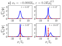
(a)

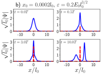
(b)

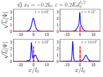
(c)

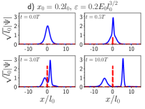
(d)

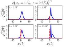
(e)

Figure 1: Snapshots of direct simulations of splitting of input (9) under the action of the the linear potential barrier with $\varepsilon=0.2$ in Eq. (1), and different values of shift $x_{0}$: a) $x_{0}=-0.0002$ b) $x_{0}=0.0002$; c) $x_{0}=-0.2$; d) $x_{0}=0.2$; e) $x_{0}=1.3$. The snapshots are displayed at times indicated in the panels. The blue solid lines represent profiles of $|\Psi(x)|$ at the respective moments of time, while the red dashed line is the shape of the splitting barrier. Panels a) and b) demonstrate that even an extremely small shift of the initial position of the input from the central point leads to strong (although slowly developing) breaking of the spatial symmetry and fission of the breather.

In this work we focus on two-soliton solutions, also known as breathers. Using the inverse-scattering-transform technique which applies to many integrable equations zakharov1972 ; zakharov1984 ; satsuma1974 , one can show that, in the simplest case the breather may be considered as a nonlinear superposition of two fundamental solitons, with the ratio of amplitudes $3:1$ and zero relative velocity (it is relevant to mention that the Lieb-Liniger model LLM ; LLM-review , i.e., the integrable quantum version of the NLS equation, does not produce spatially-localized solitons and breathers, supporting solely spatially-homogeneous strings of bound quantum particles Volodya ). Thus, it is reasonable to expect that perturbations, represented by additional terms in the NLS equation, which break its integrability, may split the breather into constituent solitons (fragments) HS-resonant ; Khaykovich ; dunjko2015 ; malomed2018 ; we .

In many physical settings, an important type of integrability-breaking perturbations added to the NLS equation is represented by narrow potential barriers barrier1 -barrier6 or wells well2 ; well1 . In this work we aim to consider the interaction of two-soliton breathers with a narrow linear barrier and well, as well as with a nonlinear barrier. This setting directly represents experimentally relevant situations. In optics, a light beam in the form of the spatial two-soliton can propagate along the medium’s defect in the form of the barrier or well. In a BEC, a breather traveling in a cigar-shaped trap can hit a splitting barrier, which is a typical situation in matter-wave interferometers interferometer1 -interferometer7 . The interaction with localized barriers and wells was considered many times for fundamental solitons barrier1 -HS , but it was not previously studied for breathers. In particular, because splitting an incident fundamental soliton in two fragments by a barrier underlies the operation of matter-wave interferometers, it is definitely relevant to consider a similar effect for two-soliton breathers, for which the splitting is a much more natural, hence also more controllable, outcome of the interaction with the localized potential.

The breather-barrier interaction is controlled by two main parameters: the barrier’s height and its initial shift with respect to the breather’s center. By means of systematic simulations, we explore the outcome of the interaction, in the parameter space of the model. The results make it possible to identify two distinct regimes, viz., the breather splitting into a pair of constituent fundamental solitons, moving in opposite directions, or survival of the breather, moving as a whole in a certain direction. In the former case, amplitudes of the fragment solitons keep the above-mentioned $3:1$ ratio only approximately, sometimes featuring a relatively complex pattern in the distribution of their amplitudes and velocities.

The paper is organized as follows: In Section II we formulate the problem, introducing the original breather and defining the linear and nonlinear localized potentials with which the breather interacts. In Section III, we outline the numerical procedure and present an analytical evaluation of a threshold value of the initial position of the center of the breather with respect to the barrier, that separates the unidirectional and bidirectional motion of the products of the breather-barrier interaction. We also provide an estimate for the velocities of the outgoing solitons from the energy-balance analysis. In Section IV we present results of systematic simulations of the interaction for the linear and nonlinear barriers. Finally, in Section V we summarize findings produced by the present analysis and discuss possibilities for future work.

II The model

Linear potential barrier and well. Starting with the formulation of the BEC model, we consider a nearly 1D Bosonic condensate, which in the mean-field approximation is governed by the GPE with an attractive nonlinearity Pit . In scaled variables, it takes the form of

$$i\frac{\partial\Psi}{\partial t}=-\frac{1}{2}\frac{\partial^{2}\Psi}{\partial x^{2}}-g|\Psi|^{2}\Psi+\varepsilon f(t)\delta(x)\Psi,$$ (1)

where $\Psi(x,t)$ is the single-particle wave function, $x$ the spatial coordinate, $t$ time, and $\varepsilon>0$ or $\varepsilon<0$ is, respectively, the strength of the narrow potential barrier or well, which is represented by the delta-function, to be replaced by its usual regularized version in numerical simulations,

$$\delta\left(x\right)=\frac{1}{\sqrt{\pi}a}\exp\left(-\frac{x^{2}}{a^{2}}\right),$$ (2)

with small width $a$, fixed to be $a=0.05$ in the numerical simulations performed below.

Function $f(t)$ accounts for gradually increasing the linear potential, in the course of a rise time, $\tau$. In this work, we adopt it in form of

$$f(t)=\left\{\begin{array}[]{c}t/\tau,~{}\ \mathrm{at}~{}\ 0<t<\tau,\\ 1,~{}~{}\mathrm{at}~{}\ t>\tau~{}.\end{array}\right.$$ (3)

In particular, in the BEC setting the local potential is applied by a focused laser beam Cuevas , whose power gradually increases from zero at $t=0$ to a maximum value at $t=\tau$.

The strength of the self-attraction in Eq. (1), which builds matter-wave solitons, is $g=-2\hbar a_{s}\omega_{\perp}>0$, where $a_{s}<0$ is the respective s-wave scattering length, and $\omega_{\perp}$ the transverse trapping frequency of the confinement, that reduces the effective geometry from 3D to 1D olshanii1998 . Note that we consider the transverse trapping frequency to be sufficiently large for neglecting the next-order terms in the interaction strength, such as the one induced by the external confinement olshanii1998 . In terms of the underlying physical parameters (including atomic mass $m$ and $g$), the units of length, $l_{0}$, time, $t_{0}$, and energy, $E_{0}$, of the model may be defined as $l_{0}=\hbar^{2}/\left(mg\right)$, $t_{0}=\hbar^{3}/\left(mg^{2}\right)$, and $E_{0}=mg^{2}/\hbar^{2}$, respectively. Note that, in such units, Eq. (1) can be further rescaled to set $g=1$, which we use below.

In the above-mentioned optics model, variable $t$ in Eq. (1) actually represents the propagation distance, while $x$ is the transverse coordinate in the planar waveguide, $g$ is the usual Kerr-nonlinearity coefficient (in the scaled form), and the barrier/well represents a narrow stripe with a lower/higher value of the local refractive index, which is subject to longitudinal modulation as per Eq. (3). Similarly, the nonlinear barrier may be realized as a stripe of a defocusing material built into a self-focusing waveguide.

The same setting with a linear barrier may also be implemented in the temporal domain, i.e., in a nonlinear optical fiber, using co-propagation of light signals at two different carrier wavelengths with nearly equal group velocities $V_{\mathrm{gr}}$, but opposite signs of the group-velocity dispersion (GVD), which can be selected on two sides of a zero-GVD point, as suggested in another context in Ref. Arkady . In this case, $t$ in Eq. (1) is realized as the propagation distance along the fiber, while $x\equiv\theta-t/V_{\mathrm{gr}}$, with physical time $\theta$ KA . The optical breather is then launched in the channel with anomalous GVD, while an effective barrier is induced, via the cross-phase modulation (XPM), by a narrow dark soliton coupled into the normal-GVD channel, supported by a high-power continuous-wave background. As concerns the potential well, it may be realized by launching signals in two mutually orthogonal circular polarizations at the same carrier wavelength, with anomalous GVD. In the latter case, the breather is launched in one polarization, while the effective well is induced, via XPM, by a high-power narrow bright soliton carried by the other polarization.

In the case of $\varepsilon=0$, Eq. (1) with $g=1$ has an exact periodic $2$-soliton solution (breather),

$$\psi_{\mathrm{br}}(x,t)=4Ae^{iA^{2}t/2}\frac{\cosh\left[3A\left(x-x_{0}\right)\right]+3\exp\left(4iA^{2}t\right)\cosh\left[A(x-x_{0})\right]}{\cosh\left[4A\left(x-x_{0}\right)\right]+4\cosh\left[2A\left(x-x_{0}\right)\right]+3\cos\left(4A^{2}t\right)},$$ (4)

where $A$ is an arbitrary real amplitude, which also determines the oscillation period, $T=\pi/(2A^{2})$, and $x_{0}$ is the initial displacement of the breather’s center from the point where the narrow potential barrier (or well) is placed. In the simulations reported below we set the rise time in Eq. (3) to be $\tau=T$, although other values of $\tau$ yield very similar results.

The breather given by Eq. (4) may be considered as a nonlinear superposition of two fundamental solitons with amplitudes

$$A_{1}=3A,~{}A_{2}=A,$$ (5)

and zero velocities. On the other hand, solitons moving with velocities $c_{1,2}$ are represented by solutions

$$\psi_{\mathrm{sol}}\left(x,t\right)=A_{1,2}~{}\mathrm{sech}\left(A_{1,2}\left(x-c_{1,2}t\right)\right)\times$$

$$\exp\left[i\left(A_{1,2}^{2}-c_{1,2}^{2}\right)t/2\right]$$ (6)

(overlap between them may be neglected provided that $\left|c_{1}-c_{2}\right|t\gg A_{1,2}^{-1}$). Note that the integral norm of the breather,

$$\int_{-\infty}^{+\infty}\left|\psi_{\mathrm{br}}\left(x,t\right)\right|^{2}dx=8A,$$ (7)

is exactly equal to the summary norm of two solitons (6),

$$N_{\mathrm{sol}}^{(1)}+N_{\mathrm{sol}}^{(2)}\equiv 2A_{1}+2A_{2}\equiv 8A.$$ (8)

At $t=0$, the breather in Eq. (4) takes the simplest shape,

$$\psi_{\mathrm{br}}(x,0)=2A~{}\mathrm{sech}(A(x-x_{0})),$$ (9)

which is used as the initial condition in simulations reported below. In a more general setting, one can use the input given by Eq. (4) at $t=t_{0}\neq 0$. Additional simulations demonstrate that variation of $t_{0}$ does not essentially modify systematic results presented below for $t_{0}=0$.

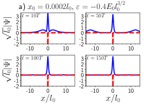
(a)

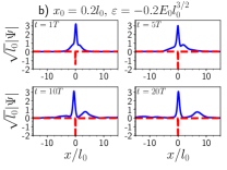
(b)

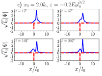
(c)

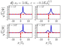
(d)

Figure 2: The same as in Fig. 1, but for the splitting of the breather under the action of the linear potential well, at values of $\varepsilon<0$, $x_{0}$, and $t$ indicated in panels.

As mentioned above, our goal is to investigate the fission of the breather into fragments, which will be mapped in the parameter plane of $\left(\varepsilon,x_{0}\right)$, for both $\varepsilon>0$ and $\varepsilon<0$, i.e., in the cases of the delta-like potential barrier and well. We find a certain threshold value of $x_{0}^{\mathrm{(crit)}}(\varepsilon>0)$ such that, at $|x|>x_{0}^{\mathrm{(crit)}}$ the breather does not split but bounces back as a whole from the potential barrier. In the next Section we demonstrate an analytical estimate for $x_{0}^{\mathrm{(crit)}}$, and then produce its numerically found values. Note that $x_{0}=0$ is a special situation that leads to a spontaneous symmetry breaking problem, in the form of spontaneous selection of the directions in which the two major fragments, which are close to solitons (6), move after completion of the fission. In numerical calculations, the symmetry-broken outcome may be determined by a weak random perturbation, if it is added to the input, simulating the real physical noise, either environmental or quantum. Numerical noise, induced by truncation error, leads to the symmetry breaking too, although its characteristics may differ from those of the physical noise. In this work we demonstrate that even a tiny shift of the input, such as $|x_{0}|=0.0002$, leads to the apparent symmetry breaking and fission of the breather, although the fission initiated by very small $|x_{0}|$ develops slowly, see Figs. 1a) and 1b).

The nonlinear barrier. It is also possible to consider the nonlinear potential barrier, based on equation

$$i\frac{\partial\Psi}{\partial t}=-\frac{1}{2}\frac{\partial^{2}\Psi}{\partial x^{2}}-\left[1-\frac{\varepsilon_{1}}{\sqrt{\pi}a}f(t)\exp\left(-\frac{x^{2}}{a^{2}}\right)\right]|\Psi|^{2}\Psi,$$ (10)

where $\varepsilon_{1}$ is the strength of the nonlinear potential. A permanent localized nonlinear potential was considered in Ref. HS , for splitting of an incident fundamental soliton, but not of a breather. The experimental realization of the nonlinear barrier in an atomic BEC was proposed in Ref. HS , assuming that a narrow laser beam is applied in a narrow region, reversing the local interaction between atoms from attractive to strongly repulsive.

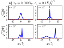
(a)

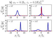
(b)

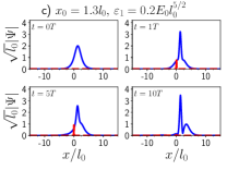
(c)

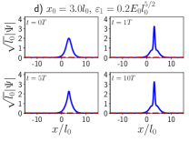
(d)

Figure 3: The same as in Fig. 1, but for the nonlinear splitter, defined as per Eq. (10). In this case, the red dashed line shows the shape of the splitting barrier, which includes factor $\left|\psi\left(x=0\right)\right|^{2}$, therefore the barrier disappears after the separation of the fragments.

III Numerical methods and analytical estimates

The evolution of the breather under the action of the splitting potential was simulated in the framework of Eq. (1) with $g=1$, using input (9), in which the remaining scaling invariance makes it possible to fix $A\equiv 1$, while keeping $\varepsilon$ and $x_{0}$ as free parameters. The simulations were carried out by means of the pseudospectral method to evaluate spatial derivatives, in a combination with the Runge-Kutta time-stepping scheme, to secure high accuracy of the results Y .

Proceeding to analytical estimates, one can evaluate the threshold value of the initial displacement, $x_{0}^{\mathrm{(crit)}}$, that separates the regimes of the bidirectional motion of fragments and unidirectional motion of the breather as a whole. In the case of large positive $\varepsilon$ and $\tau=0$ in Eqs. (1) and (3), one may assume, in the simplest approximation, that the input is cut by the tall barrier in two noncommunicating parts. In particular, the input located at $x<0$ may be defined as

$$\psi_{0}(x)=\left\{\begin{array}[]{c}2A~{}\mathrm{sech}\left[A\left(x-x_{0}\right)\right],~{}~{}\mathrm{at}~{}~{}x<0,\\ 0,~{}\mathrm{at}~{}~{}x>0.\end{array}\right.~{}$$ (11)

To estimate whether input (11) may or may not produce a soliton escaping to the left, it is possible to use the necessary condition for the generation of at least one NLS soliton in free space by a given input zakharov1984 :

$$\int_{-\infty}^{+\infty}\left|\psi_{0}(x)\right|dx>\ln\left(2+\sqrt{3}\right)\approx 1.32.$$ (12)

Roughly speaking, Eq. (12) may be understood as a threshold condition for the linear scattering problem associated with the NLS equation, i.e. the Zakharov-Shabat equations zakharov1972 , to have a bound state in the respective potential well. This is a difference from the linear Schrödinger equation, in which, as it is commonly known, an arbitrarily shallow potential well always maintains at least one bound state. If input (11) does not satisfy condition (12), it cannot generate a left-running soliton. Substituting expression (11) in Eq. (12) predicts a rough estimate for the threshold value $x_{0}^{\mathrm{(crit)}}$ which is a boundary for the generation of the left-traveling soliton:

$$A~{}x_{0}^{\mathrm{(crit)}}=\ln\left(\frac{4}{\ln\left(2+\sqrt{3}\right)}\right)\approx 1.11.$$ (13)

Additional analytical results may be produced by the conservation of the Hamiltonian (energy) corresponding to Eq. (1) (with $g=1$) at $t>\tau$, i.e., with $f=1$:

$$E=\frac{1}{2}\int_{-\infty}^{+\infty}\left(\left|\frac{\partial\psi}{\partial x}\right|^{2}-|\psi|^{4}\right)dx+\varepsilon\left|\psi\left(x=0\right)\right|^{2}.$$ (14)

The energy of the free-space fundamental solitons (6) contains the negative ground-state and positive kinetic terms, the effective mass of the soliton being $2A_{1,2}$ zakharov1984 :

$$\left(E_{\mathrm{sol}}\right)_{1,2}=-\frac{1}{3}A_{1,2}^{3}+A_{1,2}c_{1,2}^{2}~{}.$$ (15)

Note that, in the case of $\varepsilon=0$, the energy of the breather [the expectation value (14) for the solution (4)],

$$E_{\mathrm{br}}=-(28/3)A^{3},$$ (16)

is exactly equal to the sum of energies (15) with amplitudes taken as per Eq. (5), and $c_{1,2}=0$. In other words, this simple result corroborates the known fact that the binding energy of the breather, considered as a composite state of the constituent solitons, is exactly zero, in the framework of the integrable NLS equation. For given norm, the ground state of any physical setting modeled by the NLS equation is the fundamental soliton. In this connection, it is relevant to stress that the breather is not a ground state, but rather an excited one. Indeed, using Eqs. (15) and (16), it is easy to check that the energies of both states with equal norms are negative, with ratio $E_{\mathrm{sol}}/E_{\mathrm{br}}=16/7$.

Assuming that the breather has split in two fundamental solitons with these amplitudes and velocities $c_{1,2}\neq 0$, the energy conservation, taking into regard the term $\sim\varepsilon>0$ in Eq. (14) and neglecting a radiative component which may also appear in the output, yields the following constraint for the velocities:

$$3c_{1}^{2}+c_{2}^{2}=4\varepsilon A\mathrm{sech}^{2}\left(Ax_{0}\right).$$ (17)

Furthermore, in the case of $x_{0}=0$, the symmetry of the input conserves the total momentum (otherwise, the splitting potential breaks the conservation), which implies that the velocities of the fragments are related by constraint $3c_{1}+c_{2}=0$. In this case, Eq. (17) predicts the individual velocities:

$$c_{1}=-c_{2}/3=\pm\sqrt{\varepsilon A/3},$$ (18)

where $\pm$ implies that the spontaneous symmetry breaking may randomly send the soliton with velocity $c_{1}$ in either direction.

If a sufficiently strong perturbation transforms the initial breather (9) into a pair of fundamental solitons with the conservation of the total norm, i.e., $A_{1}+A_{2}=4A$, but the amplitude ratio $A_{1}:A_{2}$ different from $3:1$ [see, e.g., Fig. 3(a)], the comparison of energies (15) and (16) demonstrates that the energy of the soliton pair with zero velocities is larger than the initial energy in the case of $1<A_{1}:A_{2}<3$ (hence, this conversion scenario is suppressed), and is smaller in the cases of

$$A_{1}:A_{2}<1~{}~{}\mathrm{or~{}~{}}A_{1}:A_{2}>3,~{}$$ (19)

facilitating these scenarios.

In the model with a nonlinear splitting potential, which corresponds to Eq. (10), similar analytical predictions are produced by replacement $\varepsilon\rightarrow 2A^{2}\varepsilon_{1}$, i.e.,

$$3c_{1}^{2}+c_{2}^{2}=8\varepsilon_{1}A^{3}~{}\mathrm{sech}^{2}\left(Ax_{0}\right),$$ (20)

$$c_{1}=-c_{2}/3=\pm\sqrt{2\varepsilon_{1}A^{3}/3}~{}.$$ (21)

IV Results

The evolution of the breather interacting with the local potential is reported in Figs. 1, 2, and 3 by showing snapshots of numerically generated solutions to Eqs. (1) and (10), taken at different times. Further, the results are summarized below in Fig. 6 and, additionally, in Appendix (Figs. 9-17) by means of color-coded plots, which display amplitudes and velocities of the fragments, in the plane of $\left(\varepsilon,x_{0}\right)$ or $\left(\varepsilon_{1},x_{0}\right)$, for the linear and nonlinear splitting potentials, respectively.

IV.1 The linear potential barrier or well

In this subsection we present results obtained by solving Eq. 1 with the linear potential, defined according to Eqs. (2) and (3), and the input taken as per Eq. (4). The simulations reveal two main patterns of behavior: (i) the breather splits in two pulses close to fundamental solitons with the amplitude ratio close to $3:1$, cf. Eq. (6), moving in opposite directions; or (ii) the breather is pushed by the barrier to one side, again splitting in two solitons, subject to the same approximate amplitude ratio, $3:1$, but moving in one direction. Figure 1 displays snapshots of the simulations for different values of $x_{0}$ and $\varepsilon$, which illustrate these dynamical scenarios.

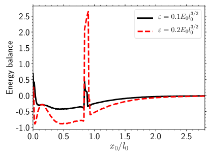
Figure 4: The difference of the left- and right-hand sides of Eq.  (17), as obtained from numerical data, illustrating the accuracy of the analytically predicted energy balance, for two values of the linear-barrier’s height, $\varepsilon=0.1$ and $0.2$.

In Fig. 4 we show values of $3c_{1}^{2}+c_{2}^{2}-4\varepsilon A^{2}\mathrm{sech}^{2}(Ax_{0})$ for $\varepsilon=0.1$ and $0.2$, to demonstrate accuracy of the analytical energy-balance constraint, predicted by Eq. (17), in comparison with the numerical results. Velocities of the fragments are evaluated numerically as

$$c_{j}=\frac{x_{j}(t_{\max})-x_{j}(t_{\max}/2)}{t_{\max}/2},$$ (22)

where $x_{j},~{}j=1,2$, are positions of the $j$-th peak, taken at times $t_{\max}=15T$ and $t_{\max}/2=7.5T$, to ensure that the peaks have separated (in most cases). It is seen that the predicted energy balance condition holds well for the two fragments that move in the same direction, but is completely broken in a vicinity of the critical point $x_{0}^{(\mathrm{crit})}$, as expected. For the two fragments moving in opposite directions, the energy balance is not satisfied very accurately, but the discrepancy is relatively small. Close to to the symmetry-breaking point, $x_{0}=0$, Fig. (4) shows that the analytically predicted condition is not satisfied either, due to the slow separation of the fragments, which means that the ballistic regime for the fragments was not yet achieved.

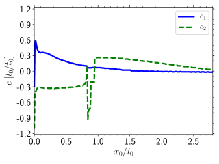
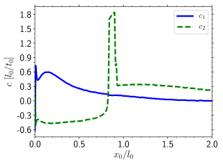
Figure 5: Velocities of the fragments, numerically identified according to Eq.  (22), as functions of $x_{0}$ for fixed values of the linear-barrier’s height, $\varepsilon=0.1$ and $\varepsilon=0.2$. The velocity of the heavier and lighter fragments, $c_{1}$ and $c_{2}$, are shown by the blue solid and green dashed curves, respectively

In Figs. 5 we show the velocities of the fragments according to the definition in Eq. (22) as functions of $x_{0}$ for fixed values of the barrier height, $\varepsilon=0.1$ and $\varepsilon=0.2$.

As mentioned above, point $x_{0}=0$ is a special one. Indeed, due to the symmetry of input Eq. (9), the breather cannot deterministically split into the solitons with unequal amplitudes. However, the symmetry may be spontaneously broken by an external perturbation. In Figs 1a) and 1b) we show that even a tiny change of the initial conditions leads to the symmetry breaking and, eventually, fission of the breather.

Typical examples of the interaction of the breather with the potential well ($\varepsilon<0$), displayed in Fig. 2, demonstrate that the breather does not split in the limit of small initial displacements, $x_{0}\rightarrow 0$. In this case [panel a) in the figure], the breather sheds off some radiation, and transforms into a fundamental soliton pinned to the potential well. When $x_{0}$ increases, the breather splits, but the fragments, being pulled by the attractive potential, separate much slower than in the case of the repulsive barrier, cf. Fig. 1. In particular, the heavier soliton may stay trapped by the potential well (performing small oscillations in this state), while the lighter one moves very slowly, as seen in panel b). This outcome of the interaction can be easily explained by the energy balance. Indeed, for small $|\varepsilon|$ comparison of the initial interaction energy, given by the last term in Eq. (14), with $\left|\psi\left(x=0\right)\right|^{2}=4A^{2}\mathrm{sech}^{2}\left(Ax_{0}\right)$, and a similar expression for the fundamental solitons with amplitudes Eq. (5), i.e., $\left|\psi\left(x=0\right)\right|^{2}=A_{1,2}^{2}$, demonstrates that the trapped state is energetically possible for the soliton with the larger amplitude, $A_{1}=3A$, in which case the energy-balance equation yields

$$c_{2}^{2}=|\varepsilon|A\left[9-4\mathrm{sech}^{2}\left(Ax_{0}\right)\right],$$ (23)

cf. Eqs. (17) and (18).

There are several possible regimes of the breather’s evolution following the interaction with the external potential: i) the initial breather splits in two soliton-like pulses that move bidirectionally; ii) the breather splits in two pulses that move unidirectionally; iii) the breather does not split clearly enough to distinguish the soliton-like fragments after the evolution time of the simulation; iv) the breather is transformed into a soliton bound by the trapping well; v) the breather does not split. In Fig. 6 we map these regimes in the parameters plane of $\left(\varepsilon,x_{0}\right)$. They are color-coded and denoted with Roman numerals. To plot the map in Fig. 6 we ran the simulations up to $t=15T$, and used the breather’s width, $l_{\mathrm{br}}=1/A$ , as a measure of the separation of the fragments. Thus, we categorize the breather as a split state when the distance between center-of-mass of the fragments is equal to or exceeds $l_{\mathrm{br}}$.

In Appendix we present the results for amplitudes and velocities of the two largest peaks in solution density at $t=15T$, in the form of color-coded maps in the plane of $\left(\varepsilon,x_{0}\right)$.

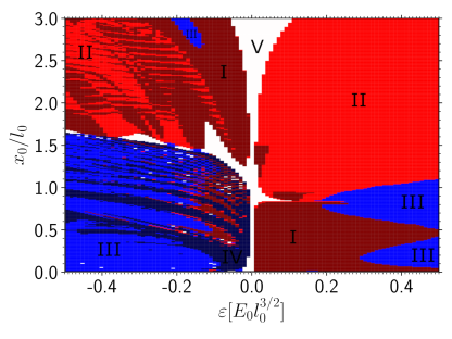
Figure 6: The linear splitter. The map of the regimes the splitting of the original breather in simulations of Eq. (1) at $t=15T$, in the plane of parameters $\varepsilon$ and $x_{0}$. Different regimes are color-coded and denoted by Roman numerals: I) the breather splits in two soliton-like fragments moving in opposite directions(brown); II) the breather splits in two soliton-like fragments moving in the same direction (red); III) the breather does not split clearly enough in the course of the simulation time, $t=15T$ (blue); IV) the breather splits in a heavies soliton-like fragment, bound by the attractive potential, and radiation (dark blue); V) the breather does not split (white).

IV.2 The nonlinear potential barrier

In the case of the nonlinear potential defined by Eq. (10), the difference from its linear-potential counterpart is that, as the strength of the nonlinear barrier depends on the local density at $x=0$, the action of the effective potential subsides in the course of splitting. Typical examples of the interaction of the breather with the nonlinear splitter are presented in Fig. 3. As in the case of the linear barrier, even a tiny asymmetry in the initial conditions, with $|x_{0}|=0.0002$, breaks the symmetry of the problem and leads to fission of the breather. The resulting amplitude ratio is $\simeq 10:1$, which is much larger than the “natural” one, $3:1$. In Fig. 7 we show the accuracy of the energy balance for the nonlinear barrier, as predicted by Eq. (20). We see that, similarly to the linear barrier, the predicted condition is very accurate for the fragments moving in the same direction, and is broken in a vicinity of the critical point $x_{0}^{(\mathrm{crit})}$, as expected. However, the breaking of the predicted energy-balance condition is much more pronounced in the case of the nonlinear potential, as seen in the $x_{0}<x_{0}^{(\mathrm{crit})}$ segment of Fig. 7.

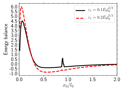
Figure 7: The same as in Fig. 4, but for the energy balance predicted by Eq. (20) for two values of the nonlinear barrier height, $\varepsilon=0.1$ and $0.2$.

In Figs. 8 we plot the velocities of the two largest density peaks following the interaction of the input with the nonlinear barrier, that are identified as per Eq. (22).

Just as for the linear splitting potential, there are several possible regimes of the breather’s evolution after the interaction with the nonlinear splitter: i) the initial breather splits into two soliton-like pulses that move bidirectionally; ii) the breather does not split clearly enough to distinguish soliton-like fragments after the simulation time; iii) the breather splits in two soliton-like unidirectionally moving pulses; iv) the breather splits in a soliton and radiation; v) the breather does not split. In Fig. 9 we map these regimes in the parameters plane of $\left(\varepsilon,x_{0}\right)$. The different regimes are color-coded and denoted by Roman numerals. For the map in Fig. 9 we ran the simulations up to $t=15T$, and used the width of a breather, $l_{\mathrm{br}}=1/A$ , as a measure of the separation of the fragments.

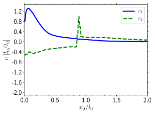
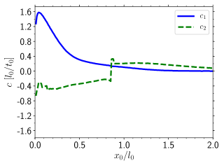
Figure 8: Velocities of the fragments, identified as per Eq. (22), as functions of $x_{0}$ for fixed values of the nonlinear-barrier’s height, $\varepsilon_{1}=0.1$ and $\varepsilon=0.2$. The velocities of the heavier and lighter fragment, $c_{1}$ and $c_{2}$, are shown by the blue solid and green dashed curves, respectively.

We see that in the case of the nonlinear potential the general character of the breather’s splitting is similar to the case of the linear repulsive barrier. However, the region where both fragments travel in the same direction is much smaller, in comparison to the latter case.

The results for amplitudes and velocities of the two largest density peaks of the solution at $t=15T$, in the form of color-coded maps in the plane of $\left(\varepsilon,x_{0}\right)$, for the setting with the nonlinear barrier are displayed in Appendix too.

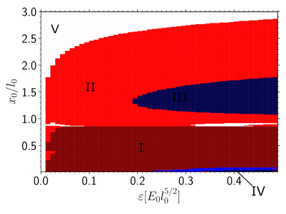
Figure 9: The nonlinear splitter. The map of splitting regimes for the original breather in simulations of Eq. (10) at $t=15T$, in the plane of parameters $\varepsilon_{1}$ and $x_{0}$. Different regimes are color-coded and denoted by Roman numerals: I) the breather splits in two soliton-like fragments moveing in opposite directions(brown); II) the breather is not separated clearly enough at $t=15T$ (red); III) the breather splits in two soliton-like fragments moving in the same direction (dark blue); IV) the breather splits in one soliton and radiation (blue); V) the breather does not split.

V Conclusion

The subject of the work is the dynamics of NLS breathers interacting with localized linear and nonlinear splitting potentials. The setting applies to matter-wave states in a BEC, as well as to optical beams and pulses, in the spatial and temporal domains, respectively. The potentials are approximated by the delta-function, and by its regularized version, as concerns the numerical scheme. The linear splitter may be represented by a narrow barrier or potential well (the nonlinear splitter is considered only with the repulsive sign). The potentials breaks the integrability of the NLS equation, leading to various dynamical scenarios. Depending on the initial position of the breather with respect to the localized splitting potential, it may split into a pair of fundamental solitons, moving in opposite directions, or bounce as a whole. In the former case, the amplitude ratio of the fragments may be both close to the expected value $3:1$, predicted by the exact solution for the NLS breather, and strongly different from it (especially in the case of the nonlinear splitter). When the center of the initial breather is very close to the position of the barrier’s center, the linear potential well leads to another outcome of the interaction, with the larger-amplitude soliton staying trapped by the attractive well, while the smaller-amplitude one slowly escapes. Post-splitting velocities of the solitons may be predicted by means of the analytical energy balance.

There are several avenues to explore as a follow-up to this work. First and foremost, one may consider splitting potentials with shapes that are closer to experimentally realistic ones. For getting closer to the experimentally relevant setting in BEC, it may also be necessary to consider the full three-dimensional model, rather than its one-dimensional reduction, cf. Ref. we . Another relevant extension may be inclusion of quantum noise, again in terms of a BEC. In particular, quantum fluctuations may govern the spontaneous symmetry breaking in the case of $x_{0}=0$.

VI Acknowledgement

This work is jointly supported by the National Science Foundation through grants No. PHY-1402249 and No. PHY-1607221 and the Binational (US-Israel) Science Foundation through grant No. 2015616,and by Israel Science Foundation (project No. 1287/17). The work at Rice was supported by the Army Research Office Multidisciplinary University Research Initiative (Grant No. W911NF-14-1-0003), the Office of Naval Research, the NSF (Grant No. PHY-1707992), and the Welch Foundation (Grant No. C-1133).

*

Appendix A Amplitude and velocity heatmaps

In this Appendix we present additional computational results, namely two-dimensional maps of the amplitudes and velocities of the heavier and lighter fragments in the settings with both linear and nonlinear localized potentials.

A.1 The linear splitter

Results for the heavier and lighter fragments are collected in Figs. 10 and 11, in the form of color-coded maps in the plane of $\left(\varepsilon,x_{0}\right)$, which also include the data produces for $\varepsilon<0$, i.e., for the splitting produced by the interaction of the breather with the narrow potential well. These figures, along with Fig. 1, clearly demonstrate that, in the majority of cases in the case of splitting barrier, $\varepsilon>0$, the amplitude ratio for the fragments remains close to the expected value $3:1$.

Results for velocities of the fragments are collected in Figs. 12 and 13. In particular, the former figure demonstrates that the sign of the velocity of the heavier soliton is always identical to the sign of $x_{0}$, whereas the it is seen in Fig. 13 that the lighter soliton moves in the opposite direction at

$$\left|x_{0}\right|<x_{0}^{\mathrm{(crit)}}\approx 0.9,$$ (24)

and changes the sign of its velocity at $\left|x_{0}\right|>x_{0}^{\mathrm{(crit)}}$, moving in the same direction as its heavier counterpart. Note that the value of $x_{0}^{\mathrm{(crit)}}$is rather close to the one predicted above by the crude analytical approximation, see Eq. (13). Lastly, the numerical results for the velocities approximately corroborate the analytical prediction produced by Eqs. (17) and (18).

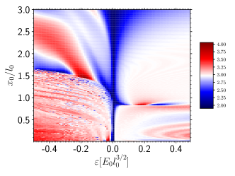
Figure 10: The linear splitter. The map of the amplitude of the heavier soliton produced by the splitting of the original breather in simulations of Eq. (1) at $t=15T$, in the plane of parameters $\varepsilon$ and $x_{0}$. Black dashed lines, separating different regions in the diagram, serve to highlight the difference between colors in the map.

The results for the potential well ($\varepsilon<0$) are summarized, along with their counterparts for the barrier ($\varepsilon>0$) in the amplitude- and velocity-distribution maps displayed in Figs. 10-13. The maps show that the regions for $\varepsilon<0$ feature more elaborate structure than $\varepsilon>0$, and, as mentioned above, much smaller velocities. In fact, a larger part of the velocity maps for $\varepsilon<0$ is accounted for by small oscillations of the trapped soliton with amplitude $A_{1}$.

The comparison of the analytical energy-balance prediction for the case of the potential well, given by Eq. (23), with the numerical results demonstrates that the analytical prediction overestimates velocity $c_{2}$. The discrepancy is explained by the fact that the radiation shed off by the splitting breather carries away a large portion of the energy, which is not taken into account by the analytical approximation.

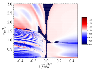
Figure 11: The linear splitter. The same as in Fig. 10, but for the amplitude of the lighter soliton produced by the splitting of the original breather.

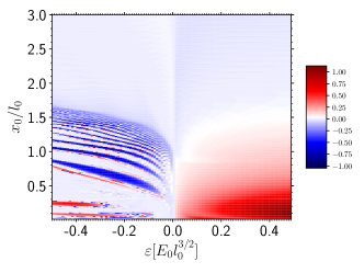
Figure 12: The linear splitter. The map of values of the velocity of the heavier soliton, produced by the splitting of the original breather in simulations of Eq. (1) at $t=15T$, in the plane of parameters $\varepsilon$ and $x_{0}$. Black dashed lines, separating different regions in the diagram, serve as a guide to the eye. The light blue hue for large values of $x_{0}$ corresponds to zero velocity.

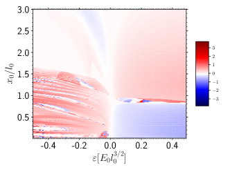
Figure 13: The linear splitter. The same as in Fig. 12, but for the velocity of the lighter soliton (the one with a smaller amplitude).

A.2 The nonlinear splitter

The results are summarized in the form of maps for amplitude and velocities distributions in the plane of $\left(\varepsilon_{1},x_{0}\right)$, which are displayed in Figs. 14-17. In comparison to the results reported above for the linear barrier, the boundary between splitting and non-splitting regimes (where the breather bounces from the barrier and thus avoids the splitting) is much sharper in the present case, although it remains close to approximately the same critical position, $x_{0}^{\mathrm{(crit)}}\approx 0.9$, see Eq. (24). Another difference is that the amplitude ratio of the fragments tends to deviate from the “natural” ratio $3:1$ (e.g., ratio $\simeq 10:1$ corresponding to $x_{0}=0$), and their velocities are much smaller than in the case of the linear splitter.

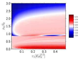
Figure 14: The nonlinear splitter. The map of the amplitude of the larger soliton produced by the splitting of the original breather in simulations of Eq. (10) at $t=15T$, in the plane of parameters $\varepsilon_{1}$ and $x_{0}$.

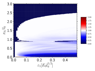
Figure 15: The nonlinear barrier. The same as in Fig. 14, but for the amplitude of the lighter soliton produced by the splitting of the original breather.

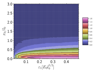
Figure 16: The nonlinear splitter. The map of values of the velocity of the heavier soliton, produced by the splitting of the original breather in simulations of Eq. (10) at $t=15T$, in the plane of parameters $\varepsilon_{1}$ and $x_{0}$.

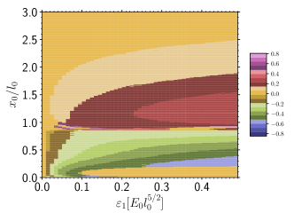
Figure 17: The nonlinear barrier. The same as in Fig. 16, but for the velocity of the lighter soliton (the one with the smaller amplitude).

References

- (1) Y. S. Kivshar and G. P. Agrawal, Optical Solitons: From Fibers to Photonic Crystals (Academic Press, San Diego, 2003).
- (2) T. Dauxois and M. Peyrard, Physics of Solitons (Cambridge University Press: Cambridge, UK, 2006).
- (3) J. Yang, Nonlinear Waves in Integrable and Nonintegrable Systems (SIAM: Philadelphia, 2010).
- (4) K. E. Strecker, G. B. Partridge, A. G. Truscott, and R. G. Hulet, Formation and propagation of matter-wave soliton trains, Nature, 417, 150-153 (2002).
- (5) L. Khaykovich, F. Schreck, G. Ferrari, T. Bourdel, J. Cubizolles, L. D. Carr, Y. Castin, and C. Salomon, Formation of a matter-wave bright soliton. Science, 296(5571), 129-1293 (2002).
- (6) K. E. Strecker, G. B. Partridge, A. G. Truscott, and R. G. Hulet, Bright matter wave solitons in Bose-Einstein condensates, New J. Phys. 5, 73 (2003).
- (7) S. L. Cornish, S. T. Thompson, and C. E. Wieman, Formation of bright matter-wave solitons during the collapse of attractive Bose-Einstein condensates, Phys. Rev. Lett. 96, 170401 (2006).
- (8) A. L. Marchant, T. P. Billam, T. P. Wiles, M. M. H. Yu, S. A. Gardiner, and S. L. Cornish, Controlled formation and reflection of a bright solitary matter-wave, Nature Commun. 4, 1865 (2013).
- (9) L. P. Pitaevskii and A. Stringari, Bose-Einstein Condensation (Clarendon Press: Oxford, 2003).
- (10) V. E. Zakharov and A. B. Shabat, Exact theory of two-dimensional self-focusing and one-dimensional self-modulation of waves in nonlinear media, J. Exp. Theor. Phys. 34, 1 62 (1972).
- (11) J. Satsuma and N. Yajima, Initial value problems of one-dimensional self-modulation of nonlinear waves in dispersive media. Suppl. Progr. Theor. Phys. 55, 284-306 (1974).
- (12) V. E. Zakharov, S. V. Manakov, S. P. Novikov, and L. P. Pitaevskii, Theory of Solitons (Nauka, Moscow, 1980); English translation: Consultants Bureau, New York, 1984.
- (13) E. H. Lieb and W. Liniger, Phys. Rev. 130, 1605 (1963).
- (14) V. A. Yurovsky, M. Olshanii, and D. S. Weiss, Adv. At. Mol. Opt. Phys. 55, 61 (2008).
- (15) V. A. Yurovsky, B. A. Malomed, R. G. Hulet, and M. Olshanii, Dissociation of one-dimensional matter-wave breathers due to quantum many-body effects, Phys. Rev. Lett. 119, 220401 (2017).
- (16) H. Sakaguchi and B. A. Malomed, Resonant nonlinearity management for nonlinear Schrödinger solitons, Phys. Rev. E 70, 066613 (2004).
- (17) H. Yanai, L. Khaykovich, and B. A. Malomed, Stabilization and destabilization of second-order solitons against perturbations in the nonlinear Schrödinger equation, Chaos 19, 033145 (2009).
- (18) V. Dunjko and M. Olshanii, Superheated integrability and multisoliton survival through scattering off barriers, arXiv:1501.00075.
- (19) B. A. Malomed, N. N. Rosanov, and S. V. Fedorov, Dynamics of nonlinear Schrödinger breathers in a potential trap. Physical Review E, 97, 052204 (2018).
- (20) J. Golde, J. Ruhl, B. A. Malomed, M. Olshanii, and V. Dunjko, Metastability versus collapse following a quench in attractive Bose-Einstein condensates, Phys. Rev. A 97, 053604 (2018).
- (21) Y. S. Kivshar and D. K. Campbell, Peierls-Nabarro potential barrier for highly localized nonlinear modes, Phys. Rev. E 48, 3077-3081 (1993).
- (22) V. Hakim, Nonlinear Schrödinger flow past an obstacle in one dimension, Phys. Rev. E 55, 2835-2845 (1997).
- (23) L. Salasnich, Pulsed quantum tunneling with matter waves, Laser Phys. 12, 198-202 (2002).
- (24) N. Moiseyev and L. S. Cederbaum, Resonance solutions of the nonlinear Schrödinger equation: Tunneling lifetime and fragmentation of trapped condensates, Phys. Rev. A 72, 033605 (2005).
- (25) T. L. Belyaeva, V. N. Serkin, C. Hernandez-Tenorio, and F. Garcia-Santibanez, Enigmas of optical and matter-wave soliton nonlinear tunneling, J. Mod. Opt. 57, 1087-1099 (2010).
- (26) J. L. Helm,T. P. Billam, and S. A. Gardiner, Bright matter-wave soliton collisions at narrow barriers, Phys. Rev. A 85, 053621 (2012).
- (27) F. Kh. Abdullaev and V. A. Brazhnyi, Solitons in dipolar Bose–Einstein condensates with a trap and barrier potential, J. Phys. B: At. Mol. Opt. Phys. 45, 085301 (2012).
- (28) J. L. Helm, T. P. Billam, and S. A. Gardiner, Bright matter-wave soliton collisions at narrow barriers, Phys. Rev. A 85, 053621 (2012).
- (29) J. Cuevas, P. G. Kevrekidis, B. A. Malomed, P. Dyke, and R. G. Hulet, Interactions of solitons with a Gaussian barrier: Splitting and recombination in quasi-1D and 3D, New J. Phys. 15, 063006 (2013).
- (30) P. Manju, K. S. Hardman, M. A. Sooriyabandara, P. B. Wigley, J. D. Close, N. P. Robins, M. R. Hush, and S. S. Szigeti, Quantum tunneling dynamics of an interacting Bose-Einstein condensate through a Gaussian barrier, Phys. Rev. A 98, 053629 (2018).
- (31) C. Lee and J. Brand, Enhanced quantum reflection of matter-wave solitons, Europhys. Lett. 73, 321-327 (2006).
- (32) T. Ernts and J. Brand, Resonant trapping in the transport of a matter-wave soliton through a quantum well, Phys. Rev. A 81, 033614 (2010).
- (33) N. Veretenov, Yu. Rozhdestvensky, N. Rosanov, V. Smirnov, and S. Fedorov, Interferometric precision measurements with Bose–Einstein condensate solitons formed by an optical lattice, Eur. Phys. J. D 42, 455-460 (2007).
- (34) B. Gertjerenken and C. Weiss, Nonlocal quantum superpositions of bright matter-wave solitons and dimers, J. Phys. B: At. Mol. Opt. Phys. 45, 165301 (2012),
- (35) Y. Kageyama and H. Sakaguchi, Reflection of channel-guided solitons at corners and junctions in two-dimensional nonlinear Schrödinger equation, J. Phys. Soc. Jpn. 81, 033001 (2012).
- (36) A. D. Martin and J. Ruostekoski, Quantum dynamics of atomic bright solitons under splitting and recollision, and implications for interferometry, New J. Phys. 14, 043040 (2012).
- (37) J. Polo and V. Ahufinger, Soliton-based matter-wave interferometer, Phys. Rev. A 88, 053628 (2013).
- (38) J. L. Helm, S. J. Rooney, C. Weiss, and S. A. Gardiner, Splitting bright matter-wave solitons on narrow potential barriers: Quantum to classical transition and applications to interferometry, Phys. Rev. A 89, 033610 (2014).
- (39) J. L. Helm, S. J. Rooney, C. Weiss, and S. A. Gardiner, Splitting bright matter-wave solitons on narrow potential barriers: Quantum to classical transition and applications to interferometry, Phys. Rev. Lett. 114, 134101 (2015).
- (40) G. D. McDonald, C. C. N. Kuhn, K. S. Hardman, S. Bennetts, P. J. Everitt, P. A. Altin, J. E. Debs, J. D. Close, and N. P. Robins, Bright solitonic matter-wave interferometer, Phys. Rev. Lett. 113, 013002 (2014).
- (41) P. Dyke, L. Sidong, S. Pollack, D. Dries, and R. Hulet, Interactions of bright matter-wave solitons with a barrier potential, In 42nd Annual Meeting of the APS Division of Atomic, Molecular and Optical Physics 56, OPE. 10 (2011).
- (42) H. Sakaguchi and B. A. Malomed, Matter-wave soliton interferometer based on a nonlinear splitter, New J. Phys. 18, 025020 (2016).
- (43) A. Shipulin, G. Onishchukov, and B. A. Malomed, Suppression of the soliton jitter by a copropagating support structure, J. Opt. Soc. Am. B 14, 3393-3402 (1997).
- (44) M. Olshanii, Atomic scattering in the presence of an external confinement and a gas of impenetrable bosons. Phys. Rev. Lett. 81, 938-941 (1998).
*