Random walks in non-Poissoinan activity driven temporal networks

Abstract

The interest in non-Markovian dynamics within the complex systems community has recently blossomed, due to a new wealth of time-resolved data pointing out the bursty dynamics of many natural and human interactions, manifested in an inter-event time between consecutive interactions showing a heavy-tailed distribution. In particular, empirical data has shown that the bursty dynamics of temporal networks can have deep consequences on the behavior of the dynamical processes running on top of them. Here, we study the case of random walks, as a paradigm of diffusive processes, unfolding on temporal networks generated by a non-Poissonian activity driven dynamics. We derive analytic expressions for the steady state occupation probability and first passage time distribution in the infinite network size and strong aging limits, showing that the random walk dynamics on non-Markovian networks are fundamentally different from what is observed in Markovian networks. We found a particularly surprising behavior in the limit of diverging average inter-event time, in which the random walker feels the network as homogeneous, even though the activation probability of nodes is heterogeneously distributed. Our results are supported by extensive numerical simulations. We anticipate that our findings may be of interest among the researchers studying non-Markovian dynamics of time-evolving complex topologies.

I Introduction

Temporal networks Holme (2015); Lambiotte and Masuda (2016) constitute a recent new description of complex systems, that, moving apart for the classical static paradigm of network science Newman (2010), in which nodes and edges do not change in time, consider dynamic connections that can be created, destroyed or rewired at different time scales. Within this framework, a first round of studies proposed temporal network models ruled by homogeneous Markovian dynamics Gauvin et al. (2018). A prominent example is represented by the activity-driven model Perra et al. (2012a), in which nodes are characterized by a different degree of activity, i.e. the constant rate at which an agent sends links to other peers, following a Poissonian process. The memoryless property implied by the Markovian dynamics greatly simplifies the mathematical treatment of these models, regarding both the topological properties of the time-integrated network representation Starnini and Pastor-Satorras (2013), and the description of the dynamical processes unfolding on activity-driven networks Perra et al. (2012b); Starnini and Pastor-Satorras (2014); Liu et al. (2014); Alessandretti et al. (2017); Pozzana et al. (2017); Nadini et al. (2018).

However, the Markovian assumption in temporal network modeling has been challenged by the increasing availability of time-resolved data on different kinds of interactions, ranging from phone communications Onnela et al. (2007) and face-to-face interactions Cattuto et al. (2010), to natural phenomena Corral (2004); Wheatland et al. (1998) and biological processes Kemuriyama et al. (2010). These empirical observations have uncovered a rich variety of dynamical properties, in particular that the inter-event times $t$ between two successive interactions (either the creation of the same edge or two consecutive creations of an edge by the same node), $\psi(t)$, follows heavy-tailed distributions Barabàsi (2005); Cattuto et al. (2010); Holme (2003). This bursty dynamics Barabàsi (2005) is a clear signature that the homogeneous temporal process description is inadequate and that non-Markovian dynamics lie at the core of such interactions. As a consequence, the interest in non-Markovian dynamics within the complex systems community has recently blossomed, from the point of view of both mathematical modeling Moinet et al. (2015); Karsai et al. (2014); Vestergaard et al. (2014); García-Pérez et al. (2015); Jo et al. (2014); Kiss et al. (2015); Scholtes et al. (2014) and dynamical processes, especially regarding epidemic spreading Van Mieghem and van de Bovenkamp (2013); Starnini et al. (2017); Boguñá et al. (2014); Sun et al. (2015). Within the framework of non-Markovian networks modeling, the Non-Poissoinan activity driven (NoPAD) model Moinet et al. (2015, 2016) offers a simple, mathematically tractable framework aimed at reproducing empirically observed inter-event time distributions, overcoming the limitations of the classical activity-driven paradigm.

The bursty nature of temporal networks can have a deep impact on dynamical processes running on top of them, ranging form epidemic spreading, percolation, social dynamics or synchronization; see Ref. Porter and Gleeson (2016) for a bibliographical summary. Among the many dynamical processes studied on temporal networks, the random walk stands as one of the most considered, due to its simplicity and wide range of practical applications Weiss (1994); Masuda et al. (2017). Traditional approaches are based on the concept of continuous time random walks Klafter and Sokolov (2011), where the random walk is represented as a renewal process Cox (1967), in which the probability per unit time that the walker exits a given node through an edge is constant. This Poissonian approximation Klafter and Sokolov (2011), which translates in a waiting time of the walker inside each node with an exponential distribution, permits an analytic approach based on a generalized master equation Weiss (1994). The Poissonian case has been considered in particular for activity-driven networks Perra et al. (2012b); Alessandretti et al. (2017); Sousa da Mata and Pastor-Satorras (2015).

However, if the inter-event time distribution $\psi(t)$ is not exponential, as empirically observed, the waiting time of the random walker shows aging effects, meaning that the time at which the walker will leave one node depends on the exact time at which it arrived at the considered node. Such memory effects are particularly important when the inter-event time distribution lacks a first moment Schulz et al. (2014). A way to neglect these aging effects is by considering active random walks, in which the inter-event time of a node is reinitialized when a walker lands on it, in such a way that intervent and waiting time distributions coincide. In opposition, in passive random walks the presence of the walker does not reinitialize the inter-event times of nodes or edges, and thus the waiting time depends on the last activation time Speidel et al. (2015). The non-Poissoinan scenario has been considered in the general context of a fixed network in which edges are established according to a given inter-event time distribution $\psi_{ij}(t)$ for active walkers Hoffmann et al. (2012); Speidel et al. (2015); de Nigris et al. (2016) and for passive walkers Speidel et al. (2015), usually with the assumption of a finite average inter-event time distribution, with the exception of Ref. de Nigris et al. (2016).

In this paper, we contribute to this endeavor with the study of passive random walks on temporal networks characterized by non-Markovian dynamics, by considering the case of networks generated by the NoPAD model. In the NoPAD model, nodes establish connections to randomly chosen neighbors following a heavy-tailed inter-event time distribution $\psi_{c}(t)\sim t^{-1-\alpha}$, with $0<\alpha<2$, depending on an activity parameter $c$ assigned to each node Moinet et al. (2015, 2016). We show that the dynamics of passive random walks on NoPAD networks fundamentally departs from the one observed on classical Poissonian activity-driven networks. For the case $\alpha>1$, when the average inter-event time is finite, we observe that the passive random walk behaves in the infinite network limit as an active one with inter-event time distribution $\psi_{c}(t)\sim t^{-\alpha}$. For the more interesting case $\alpha<1$, we argue that a passive random walk behaves, in the large time limit, as a walker in a homogeneous network. Our results are checked against extensive numerical simulations.

The paper is organized as it follows: In Section II we present the definition of passive random walks on NoPAD networks. Sect. III presents a general formalism for the walker occupation probability and first passage time distribution, that can be further elaborated in Laplace space in the case $\alpha>1$, corresponding to an inter-event time distribution with finite first moment. We present the application of this formalism for the standard Poissonian activity driven model in Sec. IV, recovering previously known results. In Sec. V we consider NoPAD networks with finite average inter-event times. The case of infinite average inter-event times is discussed in Sec. VI. Our conclusions are finally presented in Sec. VII.

II Passive random walks on NoPAD networks

In the NoPAD model  Moinet et al. (2015, 2016), nodes establish instantaneous connections with randomly chosen peers by following a renewal process. Each node is activated independently from the others, with the same functional form of the inter-event time distribution $\psi_{c}(t)\sim t^{-\alpha-1}$, with $\alpha>0$, between consecutive activation events, which depends on an activity parameter $c$, heterogeneously distributed among the population with a probability distribution $\eta(c)$. The dynamics of a random walk on NoPAD networks is defined as follows: A walker arriving at a node $i$ at time $t$ remains on it until an edge is created joining $i$ and another randomly chosen node $j$ at a subsequent time $t^{\prime}>t$, after a waiting time $t^{\prime}-t$ has elapsed. The walker then jumps instantaneously to node $j$ and waits there until an edge departing from $j$ is created at a subsequent time $t^{\prime\prime}>t^{\prime}$. To simplify calculations, here we will focus on directed random walks: a walker can leave node $i$ only when $i$ becomes active and creates an edge pointing to another node Perra et al. (2012b); Sousa da Mata and Pastor-Satorras (2015). We consider the case of a passive random walk: the internal clock of the host node $i$ is not affected by the walker’s arrival, and it must wait there until $i$ creates a new connection. With this definition, a directed random walk on a NoPAD network can be mapped to a continuous time random walk on a fully connected network in which each node has a different distribution of waiting times. We assume that all nodes are synchronized at a time $-t_{a}<0$ (i.e., the internal clock of all nodes is set to zero at time $-t_{a}$ or, in other words, we assume the all nodes become active at time $-t_{a}$) and that the random walk starts at time $t=0$ from a node with activity $c$, chosen for generality with probability distribution $H(c)$.

For a general inter-event time distribution $\psi_{c}(t)$, it is important to recall that the relevant quantity to describe the motion of a random walker is the waiting time distribution of residence inside each node. If $\psi_{c}(t)$ takes an exponential form, the activation rate is constant, implying that the time to the next activation is independent of the time of the last one. In this case, the waiting time distribution coincides with $\psi_{c}(t)$ and memory effects are absent Cox (1967). When $\psi_{c}(t)$ has a non-exponential form, the waiting time distribution is different from $\psi_{c}(t)$ and indeed it takes a non-local form: A walker arriving at a node with activity $c$ at time $t$, it will jump out of it at the next activation event of this node. Assuming the previous activation event took place at time $t_{p}<t$, the next one will take place at time $t_{n}$, where the inter-event time $\Delta t=t_{n}-t_{p}$ is randomly distributed according to $\psi_{c}(\Delta t)$. The waiting time of the walker in node with activity $c$ is thus given by $\tau=t_{n}-t$ and depends explicitly on the immediately previous activation time $t_{p}$. An exact description of the passive walker will thus require knowledge of the complete trajectory of the walker in the network, and of the whole sequence of activation times of all nodes Speidel et al. (2015).

This requirement can be however relaxed in the case of NoPAD networks. In the class of activity driven networks, after an activation event, the walker jumps to a randomly chosen node. Thus, in the limit of an infinite network, each node traversed in the path of the walker is essentially visited for the first time. Therefore, the random walker waiting time distribution depends not on the whole walker path, but only on the temporal distance to the synchronization point. In these terms, we consider as the waiting time distribution the forward inter-event time distribution Klafter and Sokolov (2011), $h_{c}(t_{a}+t^{\prime},t)$, defined as the probability that a walker arriving on a node with activity $c$ at time $t^{\prime}$ (hence at a time $t_{a}+t^{\prime}$ measured from the synchronization point of all nodes in the network) will escape from it, due to the activation of the node, at a time $t^{\prime}+t$, or, in other words, that it will wait at the node for a time interval $t$. When the inter-event time distribution is exponential, corresponding to a memory-less Poisson process, one has $h_{c}(t_{a}+t^{\prime},t)\equiv\psi_{c}(t)$, independent of both the aging time $t_{a}$ and the arrival time $t^{\prime}$ of the walker Cox (1967). For general forms of the inter-event time distribution $\psi_{c}(t)$, aging effects take place and the function $h_{c}$ depends explicitly on the arrival time $t^{\prime}$ Schulz et al. (2014).

III General formalism

In this Section we develop a general formalism to compute the steady state occupation probability and the first passage time properties of the passive random walk in infinite NoPAD networks. In the case of an inter-event time distribution with finite first moment, and in the limit of an infinitely aged network ($t_{a}\to\infty$) we can pass to Laplace space to provide closed-form expressions.

III.1 Occupation probability

We consider here the occupation probability $P(c,t|c_{0})$, defined as the probability that a walker is at a node with activity $c$ at time $t$, provided it started at time $t=0$ on a node with activity $c_{0}$. To compute it, let us define the probability $\Phi_{n}(c,t|c_{0})$ that a walker starting at $c_{0}$ has performed $n$ hops at time $t$, landing at the last hop, made at time $t^{\prime\prime}$, with $0<t^{\prime\prime}<t$, at a node with activity $c$. These two probabilities are trivially related by the expression

$$P(c,t|c_{0})=\sum_{n=0}^{\infty}\Phi_{n}(c,t|c_{0}).$$ (1)

For $n=0$ (the node $c_{0}$ does not become activated during the whole time $t$), we have

$$\Phi_{0}(c,t|c_{0})=\tilde{h}_{c_{0}}(t_{a},t)\delta_{c,c_{0}},$$ (2)

where $\delta_{c,c^{\prime}}$ is the Kronecker symbol and we have defined

$$\tilde{h}_{c}(t_{a}+t^{\prime},t)=\int_{t}^{\infty}h_{c}(t_{a}+t^{\prime},\tau)\,d\tau$$ (3)

as the probability that a walker arriving at time $t^{\prime}$ on a node $c$ has not left it up to time $t+t^{\prime}$.

To calculate $\Phi_{n}(c,t|c_{0})$ for $n\geq 1$ we make use of a self-consistent condition. Defining $\Psi_{n}(t|c_{0})$ as the probability that the $n$-th jump of a walker starting at $c_{0}$ takes place exactly at time $t$, we can write

$$\Phi_{n}(c,t|c_{0})=\int_{0}^{t}\Psi_{n}(t^{\prime}|c_{0})\eta(c)\tilde{h}_{c}(t_{a}+t^{\prime},t-t^{\prime})\,dt^{\prime}.$$ (4)

This equation expresses the sum of the probabilities of the events in which the walker performs its $n$-th jump at any time $t^{\prime}<t$, arrives in this jump at a node $c$, given by the probability $\eta(c)$, and rests at that node $c$ for a time larger than $t-t^{\prime}$. To compute $\Psi_{n}(t|c_{0})$ we apply another self-consistent condition, namely

$$\Psi_{n}(t|c_{0})=\sum_{c^{\prime}}\int_{0}^{t}\Psi_{n-1}(t^{\prime}|c_{0})\eta(c^{\prime})h_{c^{\prime}}(t_{a}+t^{\prime},t-t^{\prime})\,dt^{\prime}.$$ (5)

This equation implies the $(n-1)$-th jump taking place at time $t^{\prime}$, and landing on a node $c^{\prime}$, with probability $\eta(c^{\prime})$, and the last jump taking place, from $c^{\prime}$, at time $t-t^{\prime}$. The expression is averaged over all possible values of the activity $c^{\prime}$ of the intermediate step. The iterative Eq. (5), complemented with the initial condition $\Psi_{1}(t|c_{0})=\tilde{h}_{c_{0}}(t_{a},t)$, provides a complete solution for the steady state probability, via Eqs. (4) and (1).

III.2 First passage time distribution

We now consider the first passage time probability $F(t,c|c_{0})$, defined as the probability that a walker starting at a node of activity $c_{0}$ arrives for the first time at another node of activity $c$ exactly at time $t$. To compute it, we define $\bar{\Psi}_{n}(t|c,c_{0})$ as the probability that the walker performs his $n$-th hop at time $t$, irrespective of where it lands, in a trajectory that has never visited before a node of activity $c$. We can thus write

$$F(t,c|c_{0})=h_{c_{0}}(t_{a},t)\eta(c)+\int_{0}^{t}dt^{\prime}\sum_{n=1}^{\infty}\bar{\Psi}_{n}(t^{\prime}|c,c_{0})\sum_{c^{\prime}\neq c}\eta(c^{\prime})h_{c^{\prime}}(t_{a}+t^{\prime},t-t^{\prime})\eta(c).$$ (6)

In this equation, the first term accounts for the walker arriving at $c$ in a single hop, while for the second term we consider that the walker has performed an arbitrary number of hops $n\geq 1$ at a time $t^{\prime}$, that the last of these hops lands on a node with activity $c^{\prime}\neq c$, and from this node the walker performs a final hop, after a waiting time $t-t^{\prime}$ that lands it on a node with activity $c$. The probability $\bar{\Psi}_{n}(t|c,c_{0})$ can be recovered from the recurrent relation

$$\bar{\Psi}_{n}(t|c,c_{0})=\int_{0}^{t}dt^{\prime}\bar{\Psi}_{n-1}(t^{\prime}|c,c_{0})\sum_{c^{\prime}\neq c}\eta(c^{\prime})h_{c^{\prime}}(t_{a}+t^{\prime},t-t^{\prime}),$$ (7)

which considers the $(n-1)$-th hop taking place at time $t^{\prime}$, landing at a node of activity $c^{\prime}\neq c$, and performing a last hop after a time $t-t^{\prime}$.

III.3 Inter-event time distributions with finite average

While the previous formalism is exact for NoPAD networks of infinite size, it cannot be developed further in absence of detailed information about the functional form of the forward inter-event time distribution $h_{c}(t^{\prime},t)$, which is in general very hard to obtain Klafter and Sokolov (2011). Progress is possible, however, when the first moment of the inter-event time distribution $\psi_{c}(t)$, defined as

$$\bar{\tau_{c}}=\int_{0}^{\infty}u\,\psi_{c}(u)\;du,$$ (8)

is finite. When this condition applies, and in the limit of very large aging time $t_{a}\to\infty$, the forward inter-event time distribution does no longer depend on its first argument and it is given by Cox (1967); Klafter and Sokolov (2011); Lambiotte et al. (2013)

$$h_{c}(t)=\frac{1}{\bar{\tau}_{c}}\int_{t}^{\infty}\psi_{c}(u)du.$$ (9)

In this double limit of infinite network size and aging time, the passive random walker behaves effectively as an active random walker in which the waiting time distribution is given the forward inter-event time distribution $h_{c}(t)$.

Under assumption of a finite average inter-event time, defining the Laplace transforms

$$\Phi_{n}(c,s|c_{0}) = \int_{0}^{\infty}\Phi_{n}(c,t|c_{0})e^{-st}dt,$$ (10)

$$\Psi_{n}(s|c_{0}) = \int_{0}^{\infty}\Psi_{n}(t|c_{0})e^{-st}dt,$$ (11)

$$h_{c}(s) = \int_{0}^{\infty}h_{c}(t)e^{-st},$$ (12)

$$\tilde{h}_{c}(s) = \int_{0}^{\infty}\tilde{h}_{c}(t)e^{-st}dt,$$ (13)

we can write Eq. (4) in Laplace space as

$$\Phi_{n}(c,s|c_{0})=\eta(c)\Psi_{n}(s|c_{0})\tilde{h}_{c}(s),$$ (14)

while Eq. (5) takes the form

$$\Psi_{n}(s|c_{0})=\sum_{c^{\prime}}\eta(c^{\prime})\Psi_{n-1}(s|c_{0})h_{c^{\prime}}(s).$$ (15)

Eq. (15) can be easily solved, yielding

$$\Psi_{n}(s|c_{0})=\left[\sum_{c^{\prime}}\eta(c^{\prime})h_{c^{\prime}}(s)\right]^{n-1}\Psi_{1}(s|c_{0}).$$ (16)

Considering that $\Psi_{1}(t|c_{0})=h_{c_{0}}(t)$, we can combine Eqs. (16) and (14) to obtain

$$P(c,s|c_{0}) = \sum_{n=0}^{\infty}\Phi_{n}(c,s|c_{0})=\tilde{h}_{c_{0}}(s)\delta_{c,c_{0}}$$ (17)

$$+ \eta(c)\tilde{h}_{c}(s)h_{c_{0}}(s)\sum_{n=1}^{\infty}\left[\sum_{c^{\prime}}\eta(c^{\prime})h_{c^{\prime}}(s)\right]^{n-1}$$

$$= \tilde{h}_{c_{0}}(s)\delta_{c,c_{0}}+\frac{\eta(c)\tilde{h}_{c}(s)h_{c_{0}}(s)}{1-\sum_{c^{\prime}}\eta(c^{\prime})\tilde{h}_{c^{\prime}}(s)}.$$

From Eq. (17) we can obtain the probability $P(c,t)$ of observing the walker at a node $c$ at time $t$, irrespective of the position $c_{0}$ of origin, as

$$P(c,t)=\sum_{c_{0}}H(c_{0})P(c,t|c_{0}),$$ (18)

which, from Eq. (17), can be written in Laplace space as

$$P(c,s)=H(c)\tilde{h}_{c}(s)+\frac{\eta(c)\tilde{h}_{c}(s)\sum_{c_{0}}H(c_{0})h_{c_{0}}(s)}{1-\sum_{c^{\prime}}\eta(c^{\prime})h_{c^{\prime}}(s)}.$$ (19)

For the first passage time distribution, Laplace transforming Eq. (7), we obtain

$$\bar{\Psi}_{n}(s|c,c_{0})=\bar{\Psi}_{n-1}(s|c,c_{0})\sum_{c^{\prime}\neq c}\eta(c^{\prime})h_{c^{\prime}}(s).$$ (20)

Since $\bar{\Psi}_{1}(s|c,c_{0})=h_{c_{0}}(s)$, we have, solving the recursion relation Eq. (20),

$$\bar{\Psi}_{n}(s|c,c_{0})=h_{c_{0}}(s)\left(\sum_{c^{\prime}\neq c}\eta(c^{\prime})h_{c^{\prime}}(s)\right)^{n-1}.$$ (21)

Introducing Eq. (21) into the Laplace space counterpart of Eq. (6), we finally have

$$F(s,c|c_{0})=h_{c_{0}}(s)\eta(c)+h_{c_{0}}(s)\eta(c)\frac{\sum_{c^{\prime}\neq c}\eta(c^{\prime})h_{c^{\prime}}(s)}{1-\sum_{c^{\prime}\neq c}\eta(c^{\prime})h_{c^{\prime}}(s)}=\frac{h_{c_{0}}(s)\eta(c)}{1-\sum_{c^{\prime}\neq c}\eta(c^{\prime})h_{c^{\prime}}(s)}$$ (22)

The mean first passage time (MFPT), defined as

$$T(c|c_{0})=\int_{0}^{\infty}t\,F(t,c|c_{0})dt,$$ (23)

can be obtained, from the Laplace transform in Eq. (22), as Klafter and Sokolov (2011)

$$T(c|c_{0})=-\left.\frac{dF(s,c|c_{0})}{ds}\right|_{s=0}.$$ (24)

IV Poissonian Activity-Driven networks

To check the expressions obtained in the previous Section, we start by considering Poissonian AD networks, for which the random walk problem has been already studied Perra et al. (2012b); Sousa da Mata and Pastor-Satorras (2015). In this case, the inter-event time distributions for each node takes an exponential form, $\psi_{c}(t)=ce^{-ct}$, where the value of $c$ is extracted from the distribution $\eta(c)$. This fact renders the results in Section III exact. The system completely lacks memory, and it holds $h_{c}(t^{\prime},t)\equiv\psi_{c}(t)=ce^{-ct}$, while $\tilde{h}_{c}(t^{\prime}|t)=e^{-ct}$. With the corresponding Laplace transforms $h_{c}(s)=c/(c+s)$ and $\tilde{h}_{c}(s)=1/(c+s)$, the probability $P(c,t)$ of observing the walker in a node $c$ at time $t$ can be written, from Eq. (19), as

$$P(c,s)=\frac{H(c)}{c+s}+\frac{\eta(c)}{c+s}\frac{\sum_{c_{0}}H(c_{0})\frac{c_{0}}{c_{0}+s}}{1-\sum_{c^{\prime}}\eta(c^{\prime})\frac{c^{\prime}}{c^{\prime}+s}}.$$ (25)

The steady state occupation probability $P_{\infty}(c)=\lim_{t\to\infty}P(c,t)$ can be obtained in Laplace space as the alternative limit $P_{\infty}(c)=\lim_{s\to 0}sP(c,s)$, leading to

$$P_{\infty}(c)=\frac{1}{\langle{c^{-1}}\rangle}\frac{\eta(c)}{c},$$ (26)

independent of the initial distribution $H(c_{0})$, where $\langle{c^{-1}}\rangle=\sum_{c^{\prime}}\eta(c^{\prime})/c^{\prime}$ is the average of the inverse activity in the network. Thus, as time increases, the average occupation probability crosses over from the initial distribution at time $t=0$ of random walkers, $P_{0}(c)=H(c)$, to the steady state occupation probability, $P_{\infty}(c)\sim\eta(c)/c$, at large times Sousa da Mata and Pastor-Satorras (2015).

The first passage time probability in Laplace space, Eq. (22), in the Poissonian case, reads

$$F(s,c|c_{0})=\frac{c_{0}\,\eta(c)}{(c_{0}+s)\left(1-\sum_{c^{\prime}\neq c}\eta(c^{\prime})\frac{c^{\prime}}{c^{\prime}+s}\right)}.$$ (27)

The first derivative of Eq. (27) evaluated at $s=0$ leads to the MFPT on a node with activity $c$, when the walker starts from a node with activity $c_{0}$,

$$T(c|c_{0})=\frac{1}{\eta(c)}\left[\langle{c^{-1}}\rangle-\frac{\eta(c)}{c}\right]+\frac{1}{c_{0}}.$$ (28)

The MFPT of nodes with activity $c$, irrespective of the activity $c_{0}$ of the starting node, can be obtained by averaging over the initial position of the walker, $T(c)=\sum_{c_{0}}H(c_{0})T(c|c_{0})$. If such position is chosen uniformly at random in the network, $H(c_{0})=\eta(c_{0})$, Eq. (28) becomes

$$T(c)=\frac{\langle{c^{-1}}\rangle}{\eta(c)}-\frac{1}{c}+\langle{c^{-1}}\rangle.$$ (29)

This expression provides a correction to the result in Ref. Perra et al. (2012b), derived by a pure mean-field calculation. The first term of Eq. (29) can be obtained by following the mean field argument in Ref. Perra et al. (2012b), and it indicates that the MFPT of nodes with activity $c$ will be inversely proportional to the density of nodes in that activity class $c$, given by $\eta(c)$. The second term takes into account the probability of not arriving earlier on nodes with activity $c$, while the third term, which is constant in $c$, accounts for the escape time from the starting node of the walker. We note that, while the second term is always negligible with respect to the others, the third constant term can be relevant for nodes of small activity $c$, if the activity distribution $\eta(c)$ is power law distributed, $\eta(c)\sim c^{-\gamma}$ Perra et al. (2012a).

IV.1 Numerical Application

To provide an example application, we consider the simplest case of an AD network with two different activities $1$ and $\epsilon<1$, with an activity distribution

$$\eta(c)=p\,\delta_{c,\epsilon}+(1-p)\,\delta_{c,1}.$$ (30)

If we assume $H(c)=\eta(c)$, Eq. (25) reduces to

$$P(c,s)=\frac{\eta(c)}{s(c+s)}\left(\sum_{c^{\prime}}\frac{\eta(c^{\prime})}{c^{\prime}+s}\right)^{-1}.$$ (31)

From here, we can obtain

$$\sum_{c^{\prime}}\frac{\eta(c^{\prime})}{c^{\prime}+s}=\frac{(1-p)\epsilon+p+s}{(\epsilon+s)(1+s)},$$ (32)

which leads to

$$P(\epsilon,s) = \frac{p(1+s)}{s[(1-p)\epsilon+p+s]}$$ (33)

$$\equiv pt_{c}\frac{1}{s}-t_{c}p(1-p)(1-\epsilon)\frac{1}{t_{c}^{-1}+s},$$

with $t_{c}=p+(1-p)\epsilon$. This expression in Laplace space can be trivially anti-transformed, yielding the occupation probability

$$P(\epsilon,t)=P_{\infty}(\epsilon)-t_{c}p(1-p)(1-\epsilon)e^{-t/t_{c}},$$ (34)

with $P_{\infty}(\epsilon)=\eta(\epsilon)/[\epsilon\langle{c^{-1}}\rangle]=p/[(1-p)\epsilon+p]$. The occupation probability relaxes exponentially to the steady state with a time scale $t_{c}$ that can become very small when both $p$ and $\epsilon$ tend to zero Sousa da Mata and Pastor-Satorras (2015).

For the first passage time distribution, application of Eq. (27) leads directly to

$$F(s,\epsilon|1)=\frac{p}{p+s},$$ (35)

indicating an exponential distribution in real time $F(t,\epsilon|1)=pe^{-pt}$. The MFPT is obtained as

$$T(\epsilon|1)=\frac{1}{p},$$ (36)

independent of $\epsilon$. On the other hand,

$$F(s,1|\epsilon)=\frac{\epsilon(1-p)}{\epsilon(1-p)+s},$$ (37)

leading to $F(t,1|\epsilon)=\epsilon(1-p)e^{-\epsilon(1-p)t}$, from which one can obtain the MFPT

$$T(1|\epsilon)=\frac{1}{\epsilon(1-p)},$$ (38)

diverging in the limits $\epsilon\to 0$ or $p\to 1$.

V Non-Poissonian Activity-Driven networks with finite average inter-event time

We now consider the more interesting case of non-Poissonian Activity-Driven (NoPAD) networks, in which the inter-event time distribution is different from exponential. To fix notation, we will focus in particular in the power law form

$$\psi_{c}(t)=\alpha c(ct+1)^{-(1+\alpha)},$$ (39)

with $\alpha>0$ to allow for normalization. Here we will consider the case $\alpha>1$ corresponding to finite average inter-event time of value

$$\bar{\tau_{c}}=\int_{0}^{\infty}u\,\psi_{c}(u)\;du=(\alpha-1)c(ct+1)^{-\alpha}.$$ (40)

In this case, for an infinitely aged network, $t_{a}\rightarrow+\infty$, the forward recurrence time no longer depends on the aging time and one has, from Eq. (9),

$$h_{c}(t) =\frac{1}{\bar{\tau}_{c}}\int_{t}^{\infty}\psi_{c}(u)du=(\alpha-1)c\,(ct+1)^{-\alpha},$$ (41)

$$\tilde{h}_{c}(t) =\int_{t}^{\infty}h_{c}(u)du=(1+ct)^{1-\alpha}.$$ (42)

In the limit of large $t\gg 1$, which correspond to $s\ll 1$ in the Laplace space, and by virtue of the Tauberian theorems Klafter and Sokolov (2011), we can write, for $1<\alpha<2$,

$$\psi_{c}(s) \simeq 1-\bar{\tau}_{c}\,s+\frac{\Gamma_{2-\alpha}}{\alpha-1}\left(\frac{s}{c}\right)^{\alpha}+o(s^{\alpha}),$$ (43)

$$h_{c}(s) \simeq 1-\Gamma_{2-\alpha}\left(\frac{s}{c}\right)^{\alpha-1}+o(s^{\alpha-1}),$$ (44)

$$\tilde{h}_{c}(s) \simeq \frac{\Gamma_{2-\alpha}}{c}\left(\frac{s}{c}\right)^{\alpha-2}+o(s^{\alpha-2}),$$ (45)

where $o(x)$ denotes a function $f(x)$, such that $\lim_{x\to 0}\frac{f(x)}{x}=0$, and $\Gamma_{z}\equiv\Gamma(z)$ is the Gamma function Abramowitz and Stegun (1972). These expressions, combined with Eq. (19), yield

$$P(c,s)\simeq\frac{\eta(c)c^{-(\alpha-1)}}{s\langle{c^{-(\alpha-1)}}\rangle}+o\left(s^{-1}\right).$$ (46)

By taking the limit $t\to\infty$, the steady state occupation probability finally reads

$$P_{\infty}(c)=\frac{\eta(c)c^{-(\alpha-1)}}{\langle{c^{-(\alpha-1)}}\rangle}.$$ (47)

Figure 1: Steady state occupation probability of a directed passive random walk on an infinitely aged NoPAD network, $P_{\infty}(c)$, with inter-event time distribution given by Eq. (39), for different values of the exponent $\alpha$. We consider an activity distribution $\eta(c)\sim c^{-\gamma}$ with $\epsilon=10^{-2}$ and exponent (a) $\gamma=1.80$ and (b) $\gamma=2.50$. Dashed lines correspond to the analytical result of Eq. (47). The steady state distribution is computed from $W=10^{6}$ different walks, stopped at time $t=10^{6}$. Network size $N=10^{5}$

.

In order to confirm this result, we have performed numerical simulations of the passive directed random walk on an NoPAD network with an inter-event time distribution given by Eq. (39) and power-law distributed activity $\eta(c)\propto c^{-\gamma}$, where the activity takes values in the interval $[\epsilon,1]$. In Fig. 1 we show the theoretical prediction Eq. (47) (dashed lines), obtained in the limit of infinite network size, compared with direct simulation in finite networks of size $N=10^{5}$ for different values of the inter-event time exponent $\alpha>1$ (hollow symbols). Simulations are performed in the limit of infinite aging time, $t_{a}\to\infty$. The first activation of every node takes thus place at a time, measured from the beginning of the random walk $t=0$, given by the distribution in Eq. (41). We keep track of the whole history of the network, each successive activation of each node taking place at inter-event times given by Eq. (39). Walks are stopped at time time $t=10^{6}$, where the occupation probability is computed. As we can see, even for the moderate network size considered here, the infinite network approximation provides an excellent approximation for the steady state distribution.

Interestingly, when taking the limit $\alpha\rightarrow 2$ in Eq. (47), we recover the result established for Poissonian AD networks, i.e. $P_{\infty}(c)=\eta(c)c^{-1}/\langle{c^{-1}}\rangle$. This result is general for any $\alpha\geq 2$, as can be seen from the corresponding leading order expansions in Laplace space for this range of $\alpha$ values, namely,

$$\psi_{c}(s) \simeq 1-\bar{\tau}_{c}\,s+\frac{1}{2}\bar{\tau_{c}^{2}}\,s^{2},$$ (48)

$$h_{c}(s) \simeq 1-\frac{1}{c(\alpha-2)}\,s,$$ (49)

$$\tilde{h}_{c}(s) \simeq \frac{1}{c(\alpha-2)},$$ (50)

which, substituted on Eq. (19), lead again to Eq. (26) in the steady state.

For the first passage time distribution, Eq. (22) may be expanded in the limit $s\ll 1$. Inserting the expansion of the forward inter-event time distribution Eq. (43), we obtain

$$F(s,c|c_{0})\simeq 1-\left(c_{0}^{1-\alpha}+\frac{1}{\eta(c)}\sum_{c^{\prime}\neq c}\eta(c^{\prime})c^{\prime 1-\alpha}\right)\Gamma_{2-\alpha}s^{\alpha-1}.$$ (51)

In the time domain, this translates into a power-law behavior at large times, $F(t,c|c_{0})\sim t^{-\alpha}$. This distribution lacks a first moment in the regime $1<\alpha<2$, implying that the MFPT is infinite. In Fig. 2 we perform numerical simulations to evaluate the first passage time probability when the inter-event time distribution is power-law with $1<\alpha<2$ and the activity is bi-valued, with $\eta(c)$ of the form Eq. (30). For both values of $\alpha$ considered, one can observe a power-law decay in the actual random walks (performed as described for Fig. 1), corresponding to the expected behavior in the infinite network limit $F(t,c|c_{0})\sim t^{-\alpha}$. At the mean-field level, the average time to reach a node with a given activity $c$ is equal to the average number of independent trials required to land on a node with activity $c$ (equal to $1/\eta(c)$), times the average waiting time spent on a node. Therefore, this time trivially diverges when the average waiting time is infinite, as indicated here by a first passage time distribution lacking the first moment.

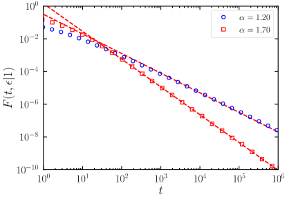
Figure 2: Distribution of the first passage time for a directed passive random walk on an infinitely aged NoPAD network, $F(t,c|c_{0})$, with inter-event time distribution given by Eq. (39), for different values of the exponent $\alpha$. We consider a bi-valued activity distribution with $c=\epsilon$ (with $\eta(\epsilon)=p$) or $c=1$ (with $\eta(1)=1-p$). We plot the first passage time distribution to nodes with $c=\epsilon$, with the walker starting from nodes with $c_{0}=1$ (hollow symbols), along with the expected behavior $F(t,c|c_{0})\sim t^{-\alpha}$ (dashed lines). Number of walkers $W=10^{6}$, $p=0.5$, $\epsilon=0.1$. Network size $N=10^{5}$.

VI Non-Poissonian Activity-Driven networks with infinite average inter-event time

We consider now an inter-event time distribution of the form Eq. (39) with $0<\alpha<1$, which implies that the average time between two consecutive activation of an agent with activity $c$ is infinite. For such values of $\alpha$, the dependency of the forward waiting time distribution on the aging time cannot be eliminated even in the limit of strongly aged networks, so that the use of the Laplace transform does not yield any substantial simplification. Nevertheless, some insight may be obtained concerning the dynamics of the random walk starting on a strongly aged network.

Let us recall the expression of the double Laplace transform of the forward waiting time distribution, namely Klafter and Sokolov (2011); Schulz et al. (2014); Barkai and Cheng (2003); Godrèche and Luck (2001),

$$h_{c}(u,s) = \int_{0}^{\infty}dt\int_{0}^{\infty}dt^{\prime}h_{c}(t^{\prime},t)e^{-ut^{\prime}}e^{-st}$$ (52)

$$= \frac{1}{1-\psi_{c}(u)}\frac{\psi_{c}(u)-\psi_{c}(s)}{s-u}.$$

Let us first consider the limit of strongly aged network and very large $t$, with $ct\gg ct_{a}\gg 1$, corresponding to $s\ll u\ll 1$. In this case, one can expand

$$h_{c}(u,s)\simeq\frac{u^{\alpha}-s^{\alpha}}{u^{1+\alpha}},$$ (53)

which, upon inverse transformation, leads to

$$h_{c}(t_{a},t)\simeq t_{a}^{\alpha}\;\frac{\sin(\pi\alpha)}{\pi}\;t^{-\alpha-1}.$$ (54)

On the other hand, in the limit of strong aging, $ct_{a}\gg 1$, but small $t\ll t_{a}$, one can expand $\psi_{c}(u)\sim 1+\alpha\Gamma_{-\alpha}u^{\alpha}c^{-\alpha}$ in Eq. (52) to obtain

$$h_{c}(u,s)\simeq-\frac{1}{s}-\frac{1-\psi_{c}(s)}{s\alpha\Gamma_{-\alpha}u^{\alpha}c^{-\alpha}},$$ (55)

which, disregarding a constant term, leads to

$$h_{c}(t_{a},t)\simeq c\,(c\,t_{a})^{\alpha-1}\;\frac{\sin(\pi\alpha)}{\pi}\;\tilde{\psi}_{c}(t),$$ (56)

where $\tilde{\psi}_{c}(t)=\int_{t}^{\infty}\psi_{c}(t^{\prime})\,dt^{\prime}=(ct+1)^{-\alpha}$. The behavior of $\tilde{\psi}_{c}(t)$ can be approximated to $\tilde{\psi}_{c}(t)\simeq 1$ if $ct\ll 1$, while for $ct\gg 1$, it holds $\tilde{\psi}_{c}(t)\simeq(ct)^{-\alpha}$. The behavior of $h_{c}(t_{a},t)$ can thus be summarized in the following three regimes:

$$h_{c}(t_{a},t)\simeq\left\{\begin{array}[]{ll}\frac{\sin(\pi\alpha)}{\pi}\;c\,(c\,t_{a})^{\alpha-1}&\mathrm{for}\;c\,t\ll 1\\ \frac{\sin(\pi\alpha)}{\pi}\;t_{a}^{\alpha-1}\;t^{-\alpha}&\mathrm{for}\;\;1\ll c\,t\ll c\,t_{a}\\ \frac{\sin(\pi\alpha)}{\pi}\;t_{a}^{\alpha}\;t^{-\alpha-1}&\mathrm{for}\;t\gg t_{a}\end{array}\right..$$ (57)

Interestingly, at large times, i.e. $ct\gg 1$, the forward waiting time distribution is independent of $c$. Besides, the tail of the distribution is proportional to $t_{a}^{\alpha}\,t^{-\alpha-1}$, so that the probability that the forward waiting time is greater than $t_{a}$ is constant and does not depend on $t_{a}$. This means that the interval $[t_{a},+\infty[$ carries a constant probability weight with respect to the other two terms, although its size decreases when $t_{a}$ grows. This, along with the fact that the total weight is constant and equal to $1$ because $h_{c}$ is normalized, implies that the weight carried in a time window $[0,t_{0}]$ tends to zero when $t_{a}$ tends to infinity. In fact, one could argue that the weights calculated from Eq. (57) are not exact because they neglect higher order corrections (in particular the distribution in Eq. (57) is not normalized). The reasoning is thus true under the implicit assumption that the weights calculated from Eq. (57) and carried in the intervals $[0,t_{0}]$ and $[t_{0},+\infty[$ are proportional to their corresponding real weights, which is not guaranteed.

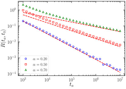
Figure 3: Ratios $R(t_{a},t_{0})=[\tilde{h}_{c}(t_{a},0)-\tilde{h}_{c}(t_{a},t_{0})]/\,\tilde{h}_{c}(t_{a},t_{0})$ as a function of $t_{a}$, obtained from numerical simulations of a renewal process with an inter-event time distribution of the form Eq. (39) with different values of $\alpha$. The asymptotes $\alpha(t_{0}/t_{a})^{1-\alpha}$ calculated from Eq. (57) are plotted as dashed lines. Reference time $t_{0}=10^{3}$ and $c=1$.

In order to check these assumptions, on Fig. 3 we compare the ratio of the real weights $R(t_{a},t_{0})\equiv\left[\tilde{h}_{c}(t_{a},0)-\tilde{h}_{c}(t_{a},t_{0})\right]/\,\tilde{h}_{c}(t_{a},t_{0})$, evaluated from a numerical simulation of a renewal process with an inter-event time distribution of the form Eq. (39), and the ratio evaluated from Eq. (57), whose dominant order, with the conditions $1\ll ct_{0}\ll ct_{a}$, is equal to $\alpha(t_{0}/t_{a})^{1-\alpha}$. We observe a good agreement between the simulations and the analytical estimation, which allows us to make the following reasoning: let us consider a NoPAD network with inter-event time distribution given by Eq. (39) with $\alpha<1$, and an arbitrary activity distribution $\eta(c)$ excluding zero-valued activities. Then there exists a node with a minimum activity $c_{\mathrm{min}}>0$, and also a time $t_{0}$, such that $c_{\mathrm{min}}\,t_{0}\gg 1$. Then if the nodes are synchronized at $t=-t_{a}$ with $t_{a}\gg t_{0}$ and we start an activated random walk dynamics at time $t=0$, the probability that the time $t_{1}$ at which the walkers escape from their first hosts is greater than $t_{0}$ is almost equal to $1$. This holds a fortiori for all the following waiting times of the walker occurring at times $t=t_{2},t_{3},...,t_{k}$ because $t_{k}$ is extracted from the distribution $h_{c}(t_{a}+t_{k-1},\tau)$. Besides, the conditional probability that $t_{1}=\tau$ given that $t_{1}\geq t_{0}$ is independent of $c$ as we see from Eq. (57), which means that all the hops for all the walkers are performed with waiting times that practically do not depend on the activity of the hosts.

As a result, after its first jump, the probability that a walker is at a node of activity $c$ is constant and equal to $\eta(c)$. In other words, if the initial distribution of the walkers is $H(c)$, the probability $P(c,t)$ that the walker is at a node with activity $c$ at time $t$ is equal to $\eta(c)$ if the walker has escaped from its first host and $H(c)$ otherwise, i.e.

$$P(c,t)\simeq H(c)\tilde{h}_{c}(t_{a},t)+\eta(c)(1-\tilde{h}_{c}(t_{a},t)).$$ (58)

In the limit of infinite $t$, $\tilde{h}_{c}(t_{a},t)$ vanishes, and the steady state of the walker is given by $P_{\infty}(c)=\eta(c)$. That is, in the large time regime, the walker behaves as in a completely homogeneous network, in which jumps were performed independently of the node activity. This result generalizes the observation made in Ref. Speidel et al. (2015).

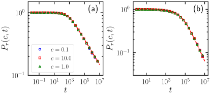
Figure 4: Random walk dynamics on an aged NoPAD network with three-valued activity and infinite average waiting time. Activity values are $c=0.1$, $c=1$ and $c=10$, with $\eta(c)=1/3$. Initial distribution $H(c)=\delta_{c,10}$. We plot for the three values of $c$ the reduced occupation probability $P_{r}(c,t)=(P(c,t)-\eta(c))/(H(c)-\eta(c))$ as a function of time. (a): $\alpha=0.2$ and $t_{a}=10^{3}$. (b): $\alpha=0.5$ and $t_{a}=10^{5}$. The behavior predicted by Eq. (58) is plotted in dashed lines. Network size $N=10^{5}$ and number of walkers $W=10^{6}$.

In order to check the validity of the time dependence expressed in Eq. (58), we have performed numerical simulations of the activated random walk on a NoPAD network of size $N=10^{5}$ where the activity takes three values, $c=0.1,1$ or $10$, each with probability $\eta(c)=1/3$. Walkers are initially hosted by nodes with activity equal to $c=10\;$, i.e. $H(c)=\delta_{c,10}$. Fig. 4 shows the reduced occupation probability $P_{r}(c,t)=[P(c,t)-\eta(c)]/[H(c)-\eta(c)]\;$ as a function of the time $t$ for $\alpha=0.2$ and $t_{a}=10^{3}$, Fig. 4(a), and for $\alpha=0.5$ and $t_{a}=10^{5}$, Fig. 4(b), along with their expected value $\tilde{h}_{c}(t_{a},t)$. This last curve is evaluated from an independent numerical simulation of a renewal process, and is found to be independent of the activity $c$. We observe that the result stated in Eq. (58) perfectly match the numerical simulations in networks of finite size.

VII Conclusions

In this paper we have explored the behavior of a passive node-centric random walk unfolding on non-Markovian temporal networks generated by the NoPAD model, which considers a power-law form $\psi_{c}(t)\sim(ct+1)^{-1-\alpha}$ of the inter-event time distribution between consecutive activation events of nodes with activity $c$. We have focused in particular on the behavior of the occupation probability and first passage time distribution, in the case of a very large aging time $t_{a}$, that is, when the time elapsed between the initial synchronization of all nodes in the network and the start of the random walker is very large. The nature of the NoPAD model allows to simplify calculations in the limit of infinite network size, in which every node in the path of the walker is visited for the first time. In this approximation, we develop a general theory for the walker dynamics, that can be analytically solved in Laplace space if the inter-event time distribution of the nodes has a finite first moment. In this case, in the limit $t_{a}\to\infty$, the waiting time of the walker inside a node becomes independent of its arrival time, and a passive random walk with inter-event time distribution $\phi_{c}(t)\sim t^{-1-\alpha}$, with $\alpha>1$, behaves essentially as a active random walk with $\phi_{c}(t)\sim t^{-\alpha}$, in which the internal clock of each node is reset after the lading of the walker. Numerical simulations show that the actual passive random walk process is very well described by our theory for a sufficiently large network size.

If the inter-event time distribution lacks a first moment, which happens in the case $\alpha<1$, our theory is not valid, since the waiting time inside a node cannot be decoupled from the landing time. In the limit of very large $t_{a}$, however, we develop arguments hinting that the random walker will “feel” a network with homogeneous activity distribution, which implies that the probability that the walker is at a node of activity $c$ is equal to $\eta(c)$ in the large time limit. This result is straightforwardly extended to arbitrary aging times $t_{a}$ (including non-aged networks $t_{a}=0$) because after a transient regime of duration $t^{\prime}$, the forward waiting time distribution $h_{c}(t_{a}+t^{\prime},\tau)$ will meet the conditions expressed in Eq. (57), and the system will be in the same situation as before, i.e. evolving as if the network was homogeneous. This observation generalizes the results in Ref. Speidel et al. (2015) referred to networks with identical inter-event time for all nodes. Interestingly, this result is also recovered taking the limit $\alpha\to 1$ in the equation describing the occupation probability in the case of an inter-event time distribution with finite first moment, a fact that provides additional evidence for its relevance.

References

- Holme (2015) P. Holme, The European Physical Journal B 88, 234 (2015).
- Lambiotte and Masuda (2016) R. Lambiotte and N. Masuda, A Guide to Temporal Networks, Series On Complexity Science, Vol. 4 (World Scientific, Singapore, 2016).
- Newman (2010) M. E. J. Newman, Networks: An introduction (Oxford University Press, Oxford, 2010).
- Gauvin et al. (2018) L. Gauvin, M. Génois, M. Karsai, M. Kivelä, T. Takaguchi, E. Valdano, and C. L. Vestergaard, CoRR abs/1806.04032 (2018).
- Perra et al. (2012a) N. Perra, B. Gonçalves, R. Pastor-Satorras, and A. Vespignani, Scientific reports 2, 469 (2012a).
- Starnini and Pastor-Satorras (2013) M. Starnini and R. Pastor-Satorras, Physical Review E 87, 062807 (2013).
- Perra et al. (2012b) N. Perra, A. Baronchelli, D. Mocanu, B. Gonçalves, R. Pastor-Satorras, and A. Vespignani, Physical Review Letters 109, 238701 (2012b).
- Starnini and Pastor-Satorras (2014) M. Starnini and R. Pastor-Satorras, Physical Review E 89, 032807 (2014).
- Liu et al. (2014) S. Liu, N. Perra, M. Karsai, and A. Vespignani, Phys. Rev. Lett. 112, 118702 (2014).
- Alessandretti et al. (2017) L. Alessandretti, K. Sun, A. Baronchelli, and N. Perra, Phys. Rev. E 95, 052318 (2017).
- Pozzana et al. (2017) I. Pozzana, K. Sun, and N. Perra, Phys. Rev. E 96, 042310 (2017).
- Nadini et al. (2018) M. Nadini, K. Sun, E. Ubaldi, M. Starnini, A. Rizzo, and N. Perra, Scientific Reports 8, 2352 (2018).
- Onnela et al. (2007) J.-P. Onnela, J. Saramäki, J. Hyvönen, G. Szabó, D. Lazer, K. Kaski, J. Kertész, and A.-L. Barabási, Proceedings of the National Academy of Sciences 104, 7332 (2007).
- Cattuto et al. (2010) C. Cattuto, W. Van den Broeck, A. Barrat, V. Colizza, J.-F. Pinton, and A. Vespignani, PLoS ONE 5, e11596 (2010).
- Corral (2004) A. Corral, Phys. Rev. Lett. 92, 108501 (2004).
- Wheatland et al. (1998) M. S. Wheatland, P. A. Sturrock, and J. M. McTiernan, The Astrophysical Journal 509, 448+ (1998).
- Kemuriyama et al. (2010) T. Kemuriyama, H. Ohta, Y. Sato, S. Maruyama, M. Tandai-Hiruma, K. Kato, and Y. Nishida, Biosystems 101, 144 (2010).
- Barabàsi (2005) A.-L. Barabàsi, Nature 435, 207 (2005).
- Holme (2003) P. Holme, Europhys. Lett. 64, 427 (2003).
- Moinet et al. (2015) A. Moinet, M. Starnini, and R. Pastor-Satorras, Phys. Rev. Lett. 114, 108701 (2015).
- Karsai et al. (2014) M. Karsai, N. Perra, and A. Vespignani, Sci Rep 4, 4001 (2014).
- Vestergaard et al. (2014) C. L. Vestergaard, M. Génois, and A. Barrat, Phys. Rev. E 90, 042805 (2014).
- García-Pérez et al. (2015) G. García-Pérez, M. Boguñá, and M. Á. Serrano, Scientific Reports 5, 9714 EP (2015).
- Jo et al. (2014) H.-H. Jo, J. I. Perotti, K. Kaski, and J. Kertész, Physical Review X 4, 011041 (2014).
- Kiss et al. (2015) I. Z. Kiss, G. Röst, and Z. Vizi, Phys. Rev. Lett. 115, 078701 (2015).
- Scholtes et al. (2014) I. Scholtes, N. Wider, R. Pfitzner, A. Garas, C. J. Tessone, and F. Schweitzer, Nature Communications 5, 5024 EP (2014).
- Van Mieghem and van de Bovenkamp (2013) P. Van Mieghem and R. van de Bovenkamp, Physical Review Letters 110 (2013), 10.1103/PhysRevLett.110.108701.
- Starnini et al. (2017) M. Starnini, J. P. Gleeson, and M. Boguñá, Phys. Rev. Lett. 118, 128301 (2017).
- Boguñá et al. (2014) M. Boguñá, L. F. Lafuerza, R. Toral, and M. A. Serrano, Phys. Rev. E 90, 042108 (2014).
- Sun et al. (2015) K. Sun, A. Baronchelli, and N. Perra, Eur. Phys. J. B 88, 326 (2015).
- Moinet et al. (2016) A. Moinet, M. Starnini, and R. Pastor-Satorras, Phys. Rev. E 94, 022316 (2016).
- Porter and Gleeson (2016) M. Porter and J. Gleeson, Dynamical Systems on Networks: A Tutorial, Frontiers in Applied Dynamical Systems: Reviews and Tutorials, Vol. 4 (Springer International Publishing, Switzerland, 2016).
- Weiss (1994) G. H. Weiss, Aspects and Applications of the Random Walk (North-Holland Publishing Co., Amsterdam, 1994).
- Masuda et al. (2017) N. Masuda, M. A. Porter, and R. Lambiotte, Physics Reports 716-717, 1 (2017).
- Klafter and Sokolov (2011) J. Klafter and I. Sokolov, First Steps in Random Walks: From Tools to Applications (Oxford University Press, Oxford, 2011).
- Cox (1967) D. R. Cox, Renewal Theory (Methuen, London, 1967).
- Sousa da Mata and Pastor-Satorras (2015) A. Sousa da Mata and R. Pastor-Satorras, The European Physical Journal B 88, 12 (2015), 10.1140/epjb/e2014-50801-1.
- Schulz et al. (2014) J. H. Schulz, E. Barkai, and R. Metzler, Physical Review X 4, 011028 (2014).
- Speidel et al. (2015) L. Speidel, R. Lambiotte, K. Aihara, and N. Masuda, Physical Review E 91, 012806 (2015).
- Hoffmann et al. (2012) T. Hoffmann, M. A. Porter, and R. Lambiotte, Physical Review E 86, 046102 (2012).
- de Nigris et al. (2016) S. de Nigris, A. Hastir, and R. Lambiotte, The European Physical Journal B 89, 114 (2016).
- Lambiotte et al. (2013) R. Lambiotte, L. Tabourier, and J.-C. Delvenne, Eur. Phys. J. B 86, 320 (2013).
- Abramowitz and Stegun (1972) M. Abramowitz and I. A. Stegun, Handbook of mathematical functions. (Dover, New York, 1972).
- Barkai and Cheng (2003) E. Barkai and Y.-C. Cheng, J. Chem. Phys. 118, 6167 (2003).
- Godrèche and Luck (2001) C. Godrèche and J. Luck, Journal of Statistical Physics 104, 711 (2001).