Neural Logic Reinforcement Learning

Abstract

Deep reinforcement learning (DRL) has achieved significant breakthroughs in various tasks. However, most DRL algorithms suffer a problem of generalising the learned policy, which makes the policy performance largely affected even by minor modifications of the training environment. Except that, the use of deep neural networks makes the learned policies hard to be interpretable. To address these two challenges, we propose a novel algorithm named Neural Logic Reinforcement Learning (NLRL) to represent the policies in reinforcement learning by first-order logic. NLRL is based on policy gradient methods and differentiable inductive logic programming that have demonstrated significant advantages in terms of interpretability and generalisability in supervised tasks. Extensive experiments conducted on cliff-walking and blocks manipulation tasks demonstrate that NLRL can induce interpretable policies achieving near-optimal performance while showing good generalisability to environments of different initial states and problem sizes.

1 Introduction

In recent years, Deep Reinforcement Learning (DRL) algorithms have achieved stunning breakthroughs in vairous tasks, e.g., video game playing (Mnih et al., 2015) and the game of Go (Silver et al., 2017). However, similar to traditional reinforcement learning algorithms such as tabular TD-learning (Sutton & Barto, 1998), DRL algorithms can only learn policies that are hard to interpret (Montavon et al., ) and cannot be generalized from one environment to another similar one (Wulfmeier et al., 2017).

(Doshi-Velez & Kim, 2017) defines interpretability as the ability to explain or to present the decision in understandable terms. The interpretability is a critical capability of reinforcement learning or generally all machine learning algorithms for system verification and improvement. Interpretable RL can promote the scientific understanding of the algorithm or the problem to be solved. Furthermore, we can check whether an AI system is safe and whether it complies with existing rules, ethnically or legally, in human society. On the engineering level, the interpretability also enables easier debugging of the system. The neural network based DRL models, however, lack interpretability since the inference processes of neural networks are opaque to humans.

The generalizability is also important for reinforcement learning algorithms. In the real world, it is not common that the training and test environments are exactly the same. However, most DRL algorithms have the assumption that these two environments are identical, which makes a trained network that performs well on one task often performs very poorly on a new but similar task. An exampleis the reality gap (Collins et al., 2018) in the robotics applications that often makes agents trained in simulation ineffective once transferred in the real world.

The generalization of DRL policy is a rather intricate and difficult problem since the action can affect the environment dynamics. In supervised learning, there are regularization techniques such as Dropout (Srivastava et al., 2014) that can help to promote generalization. However, (Zhang et al., 2018) shows that noise injection methods used in several DRL works cannot robustly detect or alleviate overfitting. On the other hand, it is good to see that, similar to the supervised learning, a proper inductive bias that fits the problem bias can significantly improve the generalizability of the learned policies (Zhang et al., 2018). One candidate of inductive bias suitable for general decision-making is the relational inductive bias (Zambaldi et al., 2018). Relational inductive bias usually represents the abstract concepts as entities and relationships between them and perform deduction on the relations. The graph-based relational inductive bias has been tested in RL context (Zambaldi et al., 2018; Wang et al., 2018) and showed significantly better generalization compared with Multilayer Perceptron (MLP) architectures or Convoluational Neural Networks (CNNs). However, another more expressive relational inductive, i.e., the one based on first-order logic, is still not much explored by the DRL community.

The traditional symbolic methods intrinsically have good interpretable and generalizable capabilities, however, require the systems dynamics to be known and ideally deterministic when solving general sequential decision-making problems (Fikes & Nilsson, 1971). By contrast, relational reinforcement learning (Džeroski et al., 2001) learns first-order logic rules in some simple block manipulation tasks without the knowledge of system dynamics, and also shows good generalizability and interpretability on these tasks. However, such methods become ineffective when applied to more complex tasks, especially given that the symbolic learning methods have poor scalability.

A spectrum of such interpretable neural architectures is Differentiable Inductive Logic Programming (DILP) (Rocktäschel & Riedel, 2017; Cohen et al., 2017; Evans & Grefenstette, 2018). Compared with traditional symbolic logic induction methods, with the use of differentiable models, DILP can leverage modern gradients based methods. On the other side, thanks to the strong relational inductive bias, DILP shows superior interpretability and generalization ability than neural networks (Evans & Grefenstette, 2018). However, to the authors’ best knowledge, all current DILP algorithms are only tested in supervised tasks such as hand-crafted concept learning (Evans & Grefenstette, 2018) and knowledge base completion (Rocktäschel & Riedel, 2017; Cohen et al., 2017).

To make a step further, in this paper we develop a novel framework named as Neural Logic Reinforcement Learning (NLRL) to enable the differentiable induction in sequential decision-making tasks. It can alleviate the interpretability and generalizability problems in deep reinforcement learning. In addition, the proposed NLRL framework is also of great significance in advancing the DILP research. By applying DILP in sequential decision-making tasks, the agents can learn new concepts without human supervision, instead of describing a concept already known to the human in supervised learning tasks.

The rest of the paper is organized as follows: In Section 2, related works are reviewed and discussed; In Section 3, an introduction to the preliminary knowledge is presented, including the first-order logic programming $\partial$ILP and Markov Decision Processes (MDPs); In Section 4, the NLRL model is introduced, both the DILP architecture and a general NLRL framework modeled with MDPs; In Section 5, the experiments of NLRL on block manipulation and cliff-walking are presented; In the last section, the paper is concluded and future directions are directed.

2 Related Work

We place our work in the development of relational reinforcement learning (Džeroski et al., 2001) that represent states, actions and policies in Markov Decision Processes (MDPs) using the first order logic where transitions and rewards structures of MDPs are unknown to the agent. To this end, in this section we review the evolution of relational reinforcement learning and highlight the differences of our proposed NLRL framework with other algorithms in relational reinforcement learning.

Early attempts that represent states by first-order logics in MDPs appeared at the beginning of this century (Boutilier et al., 2001; Yoon et al., 2002; Guestrin et al., 2003), however, these works focused on the situation that transitions and reward structures are known to the agent. In such cases with environment models known, variations of traditional MDP solvers such as dynamic programming (Boutilier et al., 2001), linear programming (Guestrin et al., 2003) and heuristic greedy searching (Yoon et al., 2002) were employed to optimise policies in training tasks that can be generalized to large problems. In these works, the transition and reward functions are also represented in logic forms. The setting limits their application to complex tasks whose transition and reward functions are hard to be modeled using the first order logic.

The concept of relational reinforcement learning was first proposed by (Džeroski et al., 2001) in which the first order logic was first used in reinforcement learning. There are extensions of this work (Driessens & Ramon, 2003; Driessens & Džeroski, 2004), however, all these algorithms employ non-differential operations, which makes it hard to apply new breakthroughs happened in DRL community. In contrast, in our work using differentiable inductive logic programming, once given the logic interpretations of states and actions, any type of MDPs can be solved with policy gradient methods compatible with DRL algorithms. Furthermore, most relational reinforcement learning algorithms represent the induced policy in a single clause and some auxiliary predicates, e.g., the predicates that count the number of blocks, are given to the agent. In our work, the DILP algorithms have the ability to learn the auxiliary invented predicates by the agents themselves, which not only enables stronger expressive ability but also gives possibilities for knowledge transfer.

One previous work close to ours is (Gretton, 2007) that also trains the parameterised rule-based policy using policy gradient. An approach was proposed to pre-construct a set of potential policies in a brutal force manner and train the weights assigned to them using policy gradient. Compared to this work, in our NLRL framework weights are not assigned directly to the whole policy; the parameters to be trained are involved in the deduction process and the number of parameters is significantly smaller than that in an enumeration of all policies, especially for larger problems, which gives our method better scalability. In addition, in (Gretton, 2007), expert domain knowledge is needed to specify the potential rules for the exact task that the agent is dealing with. However, in our work, we use the same rules templates for all tasks we test on, which means all the potential rules have the same format across tasks.

A recent work on the topic (Zambaldi et al., 2018) proposes deep reinforcement learning with relational inductive bias that applies neural network mixed with self-attention to reinforcement learning tasks and achieves the state-of-the-art performance on the StarCraftII mini-games. The proposed methods show some level of generalization ability on the constructed block world problems and StarCraft mini-games, showing the potential of relation inductive bias in larger problems. However, as a graph-based relational model was used (Zambaldi et al., 2018), the learned policy is not fully explainable and the rules expression is limited, different from the interpretable logic-represented policies learned in ours using DILP.

A parallel work (Dong et al., 2019) use neural networks to approximate the first-order logic deduction, achieving good generalization on both supervised and reinforcement learning tasks. Their method has better scalibility than DILP based approaches, however, it is still not clear how to interpret the policies learned by their model.

3 Preliminary

In this section, we give a brief introduction to the necessary background knowledge of the proposed NLRL framework. Basic concepts of the first-order logic are first introduced. $\partial$ILP, a DILP model that our work is based on, is then described. The Markov Decision Process (MDP) and reinforcement learning are also briefly introduced.

3.1 First-Order Logic Programming

Logic programming languages are a class of programming languages using logic rules rather than imperative commands. One of the most famous logic programming languages is ProLog, which expresses rules using the first-order logic. In this paper, we use the subset of ProLog, i.e., DataLog (Getoor & Taskar, 2007).

Predicate names (or for short, predicates), constants and variables are three primitives in DataLog. In the language of relational learning, a predicate name is also called a relation name, and a constant is also termed as an entity (Getoor & Taskar, 2007). An atom $\alpha$ is a predicate followed by a tuple $p(t_{1},...,t_{n})$, where $p$ is an n-ary predicate and $t_{1},...,t_{n}$ are terms, either variables or constants. For example, in the atom father(cart, Y), father is the predicate name, cart is a constant and Y is a variable. If all terms in an atom are constants, this atom is called a ground atom. We denote the set of all ground atoms as $G$. A predicate can be defined by a set of ground atoms, in which case the predicate is called an extensional predicate. Another way to define a predicate is to use a set of clauses. A clause is a rule in the form $\alpha\leftarrow\alpha_{1},...,\alpha_{n}$, where $\alpha$ is the head atom and $\alpha_{1},...,\alpha_{n}$ are body atoms. The predicates defined by clauses are termed as intensional predicates.

3.2 $\partial$ILP

Inductive logic programming (ILP) is a task to find a definition (set of clauses) of some intensional predicates, given some positive examples and negative examples (Getoor & Taskar, 2007). The attempts that combine ILP with differentiable programming are presented in (Evans & Grefenstette, 2018; Rocktäschel & Riedel, 2017) and $\partial$ILP (Evans & Grefenstette, 2018) is introduced here that our work is based on.

The major component of $\partial$ILP operates on the valuation vectors $\boldsymbol{e}$ whose space is $E=[0,1]^{|G|}$, where each element of a valuation vector represents the confidence that a related ground atom is true. The logical deduction of each step of the $\partial$ILP is applied to the valuation vector. The new facts are derived from the facts provided by the valuation vector in the last step. For each predicate, $\partial$ILP generates a series of potential clauses combinations in advance based on rules templates. Trainable weights are assigned to clauses combinations, and the sum of weights for a predicate is constrained to be summed up to 1 using a softmax function.

With the differentiable deduction, the system can be trained with gradient-based methods. The loss value is defined as the cross-entropy between the confidence of predicted atoms and the ground truth. Compared with traditional inductive logic programming methods, $\partial$ILP has advantages in terms of robustness against noise and ability to deal with fuzzy data (Evans & Grefenstette, 2018).

4 Neural Logic Reinforcement Learning

In this section, the details of the proposed NLRL framework are presented. A new DILP architecture termed as Differentiable Recurrent Logic Machine (DRLM), an improved version of $\partial$ILP, is first introduced. The MDP with logic interpretation is then proposed to train the DILP architecture.

4.1 Differentiable Recurrent Logic Machine

Recall that $\partial$ILP operates on the valuation vectors whose space is $E=[0,1]^{|G|}$, each element of which represents the confidence that a related ground atom is true. A DRLM is a mapping $f_{\boldsymbol{\theta}}:E\to E$, which performs the deduction of the facts $\boldsymbol{e}_{0}$ using weights $\boldsymbol{w}$ associated with possible clauses. $f_{\boldsymbol{\theta}}$ can then be decomposed into repeated application of single step deduction functions $g_{\boldsymbol{\theta}}$, namely,

$$f_{\boldsymbol{\theta}}^{t}(\boldsymbol{e}_{0})=\begin{cases}g_{\boldsymbol{\theta}}(f_{\boldsymbol{\theta}}^{t-1}(\boldsymbol{e}_{0})),&\text{if $t>0$}.\\ \boldsymbol{e}_{0},&\text{if $t=0$}.\end{cases}\text{,}$$ (1)

where $t$ is the deduction step. $g_{\boldsymbol{\theta}}$ implements one step deduction of all the possible clauses weighted by their confidences. We denote the probabilistic sum as $\oplus$ and

$$\boldsymbol{a}\oplus\boldsymbol{b}=\boldsymbol{a}+\boldsymbol{b}-\boldsymbol{a}\odot\boldsymbol{b}\text{,}$$ (2)

where $\boldsymbol{a}\in E,\boldsymbol{b}\in E$. $g_{\boldsymbol{\theta}}$ can then be expressed as

$$g_{\boldsymbol{\theta}}(\boldsymbol{e})=\left(\sum_{n}^{\oplus}\sum_{j}w_{n,j}h_{n,j}(\boldsymbol{e})\right)+\boldsymbol{e}_{0}\text{,}$$ (3)

where $h_{n,j}(\boldsymbol{e})$ implements one-step deduction of the valuation vector $\boldsymbol{e}$ using $j$th possible definition of $n$th clause. For every single clause $c$, we can constrain the sum of its weights to be 1 by letting $\boldsymbol{w}_{c}=\text{softmax}(\boldsymbol{\theta}_{c})$, where $\boldsymbol{w}_{c}$ is the vector of weights associated with the predicate $c$ and $\boldsymbol{\theta}_{c}$ are related parameters to be trained.

Compared to $\partial$ILP, in DRLM the number of clauses used to define a predicate is more flexible thanks to associating the weights with clauses directly instead of combinations of clauses; it needs less memory to construct a model (less than 10 GB in all our experiments); it also enables learning longer logic chaining of different intensional predicates. All these benefits make the architecture be able to work in larger problems. Detailed discussions on the modifications and their effects can be found in the appendix.

4.2 Markov Decision Process with Logic Interpretation

In this section, we present a formulation of MDPs with logic interpretation and show how to solve the MDP with the combination of policy gradient and DILP.

An MDP with logic interpretation is a triple $(M,p_{S},p_{A})$:

• $M=(S,A,T,R)$ is a finite-horizon MDP;

• $p_{S}:S\to 2^{G}$ is the state encoder that maps each state to a set of atoms including both information of the current state and background knowledge;

• $p_{A}:[0,1]^{|D|}\to[0,1]^{|A|}$ is the action decoder that maps the valuation (or score) of a set of atoms $D$ to the probability of actions.

For a DILP system $f_{\boldsymbol{\theta}}:2^{G}\to[0,1]^{|D|}$, the policy $\pi:S\to[0,1]^{|D|}$ can be expressed as $\pi(s)=p_{A}(f_{\boldsymbol{\theta}}(p_{S}(s)))$. Thus any policy-gradient methods applied to DRL can also work for DILP. $p_{S}$ and $p_{A}$ can either be hand-crafted or represented by neural architectures. The action selection mechanism in this work is to add a set of action predicates into the architecture, which depends on the valuation of these action atoms. Therefore, the action atoms should be a subset of $D$. As for $\partial$ILP, valuations of all the atoms will be deduced, i.e., $D=G$. If $p_{S}$ and $p_{A}$ are neural architectures, they can be trained together with the DILP architectures. $p_{S}$ extracts entities and their relations from the raw sensory data. In addition, the use of a neural network to represent $p_{A}$ enables agents to make decisions in a more flexible manner. For instance, the output actions can be deterministic and the final choice of action may depend on more atoms rather than only action atoms if the optimal policy cannot be easily expressed as first-order logic. For simplicity, in this work, we will only use the hand-crafted $p_{S}$ and $p_{A}$. Notably, $p_{A}$ is required to be differentiable so that we can train the system with policy gradient methods operating on discrete, stochastic action spaces, such as vanilla policy gradient (Willia, 1992), A3C (Mnih et al., 2016), TRPO (Schulman et al., 2015a) or PPO (Schulman et al., 2017).

We use the following schema to represent the $p_{A}$ in all experiments. Let $p_{A}(a|\boldsymbol{e})$ be the probability of choosing action $a$ given the valuations $\boldsymbol{e}\in[0,1]^{|D|}$. The probability of choosing an action $a$ is proportional to its valuation if the sum of the valuation of all action atoms is larger than 1; otherwise, the difference between 1 and the total valuation will be evenly distributed to all actions, i.e.,

$$p_{A}(a|\boldsymbol{e})=\begin{cases}\frac{l(e,a)}{\sigma},&\sigma\geq 1\\ l(e,a)+\frac{1-\sigma}{|A|},&\sigma<1\end{cases}$$ (4)

where $l:[0,1]^{|D|}\times A\to[0,1]$ maps from valuation vector and action to the valuation of that action atom, $\sigma$ is the sum of all action valuations $\sigma=\sum_{a}l(e,a)$. Empirically, this design is crucial for inducing an interpretable and generalizable policy. If we apply a trivial normalization, it is not necessary for NLRL agent to increase rule weights to 1 for the sake of exploitation. The agent instead only needs to keep the relative valuation advantages of desired actions over other actions, which in practice leads to tricky policies. We train all the agents with vanilla policy gradient (Willia, 1992) in this work.

5 Experiments and Analysis

In general, the experiment is going to act as empirical investigations of the following hypothesis:

1. NLRL can learn policies that are comparable to neural networks in terms of expected returns;

2. To induce these policies, we only need to inject minimal background knowledge;

3. The induced policies are explainable;

4. The induced policies can generalize to environments that are different from the training environments in terms of scale or initial state.

Four sets of experiments, which are STACK, UNSTACK and ON block manipulation tasks, and cliff-walking, have been conducted and the benchmark model is a fully-connected neural network. The induced policy will be evaluated in terms of expected returns, generalizability and interpretability.

5.1 Experiment Setup

In the experiments, to test the robustness of the proposed NLRL framework, we only provide minimal atoms describing the background and states while the auxiliary predicates are not provided. The agent must learn auxiliary invented predicates by themselves, together with the action predicates.

5.1.1 Block Manipulation

In this environment, the agent will learn how to stack the blocks into certain styles, that are widely used as a benchmark problem in the relational reinforcement learning research. We examine the performance of the agent on three subtasks: STACK, UNSTACK and ON. In the STACK task, the agent needs to stack the scattered blocks into a single column. In the UNSTACK task, the agent needs to do the opposite operation, i.e., spread the blocks on the floor. In the ON task, it is required to put a specific block onto another one. In all three tasks, the agent can only move the topmost block in a pile of blocks. When the agent finishes its goal it will get a reward of 1; before that, the agent keeps receiving a small penalty of -0.02. The training is terminated if the agent does not reach the goal within 50 steps.

Figure 1: A Blocks Manipulation state noted as $((a,b,c),(d))$.

There are 5 different entities, 4 blocks labeled as a, b, c, d and floor. The state predicates are on(X,Y) and top(X). on(X,Y) means the block X is on the entity Y (either blocks or floor). $top(X)$ means the block $X$ is on top of an column of blocks. Notably, $top(X)$ cannot be expressed using $on$ here as in DataLog there is no expression of negation, i.e., it cannot have “$top(X)$ means there is no $on(Y,X)$ for all $Y$”. For all tasks, a common background knowledge is isFloor(floor), and for the ON task, there is one more background knowledge predicate goalOn(a,b), which indicates the target is to move block $a$ onto the block $b$. The action predicate is move(X,Y) and there are 25 actions atoms in this task. The action is valid only if both $Y$ and $X$ are on the top of a pile or $Y$ is $floor$ and $X$ is on the top of a pile. If the agent chooses an invalid action, e.g., move(floor, a), the action will not make any change to the state. We use a tuple of tuples to represent the states, where each inner tuple represents a column of blocks, from bottom to top. For instance, Figure 1 shows the state $((a,b,c),(d))$ and its logic representation.

The training environment of the UNSTACK task starts from a single column of blocks $((a,b,c,d))$. To test the generalizability of the induced policy, we construct the test environment by modifying its initial state by swapping the top 2 blocks or dividing the blocks into 2 columns. The agent is also tested in the environments with more blocks stacking in one column. Therefore, the initial states of all the generalization test of UNSTACK are: $((a,b,d,c))$, $((a,b),(c,d))$, $((a,b,c,d,e))$, $((a,b,c,d,e,f))$ and $((a,b,c,d,e,f,g))$. For the STACK task, the initial state is $((a),(b),(c),(d))$ in training environment. Similar to the UNSTACK task, we swap the right two blocks, divide them into 2 columns and increase the number of blocks as generalization tests. The initial states of all the generalization test of STACK are: $((a),(b),(d),(c))$, $((a,b),(d,c))$, $((a),(b),(c),(d),(e))$, $((a),(b),(c),(d),(e),(f))$, $((a),(b),(c),(d),(e),(f),(g))$. For ON, the initial state is $((a,b,c,d))$. We swap either the top two or middle two blocks in this case, and also increase the total number of blocks. The initial states of all the generalization test of ON are thus: $((a,b,d,c))$, $((a,c,b,d))$, $((a,b,c,d,e))$, $((a,b,c,d,e,f))$ and $((a,b,c,d,e,f,g))$.

5.1.2 Cliff-walking

Cliff-walking is a commonly used toy task for reinforcement learning. We modify the version in (Sutton & Barto, 1998) to a 5 by 5 field, as shown in Figure 2. When the agent reaches the cliff position it gets a reward of -1, and if the agent arrives at the goal position, it gets a reward of 1. Before reaching these absorbing positions, the agent keeps receiving a small penalty of -0.02 at each step, encouraged to reach the goal as soon as possible. If the agent fails to reach the absorbing states within 50 steps, the game will be terminated. This problem can be modelled as a finite-horizon MDP.

The constants in this experiment are integers from 0 to 4. We inject basic knowledge about natural numbers including the smallest number (zero(0)), largest number (last(4)), and the order of the numbers (succ(0,1), succ(1,2), …). The symbolic representation of the state is current(X,Y), which specifies the current position of the agent. There are four action atoms: up(), down(), left() and right().

In the training environment of cliff-walking, the agent starts from the bottom left corner, labelled as $S$ in Figure 2. In the generalization tests, we move the initial position to the top left, top right, and the centre of the field, labelled as $S_{1},S_{2}$ and $S_{3}$ respectively. Then we increase the size of the whole field to 6 by 6 and 7 by 7 without retraining.

We also test a stochastic variant of cliff-walking, i.e., windy cliff-walking, where the agent has a 10% chance to move downwards no matter which action it takes.

Figure 2: Cliff-walking, the circle represents location of the agent.

5.1.3 Hyperparameters

Similar to $\partial$ILP, we use RMSProp to train the agent, whose learning rate is set as 0.001. The generalized advantages ($\lambda=0.95$) (Schulman et al., 2015b) are applied to the value network where the value is estimated by a neural network with one 20-units hidden layer.

Like the architecture design to the neural network, the rules templates are important hyperparameters to the DILP algorithms. The rules template of a clause indicates the arity of the predicate (can be 0, 1, or 2) and the number of existential variables (usually pick from $\{0,1,2\}$). It also specifies whether the body of a clause can contain other invented predicates. We represent a rule template as a tuple of its three parameters, such as $(2,1,True)$, for the simplicity of expression. The rules templates of the DRLM are quite general and the optimal setting can be searched automatically. In this work, however, we use the same rules templates for invented predicates across all the tasks, each with only 1 clause, i.e., $(1,1,True),(1,2,False),(2,1,True),(2,1,True)$. The templates of action predicates vary in different tasks but it is easy to find a good one by exhaustive search. To this end, little domain knowledge is needed. For the UNSTACK and STACK tasks, the action predicate template is $(2,1,True)$. For the ON task, the action predicate templates are $(2,1,True)$ and $(2,0,True)$. There are four action predicates in the cliff-walking task, we give all these predicates the same template $(3,1,True)$.

5.1.4 Benchmark Neural Network Agent

In all the tasks, in addition to a random agent, we use an MLP agent as another benchmark that has two hidden layers with 20 units and 10 units respectively. All the units in the hidden layers use a ReLU (Nair & Hinton, 2010) activation function. For the cliff-walking task, the input is the coordinates of the current position of the agent. For block stacking tasks, the input is a $7\times 7\times 7$ tensor $X$, where $X_{x,y,i}=1$ if the block indexed as $i$ is in position $x,y$. We set each dimension of the tensor as 7 that is the maximum number of blocks used in the generalization test.

5.2 Results and Analysis

The performance of policy deduced by NLRL is stable against different random seeds once all the hyper-parameters are fixed, therefore, we only present the evaluation results of the policy trained in the first run for NLRL here. For the neural network agent, we pick the agent that performs best in the training environment out of 5 runs. The induced policy is also evaluated in terms of interpretability.

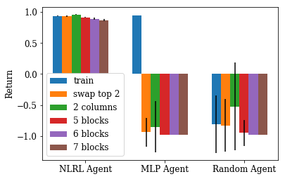
(a) UNSTACK

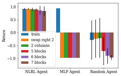
(b) STACK

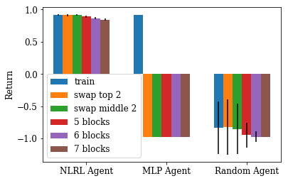
(c) ON

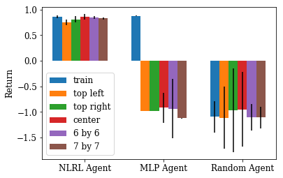
(d) Cliff-walking

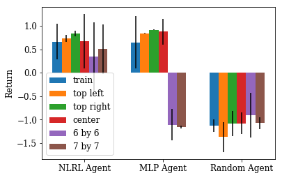
(e) Windy Cliff-walking

Figure 3: Performance of different agents in the training and test environments. Each sub-figure shows the performance of the three agents in a task. The performance of each agent is divided into a group. In each group, the blue bar shows the performance in the training environment while the others show the performance in the test environments.

Table 1: The returns of different agents in the training and test environments. The first three columns demonstrate the returns of the three agents; the last column shows the returns of the optimal policy, which is computed using value iteration.

		NLRL	MLP	Random	Optimal
UNSTACK	training	$0.937\pm 0.008$	$\mathbf{0.940}\pm 0.000$	$-0.807\pm 0.466$	$0.940$
	swap top 2	$\mathbf{0.936}\pm 0.009$	$-0.940\pm 0.232$	$-0.827\pm 0.428$	$0.940$
	2 columns	$\mathbf{0.958}\pm 0.006$	$-0.852\pm 0.414$	$-0.522\pm 0.710$	$0.960$
	5 blocks	$\mathbf{0.915}\pm 0.010$	$-0.980\pm 0.000$	$-0.948\pm 0.208$	$0.920$
	6 blocks	$\mathbf{0.891}\pm 0.014$	$-0.980\pm 0.000$	$-0.980\pm 0.000$	$0.900$
	7 blocks	$\mathbf{0.868}\pm 0.016$	$-0.980\pm 0.000$	$-0.980\pm 0.000$	$0.880$
STACK	training	$0.910\pm 0.033$	$\mathbf{0.940}\pm 0.000$	$-0.292\pm 0.759$	$0.940$
	swap right 2	$\mathbf{0.913}\pm 0.029$	$-0.980\pm 0.000$	$-0.240\pm 0.739$	$0.940$
	2 columns	$\mathbf{0.897}\pm 0.064$	$-0.980\pm 0.000$	$-0.215\pm 0.772$	$0.940$
	5 blocks	$\mathbf{0.891}\pm 0.032$	$-0.980\pm 0.000$	$-0.718\pm 0.542$	$0.920$
	6 blocks	$\mathbf{0.856}\pm 0.169$	$-0.980\pm 0.000$	$-0.905\pm 0.307$	$0.900$
	7 blocks	$\mathbf{0.828}\pm 0.179$	$-0.980\pm 0.000$	$-0.973\pm 0.097$	$0.880$
ON	training	$0.915\pm 0.01$	$\mathbf{0.920}\pm 0.000$	$-0.837\pm 0.405$	$0.920$
	swap top 2	$\mathbf{0.912}\pm 0.013$	$-0.980\pm 0.000$	$-0.821\pm 0.432$	$0.920$
	swap middle 2	$\mathbf{0.914}\pm 0.011$	$-0.980\pm 0.000$	$-0.853\pm 0.394$	$0.920$
	5 blocks	$\mathbf{0.890}\pm 0.016$	$-0.980\pm 0.000$	$-0.949\pm 0.195$	$0.900$
	6 blocks	$\mathbf{0.865}\pm 0.018$	$-0.980\pm 0.000$	$-0.975\pm 0.081$	$0.880$
	7 blocks	$\mathbf{0.844}\pm 0.017$	$-0.980\pm 0.000$	$-0.980\pm 0.000$	$0.860$
Cliff-walking	training	$0.862\pm 0.026$	$\mathbf{0.877}\pm 0.008$	$-1.096\pm 0.307$	$0.880$
	top left	$\mathbf{0.749}\pm 0.057$	$-0.980\pm 0.000$	$-1.115\pm 0.606$	$0.840$
	top right	$\mathbf{0.809}\pm 0.064$	$-0.980\pm 0.000$	$-0.966\pm 0.817$	$0.920$
	center	$\mathbf{0.859}\pm 0.05$	$-0.917\pm 0.296$	$-0.952\pm 0.730$	$0.920$
	6 by 6	$\mathbf{0.841}\pm 0.024$	$-0.934\pm 0.578$	$-1.101\pm 0.260$	$0.860$
	7 by 7	$\mathbf{0.824}\pm 0.024$	$-1.122\pm 0.006$	$-1.107\pm 0.209$	$0.840$
Windy Cliff-walking	training	$\mathbf{0.663}\pm 0.377$	$0.649\pm 0.558$	$-1.129\pm 0.135$	$0.769\pm 0.162$
	top left	$0.726\pm 0.075$	$\mathbf{0.836}\pm 0.008$	$-1.376\pm 0.320$	$0.837\pm 0.068$
	top right	$0.834\pm 0.061$	$\mathbf{0.919}\pm 0.004$	$-1.089\pm 0.266$	$0.920\pm 0.000$
	center	$0.672\pm 0.579$	$\mathbf{0.859}\pm 0.277$	$-1.082\pm 0.230$	$0.868\pm 0.303$
	6 by 6	$\mathbf{0.345}\pm 0.736$	$-1.110\pm 0.335$	$-0.907\pm 0.478$	$0.748\pm 0.135$
	7 by 7	$\mathbf{0.506}\pm 0.528$	$-1.161\pm 0.036$	$-1.077\pm 0.129$	$0.716\pm 0.181$

5.2.1 Performance and Generalization Test

The NLRL agent succeeds to find near-optimal policies on all the tasks. For generalization tests, we apply the learned policies on similar tasks, either with different initial states or problem sizes.

We present the average and standard deviation of 500 repeats of evaluations in different environments in Figure 3 and Table 1. The highest average return of the three agents are marked in bold in each row of the table and the optimal performance of each task is also given. Each left group of bars in Figure 3 shows that the NLRL not only achieves a near-optimal performance in all the training environments but also successfully adapts to all the new environments we designed in experiments. In most of the generalization tests, the agents manage to keep the performance in the near optimal level even if they never experience these new environments before. For instance, we can observe in Table 1 that in the UNSTACK task the NLRL agent achieves 0.937 average return, close to the optimal policy, and can achieve 0.940 final return. The minor difference between induced policy and the optimal one is caused by the stochasticity of the induced rules since the rule confidence is close but not exactly 1, which will be seen in the rules interpretations. When the top 2 blocks are swapped, the performance of NLRL agent is not affected. When the initial blocks are divided into 2 columns, it can still achieve 0.958 average return, very close to the optimal performance (0.960). The increase in the number of blocks gradually brings a larger difference between the return of the induced policy and the optimal one, whereas the difference is still less than 0.02.

The neural network agents learn optimal policy in the training environment of 3 block manipulation tasks and learn near-optimal policy in cliff-walking. However, the neural network agent appears to only remember the best routes in the training environment rather than learn the general approaches to solving the problems. The overwhelming trend is, in varied environments, the neural networks perform even worse than a random player.

5.2.2 Interpretation of the policies

In all of five substasks we tested, the NLRL agent can induce human readable rules. We present the induced rules for two of them here, and these for other tasks can be found in the appendix.

Induced policies for STACK: The policies induced by the NLRL agent in the STACK task are:

$$\begin{split}&0.964:pred1(X,Y)\leftarrow on(X,Z),top(Y)\\ &0.970:pred2(X)\leftarrow on(X,Y),isFloor(Y)\\ &0.923:pred4(X,Y)\leftarrow pred2(X),pred1(Y,X)\\ &0.960:pred3(X)\leftarrow on(X,Y),pred1(Y,X)\\ &0.903:move(X,Y)\leftarrow pred3(Y),pred4(X,Y)\end{split}$$ (5)

In the learned policies, the agent uses several invented predicates, labelled as $pred1$, $pred2$, $pred3$ and $pred4$, to represent auxiliary concepts regarding the property of blocks. The clause of $move$ is then constructed based on these concepts. The learned policies are interpreted in the forward chaining manner: the low level invented predicates are first interpreted whose body only contains existential predicates, following the predicates based on lower level predicates, and eventually the final clause of $move$. All the clauses are interpreted as follows. $pred1(X,Y)$: $X$ is a block and $Y$ is the top block in a column, where no meaningful interpretation exists; $pred2(X)$: $X$ is a block directly on the floor; $pred4(X,Y)$: $X$ is a block directly on the floor and there is no other blocks above it, and $Y$ is a block; $pred3(X)$: $X$ is the top block in a column that is of at least two blocks in height, which in this task states where the block should be moved to. The meaning of $move(X,Y)$ is then clear: it moves the movable blocks on the floor to the top of a column that is at least two blocks high.

It is noticeable that the learned policies are sensible but not perfect. A flaw of this policy is that it does not tell what to do when all blocks are on the floor or when there are no movable blocks on the floor, in which case the agent must rely on random moves. In addition, the construction of the policy is not the most concise. The main functionality of $pred4$ is to label the block to be moved, equivalent to the more concise clause: $pred4(X)\leftarrow pred2(X),top(X)$.

Induced policies for Cliff-walking: The policies induced by the NLRL agent in the cliff-walking experiment are:

$$\begin{split}&0.990:right()\leftarrow current(X,Y),succ(Z,Y)\\ &0.561:down()\leftarrow pred(X),last(X)\\ &0.411:down()\leftarrow current(X,Y),last(X)\\ &0.988:pred(X)\leftarrow zero(Y),current(X,Z)\\ &0.653:left()\leftarrow current(X,Y),succ(X,X)\\ &0.982:up()\leftarrow current(X,Y),zero(Y)\\ \end{split}$$ (6)

The agent goes upwards if it is at the bottom row of the whole field. Actually, the only position the agent needs to move up in the optimal route is the bottom left corner. However, it does not matter here as all other positions in the bottom row are absorbing states. The agent moves to right if the $Y$ coordinate is larger than 0. And when the agent reaches the right edge, it will move downwards. The clause associated to the predicate $left()$ shows that the agent has learned not to move left since there is not a number whose successor is itself. There are many other definitions with lower confidence which basically will never be activated.

Such a policy is a sub-optimal one since it has the chance to bump into the right wall of the field. Though such a flaw is not serious in the training environment, shifting the initial position of the agent to the top left or top right makes it deviate from the optimal policy obviously. Also, the clause of $down$ can be simplified as $down()\leftarrow current(X,Y),last(X)$, which means move down if the current position is in the rightmost edge.

6 Conclusion and Future Work

In this paper, we propose a novel reinforcement learning method named Neural Logic Reinforcement Learning (NLRL) that is compatible with policy gradient algorithms in deep reinforcement learning. Empirical evaluations show NLRL can learn near-optimal policies in training environments while having superior interpretability and generalizability. In the future work, we will investigate knowledge transfer in the NLRL framework that may be helpful when the optimal policy is quite complex and cannot be learned in one shot. Another direction is to use a hybrid architecture of DILP and neural networks, i.e., to replace $p_{S}$ with neural networks so that the agent can make decisions using raw sensory data.

References

- Boutilier et al. (2001) Boutilier, C., Reiter, R., and Price, B. Symbolic Dynamic Programming for First-order MDPs. In International Joint Conference on Artificial Intelligence, 2001.
- Cohen et al. (2017) Cohen, W. W., Yang, F., and Mazaitis, K. R. TensorLog: Deep Learning Meets Probabilistic DBs. arXiv preprint, abs/1707.05390, 2017.
- Collins et al. (2018) Collins, J., Howard, D., and Leitner, J. Quantifying the reality gap in robotic manipulation tasks. arXiv preprint, abs/1811.01484, 2018.
- Dong et al. (2019) Dong, H., Mao, J., Lin, T., Wang, C., Li, L., and Zhou, D. Neural logic machines. In International Conference on Learning Representations, 2019.
- Doshi-Velez & Kim (2017) Doshi-Velez, F. and Kim, B. Towards a rigorous science of interpretable machine learning. arXiv prepint, abs/1702.08608, 2017.
- Driessens & Džeroski (2004) Driessens, K. and Džeroski, S. Integrating guidance into relational reinforcement learning. Machine Learning, 57(3):271–304, 2004.
- Driessens & Ramon (2003) Driessens, K. and Ramon, J. Relational instance based regression for relational reinforcement learning. In International Conference on Machine Learning, 2003.
- Džeroski et al. (2001) Džeroski, S., De Raedt, L., and Driessens, K. Relational reinforcement learning. Machine Learning, 43(1-2):7–52, 2001.
- Evans & Grefenstette (2018) Evans, R. and Grefenstette, E. Learning Explanatory Rules from Noisy Data. Journal of Artificial Intelligence Research, 61:1–64, 2018.
- Fikes & Nilsson (1971) Fikes, R. E. and Nilsson, N. J. STRIPS: A New Approach to the Application of Theorem Proving to Problem Solving. In Proceedings of the 2nd International Joint Conference on Artificial Intelligence, pp. 608–620, 1971.
- Getoor & Taskar (2007) Getoor, L. and Taskar, B. Introduction to Statistical Relational Learning. The MIT Press, 2007.
- Gretton (2007) Gretton, C. Gradient-based relational reinforcement learning of temporally extended policies. In International Conference on Automated Planning and Scheduling, 2007.
- Guestrin et al. (2003) Guestrin, C., Koller, D., Gearhart, C., and Kanodia, N. Generalizing Plans to New Environments in Relational MDPs. In International Joint Conference on Artificial Intelligence, 2003.
- Mnih et al. (2015) Mnih, V., Kavukcuoglu, K., Silver, D., Rusu, A. A., Veness, J., Bellemare, M. G., Graves, A., Riedmiller, M., Fidjeland, A. K., Ostrovski, G., Petersen, S., Beattie, C., Sadik, A., Antonoglou, I., King, H., Kumaran, D., Wierstra, D., Legg, S., and Hassabis, D. Human-level control through deep reinforcement learning. Nature, 518(7540):529–533, 2015.
- Mnih et al. (2016) Mnih, V., Badia, A. P., Mirza, M., Graves, A., Harley, T., Lillicrap, T. P., Silver, D., and Kavukcuoglu, K. Asynchronous methods for deep reinforcement learning. In International Conference on International Conference on Machine Learning, 2016.
- (16) Montavon, G., Samek, W., and Müller, K.-R. Methods for interpreting and understanding deep neural networks. Digital Signal Processing.
- Nair & Hinton (2010) Nair, V. and Hinton, G. E. Rectified linear units improve restricted boltzmann machines. In International Conference on International Conference on Machine Learning, 2010.
- Rocktäschel & Riedel (2017) Rocktäschel, T. and Riedel, S. End-to-end differentiable proving. In Guyon, I., Luxburg, U. V., Bengio, S., Wallach, H., Fergus, R., Vishwanathan, S., and Garnett, R. (eds.), Advances in Neural Information Processing Systems. 2017.
- Schulman et al. (2015a) Schulman, J., Levine, S., Moritz, P., Jordan, M., and Abbeel, P. Trust region policy optimization. In International Conference on on Machine Learning, 2015a.
- Schulman et al. (2015b) Schulman, J., Moritz, P., Levine, S., Jordan, M. I., and Abbeel, P. High-dimensional continuous control using generalized advantage estimation. arXiv preprint, abs/1506.02438, 2015b.
- Schulman et al. (2017) Schulman, J., Wolski, F., Dhariwal, P., Radford, A., and Klimov, O. Proximal policy optimization algorithms. arXiv preprint, abs/1707.06347, 2017.
- Silver et al. (2017) Silver, D., Schrittwieser, J., Simonyan, K., Antonoglou, I., Huang, A., Guez, A., Hubert, T., Baker, L., Lai, M., Bolton, A., Chen, Y., Lillicrap, T., Hui, F., Sifre, L., Van Den Driessche, G., Graepel, T., and Hassabis, D. Mastering the game of Go without human knowledge. Nature, 550(7676):354–359, 2017.
- Srivastava et al. (2014) Srivastava, N., Hinton, G., Krizhevsky, A., Sutskever, I., and Salakhutdinov, R. Dropout: a simple way to prevent neural networks from overfitting. The Journal of Machine Learning Research, 15(1):1929–1958, 2014.
- Sutton & Barto (1998) Sutton, R. S. and Barto, A. G. Introduction to Reinforcement Learning. MIT Press, 1998.
- Wang et al. (2018) Wang, T., Liao, R., Ba, J., and Fidler, S. Nervenet: Learning structured policy with graph neural networks. In International Conference on Learning Representations, 2018.
- Willia (1992) Willia, R. J. Simple Statistical Gradient-Following Algorithms for Connectionist Reinforcement Learning. Machine Learning, 8(3):229–256, 1992.
- Wulfmeier et al. (2017) Wulfmeier, M., Posner, I., and Abbeel, P. Mutual alignment transfer learning. In Conference on Robot Learning, 2017.
- Yoon et al. (2002) Yoon, S., Fern, A., and Givan, R. Inductive Policy Selection for First-order MDPs. In Conference on Uncertainty in Artificial Intelligence, 2002.
- Zambaldi et al. (2018) Zambaldi, V., Raposo, D., Santoro, A., Bapst, V., Li, Y., Babuschkin, I., Tuyls, K., Reichert, D., Lillicrap, T., Lockhart, E., Shanahan, M., Langston, V., Pascanu, R., Botvinick, M., Vinyals, O., and Battaglia, P. Relational Deep Reinforcement Learning. arXiv preprint, abs/1806.01830, June 2018.
- Zhang et al. (2018) Zhang, C., Vinyals, O., Munos, R., and Bengio, S. A Study on Overfitting in Deep Reinforcement Learning. arXiv preprint, abs/1804.06893, 2018.