Bayesian Gaussian Mixture Model
for Robotic Policy Imitation

Abstract

A common approach to learn robotic skills is to imitate a demonstrated policy. Due to the compounding of small errors and perturbations, this approach may let the robot leave the states in which the demonstrations were provided. This requires the consideration of additional strategies to guarantee that the robot will behave appropriately when facing unknown states. We propose to use a Bayesian method to quantify the action uncertainty at each state. The proposed Bayesian method is simple to set up, computationally efficient, and can adapt to a wide range of problems. Our approach exploits the estimated uncertainty to fuse the imitation policy with additional policies. It is validated on a Panda robot with the imitation of three manipulation tasks in the continuous domain using different control input/state pairs.

I Introduction

Many learning modalities exist to acquire robot manipulation tasks. Reward-based methods, such as optimal control (OC) or reinforcement learning (RL), either require accurate models or a large number of samples. An appealing approach is behavior cloning (or policy imitation), where the robot learns to imitate a policy that consists of a conditional model $p(\bm{u}_{t}|\bm{x}_{t})$ retrieving a control command $\bm{u}_{t}$ at state $\bm{x}_{t}$. Due to modeling errors, perturbations or different initial conditions, executing such policy can quickly lead the robot far from the distribution of states visited during the learning phase. This problem is often referred to as the distributional shift [1]. When applied to a real system, the actions can therefore be dangerous and lead to catastrophic consequences. Many approaches, such as [1], have been addressing this problem in the general case. A subset of these approaches focus on learning manipulation tasks from a small set of demonstrations [2, 3, 4]. In order to guarantee safe actions, these techniques typically add constraints to the policy, by introducing time-dependence structures or by developing hybrid, less general approaches. We propose to keep the flexibility of policy imitation without constraining heavily the policy to be learned by relying on Bayesian models, providing uncertainty quantification measures. Uncertainty quantification can be exploited in various ways, but such capability often comes at the expense of being computationally demanding. In this work, we propose a computationally efficient and simple Bayesian model that can be used for policy imitation. It allows active learning or fusion of policies, which will be detailed in Sec. IV. The flexibility of the proposed model can be exploited in wide-ranging data problems, in which the robot can start learning from a small set of data, without limiting its capability to increase the complexity of the task when more data become available.

For didactic and visualization purposes, we will consider throughout the article a simple 2D velocity controlled system with state as position (see e.g., Fig. 1). However, the approach is developed for higher dimensional systems, which will be demonstrated in Sec. V with velocity and force control of a 7-axis manipulator.

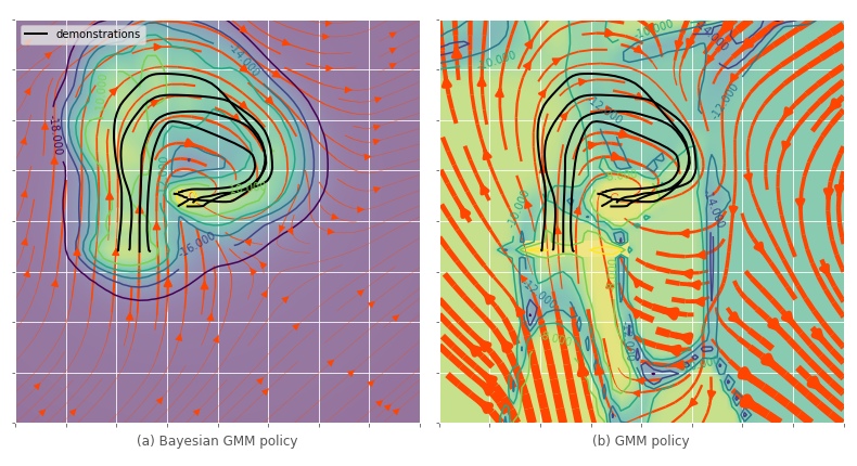
Figure 1: Comparison of Bayesian and non-Bayesian GMM conditional distributions. The flow field represents the expectation of $p(\bm{u}|\bm{x},\bm{X},\bm{U})$ and the colormap its entropy $\mathcal{H}(p(\bm{u}|\bm{x},\bm{X},\bm{U}))$. Yellow color is for lower entropy, meaning higher certainty. The black lines are the demonstrations $\bm{X}$ (a) Bayesian model: Certainty is localized in the vicinity of the demonstrations. The policy retrieved further away can result in poor generalization, but the system is aware of this through the uncertainty estimate. (b) Non-Bayesian model: The entropy only relates to the variations of the demonstrated policy instead of a Bayesian uncertainty.

II Related work

Several works have tackled the distributional shift problem in the general case. In [1], Ross et al. used a combination of expert and learner policy. In [5], perturbations are added in order to force the expert to demonstrate recovery strategies, resulting in a more robust policy.

More closely related to our manipulation tasks, Khansari-Zadeh et al. have used a similar approach to ours to learn a policy of the form $\bm{\dot{x}}=f(\bm{x})$ [3]. They used conditional distributions $p(\bm{\dot{x}}|\bm{x})$ in a joint model of $p(\bm{x},\bm{\dot{x}})$ represented as a Gaussian mixture model (GMM). A structure was imposed on the parameters to guarantee asymptotic convergence. As an alternative, we propose to exploit the uncertainty information of a Bayesian GMM, resulting in a less constrained approach that can scale easily to higher dimensions.

Dynamical movement primitives (DMP) is a popular approach that combines a stable controller (spring-damper system) with non-linear forcing terms decaying over time through the use of a phase variable, ensuring convergence at the end of the motion [6]. A similar approach is used in [2] where the non-linear part is encoded using conditional distributions in GMM. Due to their underlying time dependence, these approaches are often limited to either point-to-point or cyclic motions of known period, with limited temporal and spatial robustness to perturbations.

Another approach to avoid these problems is to model distributions of states or trajectories instead of policies [7, 4]. However, these techniques are limited to the imitation of trajectories and cannot handle easily misaligned or partial demonstrations of movements.

Inverse optimal control [8], which tries to find the objective minimized by the demonstrations, is another direction to increase robustness and generalization. It often requires more training data and is computationally heavy.

If a reward function for the task is accessible, an interesting alternative is to combine the proposed policy imitation strategy with reinforcement learning [9, 10], where the imitation loss can reduce the exploration phase while the reinforcement learning overcomes the limits of imitation.

III Bayesian Gaussian mixture model conditioning

Numerous regression techniques exist and have been applied to robotics. In this section, we derive a Bayesian version of Gaussian mixture conditioning [11], which was already used in [2, 3]. Besides uncertainty quantification, we start by listing the characteristics required in our tasks to motivate the need for a different approach.

Multimodal conditional

Policies from human demonstrations are never optimal but exhibit some stochasticity. In some tasks, for example implying obstacle avoidance, there could be multiple clearly separated paths. Fig. 2 illustrates this idea. Our approach should be able to encode arbitrarily complex conditional distributions. Existing approaches such as locally weighted projection regression (LWPR) [12] or Gaussian process regression (GPR) [13] only model unimodal conditional distribution. In its original form, GPR assumes homoscedasticity (constant covariance over the state).

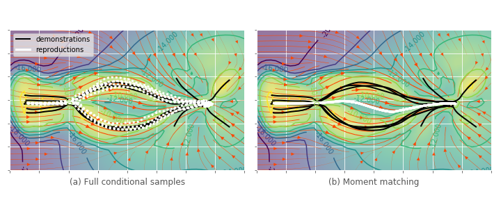
Figure 2: Advantages of encoding multimodal policy $p(\bm{u}|\bm{x})$. The demonstrations show how to reach a point while avoiding an obstacle. At a given position, the distribution of velocity is bimodal, indicating to go either upwards or downwards. (a) Multiple reproductions executed by sampling from an expressive multimodal policy $p(\bm{u}|\bm{x})$ as in (18). (b) Reproduction with a unimodal policy, where moment matching was applied to (18). The average command indicates to go straight, which results in a failure.

Efficient and robust computation

Most Bayesian models can be computationally demanding for both learning and prediction. For fast and interactive learning, we seek to keep a low training time (below 5 sec for the tasks shown in the experiments). For reactivity and stability, the prediction should be below 1 ms. We seek to avoid difficult model selection/hyperparameters tuning, for the approach to be applied in a wide range of tasks, controllers and robotic platforms.

Wide-ranging data

The approach should be able to encode very simple policies with a few datapoints and more complex ones when more datapoints are available.

Representing a joint distribution as a Gaussian mixture model and computing conditional distribution is simple and fast [11], with various applications in robotics [2, 3]. Bayesian regression methods approximate the posterior distribution $p(\bm{\theta}|\bm{X},\bm{Y})$ of the model parameters $\bm{\theta}$, given input $\bm{X}$ and output $\bm{Y}$ datasets. Then, predictions are made by marginalizing over the parameters posterior distribution, in order to propagate model uncertainties to predictions

$$p(\bm{y}|\bm{x},\bm{X},\bm{Y})=\int_{\bm{\theta}}p(\bm{y}|\bm{x},\bm{\theta})p(\bm{\theta}|\bm{X},\bm{Y})d\bm{\theta},$$ (1)

where $\bm{x}$ is a new query. This distribution is called posterior predictive. Parametric non-Bayesian methods typically rely on a single point estimate of the parameters $\bm{\theta}^{\star}$ such as maximum likelihood. A variety of methods, adapted to the various model, exists for approximating $p(\bm{\theta}|\bm{X},\bm{Y})$. For example, variational methods, Monte Carlo methods or expectation propagation. For its scalability and efficiency, we present here a variational method using conjugate priors and mean field approximation, see [14] for details.

III-A Bayesian analysis of multivariate normal distribution

We first focus on the Bayesian analysis of multivariate normal distribution (MVN), also detailed in [15], and then treat the mixture case. As a notation, we use $\bm{z}$ to denote $\begin{bmatrix}\bm{x}^{\scriptscriptstyle\top}\,\bm{y}^{\scriptscriptstyle\top}\end{bmatrix}^{\scriptscriptstyle\top}$, a joint observation of input and output. $\bm{Z}$ denotes the joint dataset.

Prior

The conjugate prior of the MVN is the normal-Wishart distribution. The convenience of a conjugate prior is the closed-form expression of the posterior. The normal-Wishart distribution is a distribution over mean $\bm{\mu}$ and precision matrix $\bm{\Lambda}$,

$$p(\bm{\mu},\bm{\Lambda}) =\mathcal{NW}(\bm{\mu},\bm{\Lambda}|\bm{\mu}_{0},\kappa,\nu,\bm{T}),$$ (2)

$$=\mathcal{N}\big{(}\bm{\mu}|\bm{\mu}_{0},(\kappa\bm{\Lambda})^{-1}\big{)}\mathcal{W}_{\nu}(\bm{\Lambda}|\bm{T}),$$ (3)

where $\bm{T}$ and $\nu$ are the scale matrix and the degree of freedom of the Wishart distribution, and $\kappa$ is the precision of the mean.

Posterior

The closed form expression for the posterior is

$$p(\bm{\mu},\bm{\Lambda}|\bm{X}) =\mathcal{N}\big{(}\bm{\mu}|\bm{\mu}_{n},(\kappa_{n}\bm{\Lambda}_{n})^{-1}\big{)}\mathcal{W}_{\nu_{n}}(\bm{\Lambda}_{n}|\bm{T}_{n}),$$ (4)

$$\bm{\mu}_{n} =\frac{\kappa\bm{\mu}_{0}+n\bar{\bm{z}}}{\kappa+n},$$ (5)

$$\bm{T}_{n} =\bm{T}+\bm{S}+\frac{\kappa n}{\kappa+n}(\bm{z}_{0}-\bar{\bm{z}})(\bm{\mu}_{0}-\bar{\bm{z}})^{\scriptscriptstyle\top},$$ (6)

$$\bm{S} =\sum_{i=1}^{n}(\bm{z}_{i}-\bar{\bm{z}})(\bm{z}_{i}-\bar{\bm{z}})^{\scriptscriptstyle\top},$$ (7)

$$\nu_{n} =\nu+n,\quad\kappa_{n}=\kappa+n,$$ (8)

where $n$ is the number of observations and $\bar{\bm{z}}$ is the empirical mean. As for conjugate priors, the prior distribution can be interpreted as pseudo-observations to which the dataset is added.

Posterior predictive

Computing the posterior predictive distribution

$$p(\bm{z}|\bm{Z})=\int_{\bm{\Lambda},\bm{\mu}}p(\bm{z}|\bm{\mu},\bm{\Lambda})p(\bm{\mu},\bm{\Lambda}|\bm{Z})d\bm{\Lambda}d\bm{\mu},$$ (9)

yields a multivariate t-distribution with degree of freedom $\nu_{n}-d+1$

$$p(\bm{z}|\bm{Z})=t_{\nu_{n}-d+1}\big{(}\bm{z}|\,\bm{\mu}_{n},\frac{\bm{T}_{n}(\kappa_{n}+1)}{\kappa_{n}(\nu_{n}-d+1)}\big{)},$$ (10)

where $d$ is the dimensionality of $\bm{z}$. The multivariate t-distribution has heavier tails than the MVN. The MVN is a special case of this latter, when the degree of freedom parameter tends to infinity, which corresponds to having infinitely many observations.

Conditional posterior predictive

For our application, we are interested in computing conditional distributions in the joint distribution of our input $\bm{x}$ and output $\bm{y}$. We rewrite the result from (9) as

$$p(\bm{x},\bm{y}\,|\bm{X},\bm{Y})=t_{\nu_{\bm{z}}}(\bm{\mu}_{\bm{z}},\bm{\Sigma}_{\bm{z}}).$$ (11)

Following [16], the multivariate t-distribution conditional distribution is also a multivariate t-distribution,

$$p(\bm{y}\,|\bm{x},\bm{X},\bm{Y})=t_{\nu_{\bm{y}|\bm{x}}}(\bm{\mu}_{\bm{y}|\bm{x}},\bm{\Sigma}_{\bm{y}|\bm{x}}),$$ (12)

with

$$\nu_{\bm{y}|\bm{x}} =\nu_{\bm{x}\bm{y}}+d_{\bm{x}},$$ (13)

$$\bm{\mu}_{\bm{y}|\bm{x}} =\bm{\mu}_{\bm{y}}+\bm{\Sigma}_{\bm{y}\bm{x}}\bm{\Sigma}_{\bm{x}}^{-1}(\bm{x}-\bm{\mu}_{\bm{x}}),$$ (14)

$$\bm{\Sigma}_{\bm{y}|\bm{x}} =\frac{\nu_{\bm{x}\bm{y}}\!+\!(\bm{x}\!-\!\bm{\mu}_{\bm{x}})^{\scriptscriptstyle\top}\bm{\Sigma}_{\bm{x}}^{-1}(\bm{x}\!-\!\bm{\mu}_{\bm{x}})}{\nu_{\bm{x}\bm{y}}+d_{\bm{x}}}(\bm{\Sigma}_{\bm{y}}\!-\!\bm{\Sigma}_{\bm{y}\bm{x}}\bm{\Sigma}_{\bm{x}}^{-1}\bm{\Sigma}_{\bm{y}\bm{x}}^{\scriptscriptstyle\top}),$$ (15)

where $d_{\bm{x}}$ is the dimension of $\bm{x}$, with $\bm{\mu}_{\bm{z}}$ and $\bm{\Sigma}_{\bm{z}}$ decomposed as

$$\bm{\mu}_{\bm{z}}=\begin{bmatrix}\bm{\mu}_{\bm{x}}\\ \bm{\mu}_{\bm{y}}\\ \end{bmatrix},\quad\bm{\Sigma}_{\bm{z}}=\begin{bmatrix}\bm{\Sigma}_{\bm{x}}&\bm{\Sigma}_{\bm{x}\bm{y}}\\ \bm{\Sigma}_{\bm{y}\bm{x}}&\bm{\Sigma}_{\bm{y}}\\ \end{bmatrix}.$$ (16)

The mean $\bm{\mu}_{\bm{y}|\bm{x}}$ follows a linear trend on $\bm{x}$ and the scale matrix $\bm{\Sigma}_{\bm{y}|\bm{x}}$ increases as the query point is far from the input marginal distribution, with a dependence on the degree of freedom. These expressions are similar to MVN conditional but the scale ($\bm{\Sigma}_{\bm{y}\bm{x}}=\bm{\Sigma}_{\bm{x}}-\bm{\Sigma}_{\bm{y}\bm{x}}\bm{\Sigma}_{\bm{x}}^{-1}\bm{\Sigma}_{\bm{y}\bm{x}}^{\scriptscriptstyle\top}$ for the MVN) has an additional factor, increasing uncertainty as $\bm{x}$ is far from the known distribution.

III-B Bayesian analysis of the mixture model

Using the conjugate prior for the MVN leads to very efficient training of mixtures with mean-field approximation or Gibbs sampling. Efficient algorithms similar to expectation maximization (EM) can be derived. For brevity, we will here only summarize the results relevant to our application (see e.g., [14] for details). Using mean-field approximation and variational inference, the posterior predictive distribution of a mixture of MVN is a mixture of multivariate t-distributions

$$p(\bm{z}|\bm{Z})=\sum_{k=1}^{K}\pi_{k}\ t_{\nu_{k}-d+1}(\bm{z}|\,\bm{\mu}_{k},\frac{\bm{T}_{k}(\kappa_{k}+1)}{\kappa_{k}(\nu_{k}-d+1)}).$$ (17)

The conditional posterior distribution is then also a mixture

$$p(\bm{y}|\,\bm{x},\bm{X},\bm{Y}) =\sum_{k=1}^{K}p(k|\,\bm{x},\bm{X},\bm{Y})p(\bm{y}|\,k,\bm{x},\bm{X},\bm{Y}),$$ (18)

where we need to compute the marginal probability of the component $k$ given the input $\bm{x}$

$$p(k|\,\bm{x},\bm{X}) =\frac{\pi_{k}t_{\nu_{\bm{x},k}}(\bm{x}|\,\bm{\mu}_{\bm{x},k},\bm{\Sigma}_{\bm{x},k})}{\sum_{j}\pi_{j}t_{\nu_{\bm{x},j}}(\bm{x}|\,\bm{\mu}_{\bm{x},j},\bm{\Sigma}_{\bm{x},j})}$$ (19)

and apply conditioning in each component using (13)–(15)

$$p(\bm{y}|k,\bm{x},\bm{X},\bm{Y}) =t_{\nu_{\bm{x}|\bm{y},k}}(\bm{y}|\,\bm{\mu}_{\bm{y}|\bm{x},k},\bm{\Sigma}_{\bm{y}|\bm{x},k}).$$ (20)

Equation (19) exploits the property that marginals of multivariate-t distributions are of the same family [16].

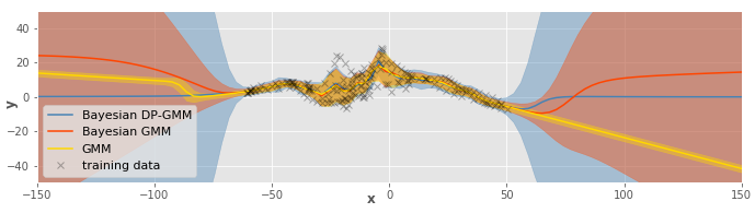
Figure 3: Conditional distribution $p(\bm{y}|\bm{x})$ where $p(\bm{x},\bm{y})$ is modeled as a mixture of Gaussians. The mean and the standard deviation are represented by applying moment matching on the multimodal conditional distribution. (blue) The joint distribution has a Dirichlet process prior. (red) The prior is a Dirichlet distribution, with a fixed number of clusters. (yellow) The prediction is done without integrating the posterior distribution, which results in a lack of estimation of its uncertainty far from training data.

Dirichlet distribution or Dirichlet process

In [14], the Bayesian Gaussian mixture model is presented with a Dirichlet distribution prior over the mixing coefficients $\bm{\pi}$. An alternative is to use a Dirichlet process, a non-parametric prior with an infinite number of clusters. For the learning part, this allows the model to cope with an increasing number of datapoints and adapting the model complexity. Very efficient online learning strategies [17] exist. With a Dirichlet process, the posterior predictive distribution is similar to (17) but with an additional mixture component being the prior predictive distribution of the MVN. Conditional distribution given points far from the training data would have the shape of the marginal predictive prior, similarly as in GPR. Fig. 3 illustrates the difference, when conditioning, between the Dirichlet process and the distribution. When applied to a policy, it means that when diverging from the distribution of visited states, the control command distribution will match the given prior.

With a Dirichlet process, the model presented here is a particular case of [18], having the advantages of faster training with variational techniques and faster retrieval with closed-form integration.

When using a Dirichlet process prior, the number of clusters is determined by the data. This number is particularly influenced by the hyperparameters $\nu$ and $\bm{T}$ of the Wishart prior. A high $\nu$ leads to a high number of small clusters. On the contrary, a high $\bm{T}$ implies an important regularization on the covariances, which leads to a small number of big clusters. In some cases, it is easier to determine a fixed number of clusters with a Dirichlet distribution. In that case, $\nu$ and $\bm{T}$ can be set small, such that the posterior is more influenced by the data than by the prior.

IV Product of policy distributions

In cognitive science, it is known that two heads are better than one if they can provide an evaluation of their uncertainty when bringing their knowledge together [19]. In machine learning, fusing multiples sources is referred to as products of experts (PoE) [20]. In this section, we propose to exploit the uncertainty presented in the above, by fusing multiple policies $p_{1}(\bm{u}|\bm{x}),\dots,p_{M}(\bm{u}|\bm{x})$, coming from multiple sources or learning strategies.

In the general case, computing the mode of a PoE requires optimization, which is inappropriate in applications where the policy should be computed fast. However, when assuming an MVN for each expert $i$, $\mathcal{N}_{i}(\bm{x}|\,\bm{\mu}_{i},\bm{\Lambda}^{-1}_{i})$, the computation becomes lightweight. The product distribution has the closed form expression

$$\bar{\bm{\Lambda}}=\sum_{i=1}^{M}\bm{\Lambda}_{i},\quad\bar{\bm{\mu}}=\bar{\bm{\Lambda}}^{-1}\sum_{i=1}^{M}\bm{\Lambda}_{i}\bm{\mu}_{i},$$ (21)

where $\bm{\Lambda}$ denotes the precision matrix (inverse of covariance). This result has an intuitive interpretation: the estimate is an average of the sources weighted by their precisions.

If we want to fuse the policy imitation that we proposed in (18) with another policy, several alternatives are possible. If speed is a priority, for example when using torque control, the full conditional distribution (18) could be approximated as an MVN, which enables fast fusion using (21). For this purpose, moment matching can be used. This approximation can be harmful in case of clearly multimodal policies, as illustrated in Fig. 2(b). If more time is available for computation and/or a higher precision is required, (18) can be estimated as a mixture of MVN by applying moment matching to each cluster. The product of a mixture of MVN and another mixture (or just an MVN) is also a mixture of MVN [21]. To give an idea about computation time, the product between two mixtures of $K=25$ components and $d_{u}=7$ dimensionality of $\bm{u}$ takes about 3 ms on a standard computer with NumPy. The product between this mixture and an MVN takes about 0.25 ms. In the experiments presented in Sec. V, the global moment matching approximation with an MVN is used, as the tasks do not exhibit multimodality.

IV-A Examples of controllers

We present a set of policies that can be combined to increase robustness and that will be used in the experiments.

Optimal control

If the task can be formulated as a cost (e.g., attaining a given state), an interesting strategy is to use optimal control (OC). Classically, these techniques require an accurate model of the system and are subject to local minima (for example, in an environment with obstacles). In combination with imitation, we propose to use OC with crude model approximations (e.g., without modeling obstacles).

In order to combine the policy, we need the OC solver to retrieve a distribution of commands $p(\bm{u})$. A first way will be to use the solution as the mean of an MVN and fix its precision heuristically, such that it dominates the imitation policy outside of the training data. A more rigorous way is to use the maximum entropy principle [22], retrieving a near optimal stochastic policy. However, this technique is much more computationally demanding than the standard OC problem. When using linear dynamics and quadratic cost, the maximum entropy solution can be retrieved very efficiently [23], using linear quadratic tracking (LQT) [24] as

$$p(\bm{u}_{t}|\bm{x}_{t})=\mathcal{N}(-\bm{K}_{t}\bm{x}_{t}+\bm{c}_{t},\bm{Q}_{t}^{-1}).$$ (22)

Time-dependent policy

For discrete point-to-point tasks, it is possible to use a policy that will ensure convergence at the end of the motion. This structure is already given in dynamical movement primitives (DMP) [6] or in [2], where a phase variable is used to switch between controllers. Our approach allows for a more complex and better-motivated fusion of policies. This stable controller can either be engineered or computed with OC. Here, we used an LQT where the cost on the state is active only at the end of the task. The controller, in the form of (22), has gain $\bm{K}_{t}$ and precision matrix $\bm{Q}_{t}$ increasing along time, as shown in Fig. 4b for starting and final time.

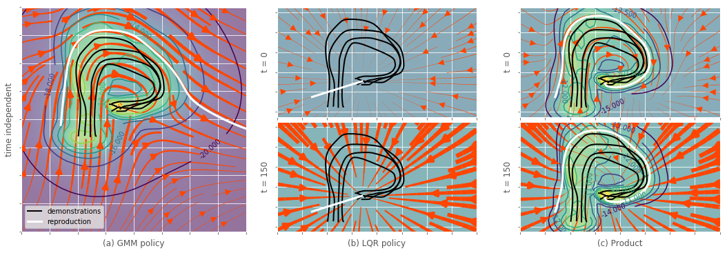
Figure 4: Mixing imitation and LQT, with the final target specified. (a) Bayesian GMM policy: Time-independent policy learned with the presented method. (b) LQT policy: Only final state target distribution is specified, which results in a time-dependent policy whose control gains increases along time. The shown policies are for $t\in[0,150]$. (c) Combination: The combination is a time-dependent policy. It applies, at the beginning, the imitation policy in zones of high certainty, and is lightly converging outside. At the end of the task, it becomes more strongly converging all over the states.

Conservative policy

We also propose to use a policy that brings us back to the distribution of states where the policy is known, as in [25]. In their case, the policy was designed as a PD controller, but we propose to use OC or model-based policy search for more generality. In the proposed GMM, the conservative policy can either be optimized to minimize the uncertainty of the imitation policy (e.g., given by the entropy of the conditional distribution) or to converge to the marginal distribution of states. For the experiments, we chose to solve the latter with an LQT. A local quadratic approximation of $-\log p(\bm{x}|\bm{X})$ from (17) is used as cost on the state. A quadratic cost on the control $\bm{u}$ is set to limit forces or velocities. For an increased precision, this policy can also be learned using maximum entropy model-based policy search [26].

Fig. 5b illustrates this policy and shows that this technique can encode cyclic motions, which would have been difficult to achieve with the previous propositions. We also note that the combination given by (21) is more complex than the scalar combination proposed in [25] because it can take into account that policies may have variable precisions along different axes.

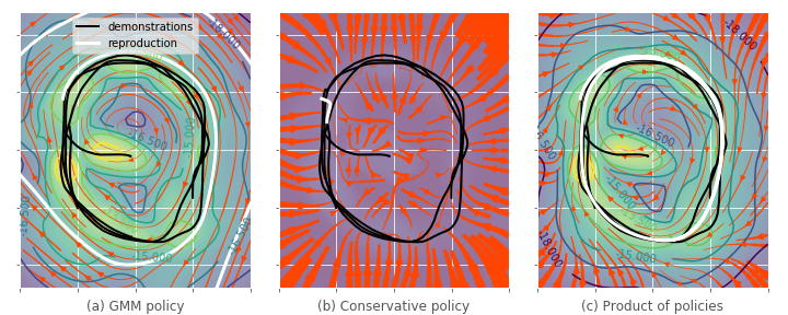
Figure 5: Encoding a limit cycle can be done without any modification of our approach. (a) Bayesian GMM policy: By only applying this policy, the robot quickly diverges from the cycle and goes into regions where the policy is unknown. (b) Conservative policy: This policy forces the robot to go back to regions where the robot knows the policy, which has a stabilizing function. (c) Product of policies: The product of the two policies follows the imitated policy in known regions and converges back to these regions when the robot is brought outside.

Accompanying Python codes and videos are available at https://gitlab.idiap.ch/rli/pbdlib-python.

V Experiments

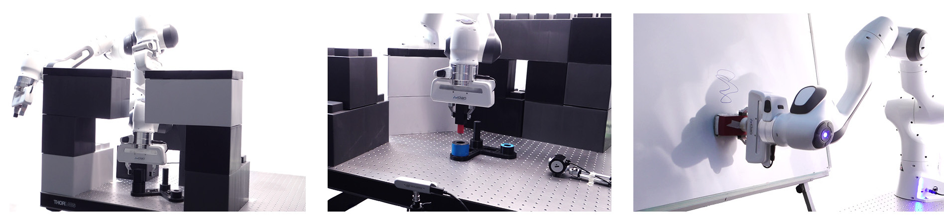
Figure 6: (left) Obstacle navigation with joint velocity controller. (center) Vision-based peg-in-hole with velocity controlled robot. (right) White board wiping with force controlled robot.

Three experiments are presented to demonstrate that the proposed approach can be used in a variety of tasks. They are performed on a 7-axis Panda (Franka Emika) robot.

V-A Obstacle navigation

In the first experiment, the robot should navigate through fixed obstacles from various initial configurations in order to grasp an object, see Fig. 6-(left). The system is defined with joint angles $\bm{x}=\bm{q}$ as states and joint velocities $\bm{u}=\bm{\dot{q}}$ as control commands.

In total, 13 demonstrations were recorded (totaling 115 sec of recording). Eight demonstrations were recorded by starting far from the desired point, showing how to avoid the obstacles. The five others were only local, providing more precise demonstrations at the end of the motion, where an accurate alignment between the gripper and the object to grasp is required.

We chose to fuse the imitation policy with a LQT conservative policy, converging to the marginal distribution of joint angles. This conservative policy is similar to the one illustrated in Fig. 5 for a 2D system. The non-Bayesian policy, as planned, was quickly diverging and dangerously accelerating outside of the demonstrated regions of the state space.

While an optimal control/planning approach would require the modeling of the obstacles and the robot volume, ours was able to propose a solution robust to a wide range of starting points, that could be set up intuitively within only a few minutes. This experiment also illustrates the advantages of learning a distribution of policies instead of trajectories as in [4]. The teaching time can be optimized with partial demonstrations. Moreover, there is no need for an additional mechanism to realign the demonstrations in time.

V-B Vision-based peg-in-hole

In the second task, the robot should insert a peg in a moving hole by looking from two cameras placed on the side, see Fig. 6-(center). The center of the red peg and the center of the blue tube (top part) are extracted by image processing. The diameter of the peg is 15% smaller than the hole, such that the task can be solved with an imperfect vision system and without impedance control. The state is the pixel displacement from the hole and the peg from the two cameras $\bm{x}=\begin{bmatrix}\bm{p}_{1}^{\scriptscriptstyle\top},\bm{p}_{2}^{\scriptscriptstyle\top}\end{bmatrix}^{\scriptscriptstyle\top}$. The control command is the Cartesian velocity of the gripper in robot frame (the orientation was held fixed) $\bm{u}=\bm{v}^{\mathrm{ee}}$, but joint angle velocities would have been possible as well, likely requiring some additional demonstrations.

As an evaluation, the robot was initialized at 10 random postures (with the peg still being seen by the two cameras). We evaluated its capacity to insert the peg without touching the border of the hole or hitting the support (receptacle). Multiple combinations of policies were used (among imitation, conservative and optimal control, as presented in Sec. IV). The conservative policy was an LQR, similar to the one in the previous experiment. Instead of converging to the distribution of known joint angles, this policy acts in pixel space.

Computing this policy requires the dynamic model $\bm{x}_{t+1}=f(\bm{x}_{t},\bm{u}_{t})$, unknown in this experiment. It is learned by recording 10 sec of random motions. The relation between the position of the end-effector $\bm{x}^{\mathrm{ee}}$ and the pixel position of camera $i$, $\bm{p}_{i}=g_{i}(\bm{x}^{\mathrm{ee}})$, is learned using the method presented in Sec. III. The Jacobian of $g_{i}$, which links $\bm{v}^{\mathrm{ee}}$ to pixel velocities, is then used to build a linearized version of $f(\bm{x}_{t},\bm{u}_{t})$. Due to observation noise, this approach is more robust than directly learning $f(\bm{x}_{t},\bm{u}_{t})$.

The cost for the optimal control policy is defined as the negative log-likelihood of the distribution of desired final states, encoded as an MVN. The cost on the state is only active at the end of the LQT planning horizon, corresponding to the length of the longest demonstration. This allows variability during the task and forces convergence at the end of the task. The cost on $\bm{u}$ is the negative log-likelihood of the distribution of control command $\bm{u}$ during the demonstrations. Results are reported in Table I.

TABLE I: Results of the peg-in-hole task with different combinations of policies (imitation, optimal control (OC) and conservative (CS)). The task is considered a success if the peg is in the hole without touching the border, or with a slight touch that did not displace the receptacle. Hitting the border or being stuck is considered as a failure.

Policies	success rate	(10 trials)	failure
	without touching	with touching
Imitation only	0.3	0.1	0.6
Im. + OC	0.4	0.4	0.2
Im. + CS	0.7	0.1	0.2
Im. + CS + OC	0.8	0.1	0.1
OC	0.0	0.1	0.9

Imitation alone shows the effect of an accumulation of errors. It often fails if brought far from the known regions of the state space. It also only slowly stops. Since the obstacles are neither modeled nor learned, the OC policy results in a straight line motion to the target (as illustrated in Fig. 4b) and thus almost always hits the obstacles or the border of the receptacle. It only works when employed very close to the goal. It provides good correction in this context when used in combination with the other policies. The conservative policy has a relevant effect to converge back to the known regions of the state space and provide a good improvement of the results.

In this experiment, we are in a similar situation to [3], where we control the velocity of an object. But as the relation between end-effector and pixel velocities is not known beforehand and might change, the approach in [3] is not applicable.

V-C Force based board wiping

In the third task, we demonstrate learning of a force policy within a cyclic motion. The robot has to wipe a board by applying a force against it while doing circular motions. The state is composed of the position and linear velocity of the end-effector (defined at the gripper) in the robot base frame $\bm{x}\!=\!\begin{bmatrix}{\bm{x}^{\mathrm{ee}}}^{\scriptscriptstyle\top},{\bm{v}^{\mathrm{ee}}}^{\scriptscriptstyle\top}\end{bmatrix}^{\scriptscriptstyle\top}$. The control command is the force to apply at the end-effector $\bm{u}\!=\!\bm{F}^{\mathrm{ee}}$, which is then transformed to torques with $\bm{\tau}={\bm{J}(\bm{q})}^{\scriptscriptstyle\top}\bm{F}^{\mathrm{ee}}+\bm{c}(\bm{q},\bm{\dot{q}})+\bm{g}(\bm{q})$, where Coriolis $\bm{c}$ and gravity $\bm{g}$ compensation torques are added. To be able to record forces during demonstrations, bilateral teleoperation is used with a second 7-axis Panda robot. The two end-effectors are linked to each other using a virtual spring-damper system with a position offset. One demonstration of the circular cyclic motion is performed, 7 others are performed showing how to start/recover when not in contact with the board or outside of the wiping area. As in the first experiment, we used a combination of the imitation policy and the conservative policy, which forces convergence to the marginal distribution of position and velocity. By executing only the imitation policy, the robot is pressing against the board, applying a very imprecise force tangentially to the wiping path to compensate for friction. It diverges quickly from the original path. The applied forces are quite clumsy (except perpendicularly to the board) and show a wide variance, which explains the failure of this policy. The conservative policy alone executes circle-shaped motions very robustly without applying any force against the board, resulting in no cleaning, as shown in Fig. 7.

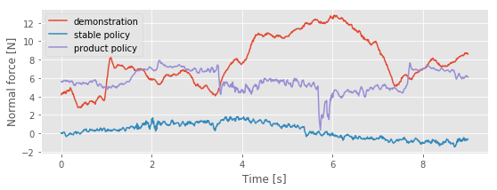
Figure 7: Comparison of normal forces applied by the robot on the board. Using the conservative (or stable) policy results in almost no force. Using the product of policies, the forces are much closer to the recorded ones.

Fusion with full precision matrices as in (21) allows the imitation policy to be used perpendicularly to the board while using the conservative policy along the other directions, in accordance to their respective precisions. The resulting policy is very robust, even when the user strongly perturbs the robot, showing that it slowly converges back to the board and to the circular motion before starting wiping. This robustness and combination of periodic (wiping) and discrete (converging back to the wiping area) would have been very difficult to achieve (if not impossible) with trajectory-based or time-dependent approaches.

VI Conclusion

In this paper, we presented a Bayesian regression technique with several interesting characteristics for robotic applications. We applied this technique to the common problem of distributional shift in policy imitation, where the uncertainty can be exploited for an intelligent fusion of controllers. Many approaches for learning robotic manipulation tasks impose structure or restrictions on the policy, which limit their range of applications. We showed in three distinct experiments that our approach can be applied without modification to many state-control systems and to a variety of tasks (discrete or/and periodic).

Finally, we believe that this method is well suited in an active learning scenario, which would be investigated in future work. In such a case, the robot would ask for demonstrations in unknown regions in order to optimize the learning process. The efficiency of training and the closed-form predictive distribution of the proposed method makes it possible to maximize complex learning criteria.

References

- [1] S. Ross, G. Gordon, and D. Bagnell, “A reduction of imitation learning and structured prediction to no-regret online learning,” in Proc. Intl Conf. on Artificial Intelligence and Statistics (AISTATS), 2011, pp. 627–635.
- [2] M. Hersch, F. Guenter, S. Calinon, and A. Billard, “Dynamical system modulation for robot learning via kinesthetic demonstrations,” IEEE Trans. on Robotics, vol. 24, no. 6, pp. 1463–1467, 2008.
- [3] S. M. Khansari-Zadeh and A. Billard, “Learning stable nonlinear dynamical systems with gaussian mixture models,” IEEE Trans. on Robotics, vol. 27, no. 5, pp. 943–957, 2011.
- [4] A. Paraschos, C. Daniel, J. R. Peters, and G. Neumann, “Probabilistic movement primitives,” in Advances in Neural Information Processing Systems (NIPS), 2013, pp. 2616–2624.
- [5] M. Laskey, J. Lee, R. Fox, A. D. Dragan, and K. Y. Goldberg, “DART: Noise injection for robust imitation learning,” in Conference on Robot Learning (CoRL), 2017, pp. 143–156.
- [6] S. Schaal, J. Peters, J. Nakanishi, and A. Ijspeert, “Learning movement primitives,” in Intl Journal of Robotic Research. Springer, 2005, pp. 561–572.
- [7] S. Calinon, D. Bruno, and D. G. Caldwell, “A task-parameterized probabilistic model with minimal intervention control,” in Proc. IEEE Intl Conf. on Robotics and Automation (ICRA), 2014, pp. 3339–3344.
- [8] C. Finn, S. Levine, and P. Abbeel, “Guided cost learning: Deep inverse optimal control via policy optimization,” in Proc. Intl Conf. on Machine Learning (ICML), 2016, pp. 49–58.
- [9] A. Rajeswaran, V. Kumar, A. Gupta, G. Vezzani, J. Schulman, E. Todorov, and S. Levine, “Learning complex dexterous manipulation with deep reinforcement learning and demonstrations,” Proc. Robotics: Science and Systems (RSS), 2018.
- [10] A. Nair, B. McGrew, M. Andrychowicz, W. Zaremba, and P. Abbeel, “Overcoming exploration in reinforcement learning with demonstrations,” in Proc. IEEE Intl Conf. on Robotics and Automation (ICRA). IEEE, 2018, pp. 6292–6299.
- [11] H. G. Sung, “Gaussian mixture regression and classification,” PhD thesis, Rice University, Houston, Texas, 2004.
- [12] S. Schaal, C. G. Atkeson, and S. Vijayakumar, “Scalable techniques from nonparametric statistics for real time robot learning,” Applied Intelligence, vol. 17, no. 1, pp. 49–60, 2002.
- [13] C. E. Rasmussen, “Gaussian processes in machine learning,” in Advanced lectures on machine learning. Springer, 2004, pp. 63–71.
- [14] C. M. Bishop, Pattern Recognition and Machine Learning (Information Science and Statistics). Secaucus, NJ, USA: Springer, 2006.
- [15] K. P. Murphy, “Conjugate Bayesian analysis of the Gaussian distribution,” University of British Columbia, Tech. Rep., 2007.
- [16] M. Roth, On the multivariate t distribution. Linköping University Electronic Press, 2013.
- [17] M. C. Hughes and E. Sudderth, “Memoized online variational inference for dirichlet process mixture models,” in Advances in Neural Information Processing Systems (NIPS), 2013, pp. 1133–1141.
- [18] L. A. Hannah, D. M. Blei, and W. B. Powell, “Dirichlet process mixtures of generalized linear models,” Journal of Machine Learning Research, vol. 12, no. Jun, pp. 1923–1953, 2011.
- [19] B. Bahrami, K. Olsen, P. E. Latham, A. Roepstorff, G. Rees, and C. D. Frith, “Optimally interacting minds,” Science, vol. 329, no. 5995, pp. 1081–1085, 2010.
- [20] G. E. Hinton, “Products of experts,” Proc. Intl Conf. on Artificial Neural Networks (ICANN), pp. 1–6, 1999.
- [21] M. J. F. Gales and S. S. Airey, “Product of Gaussians for speech recognition,” Computer Speech and Language, vol. 20, no. 1, pp. 22–40, jan 2006.
- [22] B. D. Ziebart, A. L. Maas, J. A. Bagnell, and A. K. Dey, “Maximum entropy inverse reinforcement learning.” in Proc. AAAI Conference on Artificial Intelligence, vol. 8. Chicago, IL, USA, 2008, pp. 1433–1438.
- [23] S. Levine and P. Abbeel, “Learning neural network policies with guided policy search under unknown dynamics,” in Advances in Neural Information Processing Systems (NIPS), 2014, pp. 1071–1079.
- [24] M. Bohner and N. Wintz, “The linear quadratic tracker on time scales,” International Journal of Dynamical Systems and Differential Equations, vol. 3, no. 4, pp. 423–447, 2011.
- [25] A. Paraschos, E. Rueckert, J. Peters, and G. Neumann, “Model-free probabilistic movement primitives for physical interaction,” in Proc. IEEE/RSJ Intl Conf. on Intelligent Robots and Systems (IROS). IEEE, 2015, pp. 2860–2866.
- [26] S. Levine, “Reinforcement learning and control as probabilistic inference: Tutorial and review,” arXiv preprint arXiv:1805.00909, 2018.