Self-consistent band calculation of slab phase in neutron-star crust

Abstract

Fully self-consistent band calculation has been performed for slab phase in neutron-star inner crust, using the BCPM energy density functional. Optimized slab structure is calculated at given baryon density either with the fixed proton ratio or with the beta-equilibrium condition. Numerical results indicate the band gap of in order of keV to tens of keV, and the mobility of dripped neutrons are enhanced by the Bragg scattering, which leads to the macroscopic effective mass, $\bar{m}^{*}_{z}/m_{n}=0.65\sim 0.75$ near the bottom of the inner crust in neutron stars. We also compare the results of the band calculation with those of the Thomas-Fermi approximation. The Thomas-Fermi approximation becomes invalid at low density with high proton ratio.

I Introduction

Compact stars, such as white dwarfs and neutron stars, provide extreme phases of matters. In cold white dwarfs, the materials are ionized by high pressure, producing the degenerate Fermi gas of electrons and crystalized ions. In vicinity of the surface of neutron stars, called outer crust, similar structure are expected to exist. A little deeper in the neutron stars with greater density, namely at inner crust, neutrons also form a degenerate Fermi gas. We expect that the neutrons are in the ${}^{1}S_{0}$ pair condensation phase, showing superfluidity. There, neutron-rich nuclei form a Coulomb crystal which coexist with gas of superfluid neutrons and electrons. Even deeper in the stars, before the neutron-rich nuclei are dissolved to form uniform nuclear matter (“core”), we expect exotic phases of nuclear matter, called nuclear pasta Ravenhall et al. (1983); Hashimoto et al. (1984); Oyamatsu (1993).

In the pasta phase, the competition between the repulsive Coulomb and the attractive nuclear interactions rearrange the nuclei into exotic non-spherical shapes. These shapes are often called name of pasta, such as spaghetti (rod shape) and lasagna (slab shape). These phases of non-spherical nuclei were first predicted using a simple liquid drop model Ravenhall et al. (1983); Hashimoto et al. (1984). The Thomas-Fermi approximation to a simplified Skyrme-like energy density functional confirmed the stability of these phases Oyamatsu (1993). Since the pasta phase has a regular structure analogous to the crystal, quantum mechanically, it should be treated as a system with a periodic potential, namely, with the Bloch boundary condition. Chamel has performed the band calculation to predict large effective mass $m^{*}$ of neutrons due to the Bragg scattering by the periodic potential produced by the crystalline structure Chamel (2012). The calculation predicts that the ratio $m^{*}/m_{n}$, where $m_{n}$ is the bare neutron mass, can be 10 or even larger.

The structure of the inner crust has a significant influence on observed properties of neutron stars. Especially, the entrainment effect could have a significant consequence on an interpretation of glitch phenomena. The pulsar glitches first were observed in 1969 at the Vela pulsar Radhakrishnan and Manchester (1969); Reichley and Downs (1969), in which the spin rate of the pulsar suddenly increases. Since then, we have observed more than 100 pulsars showing the glitch phenomena. The current consensus view is that the vortices in the superfluid neutron gas in the inner crust are responsible for the glitches Anderson and Itoh (1975). The spin-rate difference between the superfluid neutrons and the rest of the star is accumulated until the glitch occurs. If the superfluid neutrons in the inner crust are a reservoir of the angular momentum, in order to explain the magnitude of glitches, the ratio between the neutrons’ and the total moments of inertia should be $I_{n}/I\sim 1-1.5$ % Link et al. (1999). These values are consistent with typical nuclear matter equations of state (EOS). However, taking into account the entrainment effect, the required ratio $I_{n}/I$ is multiplied by $m^{*}/m_{n}$, which leads to serious difficulties to regard the superfluid neutrons as the angular momentum reservoir Andersson et al. (2012).

The structure of the inner crust also influences the electrical and the thermal conductivity. A high electrical resistive layer in the bottom part of the inner crust, supposed to be the pasta layers, could lead to magnetic field decay of neutron stars. This limits the maximum spin period, which is consistent with lack of observation of isolated X-ray pulsars with spin period longer than 12 s Pons et al. (2013). Since the thermal conductivity is likely related to the electrical one, the effect of the nuclear pasta may be also seen in the late time crust cooling Horowitz et al. (2015).

The calculation by Chamel Chamel (2012) predicted that the density of conduction neutrons $n^{c}_{n}$ is significantly smaller than the density of unbound neutrons $n^{f}_{n}$, leading to the large effective mass, $m^{*}/m_{n}=n_{n}^{f}/n_{n}^{c}$. This may require us to revise our interpretation of pulsar glitches. However, the calculation of Ref. Chamel (2012) is not self-consistent. He adopted a periodic one-body potential based on the extended Thomas-Fermi calculation in the Wigner-Seitz cell. In this paper, we perform the band calculation using a modern energy density functional in a fully self-consistent manner. As the first step toward the systematic calculation of various phases, we treat the slab phase, neglecting spin-orbit and pairing correlations.

The paper is organized as follows. In Sec. II, we give the formulation of the self-consistent calculation of slab nuclei with dripped neutrons using the band theory. We perform numerical calculations for systems with a given proton ratio and at the beta-equilibrium condition. The entrainment effect is measured by effective mass. In Sec. III, we show results of the numerical calculations. For comparison, we also perform calculation with the Thomas-Fermi approximation which has been frequently used in the past. Summary and future perspectives are given in Sec. IV.

II Band theory for slab phase

The inner crust of neutron stars have been studied quantum mechanically with the Wigner-Seitz approximation, in which the periodic structure is decomposed into independent spherical cells of a cell radius $R_{\rm cell}$. Unbound neutrons are treated with different boundary conditions at $R_{\rm cell}$ according to the parity of the orbitals Negele and Vautherin (1973). The Wigner-Seitz approximation is relatively well justified for the outer crust, while it is questionable for the inner crust Baldo et al. (2006). Especially, the entrainment effect cannot be taken into account in this approximation.

II.1 Reduction to one dimension

The proper treatment of unbound neutrons in a crystallized nuclear matter requires the band theory of solids Ashcroft and Mermin (1976). Although the band theory is a well-known established theory, as far as we know, its application to neutron-star crust was first performed by Chamel in 2005 Chamel (2005). The essential difference from the treatment of an isolated nucleus is the boundary condition for the single-particle (Kohn-Sham) wave functions. They satisfy the Bloch boundary condition Ashcroft and Mermin (1976):

$$\varphi_{\alpha,\bm{k}}^{(q)}(\bm{r}+\bm{T},s)=\exp(i\bm{k}\cdot\bm{T})\varphi_{\alpha,\bm{k}}^{(q)}(\bm{r},s),$$ (1)

where $\bm{k}$ is the Bloch wave vector and $\alpha$ is the band index. The vector $\bm{T}$ is a lattice translational vector. The spin and isospin indices are denoted by $s=\pm 1/2$ and $q=(n,p)$. We focus the present work on the slab phase, and choose the normal direction to the slab nuclei as the $z$ direction. See Fig. 1. The system is assumed to be uniform along the tangential ($x$-$y$) directions, and the spin-orbit potential is neglected for simplicity. Assuming the distance $a$ between neighboring slab nuclei, the lattice vector becomes $\bm{T}=T_{x}\bm{e}_{x}+T_{y}\bm{e}_{y}+na\bm{e}_{z}$, where $T_{x}$ and $T_{y}$ are arbitrary real numbers, $n$ is an arbitrary integer number, and $\bm{e}_{j}$ is a unit vector along $j=(x,y,z)$ direction. The wave functions become separable, in which those with respect to $x$ and $y$ coordinates are the plane waves. Thus, we may write the wave function $\varphi_{\alpha,\bm{k}}^{(q)}(\bm{r})$ of Eq. (1) in a form

$$\varphi_{\alpha,\bm{k}}^{(q)}(\bm{r})=\exp(ik_{x}x+ik_{y}y)\cdot e^{ik_{z}z}\phi_{\alpha,\bm{k}}^{(q)}(z)=e^{i\bm{k}\cdot\bm{r}}\phi_{\alpha,\bm{k}}^{(q)}(z),$$ (2)

where the wave functions $\phi_{\alpha,\bm{k}}^{(q)}(z)$ satisfy the periodic boundary condition

$$\phi_{\alpha,\bm{k}}^{(q)}(z+a)=\phi_{\alpha,\bm{k}}^{(q)}(z).$$ (3)

Hereafter, we omit the index $s$, because the wave functions are spin-independent. Thus, the model space can be reduced into the one-dimensional unit cell, $0\leq z<a$. Here, $\bm{k}=k_{x}\bm{e}_{x}+k_{y}\bm{e}_{y}+k_{z}\bm{e}_{z}$, and $(k_{x},k_{y})$ represents the nucleon momentum in the tangential ($x$-$y$) directions, while $k_{z}$ corresponds to the Bloch wave number which can be restricted inside the first Brillouin zone, $-\pi/a<k_{z}\leq\pi/a$.

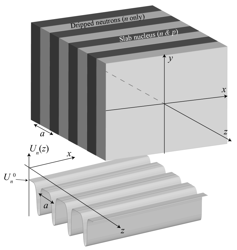
Figure 1: (Top) Schematic picture of the slab phase. The slabs are parallel to the $x$-$y$ plane. (Bottom) Schematic illustration of potential for neutrons $U_{n}(z)$ in the $z$-$x$ plane.

The wave functions are determined by the self-consistent (Kohn-Sham) equations,

$$h_{q}[\rho]\varphi_{\alpha,\bm{k}}^{(q)}(\bm{r})=\epsilon_{\alpha,\bm{k}}^{(q)}\varphi_{\alpha,\bm{k}}^{(q)}(\bm{r}),$$ (4)

with the single-particle Hamiltonian

$$h_{q}[\rho]=-\nabla\cdot\frac{1}{2m_{q}^{*}(\bm{r})}\nabla+U_{q}(\bm{r}).$$ (5)

In this paper, we adopt the unit of $\hbar=1$. In the present case, since the slab is assumed to be uniform in the the effective mass $m_{q}^{*}(\bm{r})$ and the selfconsistent potential $U_{q}(\bm{r})$ depends only on $z$. It should be noted that the effective mass $m_{q}^{*}(\bm{r})$ here is different from those discussed in Secs. II.4 and III. When we need to distinguish different effective masses in the present paper, we call $m_{q}^{*}(\bm{r})$ microscopic effective mass, and those in Sec. II.4 macroscopic ones. The wave functions of Eq. (2) lead to

$$\left(\frac{k_{\rho}^{2}}{2m_{q}^{*}(z)}+h_{k_{z}}^{(q)}\right)\phi_{\alpha,\bm{k}}^{(q)}(z)=\epsilon_{\alpha,\bm{k}}^{(q)}\phi_{\alpha,\bm{k}}^{(q)}(z),$$ (6)

with $k_{\rho}^{2}\equiv k_{x}^{2}+k_{y}^{2}$ and

$$h_{k_{z}}^{(q)}\equiv\left(-i\partial_{z}+k_{z}\right)\frac{1}{2m_{q}^{*}(z)}\left(-i\partial_{z}+k_{z}\right)+U_{q}(z).$$ (7)

We end up at the one-dimensional equation (6), though the wave functions still depend on $(k_{x},k_{y})$ through the $z$-dependent kinetic energy term. If the effective mass $m_{q}^{*}(z)$ is identical to the bare nucleon mass $m_{q}$, the single-particle wave functions $\phi_{\alpha,\bm{k}}^{(q)}(z)$ become independent from $(k_{x},k_{y})$; $\phi_{\alpha,\bm{k}}^{(q)}\rightarrow\phi_{\alpha,k_{z}}^{(q)}$. Since this significantly reduces computational task, in this study, we adopt an energy density functional with no derivative terms (Sec. II.2). Equation (6) is reduced to

$$h_{k_{z}}^{(q)}\phi_{\alpha,k_{z}}^{(q)}(z)=e_{\alpha,k_{z}}^{(q)}\phi_{\alpha,k_{z}}^{(q)}(z),$$ (8)

where $e_{\alpha,k_{z}}^{(q)}$ represent the energy band as functions of $k_{z}$. The single-particle energy is given by

$$\epsilon_{\alpha,\bm{k}}^{(q)}=\frac{k_{\rho}^{2}}{2m_{q}}+e_{\alpha,k_{z}}^{(q)}.$$ (9)

The states with $\epsilon_{\alpha,\bm{k}}^{(q)}<\mu_{q}$ are occupied, where $\mu_{q}$ is the Fermi energy (chemical potential).

In practice, the Bloch wave number, $-\pi/a<k_{z}\leq\pi/a$ is discretized into $N_{k}$ points. The calculation with $N_{k}$ points of $k_{z}$ is identical to the calculation with the periodic boundary condition in a space $N_{k}$ times larger than the unit cell. The wave functions are normalized as

$$\int_{0}^{a}\left|\phi_{\alpha,k_{z}}^{(q)}(z)\right|^{2}dz=\frac{1}{N_{k}}.$$ (10)

The density is calculated as

$$\rho_{q}(z) = 2\sum_{\alpha,k_{z}}\left|\phi_{\alpha,k_{z}}^{(q)}(z)\right|^{2}\int\frac{dk_{x}dk_{y}}{(2\pi)^{2}}\theta(\mu_{q}-\epsilon_{\alpha,\bm{k}}^{(q)})$$ (11)

$$= \frac{m_{q}}{\pi}\sum_{\alpha,k_{z}}^{\rm occ}\left|\phi_{\alpha,k_{z}}^{(q)}(z)\right|^{2}\left(\mu_{q}-e_{\alpha,k_{z}}^{(q)}\right),$$

where $\theta(x)$ is a step function and $\sum^{\rm occ}$ means the summation with respect to occupied (hole) orbitals only. The summation with respect to $k_{z}$ is taken over $N_{k}$ discretized values of $k_{z}$. The baryon (nucleon) number density is defined as $\rho_{B}(z)\equiv\rho_{n}(z)+\rho_{p}(z)$. In a similar manner, the kinetic density is given by

$$\tau_{q}(z) \equiv 2\sum_{\alpha,k_{z}}\int\frac{dk_{x}dk_{y}}{(2\pi)^{2}}\left|\nabla\varphi_{\alpha,\bm{k}}^{(q)}(\bm{r})\right|^{2}\theta(\mu_{q}-\epsilon_{\alpha,\bm{k}}^{(q)})$$ (12)

$$= \frac{m_{q}^{2}}{\pi}\sum_{\alpha,k_{z}}^{\rm occ}\left(\mu_{q}-e_{\alpha,k_{z}}^{(q)}\right)^{2}\left|\phi_{\alpha,k_{z}}^{(q)}(z)\right|^{2}$$

$$+ \frac{m_{q}}{\pi}\sum_{\alpha,k_{z}}^{\rm occ}\left(\mu_{q}-e_{\alpha,k_{z}}^{(q)}\right)\left|\left(ik_{z}+\frac{d}{dz}\right)\phi_{\alpha,k_{z}}^{(q)}\right|^{2}.$$

II.2 Nuclear and electronic energy density functionals

The average baryon number density $n_{B}$ is given by $n_{B}=n_{n}+n_{p}$, with the average neutron and proton densities,

$$n_{q}\equiv\frac{1}{a}\int_{0}^{a}\rho_{q}(z)dz.$$ (13)

The proton fraction $Y_{p}$ is defined by $Y_{p}\equiv n_{p}/n_{B}$. In this study, the electrons are assumed to be uniform. The charge neutrality requires that the electron density is equal to the average proton density, $n_{e}=n_{p}$. The charge density is simply given by $\rho_{c}(\bm{r})\equiv\rho_{p}(\bm{r})-n_{e}$, neglecting the charge form factor of protons. The electrons are treated as degenerated relativistic Fermi gas with the Fermi momentum, $p_{F}$. The Fermi energy is given as $\epsilon_{F}^{(e)}=\sqrt{m_{e}^{2}c^{4}+p_{F}^{2}c^{2}}=m_{e}c^{2}\cosh\theta_{F}$, where $\theta_{F}$ is determined by the electron density, $3\pi^{2}n_{e}=(m_{e}c\sinh\theta_{F})^{3}$. Their energy divided by the baryon (nucleon) number $A$ is given as $E_{e}/A=K_{e}/A+E_{C}^{(e)}/A$ with

$$\frac{K_{e}}{A} = \frac{4\pi}{n_{B}}\int_{0}^{p_{F}}\frac{p^{2}dp}{(2\pi)^{3}}\sqrt{m_{e}^{2}c^{4}+p^{2}c^{2}}$$ (14)

$$= \frac{m_{e}^{4}c^{5}}{32\pi^{2}n_{B}}\left(\sinh 4\theta_{F}-4\theta_{F}\right),$$

$$\frac{E_{C}^{(e)}}{A} = -\frac{3e^{2}n_{e}^{4/3}}{4n_{B}}\left(\frac{3}{\pi}\right)^{1/3},$$ (15)

where we use the Slater approximation for the exchange energy. The direct term of the Coulomb energy $-(2an_{B})^{-1}\int_{0}^{a}V_{C}(z)n_{e}dz$, vanishes, because of the charge neutrality condition for the Coulomb potential;

$$\int_{0}^{a}V_{C}(z)dz=0.$$ (16)

The Coulomb potential for protons $V_{C}$ ($-V_{C}$ for electrons) is calculated by solving the Poisson equation

$$\frac{d^{2}}{dz^{2}}V_{C}(z)=-4\pi e^{2}\rho_{c}(z),$$ (17)

with the condition (16).

For nuclear part, we adopt the energy density functional (EDF) of BCPM Baldo et al. (2013), neglecting the spin-orbit coupling terms. This EDF is constructed so as to reproduce properties of both the nuclear matter, predicted by the Brueckner-Hartree-Fock calculation, and experimental data of finite nuclei. Another practical reason of this choice is that the kinetic density $\tau_{q}(\bm{r})$ is present only in the kinetic energy terms. Thus, we can use Eq. (8) instead of Eq. (6), which significantly reduces the computational cost.

In the BCPM functional, the nuclear energy is written as

$$E_{B}=\sum_{q=n,p}K_{q}+E_{\rm vol}+E_{\rm sur}+E_{\rm C}^{(p)}.$$ (18)

Here, $K_{q}$ is the kinetic energy of neutrons ($q=n$) and protons ($q=p$). The potential energy is divided into two parts, the “volume” (bulk) and “surface” parts. The volume part $E_{\rm vol}$ reproduces the nuclear matter properties, and the surface part $E_{\rm sur}$ is added to reproduce observed properties of finite nuclei Baldo et al. (2013). The kinetic energy per baryon is given by

$$\frac{K_{q}}{A}=\frac{1}{an_{B}}\int_{0}^{a}\frac{\tau_{n}(z)+\tau_{p}(z)}{2m_{q}}dz.$$ (19)

The volume part is given as

$$\frac{E_{\rm vol}}{A} = \frac{1}{an_{B}}\int_{0}^{a}\left[P_{s}(\rho_{B}(z))\left\{1-\beta^{2}(z)\right\}\right.$$ (20)

$$\quad\quad\quad\quad\left.+P_{n}(\rho_{B}(z))\beta^{2}(z)\right]\rho_{B}(z)dz,$$

where $\beta(z)\equiv(\rho_{n}(z)-\rho_{p}(z))/\rho_{B}(z)$. The functionals $P_{s}(\rho_{B})$ and $P_{n}(\rho_{B})$ are given in polynomial with respect to $\rho_{B}(z)$ Baldo et al. (2013). The surface part is

$$\frac{E_{\rm sur}}{A} = \frac{\pi r_{0}^{2}}{2an_{B}}\sum_{q,q^{\prime}}V_{qq^{\prime}}\left[\int_{0}^{a}dz\int_{0}^{a}dz^{\prime}\rho_{q}(z)e^{-\frac{(z-z^{\prime})^{2}}{r_{0}^{2}}}\rho_{q^{\prime}}(z^{\prime})\right.$$ (21)

$$\quad\quad\quad\quad\quad\quad\left.-g\int_{0}^{a}dz\rho_{q}(z)\rho_{q^{\prime}}(z)\right].$$

This expression ignores the interaction with nucleons outside of the unit cell. In order to take into account interactions with nucleons in the neighboring cells, we replace the gaussian $e^{-(z-z^{\prime})^{2}/r_{0}^{2}}$ in Eq. (21) by

$$v(z)\equiv e^{-(z-z^{\prime})^{2}/r_{0}^{2}}+e^{-(z-z^{\prime}-a)^{2}/r_{0}^{2}}+e^{-(z-z^{\prime}+a)^{2}/r_{0}^{2}}.$$ (22)

This treatment is well justified at $a\gg r_{0}$. The parameter $g$ is given, in this approximation, by $g\equiv\int_{0}^{a}v(z)dz$. See Ref. Baldo et al. (2013) for values of the parameters $V_{qq^{\prime}}$ and $r_{0}$.

The Coulomb energy per baryon is given by

$$\frac{E_{C}^{(p)}}{A} = \frac{1}{2an_{B}}\int_{0}^{a}V_{C}(z)\rho_{p}(z)dz$$ (23)

$$\quad-\frac{3e^{2}}{4an_{B}}\left(\frac{3}{\pi}\right)^{1/3}\int_{0}^{a}\rho_{p}^{4/3}(z)dz.$$

The direct part of the total Coulomb energy is

$$\left(E_{C}^{(e)}+E_{C}^{(p)}\right)_{D}=\frac{e^{2}}{2}\iiint d^{3}\bm{r}\iiint d^{3}\bm{r}^{\prime}\frac{\rho_{c}(z)\rho_{c}(z^{\prime})}{\left|\bm{r}-\bm{r}^{\prime}\right|}.$$ (24)

II.3 Self-consistent solutions

The potentials $U_{q}(z)$ is given by the variation of the interaction energy with respect to the density.

$$U_{q}(z)=\frac{\delta(E_{\rm vol}+E_{\rm sur}+E^{(q)}_{C})}{\delta\rho_{q}(z)},$$ (25)

where $E^{(n)}_{C}=0$. Apparently, these potentials are functionals of $\rho_{q}(z)$, and the self-consistency is required for solutions of Eq. (8). In the present case, since we have the effective mass of $m_{q}^{*}(z)=m_{q}$ the single-particle Hamiltonian of Eq. (7) is

$$h_{k_{z}}^{(q)}=\frac{1}{2m_{q}}\left(-i\partial_{z}+k_{z}\right)^{2}+U_{q}(z).$$ (26)

In the band calculation of solid, the Hamiltonian of electrons explicitly depends on the coordinates of ions ($\bm{R}$) and the structure optimization is performed using the Feynman-Hellman theorem, $d\langle H\rangle/d\bm{R}=\langle dH/d\bm{R}\rangle=0$. However, for the band calculation of neutron-star crust, the Hamiltonian is independent from nuclear configuration. The crystalline structure is defined “by hand” in the beginning, in order to reduce the large-space calculation into that of a unit cell. Thus, the use of the Feynman-Hellman theorem is not trivial. In the present paper, we perform the optimization with respect to the lattice constant (slab interval) $a$, by explicitly calculating different values of $a$.

The total energy of the system is simply given by the sum of nuclear and electronic energies, $E_{B}+E_{e}$. We perform calculations with a given value of the average proton density $n_{p}$. Thus, the uniform electron density $n_{e}=n_{p}$ is also fixed. In order to find the optimum value of the lattice constant $a$, we should minimize the total energy,

$$\left.\frac{\partial(E_{B}+E_{e})}{\partial a}\right|_{n_{p}}=\left.\frac{\partial E_{B}}{\partial a}\right|_{n_{p}}=0.$$ (27)

Therefore, the minimization of the nuclear energy gives the optimal value of $a$.

II.3.1 Fixed proton ratio

In an event of supernova, during collapse of a giant star, the nuclear matter at a large variety of density and proton ratio is supposed to appear. When we fix the average neutron and proton densities, the electron energy, $E_{e}=K_{e}+E_{C}^{(e)}$ of Eqs. (14) and (15), plays any role neither for solutions of the self-consistency equation (8), nor for the optimization of the slab distance $a$. Thus, we solve Eq. (8) with $n_{e}=n_{p}$ for a given value of the lattice constant $a$.

The iterative calculation at a given $a$ is performed according to the following procedure.

1. Input the initial density, $\rho_{q}^{(i)}(z)$ ($i=0$), and calculate the energy per baryon $E_{B}^{(i)}/A$.

2. Calculate the potential $U_{q}(z)$.

3. Solve Eq. (8) to determine the wave functions $\phi_{\alpha,k_{z}}^{(q)}(z)$ and the band energy $e_{\alpha,k_{z}}^{(q)}$.

4. Determine the chemical potential $\mu_{q}$ so as to obtain the target density $n_{q}$.

5. Calculate the new densities, $\rho_{q}(z)$ and $\tau_{q}(z)$, according to Eqs. (11) and (12), respectively.

6. Calculate the nuclear energy $E_{B}/A$. Check the convergence condition, $|(E_{B}-E_{B}^{(i)})/E_{B}|<\eta$. If this is not satisfied, update the density; $\rho_{q}^{(i+1)}(z)=(1-\omega)\rho_{q}^{(i)}(z)+\omega\rho_{q}(z)$, set $E_{B}^{(i+1)}=E_{B}$, and go back to Step 2.

Here, we adopt the parameters, $\eta=10^{-10}$ and $\omega=0.1$.

II.3.2 Beta equilibrium

The electron energy is completely irrelevant for the self-consistent solutions in the case that both $n_{p}$ and $n_{n}$ are fixed. In contrast, it affects the condition of beta equilibrium. The beta-equilibrium condition is given by

$$(\mu_{p}+m_{p}c^{2})+\mu_{e}=(\mu_{n}+m_{n}c^{2}).$$ (28)

Note that the electron chemical potential contains its rest mass,

$$\mu_{e}=\frac{1}{V}\frac{\partial E_{e}}{\partial n_{e}}=\sqrt{m_{e}^{2}c^{4}+p_{F}^{2}c^{2}}-e^{2}\left(\frac{3n_{e}}{\pi}\right)^{1/3}.$$ (29)

We perform the calculation at a given average density of protons, $n_{p}$. Since the charge neutral condition requires $n_{e}=n_{p}$, the condition (28) determines the neutron chemical potential. Then, the iterative procedure (Steps $1\sim 6$) is exactly the same as the previous one in Sec. II.3.1, except for Step 4 where $\mu_{n}$ is given by the condition $\mu_{n}=\mu_{p}+\mu_{e}-(m_{n}-m_{p})c^{2}$.

II.4 Entrainment and effective mass

In the outer crust, both neutrons and protons are bound in nuclei. In the rest frame of crust, even with a perturbative force on neutrons, there would be no current. In contrast, the inner crust has conduction neutrons which are dripped from the nuclear binding. Thus, the band filling property determines whether they are “conductor” or “insulator”. We expect that the slab phase of the inner crust is always a conductor, because the neutron single-particle energy $\epsilon_{\alpha,\bm{k}}^{(n)}$ in Eq. (9) is continuous and has no gap. Nevertheless, its $z$ component, $e_{\alpha,k_{z}}^{(n)}$, represents the band structure and has band gaps at $k_{z}=\pm\pi/a$, which may affect the conduction properties along the $z$ direction (normal to the slabs).

The group velocity of neutrons in the band $\epsilon_{\alpha,\bm{k}}^{(n)}$ is given by Ashcroft and Mermin (1976)

$$\bm{v}^{(n)}_{\alpha,\bm{k}}=\nabla_{\bm{k}}\epsilon^{(n)}_{\alpha,\bm{k}}.$$ (30)

Assuming no interband transition between bands with different $\alpha$, the acceleration under a force $\bm{F}$ on neutrons is given by

$$\frac{d\bm{v}^{(n)}_{\alpha,\bm{k}}}{dt}=\left(\frac{d\bm{k}}{dt}\cdot\nabla_{\bm{k}}\right)\bm{v}_{\alpha,\bm{k}}^{(n)}=\left(\bm{F}\cdot\nabla_{\bm{k}}\right)\nabla_{\bm{k}}\epsilon^{(n)}_{\alpha,\bm{k}},$$ (31)

where we used the acceleration theorem, $d\bm{k}/dt=\bm{F}$ Callaway (1976); Ashcroft and Mermin (1976). Writing the $i$-th component ($i=x,y,z$) of $\bm{v}$ as

$$\frac{dv^{i}}{dt}=\sum_{j}\left(\frac{1}{m^{*}}\right)_{\alpha,\bm{k}}^{ij}F_{j},$$ (32)

we obtain the macroscopic effective mass tensor

$$\left(\frac{1}{m^{*}}\right)^{ij}_{\alpha,\bm{k}}\equiv\frac{\partial^{2}\epsilon^{(n)}_{\alpha,\bm{k}}}{\partial k_{i}\partial k_{j}}.$$ (33)

In the present case, the effective mass is diagonal ($(1/m^{*})^{ij}=\delta^{ij}/m_{i}^{*}$), and for $i=x,y$, they are equal to the bare neutron mass, $m^{*}_{i}=m_{n}$.

The neutron mobility can be measured by Eq. (33) summed over the occupied orbits.

$$\mathcal{K}^{ij}\equiv 2\sum_{\alpha}\int\frac{d^{3}k}{(2\pi)^{3}}\frac{\partial^{2}\epsilon_{\alpha,\bm{k}}^{(n)}}{\partial k_{i}\partial k_{j}}\theta(\mu_{n}-\epsilon_{\alpha,\bm{k}}^{(n)}).$$ (34)

For the present case of the slab phase, it is transformed to

$$\mathcal{K}^{ij}\equiv\frac{2}{aN_{k}}\sum_{\alpha,k_{z}}\int\frac{dk_{x}dk_{y}}{(2\pi)^{2}}\frac{\partial^{2}\epsilon_{\alpha,\bm{k}}^{(n)}}{\partial k_{i}\partial k_{j}}\theta(\mu_{n}-\epsilon_{\alpha,\bm{k}}^{(n)}),$$ (35)

and $\mathcal{K}^{ij}$ is diagonal in the Cartesian coordinates $(x,y,z)$, namely, $\mathcal{K}^{ij}=0$ for $i\neq j$. The mobility coefficients for $x$ and $y$ directions are simply given as $\mathcal{K}^{xx}=\mathcal{K}^{yy}=n_{n}/m_{n}$, The $z$ component is calculated as

$$\mathcal{K}^{zz}\equiv\frac{m_{n}}{\pi aN_{k}}\sum_{\alpha,k_{z}}^{\rm occ}\frac{d^{2}e_{\alpha,k_{z}}^{(n)}}{dk_{z}^{2}}\left(\mu_{n}-e_{\alpha,k_{z}}^{(n)}\right),$$ (36)

and equivalently given by

$$\mathcal{K}^{zz}\equiv\frac{m_{n}}{\pi aN_{k}}\sum_{\alpha,k_{z}}^{\rm occ}\left(\frac{de_{\alpha,k_{z}}^{(n)}}{dk_{z}}\right)^{2}$$ (37)

From this mobility coefficient, we may define conduction neutron density $n_{i}^{c}$ which are supposed to freely move in the neutron-star crust along the $i$ direction ($i=x,y,z$) Chamel (2012).

$$n_{i}^{c}\equiv m_{n}\mathcal{K}^{ii}.$$ (38)

Trivially, we have $n_{x}^{c}=n_{y}^{c}=n_{n}$, which means that all the neutrons in the slab phase are effectively free in the $x$-$y$ plane. In contrast, the $z$ component of the conduction neutron density $n_{z}^{c}$ may be hindered, not only by the bound neutrons inside the slab, but also by the Bragg scattering due to the periodic nuclear potential. The latter is called entrainment effect Carter et al. (2005, 2006); Chamel (2012).

The reduction of $n_{z}^{c}$ from the neutron density $n_{n}$ is quantified as an effective mass Carter et al. (2006):

$$m_{z}^{*}\equiv\frac{n_{n}}{\mathcal{K}^{zz}}=m_{n}\frac{n_{n}}{n_{z}^{c}},$$ (39)

With this definition (39), the effective mass diverges in the outer crust where there are no dripped neutrons.

Another definition is given as the ratio to “free” neutrons. In this paper, we adopt two kinds of definition. The first one is given by neutrons whose single-particle energy is larger than the maximum value of the neutron potential $U_{n}^{0}\equiv\max(U_{n}(z))$ (See also Fig. 1). With this definition, we have $n_{n}^{f}=0$ for $\mu_{n}<U_{n}^{0}$, which corresponds to the slab nuclei without the dripped neutrons. For $\mu_{n}\geq U_{n}^{0}$,

$$\tilde{n}_{n}^{f} \equiv \frac{2}{aN_{k}}\sum_{\alpha,k_{z}}\int\frac{dk_{x}dk_{y}}{(2\pi)^{2}}\theta(\mu_{n}-\epsilon_{\alpha,\bm{k}}^{(n)})\theta(\epsilon_{\alpha,\bm{k}}^{(n)}-U_{n}^{0})$$ (40)

$$= n_{n}-\frac{m_{n}}{\pi aN_{k}}\sum_{e_{\alpha,k_{z}}^{(n)}<U_{n}^{0}}\left(U_{n}^{0}-e_{\alpha,k_{z}}^{(n)}\right).$$

The free neutrons of Eq. (40) includes those with $\epsilon_{\alpha,\bm{k}}^{(n)}>U_{n}^{0}>e_{\alpha,k_{z}}^{(n)}$. Since the Kohn-Sham Hamiltonian in the present case is separable in each direction of $x$, $y$, and $z$, the neutrons with $e_{\alpha,k_{z}}^{(n)}<U_{n}^{0}$ are practically bound in the $z$ direction. In this sense, it may be reasonable to define the “free” neutrons in the $z$ direction as those with $e_{\alpha,k_{z}}^{(n)}>U_{n}^{0}$.

$$\bar{n}_{n}^{f} \equiv \frac{2}{aN_{k}}\sum_{\alpha,k_{z}}\int\frac{dk_{x}dk_{y}}{(2\pi)^{2}}\theta(\mu_{n}-\epsilon_{\alpha,\bm{k}}^{(n)})\theta(e_{\alpha,k_{z}}^{(n)}-U_{n}^{0})$$ (41)

$$= n_{n}-\frac{m_{n}}{\pi aN_{k}}\sum_{e_{\alpha,k_{z}}^{(n)}<U_{n}^{0}}\left(\mu_{n}-e_{\alpha,k_{z}}^{(n)}\right).$$

Following these two definitions of “free” neutrons, Eqs. (40) and (41), we denote two kinds of effective mass as

$$\tilde{m}_{z}^{*}\equiv\frac{\tilde{n}_{n}^{f}}{\mathcal{K}^{zz}}=m_{n}\frac{\tilde{n}_{n}^{f}}{n_{z}^{c}},\quad\quad\bar{m}_{z}^{*}\equiv\frac{\bar{n}_{n}^{f}}{\mathcal{K}^{zz}}=m_{n}\frac{\bar{n}_{n}^{f}}{n_{z}^{c}},$$ (42)

It is obvious that $n_{n}\geq\tilde{n}_{n}^{f}\geq\bar{n}_{n}^{f}$, which leads to $m_{z}^{*}\geq\tilde{m}_{z}^{*}\geq\bar{m}_{z}^{*}$.

III Numerical results

The single-particle Hamiltonian in Eq. (26) has a property, $h_{k_{z}}^{(q)*}=h_{-k_{z}}^{(q)}$. Therefore, the solutions of Eq. (8) for negative $k_{z}$ can be constructed from those of positive $k_{z}$ as $\phi_{-k_{z}}^{(q)}=\phi_{k_{z}}^{(q)*}$ with $e_{\alpha,-k_{z}}^{(q)}=e_{\alpha,k_{z}}^{(q)}$. The first Brillouin zone can be further reduced to $0\leq k_{z}\leq\pi/a$ for the present calculation. When we solve Eq. (8) for discretized $k_{z}$ values of

$$k_{z}=\frac{\pi}{a}\frac{l}{N_{k}^{\prime}},\quad l=0,\cdots,N_{k}^{\prime},$$ (43)

the solutions for $k_{z}=-\frac{\pi}{a}\frac{l}{N_{k}^{\prime}}$ with $l=1,\cdots,N_{k}^{\prime}-1$ are also obtained ($N_{k}^{\prime}>0$). The number of $k_{z}$ points is $N_{k}=2N_{k}^{\prime}$. The calculation only with $k_{z}=0$ corresponds to $N_{k}=1$.

The $z$ coordinate in the unit cell ($0\leq z\leq a$) is discretized in a mesh of $\Delta z=0.2$ fm, and the nine-point finite-difference formula is used for differentiation in Eq. (8). The number of iteration, shown in Sec. II.3, necessary to reach the self-consistent solutions varies case by case; a few tens to thousands of iteration. Roughly speaking, more iterations are needed for calculations of the slab phase at lower density.

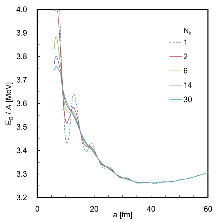
Figure 2: (Color online) Energy per nucleon $E_{B}/A$ as a function of lattice constant $a$, for the case of proton fraction $Y_{p}=0.05$ and baryon density $n_{B}=0.04$ fm^-1. The blue solid line shows the one obtained with the band calculation adopting $30$ points of the Bloch wave number, while the blue dashed line indicates that of periodic boundary condition. Those obtained with different $N_{k}$ are shown by solid lines with different colors.

III.1 Convergence with respect to number of $k$ points

First, we demonstrate that the periodic boundary condition, which were often adopted in mean-field calculations for finite nuclei, might lead to a wrong answer for the inner crust of neutron stars. The simple periodic condition at the end of the unit cell, $\varphi^{(q)}_{\alpha,\bm{k}}(x,y,z+a)=\varphi^{(q)}_{\alpha,\bm{k}}(x,y,z)$, corresponds to the band calculation with $k_{z}=0$ only ($N_{k}=1$). In Fig. 2, we show variation of energy with respect to the lattice constant $a$ for the case of proton fraction $Y_{p}=0.05$ and density $n_{B}=0.04$ fm^-1. The result obtained with the periodic boundary condition shows a strong oscillating pattern. The optimum value of $a$ is given by either $a=35.8$ fm or $41.4$ fm.

The calculation with periodic boundary condition may approximately provide a proper answer for the outer crust. However, for the inner crust, because of the presence of the dripped neutrons at the boundary, the energy shows a spurious oscillation as a function of $a$. Since the calculation with $N_{k}$ $k_{z}$-points corresponds to the one in a space of $0\leq z\leq N_{k}a$ with the periodic boundary condition, this simple exercise indicates necessity of large-space calculation for the inner crust.

This oscillation completely disappears for $a>10$ fm, when we take into account enough number of points for the Bloch wave number $k_{z}$. In Fig. 2, we also show results with different number of $N_{k}$. Beyond $N_{k}=10$, we hardly see difference in the scale of Fig. 2 for $a>10$ fm. The converged result for the optimum value of the lattice constant is $a=39.2$ fm. In the present study, we adopt $N_{k}=30$ which is enough to reach the convergence. Although $N_{k}=30$ may not be sufficient for a small lattice constant $a<10$ fm, we have confirmed that the obtained optimum values of $a$ are significantly larger than 10 fm.

III.2 Thomas-Fermi calculation for slab phase

In order to compare our result of the self-consistent band-theory calculation with the one of the Thomas-Fermi (TF) theory, we also perform the TF calculation. Since the interaction energy of the BCPM functional is given as a functional of $\rho_{q}(z)$, we adopt exactly the same form in the TF calculation. The kinetic density of Eq. (19) is replaced by

$$\tau_{q}\left[\rho\right]=\frac{3}{5}\left(3\pi^{2}\right)^{2/3}\rho_{q}^{5/3}(z)+\frac{\lambda_{W}}{\rho_{q}(z)}\left(\frac{d\rho_{q}}{dz}\right)^{2},$$ (44)

where $\lambda_{W}$ is a parameter of the Weizsäcker term given as $\lambda_{W}=1/36$ Ring and Schuck (1980).

For practical solutions, we use the imaginary-time method similar to Ref. Levit (1984). Introducing the auxiliary functions $u_{q}(z)$ to represent the density as $\rho_{q}(z)=u_{q}^{2}(z)$, the time evolution is given by

$$\left.u_{q}(z)\right|_{t+\delta t}=u_{q}(z)-\delta t\left(h_{q}[\rho]-\mu_{q}\right)u_{q}(z),$$ (45)

where $u_{q}(z)$ and $\rho_{q}(z)$ in the right hand side are functions at imaginary time $t$. Here, the “Hamiltonian” $h_{q}[\rho]$ is given by

$$h_{q}\left[\rho\right]\equiv\frac{-1}{2m_{q}}4\lambda_{W}\frac{d^{2}}{dz^{2}}+U_{q}(z)+\frac{1}{2m_{q}}\left\{3\pi^{2}\rho_{q}(z)\right\}^{2/3}.$$ (46)

The “chemical potentials” $\mu_{q}$ are chosen to keep the average density $n_{q}$ invariant for calculation with fixed $(n_{B},Y_{p})$.

$$\mu_{q}=\frac{1}{an_{q}}\int_{0}^{a}u_{q}(z)h_{q}[\rho]u_{q}(z)dz.$$ (47)

Although $\mu_{q}$ conserves the average density in the first order in $\delta t$, $u_{q}(z)$ are normalized every time to reproduce the given average density $n_{q}$. For calculation of beta equilibrium, $\mu_{q}$ are chosen to keep $n_{B}$ invariant, which leads to

$$\mu_{q} = \frac{1}{n_{B}}\Bigg{[}\frac{1}{a}\sum_{q^{\prime}=n,p}\int_{0}^{a}u_{q^{\prime}}(z)h_{q^{\prime}}u_{q^{\prime}}(z)dz$$ (48)

$$+n_{\bar{q}}\left\{\left(m_{\bar{q}}-m_{q}\right)c^{2}+(-1)^{\delta_{qp}}\mu_{e}\right\}\Bigg{]},$$

where $\bar{q}=n(p)$ for $q=p(n)$.

In practice, we adopt the imaginary-time step, $\delta t=2^{-8}$ MeV^-1 for calculation with fixed $(n_{B},Y_{p})$, and $\delta t=2^{-10}$ MeV^-1 for calculation of beta equilibrium. The $z$ coordinate in the unit cell ($0\leq z\leq a$) is discretized in a mesh of $\Delta z=0.2$ fm, and the nine-point finite-difference formula is used for differentiation in the imaginary-time evolution of Eq. (45) The convergence condition is given by

$$\frac{1}{n_{B}}\sum_{q}\int_{0}^{a}\left\{(h_{q}-\mu_{q})u_{q}(z)\right\}^{2}dz<10^{-12}\textrm{ MeV}^{2}.$$ (49)

Since the TF theory directly treats the density instead of wave functions, we may use the periodic boundary condition, $\rho_{q}(z)=\rho_{q}(z+a)$ which is equivalent to $u_{q}(z)=u_{q}(z+a)$ for the real auxiliary function.

The last term in Eq. (44) is called the Weizsäcker correction term, which takes into account the inhomogeneity and has no contribution to the uniform matter. The original value of $\lambda_{W}$, given by Weizsäcker, was $1/4$ instead of $1/36$ Weizsäcker (1935). The factor $\lambda_{W}=1/36$ is consistent with the gradient expansion and equivalently with the $\hbar$ expansion Ring and Schuck (1980). The importance of this Weizsäcker term will be demonstrated in Sec. III.3.

III.3 Comparison between band and TF calculations

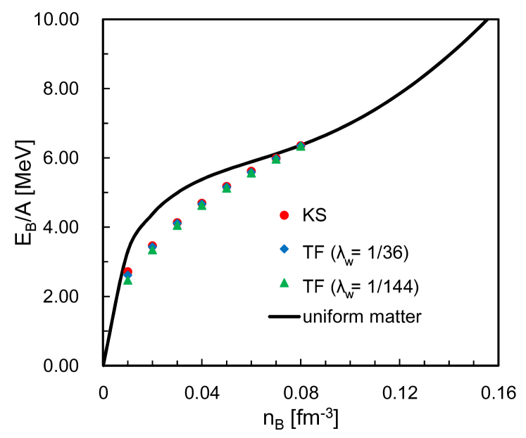
Figure 3: (Color online) Calculated nuclear energy per nucleon $E_{B}/A$ at beta equilibrium as a function of baryon density $n_{B}$. The results of TF approximation are shown by blue diamonds ($\lambda_{W}=1/36$) and green triangles ($\lambda_{W}=1/144$), while those of the band calculation are by red circles. The solid line represents $E_{B}/A$ for the uniform matter.

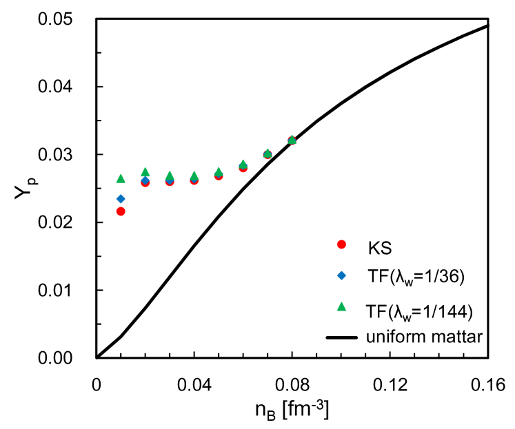
Figure 4: (Color online) Calculated proton ratio $Y_{p}$ for slab phase as a function of baryon density $n_{B}$. See the caption of Fig. 3.

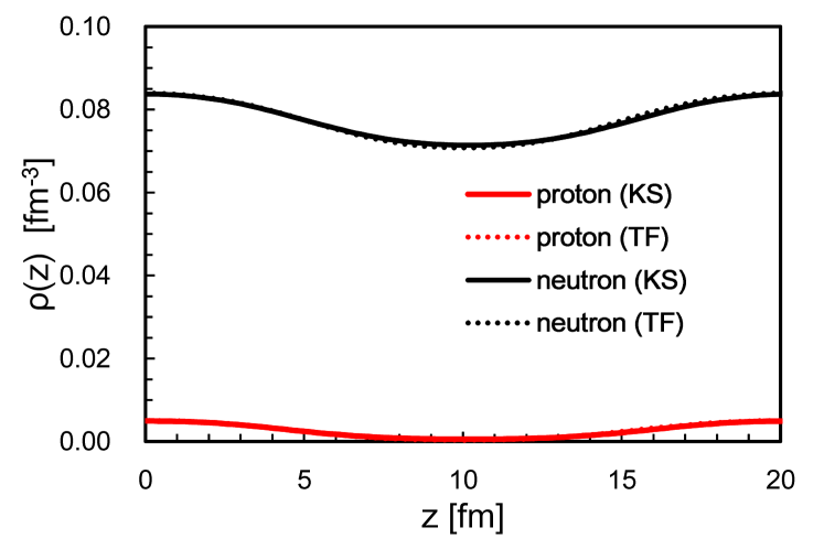
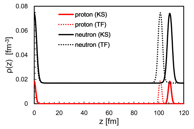
Figure 5: (Color online) Calculated neutron and proton density distributions in the slab phase as functions of $z$ at beta equilibrium. The results of TF approximation ($\lambda_{W}=1/36$) are shown by dashed lines. The top panel shows that at $n_{B}=0.08$ fm^-3, while the bottom one shows that at $n_{B}=0.02$ fm^-3. The left end ($z=0$) corresponds to the center of a slab. The obtained lattice constants are $a=20.0$ fm for both the band and TF calculations for the top panel, while they are $a=108.8$ fm (band) and $101.4$ fm (TF) for the bottom one.

III.3.1 Beta equilibrium

Let us first show comparison between the band calculation and the TF calculation at beta equilibrium. We calculate the slab phase at baryon density every 0.01 fm^-3, in a region of $0.01\leq n_{B}\leq 0.08$. At $n_{B}\geq(n_{B})^{c}$ with the critical density $(n_{B})^{c}=0.083$ fm^-3, the slab nuclei are dissolved to produce uniform nuclear matter in both calculations. In Fig. 3, we show the nuclear energy per nucleon $E_{B}/A$ which monotonically increases as the baryon density $n_{B}$ increases; $E_{B}/A=+2.7$ MeV at $n_{B}=0.01$ fm^-3 and $E_{B}/A=+6.3$ MeV at $n_{B}=0.08$ fm^-3. The energy gain from the uniform phase amounts to $E_{B}/A\approx 1$ MeV at maximum. The TF calculation well reproduces these values, especially near the critical density $n_{B}\sim(n_{B})^{c}$.

The calculated proton ratio $Y_{p}$ is shown in Fig. 4. $Y_{p}$ at beta equilibrium in the slab phase is around $Y_{p}\approx 0.02-0.03$. Because of this small value of $Y_{p}$, the neutrons are always dripped in the slab phase at beta equilibrium. The band calculation suggests monotonic increase of $Y_{p}$ as a function of density, and it reaches $Y_{p}=0.032$ at $n_{B}=0.08$ fm^-3. In the low-density side, it shows an approximate constant value of $Y_{p}\approx 0.026$ in a region of $0.02\leq n_{B}\leq 0.04$ fm^-3, and a sudden drop from $Y_{p}\approx 0.026$ at $n_{B}=0.02$ to $Y_{p}\approx 0.022$ at $n_{B}=0.01$ fm^-3. The TF calculation gives slightly larger $Y_{p}$ values, which is more prominent at lower density.

Figure 5 shows the one-dimensional density profiles. Qualitative features of the density profiles are well reproduced in the TF calculation, though we find some quantitative difference, especially at low density. The TF calculation always predicts the lattice constant $a$ smaller than the band calculation. This is probably due to the fact that the TF approximation underestimates the surface diffuseness. The TF calculation Oyamatsu (1993) predicted that the slab phase appears near the bottom of the inner crust of neutron star, at density around $n_{B}=0.07-0.09$ fm^-3. In such density region, since the difference is not so large, the TF description of the slab phase is reasonably good. In contrast, at lower density, the difference becomes larger. For instance, at $n_{B}=0.01$ fm^-3, the lattice constant of $a=199.6$ fm is predicted by the band calculation, while $a=176.2$ fm by the TF calculation.

In the uniform limit, the TF calculation exactly reproduces the result of the band calculation. Thus, it is natural to observe that the TF calculation well agrees with the band calculation at the uniform limit, $n_{B}\rightarrow 0.09$ fm^-3. The quantum effect missing in the TF calculation is more important at low baryon density $n_{B}$.

In order to see the effect of the Weizsäcker correction term in the TF calculation, we perform the same calculation with the prefactor reduced by $1/4$, $\lambda_{W}=1/144$. The energy $E_{B}/A$ is not sensitive to this change, however, the density profiles, the proton ratio $Y_{p}$, and the optimal slab interval $a$ are affected by the Weizsäcker term. The calculated proton ratio $Y_{p}$ are shown by triangles in Fig. 4. The deviation is larger at lower density.

Another feature we find in the band calculation is that not only neutrons but also protons are dripped from slab nuclei at $n_{B}\geq 0.08$ fm^-3. Near the transition to the uniform matter, the nuclear potential becomes almost flat. Thus, although protons are deeply bound with the chemical potential $\mu_{p}\approx-70$ MeV, $\mu_{p}$ can be larger than the maximum potential value for protons, $U_{p}^{0}$. This proton drip phenomenon does not take place in the TF calculation.

III.3.2 Fixed proton ratio

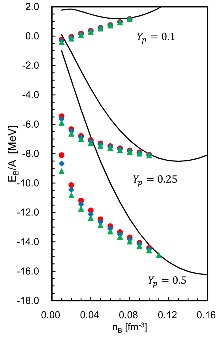
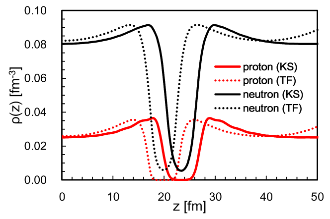
Figure 6: (Color online) Calculated nuclear energy per nucleon $E_{B}/A$ as functions of baryon density $n_{B}$, for the proton ratio $Y_{p}=0.5$, $Y_{p}=0.25$, and $Y_{p}=0.1$. The results of the TF calculation are shown by blue diamonds ($\lambda_{W}=1/36$) and by green triangles ($\lambda_{W}=1/144$), while those of the band calculation are by red circles. The solid lines show those of the uniform matter.

Figure 7: (Color online) The same as Fig. 5, but at $n_{B}=0.1$ fm^-3 and $Y_{p}=0.25$.

Away from the beta equilibrium, the discrepancy between the band and TF calculations becomes more prominent, especially when the lattice constant $a$ is large. We show, in Fig. 7, $E_{B}/A$ as functions of density $n_{B}$ for different values of proton ratio $Y_{p}$. At low density ($n_{B}=0.01$ fm^-3), the TF calculation underestimates $E_{B}/A$ by $\Delta(E_{B}/A)=0.58$ MeV for the symmetric slab case with $Y_{p}=0.5$. Adopting the reduced value of $\lambda_{W}=1/144$, the difference in $E_{B}/A$ becomes even larger, which amounts to 1.09 MeV. This discrepancy becomes smaller at higher density, however, the structure of the slab nuclei can be very different. As an example, we show the nucleons’ density profiles near the transition point from slab to uniform phase, in Fig. 7. The structure at $n_{B}=0.1$ fm^-3 with $Y_{p}=0.25$ is like “anti-slab” phase where gaps periodically appear in the uniform matter. Although the shapes of density distribution are somewhat similar, the lattice constant of the TF calculation is very different from that of the band calculation. In Fig. 7, the optimal lattice constant is $a=49.4$ fm for the band calculation, while $a=39.6$ fm for the TF calculation. A depression of density at the center of each slab, which appears for relatively high $Y_{p}$ values, is due to the Coulomb interaction among protons.

Increasing the baryon density, the slab phase changes into the uniform phase at a critical value of density. The band calculation indicates that this critical density $(n_{B})^{c}$ is located at between 0.1 and 0.11 fm^-3 for $Y_{p}=0.5$, and between 0.08 and 0.09 fm^-3 for $Y_{p}=0.1$. The quantum fluctuation tends to make the density distribution flatter, which leads to lower values of $(n_{B})^{c}$ than those of the TF approximation.

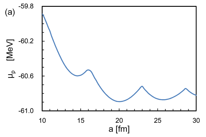
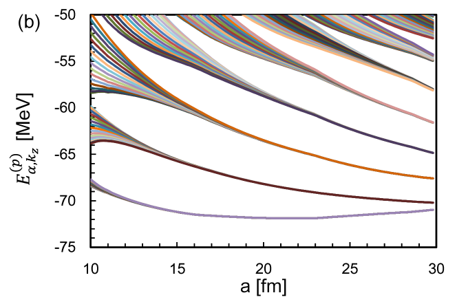
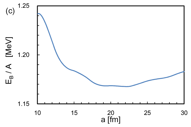
Figure 8: (Color online) (a) Calculated chemical potential for protons, (b) single-particle energies for protons, and (c) nuclear energy per baryon, as functions of lattice constant $a$, for the case of $Y_{p}=0.1$ and $n_{B}=0.08$ fm^-3. In the panel (b), each bundle of lines, which correspond to a single band index $\alpha$, contains 16 lines with different Bloch wave numbers $k_{z}$.

III.4 Band structure for slab phase

III.4.1 Proton shell effect

The shell effect is an obvious missing piece in the TF approximation. In the one-dimensional slab phase, Since all the nucleons have two-dimensional free motion in the $x-y$ directions, the shell effect is not so strong. Nevertheless, in most cases, the protons are bound in the $z$ direction and we expect some shell effect due to change of protons’ orbital occupancy.

In Fig. 8 (a), we show an example of the proton chemical potential $\mu_{p}$ as a function of the lattice constant $a$. It clearly shows ridges and multiple minima which are associated with the proton shells. The corresponding single-particle (band) energies $e^{(p)}_{\alpha,k_{z}}$ are shown in Fig. 8 (b). At the crossing points between the single-particle energy and the chemical potential, the chemical potential shows cusps. Although the proton shell effect is clearly visible in the chemical potential, the energy per baryon, $E_{B}/A$, still represents a smooth curve as in Fig. 8 (c). At the crossing points, we observe a kind of bending of the curve, with different slopes before and after the crossing. It should be noted that the proton single-particle energies $\epsilon_{\alpha,\bf{k}}$ in Eq. (9) are not discrete, because $k_{\rho}^{2}/2m_{p}$ is continuous.

The energies $e^{(p)}_{\alpha,k_{z}}$ should not depend on $k_{z}$ for bound protons. Therefore, the unraveled bundle of lines corresponds to dripped orbitals. Figure 8 (b) indicates that the protons start to drip from the slab nuclei at small $a$.

III.4.2 Band structure of neutrons

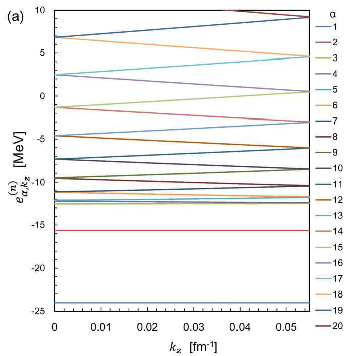
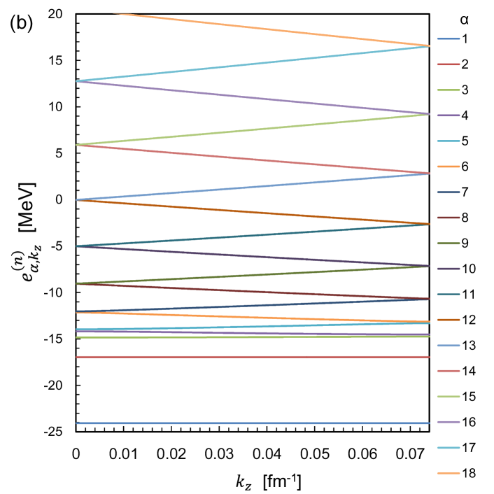
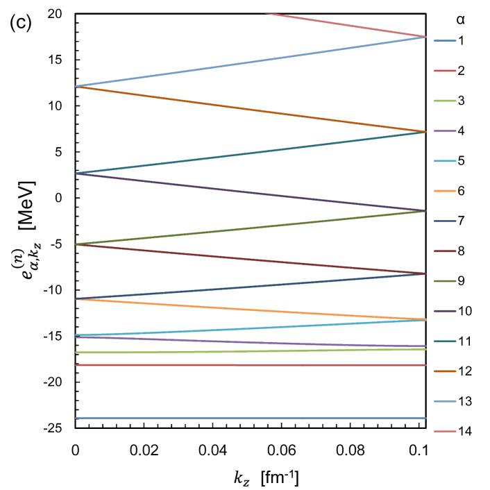
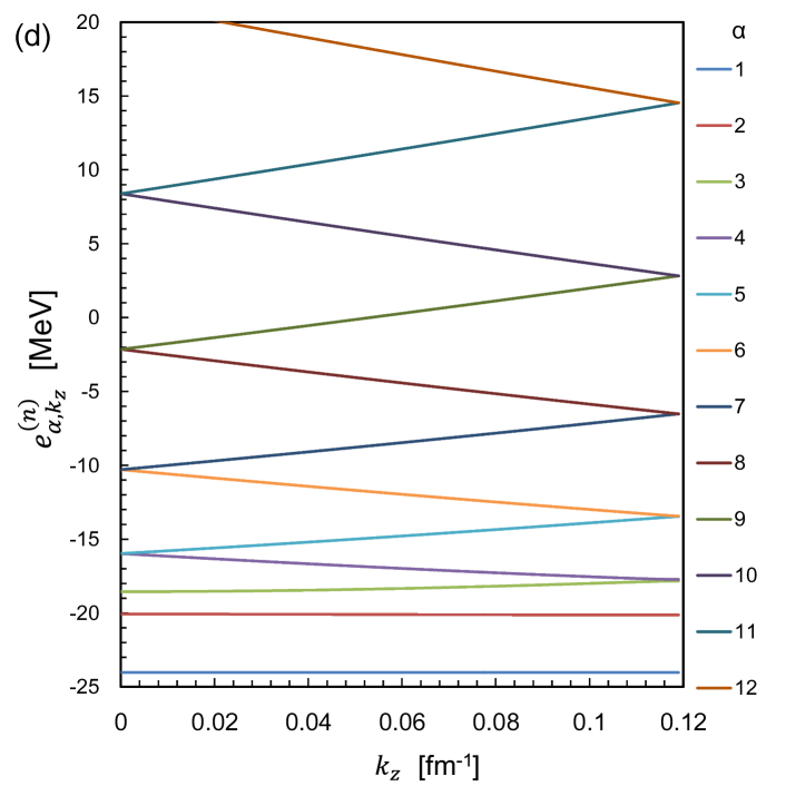
Figure 9: (Color online) Neutron band structure at beta equilibrium as a function of Bloch wave number $k_{z}>0$; (a) $n_{B}=0.04$ fm^-3, (b) $n_{B}=0.05$ fm^-3, (c) $n_{B}=0.06$ fm^-3, and (d) $n_{B}=0.07$ fm^-3. The lattice constants and neutron chemical potentials are given as (a) $a=56.4$ fm, $\mu_{n}=8.45$ MeV, (b) 42.2 fm, 9.55 MeV, (c) 30.8 fm, 10.71 MeV, (d) 26.4 fm, and 11.93 MeV, respectively. In each panel, the right end corresponds to the end point of the Brillouin zone $k_{z}=\pi/a$.

In the inner crust of neutron stars, the neutrons are partially dripped from the slabs. In Fig. 9, we show the band structure of neutrons at beta equilibrium. Since the band structure is symmetric with respect to the transformation of $k_{z}\rightarrow-k_{z}$, we show here only a half of the first Brillouin zone with positive $k_{z}$. At the center ($k_{z}=0$) and the end ($k_{z}=\pm\pi/a$) of first Brillouin zone, there are band gaps. The calculated band gaps are small in the slab phase, which are less than a few hundreds of keV. The magnitude of the band gap varies from band to band, however, typically it becomes smaller for bands with larger energies $e^{(n)}_{\alpha,k_{z}}$.

The effective mass (33) along the $z$ direction is shown in Fig. 10 for $n_{B}=0.04$ fm^-3. For bound neutrons with $e^{(n)}_{\alpha,k_{z}}<U_{n}^{0}$, we have $(1/m_{z}^{*})_{\alpha,k_{z}}^{zz}\approx 0$ which means that these neutrons have infinite mass, because they cannot “move” toward $z$ direction. Here, since we have $U_{n}^{0}=-12.57$ MeV, the lowest two bands correspond to these “core” neutrons with the infinite effective mass. This is also consistent with vanishing group velocity according to Eq. (30).

The dripped neutrons have finite values of effective mass. The lowest “valence” band ($e^{(n)}_{\alpha,k_{z}}>U_{n}^{0}$) is the third lowest one in Fig. 9(a). In Fig. 10), only this band shows the convergence of the effective mass to the bare mass ($1/m_{n}=1.06\times 10^{-3}$ MeV^-1) at $k_{z}\rightarrow 0$, while it becomes negative at $|k_{z}|>0.036$ fm^-1. If we apply a force on neutrons toward positive $z$ direction, those with negative effective mass would be accelerated toward negative $z$ direction. This is due to the Bragg scattering from the periodic potential. For high-lying bands, only at the vicinity of $k_{z}=0$ and $\pm\pi/a$, the effective mass shows deviation from the bare mass.

In solids with three-dimensional crystalline structure, the electrons in fully occupied bands do not contribute to the conduction current Ashcroft and Mermin (1976). This is because all the states in the band $\alpha$ are occupied, thus, the intraband excitations, $(\alpha,\mathbf{k})\rightarrow(\alpha,\mathbf{k}^{\prime})$, are not allowed. However, the situation is different in the slab phase embedded in the three-dimensional matter. Even for $e^{(n)}_{\alpha,k_{z}}<\mu_{n}$, there are still unoccupied states with the same $(\alpha,k_{z})$, because it is always possible to find the states with $\epsilon^{(n)}_{\alpha,\mathbf{k}}>\mu_{n}$ by increasing ${k}_{\rho}$, according to Eq. (9). Therefore, all the “valence” bands with finite velocity of the $z$ direction, $de^{(n)}_{\alpha,k_{z}}/dk_{z}\neq 0$, may contribute to the neutron current.

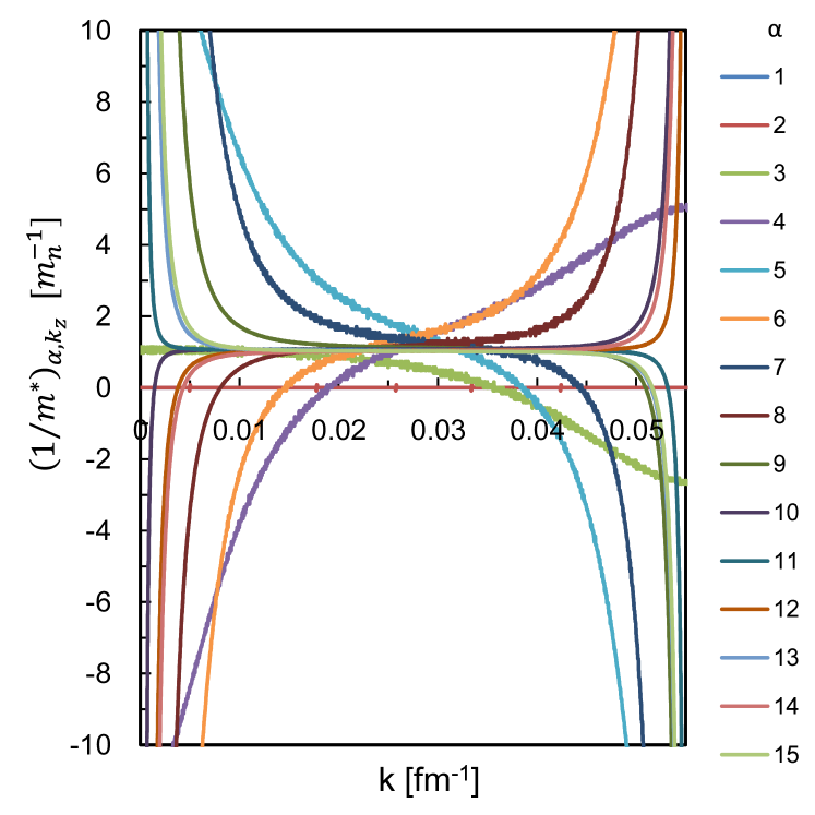
Figure 10: (Color online) Neutron effective mass $(1/m^{*})_{\alpha,k_{z}}^{zz}$ as a function of $k_{z}$, calculated at beta equilibrium with $n_{B}=0.04$ fm^-3. The colors correspond to those in Fig. 9(a).

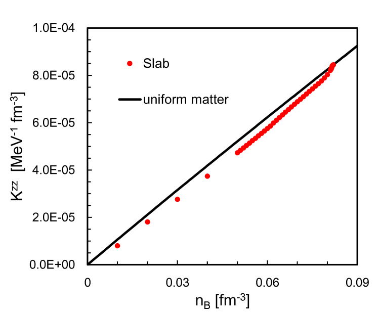
Figure 11: (Color online) Neutron mobility coefficient $\mathcal{K}^{zz}$ calculated at beta equilibrium as a function of density. Those of the uniform matter are shown by a solid line.

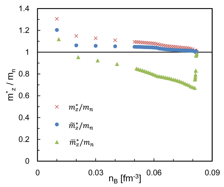
Figure 12: (Color online) Neutron effective masses $m_{z}^{*}$, $\bar{m}_{z}^{*}$, and $\tilde{m}_{z}^{*}$ calculated at beta equilibrium as functions of density.

III.4.3 Mobility and average effective mass of neutrons

In the uniform matter, the mobility coefficient (36) for neutrons is simply given as $\mathcal{K}^{zz}=n_{z}^{c}/m_{n}=n_{n}/m_{n}$, which is proportional to the total neutron density $n_{n}$. Since the proton ratio $Y_{p}$ is approximately constant at beta equilibrium, this simple relation leads to the dashed straight line in Fig. 11. In the slab phase, the mobility toward the $z$ direction is certainly reduced from that in the uniform matter. This directly affects the average effective mass $m_{z}^{*}$ of Eq. (39), which leads to $m_{z}^{*}/m_{n}\approx 1.0-1.3$, as a monotonically decreasing function of density $n_{B}$ (crosses in Fig. 12). A major origin of this effect comes from the existence of bound neutrons which are practically prevented from moving in the $z$ direction by the potential barrier, $e^{(n)}_{\alpha,k_{z}}<U_{n}^{0}$. These “core” neutrons exist inside the slab nuclei but are not present in the dripped low-density neutrons between the slabs.

In order to measure the mobility of these low-density neutrons dripped from the slab nuclei, we should calculate the density of “free” neutrons $n_{n}^{f}$ instead of the total neutron density $n_{n}$. According to the definition, Eqs. (40), and (41), $n_{n}^{f}$ are calculated. At beta equilibrium with $n_{B}\geq 0.83$ fm^-3, the calculation predicts the uniform phase in which we have $n_{n}^{f}=n_{n}$ because $U_{n}^{0}<e^{(n)}_{\alpha,k_{z}}$ for all $(\alpha,k_{z})$. $n_{n}^{f}$ monotonically decreases as decreasing $n_{B}$, then, reaches $\tilde{n}_{n}^{f}/n_{n}=0.922$ and $\bar{n}_{n}^{f}/n_{n}=0.856$ at $n_{B}=0.01$ fm^-3.

We show in Fig. 12 the average effective mass, $m_{z}^{*}$, $\tilde{m}_{z}^{*}$, and $\bar{m}_{z}^{*}$. For their definitions, see Eqs. (39) and (42). It turns out that the average effective mass depends on the definition of the free neutrons. All the three effective masses are larger than the bare neutron mass $m_{n}$ at very low density ($n_{B}\lesssim 0.01$ fm${}^{{}^{3}}$). However, we have $\bar{m}_{z}^{*}/m_{n}<1$ at $n_{B}\gtrsim 0.02$ fm^-3, thus, $m_{z}^{*}\geq\tilde{m}_{z}^{*}\geq m_{n}\geq\bar{m}_{z}^{*}$ in the region of $0.02<n_{B}<0.083$ fm^-3. Beyond the critical density $n_{B}>0.083$ fm^-3, all the effective masses are identical to the bare mass. Since we expect that the dripped neutrons between the slab nuclei consist of neutrons occupying states with $e^{(n)}_{\alpha,k_{z}}>U_{n}^{0}$, we suppose that $\bar{m}_{z}^{*}$ represents the mobility of the dripped low-density neutrons. They are calculated to be smaller than the bare mass. This means that the conduction neutron density is larger than that of free neutrons, $n_{z}^{c}>\bar{n}_{n}^{f}$. Thus, the entrainment effect for the dripped neutrons in the slab phase enhances the mobility of the dripped neutrons. This is opposite to our naive expectation. In the density region where the slab phase is expected ($0.07\leq n_{B}<0.08$ fm^-3) at beta equilibrium, the effective mass $\bar{m}_{z}^{*}$ is significantly smaller than the bare mass, $m_{z}^{*}/m_{n}=0.65\sim 0.75$.

Figure 12 shows the effective masses at the beta-equilibrium condition. However, away from the beta-equilibrium condition, these values can be much larger or smaller. For instance, at $n_{B}=0.04$ fm^-3 and $Y_{p}=0.25$, we obtain $m_{z}^{*}/m_{n}=16.2$, $\tilde{m}_{z}^{*}/m_{n}=2.8$, and $\bar{m}_{z}^{*}/m_{n}=0.53$. The average effective masses are about 30 times different, depending on their definition. This is because only a small fraction of neutrons are dripped in this case and the valence bands of $e^{(n)}_{\alpha,k_{z}}>U_{n}^{0}$ provide small effective masses. As we see in Fig. 12, the effective masses significantly vary from one band to another. Thus, depending on which band the neutrons belong to, they may differently respond to an external force.

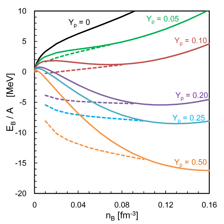
Figure 13: (Color online) Nuclear energy per baryon $E_{B}/A$ as functions of density $n_{B}$ for different values of $Y_{p}$. The dashed lines indicate $E_{B}/A$ of the slab nuclei, while the solid lines correspond to the uniform matter EOS.

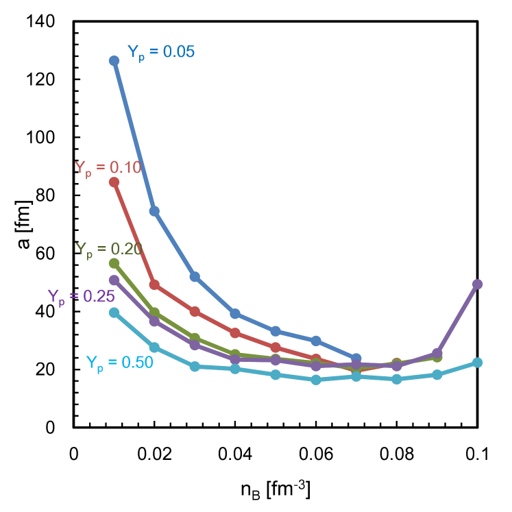
Figure 14: (Color online) Lattice constant $a$ as a function of density $n_{B}$. Different lines correspond to different values of proton ratio $Y_{p}$.

III.4.4 EOS of the slab phase

Calculated energy per baryon is summarized in Fig. 13. The non-uniform slab phase is favored at low density $n_{B}<0.1$ fm^-3. Especially at large $Y_{p}$, the non-uniform structure is strongly favored by reducing the Coulomb energy. At the lowest density, difference in $E_{B}/A$ between these two phases amounts to about 7 MeV. Of course, in such low-density region, we expect that other non-uniform phases, such as rod or droplet, are even more favored. The slab phase with $Y_{p}=0.5$ can be energetically most favored among various phases of nuclear pasta, in the density region of $0.05<n_{B}<0.07$ fm^-3 Okamoto et al. (2013). In this region, the energy gain is about 3 MeV per nucleon which is still significant. In contrast, the beta-equilibrium states with $Y_{p}=0.026$ at $n_{B}=0.03$ fm^-3 gain energy of $\Delta E_{B}/A\approx 862$ keV.

The obtained lattice constant $a$ is shown in Fig. 14. Around the density of $0.07\sim 0.08$ fm^-3, the calculated lattice constant is $a=20-30$ fm, irrespective of proton ratio $Y_{p}$. The lattice constant increases in both low-density and high-density sides. In the high-density side, in the vicinity of transition to uniform phase, the anti-slab-like structure appears and $a$ increases. In the low-density side, $a$ is significantly enhanced for systems with small $Y_{p}$. This can be understood as follows: For symmetric or near symmetric case with $Y_{p}\sim 0.5$, each slab has normal nuclear density and the neutrons never drip from the slab. Therefore, the lattice constant $a$ is basically determined by density $n_{B}$. The Coulomb energy favors larger values of $a$, but the given density $n_{B}$ forbids $a$ from being too large. In contrast, for small values of $Y_{p}$, since there exist dripped neutrons, a larger value of $a$ is allowed at a given density $n_{B}$.

IV Summary

The fully self-consistent band calculation based on the BCPM energy density functional has been performed for the slab phase of the inner crust of neutron stars. The lattice constant $a$ was determined by minimization of the total energy for each value of density $n_{B}$ and proton ratio $Y_{p}$. Comparing the result with that of Thomas-Fermi (TF) approximation, we have found that the TF qualitatively reproduces the slab structure of the self-consistent band calculation under the beta-equilibrium condition. This is partly because the slab nuclei have a shell effect weaker than the other phases, such as rod and droplet. However, away from the beta equilibrium, the lattice constant can be significantly different, especially near the boundary between the slab and uniform phases. The Weizsäcker term in the TF theory plays an important role. Without this term, the results even more deviate from the band calculation.

The band structure of neutrons are obtained from the present calculation. The calculated band gaps at $k_{z}=0$ and $\pm\pi/a$ are small, typically, order of keV to tens of keV. These values of the band gap are significantly smaller than magnitude of neutron pairing gap, which is expected to be order of hundreds of keV or MeV. The non-dissipative entrainment effect is studied by calculating the macroscopic effective mass due to the Bragg scattering. We have found that, the calculated mobility coefficient $\mathcal{K}^{zz}$ and equivalently the conduction neutron density $n_{z}^{c}$, are certainly reduced from the values for the uniform nuclear matter ($n_{z}^{c}<n_{n}$). However, the average effective mass of dripped neutrons $\bar{m}_{z}^{*}$ is smaller than the bare neutron mass. It is somewhat surprising that, the Bragg scattering enhances the mobility of dripped neutrons.

In former studies Carter et al. (2005); Chamel (2012), the calculated effective mass is always larger than the bare mass, $m^{*}/m_{n}>1$, in all the (pasta) phases of the inner crust. Their effective mass in the slab phase corresponds to $\tilde{m}_{z}^{*}$ of Eq. (42), whose values are consistent with our results, $\tilde{m}_{z}^{*}/m_{n}=1.0-1.05$ in the density region of $n_{B}\geq 0.07$ fm^-3. In this definition, the “free” neutrons include those in orbitals with $e^{(n)}_{\alpha,k_{z}}<U_{n}^{0}$ which are trapped inside the slab nuclei. Therefore, we suppose that the mobility of neutrons dripped from the slabs is better represented by the effective mass $\bar{m}_{z}^{*}$ rather than $\tilde{m}_{z}^{*}$.

We have performed the calculation for the one-dimensional slab phase without the pairing correlations. For the slab phase in the inner crust of neutron stars, we can conclude that the entrainment effect for neutrons does not influence the conventional interpretation of the pulsar glitches Anderson and Itoh (1975); Link et al. (1999); Andersson et al. (2012).

This is the first step for the fully self-consistent band calculation for the inner crust of neutron stars. Obviously, its extension to rod-like and crystalline nuclei with superfluid neutrons is highly desirable. In addition, there is an recent argument that the effect of the band structure is significantly hindered when the pairing gap $\Delta_{n}$ is greater than the band gap $\Delta\epsilon_{n}$ Watanabe and Pethick (2017). The present calculation for the slab phase is exactly the case, namely $\Delta\epsilon_{n}\ll\Delta_{n}$. In order to take account of the pairing and the temperature effect simultaneously, we are currently developing a parallelized computer program of the finite-temperature Hartree-Fock-Bogoliubov calculation with the three-dimensional coordinate-space representation. We plan to use this for our future studies of various phases in the inner crust.