Analysis of two-phase shape optimization problems by means of shape derivatives

A thesis submitted for the degree of
Doctor of Philosophy

by

Lorenzo Cavallina

Division of Mathematics
Graduate School of Information Sciences
Tohoku University

July 2018

Notations

Euclidean space

$\mathbb{N}$	the set of positive integers $\{1,2,3\dots\}$
$\mathbb{R}$	the set of real numbers
${{\mathbb{R}}^{N}}$	the $N$-dimensional Euclidean space, $N\geq 2$
$a\cdot b$	the inner product in ${{\mathbb{R}}^{N}}$, $\sum_{i=1}^{N}a_{i}b_{i}$
$\mathinner{\!\left\lVert x\right\rVert}$	the Euclidean norm, $\sqrt{x_{1}^{2}+\dots x_{N}^{2}}$, sometimes also used to denote a generic norm of some Banach space
${{\rm Id}}$	the identity map $x\mapsto x$
$B_{r}$	the open ball with radius $r>0$ centered at the origin
$\overline{A}$	the closure of the open set $A$
$\partial A$	the boundary of the open set $A$, given by $\overline{A}\setminus A$
$\int_{\Omega}f$	the integral of $f$ over $\Omega$ with respect to the $N$-dimensional Lebesgue measure
$\int_{\partial\Omega}f$	the (surface) integral of $f$ over $\partial\Omega$ with respect to the $(N-1)$-dimensional Hausdorff measure

Matrix notation

$\mathbb{R}^{N\times N}$	the set of real square matrices
$I$	the identity matrix
$\det A$	the determinant of the square matrix $A$
$\mathop{\mathrm{tr}}A$	the trace of the square matrix $A$
$A^{T}$	the transpose of $A$, $(A^{T})_{i,j}=A_{j,i}$
$A^{-1}$	the inverse of an invertible square matrix $A$
$A^{-T}$	the transpose of the inverse of $A$

Differential operators

${\nabla}f$	the gradient of the function $f$ with respect to the space variables $x_{i}$
$Dw$	the Jacobian matrix of the vector field $w$, $(Dw)_{i,j}=\frac{\partial w_{i}}{\partial x_{j}}$
${\mathop{\mathrm{div}}}w$	the divergence of the vector field $w$, given by $\mathop{\mathrm{tr}}Dw$
$D^{2}f$	the Hessian matrix of the function $f$, given by $(D^{2}f)_{i,j}=\frac{\partial^{2}f}{\partial x_{i}\partial x_{j}}$
$\Delta f$	the Laplace operator of the function $f$, given by $\mathop{\mathrm{tr}}D^{2}f$
${\nabla}_{\tau}f$	the tangential gradient of f, see Appendix A
${\mathop{\mathrm{div}}}_{\tau}w$	the tangential divergence of w, see Appendix A
$\Delta_{\tau}f$	the Laplace–Beltrami operator of f, see Appendix A
$\partial_{s}f$	the partial derivative of $f$ with respect to the variable $s$

Function spaces

$L^{p}(\Omega,\mathbb{R}^{M})$	the space of p-summable functions $\Omega\to\mathbb{R}^{M}$, $1\leq p\leq\infty$, endowed with the usual norm $\mathinner{\!\left\lVert{\boldsymbol{\cdot}}\right\rVert}_{p}$
$L^{p}(\Omega)$	abbreviate notation for $L^{p}(\Omega,\mathbb{R})$
$W^{k,p}(\Omega,\mathbb{R}^{M})$	the space of functions $\Omega\to\mathbb{R}^{M}$ whose partial derivatives up to the $k$-th order are p-summable, $1\leq p\leq\infty$, endowed with usual norm $\mathinner{\!\left\lVert{\boldsymbol{\cdot}}\right\rVert}_{k,p}$
$W^{k,p}(\Omega)$	abbreviate notation for $W^{k,p}(\Omega,\mathbb{R})$
$H^{1}(\Omega)$	alternative notation for $W^{1,2}(\Omega)$
$H_{0}^{1}(\Omega)$	the subset of $H^{1}(\Omega)$ of functions with vanishing trace on $\partial\Omega$
$\mathcal{C}^{k}(\Omega)$	the class of functions that are continuously differentiable $k$ times
$\mathcal{C}^{k,\infty}(\Omega)$	the space $\mathcal{C}^{k}(\Omega)\cap W^{k,\infty}(\Omega)$ endowed with the norm $\mathinner{\!\left\lVert{\boldsymbol{\cdot}}\right\rVert}_{k,\infty}$
$\mathcal{C}^{k+\alpha}(\Omega)$	the subclass of $\mathcal{C}^{k}(\Omega)$ made of functions whose $k$-th partial derivatives are Hölder continuous with exponent $\alpha\in(0,1]$

Chapter 1 Introduction and main results

Let $D\subset\Omega$ be a pair of bounded domains in the $N$-dimensional Euclidean space ${{\mathbb{R}}^{N}}$ ($N\geq 2$). Moreover, assume that $\overline{D}\subset\Omega$. In this way $\Omega$ gets partitioned into two subsets: $D$ and $\Omega\setminus D$ (from now on they will be referred to as core and shell respectively). Take two (possibly distinct) positive constants $\sigma_{c}$ and $\sigma_{s}$ and set

$$\sigma(x)=\sigma_{D,\Omega}(x)\mathrel{\mathop{\mathchar 58\relax}}=\left\{\begin{aligned} \sigma_{c}\quad&\text{ for }x\in D,&\text{{\em(core)}}\\ \sigma_{s}\quad&\text{ for }x\in\Omega\setminus D&\text{{\em(shell)}}.\end{aligned}\right.$$ (1.1)

Consider the following boundary value problem

$$\left\{\begin{aligned} -{\mathop{\mathrm{div}}}(\sigma{\nabla}u)&=1&\quad\text{ in }\Omega,\\ u&=0&\quad\text{ on }\partial\Omega.\end{aligned}\right.$$ (1.2)

We say that a function $u\in H_{0}^{1}(\Omega)$ is a solution of (1.2) if it verifies the following weak formulation:

$$\int_{\Omega}\sigma{\nabla}u\cdot{\nabla}\psi=\int_{\Omega}\psi\quad\text{ for all }\psi\in H_{0}^{1}(\Omega).$$ (1.3)

Since $\sigma$ attains a different value at each phase ($D$ and $\Omega\setminus D$), problems like (1.2) are usually called two-phase problems (of course, the term multi-phase is also used, when the phases are more than two). In the sequel, the subscripts $c$ and $s$ will be used to denote the restriction of any function to the core and the shell respectively, moreover we will also employ the use of the notation $[f]\mathrel{\mathop{\mathchar 58\relax}}=f_{c}-f_{s}$ to refer to the jump of a function $f\in L^{2}(\Omega)\cap H^{1}(D)\cap H^{1}(\Omega\setminus\overline{D})$ along the interface $\partial D$.

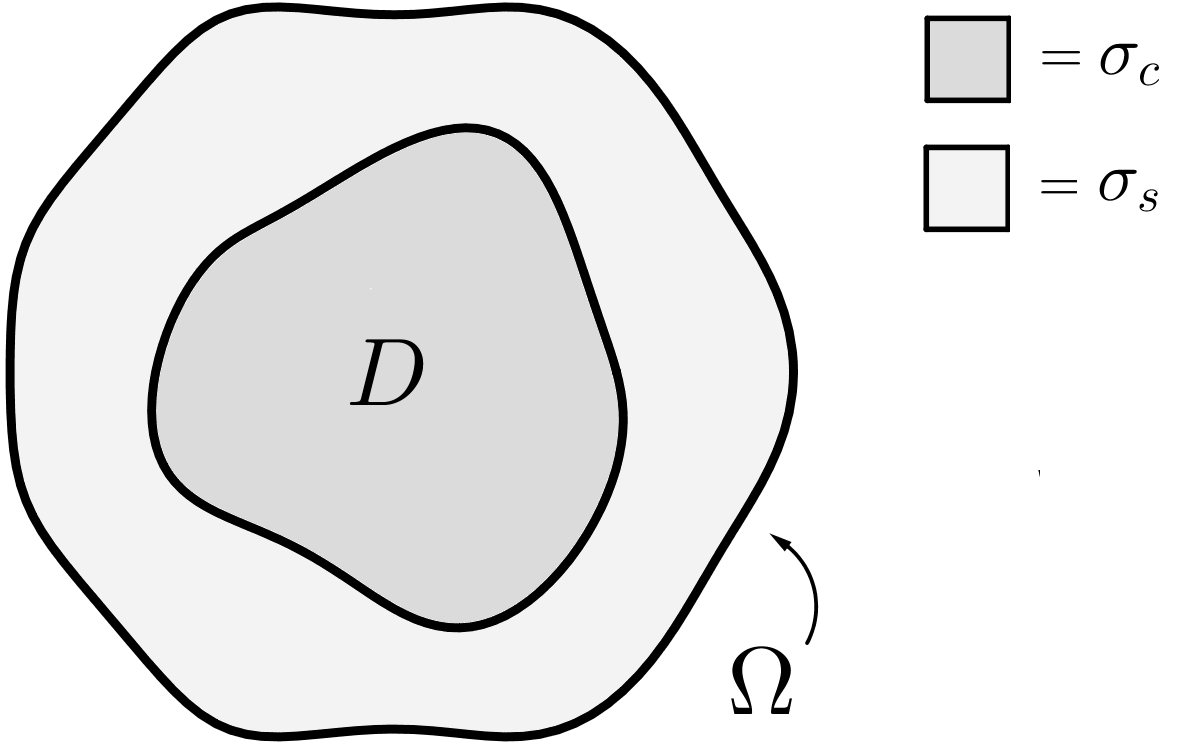
Figure 1: Our problem setting

When $\partial D$ and $\partial\Omega$ are at least of class $\mathcal{C}^{2}$, then the solution $u$ of problem (1.3) enjoys higher regularity, namely $u\in H_{0}^{1}(\Omega)\cap H^{2}(D)\cap H^{2}(\Omega\setminus\overline{D})$ (see [AS, Theorem 1.1]). Under these regularity assumptions on $D$ and $\Omega$, problem (1.3) admits the following alternative formulation (see [AS]):

$$\left\{\begin{aligned} -\sigma\Delta u&=1&\quad\text{ in }D\cup(\Omega\setminus\overline{D}),\\ [\sigma{\partial_{n}}u]&=0&\quad\text{ on }\partial D,\\ [u]&=0&\quad\text{ on }\partial D,\\ u&=0&\quad\text{ on }\partial\Omega.\end{aligned}\right.$$ (1.4)

Here, the letter $n$ is used indistinctly to refer to both the outward unit normal to $\partial D$ and $\partial\Omega$, and hence we will agree that, for smooth enough $f$, ${\partial_{n}}f={\nabla}f\cdot n$ stands the usual normal derivative (in the outward direction). The conditions

$$[\sigma{\partial_{n}}u]=[u]=0\quad\text{ on }\partial D$$ (1.5)

are usually called transmission conditions in the literature and therefore problems like (1.4), where the jump along the interface is prescribed, are usually referred to as transmission problems.

When $(D,\Omega)=(B_{R},B_{1})$, with $0<R<1$, then problem (1.4) admits an explicit radial solution:

$$u(x)=\begin{cases}\displaystyle\frac{1-R^{2}}{2N\sigma_{s}}+\frac{R^{2}-|x|^{2}}{2N\sigma_{c}}&\quad|x|\in[0,R],\\ \vspace*{-6mm}\\ \displaystyle\frac{1-|x|^{2}}{2N\sigma_{s}}&\quad|x|\in(R,1].\end{cases}$$ (1.6)

One of the main topics of this work is the study of the following functional

$$E(D,\Omega)\mathrel{\mathop{\mathchar 58\relax}}=\int_{\Omega}\sigma|{\nabla}u|^{2}=\int_{\Omega}u,$$ (1.7)

where $u$ is the solution of problem (1.2).

Physically speaking, the function $u$, solution to (1.2), plays the role of stress function while its integral, $E(D,\Omega)$, represents the torsional rigidity of an infinitely long composite beam $\Omega\times\mathbb{R}$ made of two different materials, such that their distribution is the one given in Figure 1 for each cross section $\Omega\times\{x_{N+1}\}$. The constants $\sigma_{c}$ and $\sigma_{s}$ are linked to the hardness of the materials in question (the smaller the constant, the harder the corresponding material, hence the higher the torsional rigidity $E(D,\Omega)$, as one can see by (1.7) and (1.2)).

The one-phase case (i.e. when $D=\emptyset$) was studied by Pólya by means of spherical rearrangement inequalities. In [Po], he proved that the ball maximizes the functional $E(\emptyset,{\boldsymbol{\cdot}})$ among all open sets of a given volume (see Theorem 2.1). Unfortunately, the methods employed by Pólya do not generalize well to a two-phase setting. We decided to perform a local analysis of the functional $E({\boldsymbol{\cdot}},{\boldsymbol{\cdot}})$ by means of shape derivatives. Inspired by the work of Pólya, we aim to find the relationship between the radial symmetry of the configuration $(D,\Omega)$ and local optimality for the functional $E$. The following theorem is one of our original results, concerning the first order shape derivative of $E$. From now on, let $(D_{0},\Omega_{0})$ denote a pair of concentric balls $(B_{R},B_{1})$ with $0<R<1$.

Theorem I ([Ca2]).

The pair $(D_{0},\Omega_{0})$ is a critical shape for the functional $E$ under the fixed volume constraint.

Theorem I can be improved by looking at second order shape derivatives. Exact computations are carried on with the aid of spherical harmonics at the end of Chapter 4. We get the following symmetry breaking result.

Theorem II ([Ca2]).

The pair $(D_{0},\Omega_{0})$ is a local maximum for the functional $E$ under the fixed volume and barycenter constraint if $\sigma_{c}\geq\sigma_{s}$, otherwise it is a saddle shape.

Theorem II shows a substantial difference between the one-phase maximization problem studied by Pólya and our two-phase analogue. As a matter of fact, as we will show in Section 3.5, the one-phase functional $E(\phi,{\boldsymbol{\cdot}})$ subject to the volume preserving constraint does not possess any critical point other than its global maximum.

An obvious observation concerning the radially symmetric configuration $(D_{0},\Omega_{0})$ is the following: the related stress function $u$ is itself radially symmetric and thus its normal derivative is constant on $\partial\Omega_{0}$. It is well known that, when $D=\emptyset$ then this property characterizes the ball. In [Se] Serrin showed that if the stress function corresponding to $(\emptyset,\Omega)$ has a normal derivative that is constant on the boundary $\partial\Omega$, then $\Omega$ must be a ball (see Theorem 2.4). The original proof by Serrin is based on an ingenious adaptation of Aleksandrov’s reflection principle (see [Al]) nowadays referred to as method of moving planes. This technique takes advantage of the invariance properties that characterize the Laplace operator and thus cannot be extended to our two-phase setting in any obvious way. It is not even clear at first glance whether an analogous characterization of the two-phase radial configuration $(D_{0},\Omega_{0})$ holds true. For $\beta\geq 0$ and $\gamma>0$ we consider the following overdetermined problem

$$\left\{\begin{aligned} {\rm div}(\sigma{\nabla}u)&=\beta u-\gamma&\text{ in }\Omega,\\ u&=0&\text{ on }\partial\Omega,\\ \sigma_{s}\partial_{n}u&=-d&\text{ on }\partial\Omega,\end{aligned}\right.$$ (1.8)

where $d$ is a positive constant to be determined, depending on the geometry of the solution $(D,\Omega)$. By means of a perturbation argument based on the implicit function theorem for Banach spaces, we manage to disprove the analogue of Serrin’s result for the operator $-{\mathop{\mathrm{div}}}\left(\sigma{\nabla}{\boldsymbol{\cdot}}\right)$.

Theorem III ([CaMS]).

For all domain $\Omega$ of class $\mathcal{C}^{2+\alpha}$ sufficiently close to $\Omega_{0}$ there exists a $\mathcal{C}^{2+\alpha}$-domain $D$ close to $D_{0}$ such that $(D,\Omega)$ is a solution to the overdetermined problem (1.8). In particular, there are infinitely many non radially symmetric solutions $(D,\Omega)$ of problem (1.8) with $D$ and $\Omega$ of class $\mathcal{C}^{2+\alpha}$.

As a final remark, notice that by a scaling argument, it is enough to prove Theorems I–III under the assumption that $\sigma_{s}=1$. Therefore, in what follows we will always assume $\sigma_{s}=1$.

As the title of this thesis suggests, shape derivatives will be our main tool. The concept of differentiating a shape functional with respect to a varying domain is actually really old. It dates back to the beginning of the $20$th century with the pioneering work of Hadamard [Ha]. It is virtually impossible to give an exhaustive list of all the contributions that have been made to this theory. We refer to the monographs [DZ, HP] for some good introductory material on the classical theory of shape derivatives and shape optimization in general. Among others, we would like to refer to [HL, NP, Si] for their theoretical contributions and the related formalism. Moreover, one can not avoid mentioning works like [CoMS] or [DK] where shape derivatives are used to investigate the local optimality of concentric balls for some two-phase eigenvalue problem (which is deeply related to the two-phase torsional rigidity functional $E$). As a final note, we might as well point the potential applications of this theory to the realm of numerical shape optimization (see for instance [CZ] and [CDKT]).

This thesis is organized as follows. In Chapter 2 we discuss the proofs of the classical results by Pólya [Po] and Serrin [Se] that take place in a one-phase setting. Chapter 3 provides the necessary theoretical background about shape derivatives. We used [HP] as the main reference here. Chapter 4 is devoted to the exposition of our first original result: the detailed analysis of the first and second order shape derivative of the functional $E$ and the subsequent proof of Theorems I–II (see [Ca1, Ca2]). Finally, the two-phase overdetermined problem of Serrin-type (1.8) is analyzed in Chapter 5, where Theorem III is proved by the implicit function theorem (see [CaMS]).

Chapter 2 Classical results in the one-phase setting

2.1 Optimal shape for the torsional rigidity

For all open sets $\Omega\subset{{\mathbb{R}}^{N}}$ of finite volume we denote by $\Omega^{*}$ the ball centered at the origin whose volume agrees with $\Omega$:

$$\Omega^{*}\mathrel{\mathop{\mathchar 58\relax}}=\left\{x\in{{\mathbb{R}}^{N}}\;\middle|\;{\rm Vol}(B_{1})|x|^{N}<{\rm Vol}(\Omega)\right\}.$$ (2.1)

In [Po], Pólya gave a very elegant proof of the following result.

Theorem 2.1.

For all open sets $\Omega\subset{{\mathbb{R}}^{N}}$ of finite volume, the following holds

$$E(\emptyset,\Omega)\leq E(\emptyset,\Omega^{*})$$

Actually the original proof by Pólya employed the use of the following equivalent definition of the (one-phase) torsional rigidity of an open set $\Omega$:

$$T(\Omega)\mathrel{\mathop{\mathchar 58\relax}}=\max_{v\in H_{0}^{1}(\Omega)\setminus\{0\}}\frac{\left(\int_{\Omega}|v|\right)^{2}}{\int_{\Omega}|{\nabla}v|^{2}}.$$ (2.2)

In order to prove the equivalence between the functionals $E(\emptyset,{\boldsymbol{\cdot}})$ and $T({\boldsymbol{\cdot}})$, we will follow [Bra] and introduce a third functional that will serve as a bridge between the two:

$$\mathcal{F}_{\Omega}(v)\mathrel{\mathop{\mathchar 58\relax}}=2\int_{\Omega}v-\int_{\Omega}|{\nabla}v|^{2}\quad\text{ for }v\in H_{0}^{1}(\Omega).$$ (2.3)

We will also need the following simple lemma. It follows immediately from Young’s inequality for products and therefore the proof will be omitted.

Lemma 2.2.

Let $A,B>0$, then we have

$$At-B\frac{t^{2}}{2}\leq\frac{A^{2}}{2B}\quad\text{ for }t\geq 0,$$ (2.4)

and equality in (2.4) holds only for $t=A/B$.

Lemma 2.3.

Let $\Omega\subset{{\mathbb{R}}^{N}}$ be an open set of finite volume. Then

$$E(\emptyset,\Omega)=\max_{v\in H_{0}^{1}(\Omega)}\mathcal{F}_{\Omega}(v)=T(\Omega).$$

Proof.

First of all, let us prove that $E(\emptyset,{\boldsymbol{\cdot}})=\max_{v\in H_{0}^{1}(\Omega)}\mathcal{F}_{\Omega}(v)$. Since $\mathcal{F}_{\Omega}$ is a strictly concave functional, it has a unique maximizer, say $v_{M}\in H_{0}^{1}(\Omega)$. Moreover, by computing its Gâteaux derivative, we get

$$0=\lim_{t\to 0}\frac{\mathcal{F}_{\Omega}(v_{M}+t\psi)-\mathcal{F}_{\Omega}(v_{M})}{t}=2\int_{\Omega}\psi-2\int_{\Omega}{\nabla}v_{M}\cdot{\nabla}\psi\quad\text{ for all }\psi\in H_{0}^{1}(\Omega).$$

In other words, $v_{M}$ is a weak solution of (1.3) for $D=\emptyset$ and $\sigma_{s}=1$. This implies that

$$E(\emptyset,\Omega)=\max_{v\in H_{0}^{1}(\Omega)}\mathcal{F}_{\Omega}(v).$$

Let now $v_{0}$ be a maximizer in (2.2) (which, without loss of generality, we will suppose non negative). Set

$$\lambda_{0}\mathrel{\mathop{\mathchar 58\relax}}=\frac{\int_{\Omega}v_{0}}{\int_{\Omega}|{\nabla}v_{0}|^{2}}.$$

It is not difficult to show that $w_{0}\mathrel{\mathop{\mathchar 58\relax}}=\lambda_{0}v_{0}\in H_{0}^{1}(\Omega)$ is a maximizer for $\mathcal{F}_{\Omega}$. Indeed, by Lemma 2.2 and definitions (2.2) and (2.3) we can write, for all $v\in H_{0}^{1}(\Omega)$,

$$\mathcal{F}_{\Omega}(v)=2\int_{\Omega}v-\int_{\Omega}|{\nabla}v|^{2}\leq 2\max_{\lambda\geq 0}\left\{\lambda\int_{\Omega}|v|-\frac{\lambda^{2}}{2}\int_{\Omega}|{\nabla}v|^{2}\right\}=\frac{\left(\int_{\Omega}|v|\right)^{2}}{\int_{\Omega}|{\nabla}v|^{2}}\leq T(\Omega).$$

Notice that equality holds in the chain of inequalities above if $v=\lambda_{0}v_{0}$. In particular, $\mathcal{F}_{\Omega}(v)\leq T(\Omega)=\mathcal{F}_{\Omega}(\lambda_{0}v_{0})$ for all $v\in H_{0}^{1}(\Omega)$ and therefore

$$E(\emptyset,\Omega)=\max_{v\in H_{0}^{1}(\Omega)}\mathcal{F}_{\Omega}(v)=\mathcal{F}_{\Omega}(\lambda_{0}v_{0})=T(\Omega),$$

which concludes the proof. ∎

The key to Pólya’s proof lies in spherical rearrangements of measurable functions and the related inequalities. Let $f$ be a nonnegative measurable function vanishing at infinity, in the sense that all its positive superlevel sets $\{f>t\}$ with $t>0$ have finite measure. We define its spherical decreasing rearrangement $f^{*}$ as the measurable function whose superlevel lets are the $*$-symmetrization of those of $f$ (see (2.1)):

$$\{f^{*}>t\}\mathrel{\mathop{\mathchar 58\relax}}=\{f>t\}^{*}\quad\text{ for all }t>0.$$ (2.5)

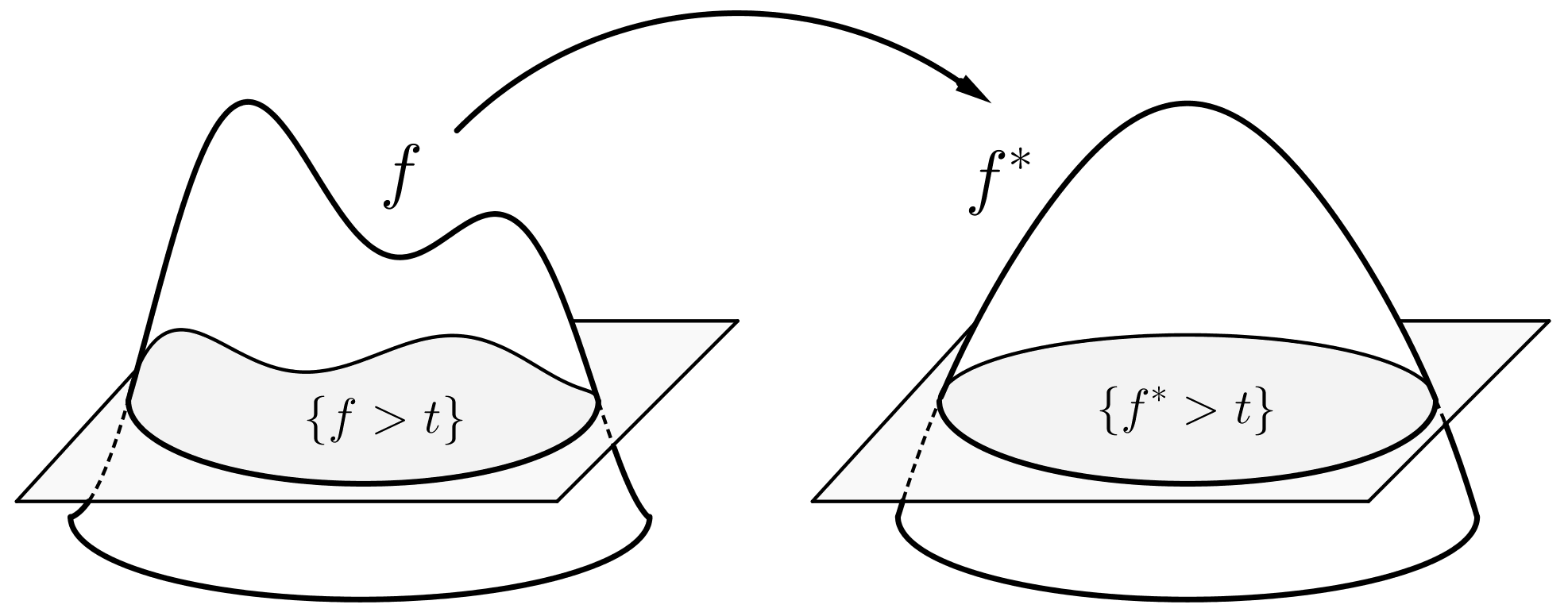
Figure 2: Spherical decreasing rearrangement.

Such function $f^{*}$ is uniquely determined by the measure of the superlevel sets of $f$ and admits the following “layer cake” decomposition:

$$f^{*}=\int_{0}^{\infty}\chi_{\{{f>t}\}^{*}}\,dt.$$

By (2.5) and Cavalieri’s principle, it follows that $f$ and $f^{*}$ are equimeasurable, i.e. for every measurable function $g\mathrel{\mathop{\mathchar 58\relax}}[0,\infty)\to\mathbb{R}$ the following holds

$$\int_{{\mathbb{R}}^{N}}g\circ f=\int_{{\mathbb{R}}^{N}}g\circ f^{*}.$$

In particular, this implies that $L^{p}$-norms are preserved after spherical rearrangements, in the sense that, if $f\in L^{p}({{\mathbb{R}}^{N}})$, $1\leq p\leq\infty$, is a nonnegative function vanishing at infinity, then

$$\mathinner{\!\left\lVert f\right\rVert}_{p}=\mathinner{\!\left\lVert f^{*}\right\rVert}_{p}.$$

On the other hand, the $L^{p}$-norm of the gradient is not preserved by spherical rearrangements, as the following result shows.

Theorem A (Pólya-Szegő inequality).

Let $f\in W^{1,p}({{\mathbb{R}}^{N}})$, $1\leq p\leq\infty$, be a nonnegative measurable function vanishing at infinity, then

$$\mathinner{\!\left\lVert{\nabla}f\right\rVert}_{p}\geq\mathinner{\!\left\lVert{\nabla}f^{*}\right\rVert}_{p}.$$

Proof of Theorem 2.1.

Once all the ingredients are ready, the proof just takes one line. Let $\Omega$ be a measurable set of finite measure and set $v_{0}\in H_{0}^{1}(\Omega)$ to be the maximizer in the definition of $T(\Omega)$. We have

$$T(\Omega)=\frac{\left(\int_{\Omega}v_{0}\right)^{2}}{\int_{\Omega}|{\nabla}v_{0}|^{2}}\leq\frac{\left(\int_{\Omega^{*}}v_{0}^{*}\right)^{2}}{\int_{\Omega^{*}}|{\nabla}v_{0}^{*}|^{2}}\leq T(\Omega^{*}),$$

where we used equimeasurability and Theorem A in the first inequality. ∎

2.2 Serrin’s overdetermined problem

In this section we will deal with the original one-phase Serrin’s overdetermined problem. We are looking for a bounded domain $\Omega\subset{{\mathbb{R}}^{N}}$ of class $\mathcal{C}^{2}$ such that the following overdetermined boundary value problem admits a solution for some constant $d$:

$$\left\{\begin{aligned} -\Delta u&=1&\quad\text{ in }\Omega,\\ u&=0&\quad\text{ on }\partial\Omega,\\ {\partial_{n}}u&=-d&\quad\text{ on }\partial\Omega.\end{aligned}\right.$$ (2.6)

In [Se], Serrin proved the following theorem, characterizing the solutions to (2.6).

Theorem 2.4.

Let $\Omega\subset{{\mathbb{R}}^{N}}$ be a bounded domain of class $\mathcal{C}^{2}$. If the overdetermined problem (2.6) admits a solution for some constant $d>0$, then $\Omega$ is an open ball of radius $R=Nd$.

If (2.6) has a solution, then, $d$ must be positive by the Hopf lemma. Moreover, by the divergence theorem

$$d=\frac{{\rm Vol}(\Omega)}{{\rm Per}(\Omega)},$$

and thus if $\Omega=B_{R}$, then $d=R/N$. On the other hand, the fact balls are the only domains that allow for a solution to problem (2.6) in not obvious at all. This has led many mathematicians to devise their own proofs: each of them shedding light on the problem from a different angle. In what follows, we will present the original proof by Serrin, nevertheless, the interested reader is encouraged to read the survey papers [Ma] and [NT]. Serrin’s proof heavily relies on the invariance with respect to rigid motions of the Laplace operator and on the maximum principle. In particular, both the classical Hopf lemma and the following refined version for domains with corners (see [Se] for a proof) play a fundamental role in the proof of Theorem 2.4.

Lemma B (Serrin’s corner lemma, [Se]).

Let $\Omega\subset{{\mathbb{R}}^{N}}$ be a bounded domain of class $\mathcal{C}^{2}$. Fix a point $P\in\partial\Omega$ and let $\theta$ be a direction orthogonal to $n(P)$ (the outward unit normal to $\partial\Omega$ at $P$). Moreover, let $H_{\theta}$ be an open half-plane that is orthogonal to $\theta$ and such that $\Omega\cap H_{\theta}\neq\emptyset$. Let $w\in\mathcal{C}^{2}(\overline{\Omega}\cap\overline{H}_{\theta})$ satisfy

$$-\Delta w\geq 0\quad\text{ and }w\geq 0\quad\text{ in }\Omega\cap H_{\theta}.$$

If $w(P)=0$, then, for all directions $\ell$ in $P$ entering $\Omega\cap H_{\theta}$, i.e. such that $\ell\cdot n<0$ at $P$, then

$$\text{ either }\;\partial_{\ell}w(P)>0\quad\text{ or }\quad\partial_{\ell\ell}w(P)>0,$$

unless $w\equiv 0$ in $\Omega\cap H_{\theta}$.

Proof of Theorem 2.4.

Serrin’s proof is based on the following idea: a domain $\Omega$ is a ball if and only if it is mirror-symmetric with respect to any fixed direction $\theta$. Suppose by contradiction that $\Omega$ is not mirror-symmetric in the direction $\theta$ (which, up to a rotation, can be assumed to be the upward vertical direction). Take now a hyperplane $\pi$ perpendicular to $\theta$ that does not intersect $\Omega$ (this can be done because $\Omega$ is bounded). Now, move $\pi$ along the direction $\theta$ until it intersects $\Omega$. Let ${\mathcal{S}}$ denote the portion of $\Omega$ that lies below the hyperplane and ${\mathcal{S}}^{\prime}$ its mirror-symmetric image with respect to it. If ${\mathcal{S}}^{\prime}\subset\Omega$, then we can continue moving the hyperplane upwards. This motion will eventually stop, namely when (at least) one of the two following cases occur (see Figure 3):

1. ${\mathcal{S}}^{\prime}$ becomes internally tangent to $\partial\Omega$ at some point $P\in\partial\Omega\setminus\pi$

2. the hyperplane $\pi$ is orthogonal to $\partial\Omega$ at some point $P\in\partial\Omega\cap\pi$.

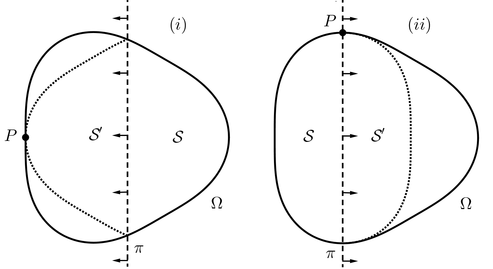
Figure 3: The method of moving planes: case (i) on the left, case (ii) on the right.

For all $x\in{{\mathbb{R}}^{N}}$, let $x^{\prime}$ denote the reflection of $x$ across the hyperplane $\pi$. We define the following auxiliary function on ${\mathcal{S}}^{\prime}$:

$$u^{\prime}(x)\mathrel{\mathop{\mathchar 58\relax}}=u(x^{\prime})\quad\text{ for }x\in{\mathcal{S}}^{\prime}.$$

Consider now the function $w\mathrel{\mathop{\mathchar 58\relax}}=u-u^{\prime}$ in ${\mathcal{S}}^{\prime}$. It is easy to see that $w$ verifies

$$\Delta w=0\,\text{ in }{\mathcal{S}}^{\prime},\quad w=0\,\text{ on }\partial{\mathcal{S}}^{\prime}\cap\pi,\quad w\geq 0\,\text{ on }\partial{\mathcal{S}}^{\prime}\setminus\pi,$$

where we applied the maximum principle to $u$ in order to obtain the last inequality. A further application of the maximum principle yields either $w>0$ in ${\mathcal{S}}^{\prime}$ or $w\equiv 0$ in ${\mathcal{S}}^{\prime}$. The latter is excluded because we are supposing by contradiction that $\Omega$ is not symmetric with respect to $\theta$. Assume now that case (i) occurs, that is ${\mathcal{S}}^{\prime}$ is internally tangent to $\partial\Omega$ at some point $P$ that does not belong to $\pi$. Then, by the Hopf lemma,

$${\partial_{n}}w(P)<0,$$

but by construction

$${\partial_{n}}w(P)={\partial_{n}}u(P)-{\partial_{n}}u^{\prime}(P)=-d+d=0.$$ (2.7)

In other words case (i) cannot occur if $\Omega$ is not symmetric with respect to $\pi$. Suppose now that case (ii) happens. In this case the Hopf lemma is not enough and we will resort to Lemma B. We are going to prove that, under these circumstances, the point $P$ is a second order zero for $w$, i.e. $w$ and all its first and second order derivatives computed at $P$ vanish. If this is the case, then by Lemma B, $w\equiv 0$ in ${\mathcal{S}}^{\prime}$, which is a contradiction. We will now show that $P$ is a second order zero for the function $w$. To this end, let us consider a coordinate system with the origin at $P$, the $x_{N}$ axis pointing in the direction $\theta$ and the $x_{1}$ axis in the direction of $n$. Locally there exists a $\mathcal{C}^{2}$-function $f\mathrel{\mathop{\mathchar 58\relax}}\mathbb{R}^{N-1}\to\mathbb{R}$ such that a portion of $\partial\Omega$ is given by

$$\left(f(x_{2},\dots,x_{N}),x_{2},\dots,x_{N}\right)\quad\text{ for }\mathinner{\!\left\lVert(x_{2},\dots,x_{N})\right\rVert}\text{ small}.$$

Therefore, $u\equiv 0$ on $\partial\Omega$ can be locally rewritten as

$$u(f,x_{2},\dots,x_{N})=0,$$ (2.8)

and since the outward normal $n$ admits the local expression

$$n(f,x_{2},\dots,n_{N})=\frac{\left(1,-{\partial_{x_{2}}}f,\dots,-\partial_{x_{N}}f\right)}{\sqrt{1+\sum_{i=2}^{N}(\partial_{x_{i}}f)^{2}}},$$

the overdetermined condition ${\partial_{n}}u=-d$ on $\partial\Omega$ is locally expressed by

$$\partial_{x_{1}}u-\sum_{i=2}^{N}\partial_{x_{i}}u\partial_{x_{i}}f=-d\bigg{\{}1+\sum_{i=2}^{N}\left(\partial_{x_{i}}f\right)^{2}\bigg{\}}^{1/2}.$$ (2.9)

Differentiating (2.8) with respect to $x_{i}$, $i=2,\dots,N$, yields

$$\partial_{x_{1}}u\partial_{x_{i}}f+\partial_{x_{i}}u=0.$$ (2.10)

Evaluate now (2.10) and (2.9) at $P$. Since $\partial_{x_{i}}f(0)=0$ for $i=2,\dots,N$, we have

$$\partial_{x_{1}}u(P)=-d,\quad\partial_{x_{i}}u(P)=0\,\text{ for }i=2,\dots,N.$$ (2.11)

This means that ${\partial_{n}}u=-d$ and ${{{\nabla}}_{\tau}}u=0$ at $P$, in other words, all first derivatives of $u$ and $u^{\prime}$ coincide at $P$, hence ${\nabla}w(P)=0$. In order to show that also $D^{2}w(P)=0$, notice that, in the new coordinates

$$u^{\prime}(x_{1},\dots,x_{N-1},x_{N})=u(x_{1},\dots,x_{N-1},-x_{N}).$$

In particular, by construction

$$\partial_{x_{N}x_{N}}u(P)=(-1)^{2}\partial_{x_{N}x_{N}}u^{\prime}(P)\;\text{ and }\;\partial_{x_{i}x_{j}}u(P)=\partial_{x_{i}x_{j}}u^{\prime}(P),\,i,j=1,\dots,N-1.$$ (2.12)

We are now left to show that all mixed derivatives with respect to $x_{i}$ and $x_{N}$ ($i=1,\dots,N-1$) of $u$ and $u^{\prime}$ coincide as well. Differentiate (2.10) with respect to $x_{N}$

$${\partial_{x_{i}x_{N}}}u(P)=d\,\partial_{x_{i}x_{N}}f(0)=0\quad i=2,\dots,N-1,$$ (2.13)

In the second equality above we used the assumption that the reflected cap ${\mathcal{S}}^{\prime}$ lies inside $\Omega$ and, therefore, $\partial_{x_{i}x_{N}}f(0)=0$ for $i=2,\dots,N-1$. We now need to compute $\partial_{x_{1}x_{N}}u$ at $P$. To this end, differentiate (2.9) with respect to $x_{1}$ and use (2.7). We get

$$\partial_{x_{1}x_{N}}u(P)=0$$ (2.14)

as claimed. We have proved that all the second order derivatives of $u$ and $u^{\prime}$ coincide at $P$. As remarked before, this contradicts the assumption that $\Omega$ is not mirror symmetric with respect to the hyperplane $\pi$, concluding the proof. ∎

Chapter 3 Shape derivatives

In this chapter we are going to introduce the concept of shape derivatives and some of the basic techniques in order to compute them. The contents of this chapter are well known classical results: we will follow [HP] and [DZ] in our exposition.

It is not unusual to encounter functions that depend on the “shape” of a domain $\omega$: the volume of $\omega$, its surface area, its barycenter or even the solution $u_{\omega}$ of some boundary value problem on $\omega$ etc… they are all shape functionals and the machinery in this chapter will apply to them all. In what follows, we will study how to deduce optimality conditions for shape functionals. As one knows, in order to find the extremal points of a function $f\mathrel{\mathop{\mathchar 58\relax}}{{\mathbb{R}}^{N}}\to\mathbb{R}$, one could resort to studying the points where its gradient ${\nabla}f$ vanishes. When the input variable of $f$ is not a point in the Euclidean space but a “shape” (for example an open set), then the above operation will lead to some overdetermined free boundary problem (we will discuss how this relates to the examples in Chapter 2 in Section 3.5). Nevertheless, it is not clear at first glance how the concept of derivative could be extended to shape functionals. We will give two (equivalent) formulations of this in Section 3.1. The actual computation techniques will be discussed in Section 3.2, where integral functionals (both on variable domains and on variable boundaries) will be of particular importance. Finally, in Section 3.4 it will be discussed how to compute shape derivatives of functionals that take values in a Banach space, in particular, we will be interested in how to compute the shape derivative $u^{\prime}$ of a functional of the form $\omega\mapsto u_{\omega}$, where $u_{\omega}$ solves some boundary value problem on $\omega$. We will show how to characterize $u^{\prime}$, in turn, as a solution of a boundary value problem.

3.1 Preliminaries to shape derivatives

The classical notion of differentiability can be defined in the framework of normed vector spaces. Nevertheless, this is not enough for our purposes, as the set of “shapes” is not endowed with any obvious linear structure. In order to overcome this problem, one could opt for the following “Fréchet-derivative” approach. Let $J\mathrel{\mathop{\mathchar 58\relax}}{\mathcal{O}}\to X$ be a shape functional, where ${\mathcal{O}}$ is a family of subsets of ${{\mathbb{R}}^{N}}$ and $X$ is a Banach space. One can then consider the application

$$\phi\mapsto{\mathcal{J}}(\phi)\mathrel{\mathop{\mathchar 58\relax}}=J\big{(}({{\rm Id}}+\phi)(\omega)\big{)},\quad\text{ for some fixed }\omega\in{\mathcal{O}},$$ (3.1)

where $\phi$ ranges in a neighborhood of $0$ of some Banach space $\Theta$ of mappings from ${{\mathbb{R}}^{N}}$ to itself. Of course, one should be careful about the choice of $\Theta$, and require that $({{\rm Id}}+\phi)(\omega)\in{\mathcal{O}}$ at least for $\phi\in\Theta$ small enough.

One could now examine the Fréchet differentiability of the map ${\mathcal{J}}\mathrel{\mathop{\mathchar 58\relax}}\Theta\to X$ in a neighborhood of $0$. We recall the definition of Fréchet differentiability. Let $V$ and $W$ be Banach spaces (whose norms will be indistinctly denoted by $\mathinner{\!\left\lVert{\boldsymbol{\cdot}}\right\rVert}$) and let $U\subset V$ be an open subset of $V$. A function $f\mathrel{\mathop{\mathchar 58\relax}}U\to W$ is then said to be Fréchet differentiable at $x_{0}\in U$ if there exists a bounded linear operator $A\mathrel{\mathop{\mathchar 58\relax}}V\to W$ such that

$$\lim_{x\to 0}\frac{\mathinner{\!\left\lVert f(x_{0}+x)-f(x_{0})-Ax\right\rVert}}{\mathinner{\!\left\lVert x\right\rVert}}=0.$$

It is easy to show that, when such an operator $A$ exists, then it is also unique. Therefore this bounded linear operator will be denoted by $f^{\prime}(x_{0})$ and referred to as the Fréchet derivative of $f$ at $x_{0}$ (the term “differential” is also commonly used in this case). Moreover we will say that $f\mathrel{\mathop{\mathchar 58\relax}}U\to V$ is of class $\mathcal{C}^{1}$ in $U$ if $f^{\prime}\mathrel{\mathop{\mathchar 58\relax}}U\to L(V,W)$ is a continuous map from $U$ to $L(V,W)$, the space of bounded linear operators from $V$ to $W$. Analogously, if $f^{\prime}$ happens to be Fréchet differentiable, say in $U$, then the map

$$f^{\prime\prime}\mathrel{\mathop{\mathchar 58\relax}}=(f^{\prime})^{\prime}\mathrel{\mathop{\mathchar 58\relax}}U\to L(V,L(V,W))$$

is called the second derivative of $f$. To make it easier to work with, the space $L(V,L(V,W))$ is usually identified with the Banach space of all continuous bilinear maps from $V$ to $W$. We remark that Fréchet derivatives of higher order can be defined recursively in the natural way, although for our purposes it will be enough to work with derivatives up to the second order. This “Fréchet-derivative” approach will be very useful to prove theoretical results, such as regularity properties of shape functionals (see for instance Theorem 3.15) and the structure theorem (Theorem C on page C). However, once the above-mentioned results are known, it is easier in practice to compute shape derivatives by means of a differentiation along a “flow of transformations” parametrized by a real variable $t$ as follows. As before, let $J\mathrel{\mathop{\mathchar 58\relax}}{\mathcal{O}}\to X$ denote a shape functional. Consider the following flow of transformations $\Phi\mathrel{\mathop{\mathchar 58\relax}}[0,1)\to\Theta$, where the map $t\mapsto\Phi(t)$ is differentiable at $0$ and $\Phi(t)=th+o(t)$ as $t\to 0$ for some $h\in\Theta$. We can now consider the derivative of the following map

$$t\mapsto j(t)\mathrel{\mathop{\mathchar 58\relax}}=J(\omega_{t})\mathrel{\mathop{\mathchar 58\relax}}=J\big{(}({{\rm Id}}+\Phi)\omega\big{)},\quad\text{for some fixed }\omega\in{\mathcal{O}}.$$ (3.2)

We will write

$$j^{\prime}(0)=J^{\prime}(\omega)(\Phi).$$

Notice that the two approaches (3.1) and (3.2) are equivalent in the following sense: when ${\mathcal{J}}$ is Fréchet differentiable, then

$${\mathcal{J}}^{\prime}(0)h=J^{\prime}(\omega)(\Phi),\quad\text{ if }\;\Phi(t)=th+o(t)\text{ as }t\to 0.$$

3.2 Shape derivatives of integral functionals

That of integral functionals is quite vast subclass of shape functionals. In this subsection we will learn the basic formulas for computing the shape derivatives of functionals of the form

$$\omega\mapsto\int_{\omega}f_{\omega}\quad\text{ and }\quad\omega\mapsto\int_{\partial\omega}g_{\omega}.$$

Proposition 3.1 (Hadamard formula).

Let $\Phi\mathrel{\mathop{\mathchar 58\relax}}[0,1)\to W^{1,\infty}({{\mathbb{R}}^{N}},{{\mathbb{R}}^{N}})$, differentiable at $0$, with $\Phi(0)=0$ and ${\left.\kern-1.2pt\partial_{t}\vphantom{|}\right|_{t=0}}\Phi=h$. Suppose that the map $[0,1)\ni t\mapsto f(t)\in L^{1}({{\mathbb{R}}^{N}})$ is differentiable at $0$ with derivative $f^{\prime}(0)$ and that $f(0)\in W^{1,1}({{\mathbb{R}}^{N}})$. If $\omega$ is a bounded Lipschitz domain, then, the map $t\mapsto i(t)=\int_{\omega_{t}}f(t)$ is differentiable at $t=0$ and we have

$$i^{\prime}(0)=\int_{\omega}f^{\prime}(0)+\int_{\partial\omega}f(0)h\cdot n.$$ (3.3)

Formula (3.3) is without doubts the natural result that one would expect. As a matter of fact, one can formally verify it as follows: By change of variables we have $i(t)=\int_{\omega_{t}}f(t)=\int_{\omega}f(t)\circ\left({{\rm Id}}+\Phi(t)\right)J(t)$, where $J(t)=\det(I+D\Phi(t))$ is the Jacobian associated to the transformation $x\mapsto x+\Phi(t,x)$. Differentiation, followed by some easy manipulation and the application of the divergence theorem yield:

$$i^{\prime}(0)=\int_{\omega}f^{\prime}(0)+{\nabla}f(0)\cdot h+f(0)\,{\mathop{\mathrm{div}}}h$$

$$=\int_{\omega}f^{\prime}(0)+\int_{\omega}{\mathop{\mathrm{div}}}\left(f(0)h\right)=\int_{\omega}f^{\prime}(0)+\int_{\partial\omega}f(0)h\cdot n.$$

The rigorous proof of 3.3, under the weak regularity assumptions of Proposition 3.1, turns out to be quite delicate. We choose to postpone it, in order to first illustrate some applications.

Corollary 3.2.

Let $\Phi\in\mathcal{C}^{1}\left([0,1),W^{1,\infty}({{\mathbb{R}}^{N}},{{\mathbb{R}}^{N}})\right)$ and $f=f(t,x)\in\mathcal{C}^{1}\left([0,T),L^{1}({{\mathbb{R}}^{N}})\right)\cap\mathcal{C}\left([0,T),W^{1,1}({{\mathbb{R}}^{N}})\right)$. Assume that $\omega$ is a bounded open set with Lipschitz continuous boundary, then the function $[0,T)\ni t\mapsto i(t)\mathrel{\mathop{\mathchar 58\relax}}=\int_{\omega_{t}}f(t)$ is continuously differentiable on $[0,T)$ and we have

$$i^{\prime}(t_{0})=\int_{\omega_{t_{0}}}\partial_{t}f(t_{0})+\int_{\partial\omega_{t_{0}}}f(t_{0})V(t_{0})\cdot n_{t_{0}}\quad\text{ for all }t_{0}\in[0,1),$$

where $V(t,x)\mathrel{\mathop{\mathchar 58\relax}}=\partial_{t}\Phi(t,({{\rm Id}}+\Phi(t))^{-1}(x))$ and $n_{t}$ is the outward unit normal to $\partial\omega_{t}$.

Proof.

One applies Proposition 3.1 to the following auxiliary function $\overline{f}$ and perturbation $\overline{\Phi}$:

$$\overline{f}(t,x)\mathrel{\mathop{\mathchar 58\relax}}=f(t+t_{0},x),\quad{{\rm Id}}+\overline{\Phi}(t)\mathrel{\mathop{\mathchar 58\relax}}=\left({{\rm Id}}+\Phi(t+t_{0})\right)\circ\left({{\rm Id}}+\Phi(t_{0})\right)^{-1}.$$ (3.4)

∎

Remark 3.3.

When computing the second order derivative of integral functionals, we will need to know the expression of the first derivatives in a right neighborhood of $t=0$ and thus we cannot directly employ the use of the Hadamard formula, as stated in Proposition 3.1. This is where Corollary 3.2 comes in handy.

When computing the shape derivative of a surface integral functional, usually the mean curvature comes out in the process. We give here an alternative definition of the (additive) mean curvature that is most natural in the framework of shape derivatives. Let $\omega$ be a domain of class $\mathcal{C}^{2}$ and $n$ denote its outward unit normal. We set

$$H\mathrel{\mathop{\mathchar 58\relax}}={\mathop{\mathrm{div}}}_{\tau}n,$$

where ${\mathop{\mathrm{div}}}_{\tau}$ is the tangential divergence (defined in (A.3) in Appendix A). Notice for example, that the (additive) mean curvature $H$ of a sphere $\partial B_{R}$ is positive and equals $(N-1)/R$ (it corresponds to the sum of the principal curvatures, computed with respect to the inward normal $-n$). The following result is an analogue of the Hadamard formula for surface integrals. Later, we will give a refined version, that relies on weaker regularity assumptions, Proposition 3.9.

Corollary 3.4 (A first Hadamard formula for surface integrals).

Let $\Phi\mathrel{\mathop{\mathchar 58\relax}}[0,1)\mapsto\mathcal{C}^{2,\infty}({{\mathbb{R}}^{N}},{{\mathbb{R}}^{N}})$, differentiable at $t=0$, with $\Phi(0)=0$ and ${\left.\kern-1.2pt\partial_{t}\vphantom{|}\right|_{t=0}}\Phi=h$. Suppose that $\omega$ is a bounded domain of class $\mathcal{C}^{3}$. Consider a function $t\mapsto g(t)\in W^{1,1}({{\mathbb{R}}^{N}})$ that is differentiable in a neighborhood of $0$ with derivative $g^{\prime}(0)$ and such that $g(0)\in W^{2,1}({{\mathbb{R}}^{N}})$. Then the map $t\mapsto j(t)=\int_{\partial\omega_{t}}g(t)$ is differentiable at $0$ and we have

$$j^{\prime}(0)=\int_{\partial\omega}g^{\prime}(0)+\left({\partial_{n}}g(0)+Hg(0)\right)h\cdot n.$$

Proof.

Let $n$ (respectively $n_{t}$) denote an extension of the outward unit normal to $\partial\omega$ (respectively $\partial\omega_{t}$) of class $\mathcal{C}^{2}$ (respectively $\mathcal{C}^{1}$) on ${{\mathbb{R}}^{N}}$. To fix ideas, we might put $n\mathrel{\mathop{\mathchar 58\relax}}={\nabla}d_{\omega}$ in a neighborhood of $\partial\omega$ and maybe multiply it by a smooth cut off function to be sure that the extension is smooth even far away from the boundary $\partial\omega$, where $d_{\omega}$ is the signed distance function to $\partial\omega$ (see also [DZ, Chapter 5]), defined as

$$d_{\omega}(x)\mathrel{\mathop{\mathchar 58\relax}}=\begin{cases}-\mathop{\mathrm{dist}}(x,\partial\omega)\quad\text{ for }x\in\omega,\\ \mathop{\mathrm{dist}}(x,\partial\omega)\quad\text{ for }x\in{{\mathbb{R}}^{N}}\setminus\omega.\end{cases}$$ (3.5)

Of course, the same can be done for $n_{t}$. Now, we just need to apply Proposition 3.1 to $j(t)=\int_{\omega_{t}}{\mathop{\mathrm{div}}}\left(g(t)n_{t}\right)$. By hypothesis we have that ${\mathop{\mathrm{div}}}\,n\in\mathcal{C}^{1}({{\mathbb{R}}^{N}})$ and ${\nabla}g(0)\in W^{1,1}({{\mathbb{R}}^{N}},{{\mathbb{R}}^{N}})$ and thus ${\mathop{\mathrm{div}}}\left(g(0)n\right)\in W^{1,1}({{\mathbb{R}}^{N}})$. Therefore, we just need to check that the map

$$t\mapsto{\mathop{\mathrm{div}}}\left(g(t)n_{t}\right)=g(t){\mathop{\mathrm{div}}}(n_{t})+{\nabla}g(t)\cdot n_{t}\in L^{1}({{\mathbb{R}}^{N}})$$

is differentiable at $t=0$. By construction, $n_{t}$ is differentiable at $t=0$ (see also Proposition 3.6) and so is the map $t\mapsto g(t)\in W^{1,1}({{\mathbb{R}}^{N}})$ by hypothesis. Now, an application of Proposition 3.1 yields

$$j^{\prime}(0)=\int_{\partial\omega}g^{\prime}(0)+\int_{\partial\omega}g(0)({\left.\kern-1.2pt\partial_{t}\vphantom{|}\right|_{t=0}}n_{t})\cdot n+\int_{\partial\omega}\left({\nabla}g(0)\cdot n+g(0){\mathop{\mathrm{div}}}(n)\right)\,h\cdot n.$$

Since we chose $n_{t}={\nabla}d_{\omega_{t}}$, then for $t\geq 0$ small, $n_{t}$ is unitary in a neighborhood of $\partial\omega$ and hence ${\left.\kern-1.2pt\frac{d}{dt}\vphantom{|}\right|_{t=0}}n_{t}$ is orthogonal to $n$. We conclude by recalling that in this case, ${\mathop{\mathrm{div}}}(n)={\mathop{\mathrm{div}}}_{\tau}(n)=H$. ∎

The following lemma is a key ingredient in the proof of Proposition 3.1.

Lemma 3.5.

Let $g\in W^{1,1}({{\mathbb{R}}^{N}})$ and $\Psi\mathrel{\mathop{\mathchar 58\relax}}[0,1)\to W^{1,\infty}({{\mathbb{R}}^{N}},{{\mathbb{R}}^{N}})$ be continuous at $t=0$, $t\mapsto\Psi(t)\in L^{\infty}$ differentiable at $0$, with derivative $Z$. Then the map

$$t\mapsto G(t)\mathrel{\mathop{\mathchar 58\relax}}=g\circ\Psi(t)\in L^{1}({{\mathbb{R}}^{N}})$$

is differentiable at $0$ and $G^{\prime}(0)={\nabla}g\cdot Z$.

Proof.

First of all, we claim that, for every $f\in L^{1}({{\mathbb{R}}^{N}})$

$$\lim_{t\to 0}f\circ\Psi(t)=f\text{ in }L^{1}({{\mathbb{R}}^{N}}).$$ (3.6)

We will prove it by an approximation argument. Fix $f\in L^{1}({{\mathbb{R}}^{N}})$ and let $\{f_{k}\}_{k\in\mathbb{N}}$ be a sequence of functions in $\mathcal{C}_{0}^{\infty}({{\mathbb{R}}^{N}})$ converging to $f$ in $L^{1}({{\mathbb{R}}^{N}})$. We get

$$\mathinner{\!\left\lVert f\circ\Psi(t)-f\right\rVert}_{1}\leq\mathinner{\!\left\lVert f\circ\Psi(t)-f_{k}\circ\Psi(t)\right\rVert}_{1}+\mathinner{\!\left\lVert f_{k}\circ\Psi(t)-f_{k}\right\rVert}_{1}+\mathinner{\!\left\lVert f_{k}-f\right\rVert}_{1}$$ (3.7)

$$\leq C\mathinner{\!\left\lVert f_{k}-f\right\rVert}_{1}+\mathinner{\!\left\lVert f_{k}\circ\Psi(t)-f_{k}\right\rVert}_{1},$$

where in the last inequality we used the fact that the Jacobian of $\Psi(t)$ is uniformly bounded. Since $f_{k}\in\mathcal{C}_{0}^{\infty}({{\mathbb{R}}^{N}})$, then the last term in the above tends to $0$ for all $k\in\mathbb{N}$. As a matter of fact, since $f_{k}\in\mathcal{C}_{0}^{\infty}({{\mathbb{R}}^{N}})$, for some ball $B(f_{k})$, whose radius (depending on the support of $f_{k}$ and on a uniform constant bounding the $L^{\infty}$-norm of $\Psi(t)$) is large enough,

$$\mathinner{\!\left\lVert f_{k}\circ\Psi(t)-f_{k}\right\rVert}_{1}=\int_{B(f_{k})}|f_{k}\circ\Psi-f_{k}|=\int_{B(f_{k})}\big{|}{\nabla}f_{k}(x)\cdot(\Psi(t,x)-x)+\varepsilon_{1}(t,x)\big{|}\,dx,$$

where $\mathinner{\!\left\lVert\varepsilon_{1}(t,\cdot)\right\rVert}_{\infty}\to 0$ as $t\to 0$. Therefore,

$$\mathinner{\!\left\lVert f_{k}\circ\Psi(t)-f_{k}\right\rVert}_{1}\leq{\rm Vol}(B(f_{k}))\Big{\{}\mathinner{\!\left\lVert f_{k}\right\rVert}_{1,\infty}\mathinner{\!\left\lVert\Psi(t)-{{\rm Id}}\right\rVert}_{\infty}+\mathinner{\!\left\lVert\varepsilon_{1}(t)\right\rVert}_{\infty}\Big{\}}.$$ (3.8)

We conclude by taking the limits with respect to $t\to 0$ and then $k\to\infty$ in (3.7).

Suppose now that $g\in\mathcal{C}_{0}^{\infty}$. For $y\in{{\mathbb{R}}^{N}}$ we have

$$g(x+y)-g(x)-{\nabla}g(x)\cdot y=\int_{0}^{1}\left\{{\nabla}g(x+sy)-{\nabla}g(x)\right\}\cdot y\,ds.$$

We employ the use of the formula above with $y=\Psi(t,x)-x=tZ(x)+t\varepsilon_{2}(t,x)$, where $\mathinner{\!\left\lVert\varepsilon_{2}(t,\cdot)\right\rVert}_{\infty}\to 0$ as $t\to 0$, and integrate it with respect to $x$ on the whole ${{\mathbb{R}}^{N}}$. We put

$$\eta_{t}\mathrel{\mathop{\mathchar 58\relax}}=t^{-1}\mathinner{\!\left\lVert g\circ\Psi(t)-g-tg\cdot Z\right\rVert}_{1}.$$

The following estimate holds:

$$\eta_{t}\leq\mathinner{\!\left\lVert{\nabla}g\right\rVert}_{1}\mathinner{\!\left\lVert\varepsilon_{2}(t)\right\rVert}_{\infty}+C\mathinner{\!\left\lVert e(t,g)\right\rVert}_{1},$$ (3.9)

where $C$ is a uniform majorant of $\mathinner{\!\left\lVert Z+\varepsilon_{2}(t)\right\rVert}_{\infty}$ and

$$e(t,g)(x)\mathrel{\mathop{\mathchar 58\relax}}=\int_{0}^{1}\mathinner{\!\left\lvert{\nabla}g\big{(}(1-s)x+s\Psi(t,x)\big{)}-{\nabla}g(x)\right\rvert}\,ds.$$

By the change of variable $z=(1-s)x+s\Psi(t,x)$ we get the estimate

$$\mathinner{\!\left\lVert e(t,g)\right\rVert}_{1}\leq 2\mathinner{\!\left\lVert{\nabla}g\right\rVert}_{\infty}\mathinner{\!\left\lVert\Psi(t)\right\rVert}_{1,\infty}.$$

Now suppose that $g\in W^{1,1}({{\mathbb{R}}^{N}})$ and $\{g_{k}\}_{k\in\mathbb{N}}$ is a sequence of functions in $\mathcal{C}_{0}^{\infty}({{\mathbb{R}}^{N}})$ converging to $g$ in $W^{1,1}({{\mathbb{R}}^{N}})$. Inequality (3.9), that holds for $g_{k}$, is actually true for $g$ too, by (3.6). Now, combining the previous estimates and $e(t,g)\leq e(t,g-g_{k})+e(t,g_{k})$, we obtain

$$\mathinner{\!\left\lVert e(t,g)\right\rVert}_{1}\leq 2\mathinner{\!\left\lVert g-g_{k}\right\rVert}_{1,1}\mathinner{\!\left\lVert\Psi(t)\right\rVert}_{1,\infty}+{\rm Vol}(B(g_{k}))\mathinner{\!\left\lVert g_{k}\right\rVert}_{2,\infty}\mathinner{\!\left\lVert\Psi(t)-{{\rm Id}}\right\rVert}_{\infty},$$

where the last term is derived as (3.8). Taking the limits for $t\to 0$ and then $k\to\infty$ yields $\eta_{t}\to 0$, that is the conclusion of the lemma. ∎

Proof of Proposition 3.1.

By assumption we have

$$D\left({{\rm Id}}+\Phi(t)\right)=I+tDh+t\,\varepsilon_{1}(t)\quad\text{ almost everywhere in }{{\mathbb{R}}^{N}},$$

where $\varepsilon_{1}(t)=\varepsilon_{1}(t,{\boldsymbol{\cdot}})\in L^{\infty}({{\mathbb{R}}^{N}},{{\mathbb{R}}^{N}})$ and $\mathinner{\!\left\lVert\varepsilon_{1}(t)\right\rVert}_{\infty}\to 0$ as $t\to 0$. Now, recall that the map $A\mapsto\det A\in L^{\infty}({{\mathbb{R}}^{N}})$ is differentiable in $L^{\infty}({{\mathbb{R}}^{N}},\mathbb{R}^{N\times N})$, and its derivative at the identity matrix $I$ is given by the trace function. Thus the following holds almost everywhere in ${{\mathbb{R}}^{N}}$:

$$J(t)=\det\left({{\rm Id}}+\Phi(t)\right)=1+t\,{\mathop{\mathrm{div}}}h+t\,\varepsilon_{2}(t),$$ (3.10)

where $\varepsilon_{2}(t)$ also tends to $0$ in the $L^{\infty}$-norm. We set now $i(t)\mathrel{\mathop{\mathchar 58\relax}}=\int_{\omega_{t}}f(t)$ and decompose $\{i(t)-i(0)\}/t$ into the sum of three terms:

$$\begin{gathered}A(t)\mathrel{\mathop{\mathchar 58\relax}}=\frac{1}{t}\int_{\omega}\big{\{}f(t)-f(0)\big{\}}\circ\left({{\rm Id}}+\Phi(t)\right)\,J(t),\\ B(t)\mathrel{\mathop{\mathchar 58\relax}}=\frac{1}{t}\int_{\omega}\big{\{}f(0)\circ\left({{\rm Id}}+\Phi(t)\right)-f(0)\big{\}}\,J(t),\quad C(t)\mathrel{\mathop{\mathchar 58\relax}}=\int_{\omega}f(0)\frac{J(t)-J(0)}{t}.\end{gathered}$$

By (3.10) and the dominated convergence theorem, $C(t)$ converges to $\int_{\omega}f(0)\,{\mathop{\mathrm{div}}}h$ as $t\to 0$. By a further change of variable we have

$$A(t)=\int_{\omega_{t}}\frac{f(t)-f(0)}{t}=\int_{{\mathbb{R}}^{N}}\chi_{\omega_{t}}\left\{\frac{f(t)-f(0)}{t}-f^{\prime}(0)\right\}+\int_{{\mathbb{R}}^{N}}\chi_{\omega_{t}}f^{\prime}(0),$$

which converges to $\int_{\omega}f^{\prime}(0)$. Here we used the dominated convergence theorem and the fact that $t\mapsto f(t)\in L^{1}({{\mathbb{R}}^{N}})$ is differentiable by assumption. Finally, $B(t)$ converges to $\int_{\omega}{\nabla}f(0)\cdot h$ by Lemma 3.5 with $g=f(0)$ and $\Psi(t)={{\rm Id}}+\Phi(t)$. This concludes the proof of Proposition 3.1. ∎

Proposition 3.6.

Let $\omega$ be a bounded open set of class $\mathcal{C}^{2}$ and $\Phi\mathrel{\mathop{\mathchar 58\relax}}[0,1)\to\Phi(t)\in\mathcal{C}^{1,\infty}({{\mathbb{R}}^{N}},{{\mathbb{R}}^{N}})$ be differentiable at $t=0$ with $\Phi(0)=0$ and ${\left.\kern-1.2pt\partial_{t}\vphantom{|}\right|_{t=0}}\Phi\mathrel{\mathop{\mathchar 58\relax}}=h$. Moreover, let $n$ denote an extension of class $\mathcal{C}^{1,\infty}({{\mathbb{R}}^{N}},{{\mathbb{R}}^{N}})$ of the unit normal to $\partial\omega$. Then,

$$t\mapsto n_{t}\mathrel{\mathop{\mathchar 58\relax}}=w(t)/\mathinner{\!\left\lVert w(t)\right\rVert},\quad\text{ where }w(t)\mathrel{\mathop{\mathchar 58\relax}}=\left((I+D\Phi(t))^{-T}n\right)\circ\left({{\rm Id}}+\Phi(t)\right)^{-1},$$

is an extension of $n$ to $\partial\omega_{t}$ that is differentiable at $t=0$ when seen as a map $[0,1)\to\mathcal{C}^{0,\infty}({{\mathbb{R}}^{N}},{{\mathbb{R}}^{N}})$. Moreover, for all extensions of the form $t\mapsto\widetilde{n}_{t}\in\mathcal{C}^{0,\infty}({{\mathbb{R}}^{N}},{{\mathbb{R}}^{N}})$, differentiable at $t=0$ and such that $n_{0}\in\mathcal{C}^{1,\infty}({{\mathbb{R}}^{N}},{{\mathbb{R}}^{N}})$, the following holds:

$${\left.\kern-1.2pt\partial_{t}\vphantom{|}\right|_{t=0}}\widetilde{n}_{t}=-{{{\nabla}}_{\tau}}(h\cdot n)-(D\widetilde{n}_{0}\cdot n)\,h\cdot n\quad\text{ on }\partial\omega.$$

Proof.

Let $n\in\mathcal{C}^{1,\infty}({{\mathbb{R}}^{N}},{{\mathbb{R}}^{N}})$ be an extension of the outward unit normal to $\partial\omega$. The function $t\mapsto n_{t}=w(t)/\mathinner{\!\left\lVert w(t)\right\rVert}\in\mathcal{C}^{0,\infty}({{\mathbb{R}}^{N}},{{\mathbb{R}}^{N}})$ is differentiable by composition. Moreover, its restriction to $\partial\omega_{t}$ coincides with the unit normal. To show this, fix $x_{0}\in\partial\omega$ and consider a smooth path $s\mapsto x(s)\in\partial\omega$ with $x(0)=x_{0}$ and $x^{\prime}(0)=p$: we have $p\cdot n(x_{0})=0$. Now, since $x(s)+\Phi(t,x(s))\in\partial\omega_{t}$, taking the derivative with respect to $s$ at $s=0$ yields that $q\mathrel{\mathop{\mathchar 58\relax}}=(I+D\Phi(t,x_{0}))p$ is a tangential vector to $\partial\omega_{t}$ at the point $x_{0}+\Phi(t,x_{0})$. It is then immediate to see that $w(t,x_{0}+\Phi(t,x_{0}))=(I+D\Phi(t,x_{0}))^{-T}n(x_{0})$ is orthogonal to $q$.

Let us now differentiate the expression $(I+D\Phi(t))^{-T}\circ({{\rm Id}}+\Phi(t))^{-1}w(t)=n\circ({{\rm Id}}+\Phi(t))^{-1}$ with respect to $t$ to obtain

$$(Dh)^{T}n+w^{\prime}(0)=-Dnh\implies w^{\prime}(0)=-{\nabla}(h\cdot n)+((Dn)^{T}-Dn)h.$$

Recalling the definition of $n_{t}=w(t)/\mathinner{\!\left\lVert w(t)\right\rVert}$ we get

$${\left.\kern-1.2pt\partial_{t}\vphantom{|}\right|_{t=0}}n_{t}=w^{\prime}(0)-\left(w^{\prime}(0)\cdot n\right)n$$

In order to carry on our computations we need to choose an extension $n$: let it be defined as ${\nabla}d_{\omega}$ in a neighborhood of $\partial\omega$. By construction we have that $Dn=D^{2}d_{\omega}$ is symmetric and hence in this case:

$${\left.\kern-1.2pt\partial_{t}\vphantom{|}\right|_{t=0}}n_{t}=-{{{\nabla}}_{\tau}}(h\cdot n).$$ (3.11)

Take now an extension $\widetilde{n}_{t}$ as in the statement of the proposition. As, for all $x\in\partial\omega$, $(\widetilde{n}_{t}-n_{t})(x+\Phi(t,x))=0$, we get

$${\left.\kern-1.2pt\frac{\partial(\widetilde{n}_{t}-n_{t})}{\partial_{t}}\vphantom{|}\right|_{t=0}}+D(\widetilde{n}_{0}-n)h=0.$$

However, (see (A.5))

$$D_{\tau}(\widetilde{n}_{0}-n)=0\implies D(\widetilde{n}_{0}-n)h=D(\widetilde{n}_{0}-n)n(h\cdot n)=(D\widetilde{n}_{0}\,n)\,h\cdot n,$$

where in the last equality we used that $n$ is unitary in a neighborhood of $\partial\omega$ and hence $Dn\,n=0$. By recalling (3.11) one gets

$${\left.\kern-1.2pt\partial_{t}\vphantom{|}\right|_{t=0}}\widetilde{n}_{t}={\left.\kern-1.2pt\partial_{t}\vphantom{|}\right|_{t=0}}n_{t}-D(\widetilde{n}_{0}-n)h=-{{{\nabla}}_{\tau}}(h\cdot n)-(D\widetilde{n}_{0}\,n)\,h\cdot n.$$

∎

In order to handle surface integrals on variable domains, we will introduce the following change of variable formula. Let $\omega$ be a bounded open set of class $\mathcal{C}^{1}$, $\phi\in\mathcal{C}^{1,\infty}({{\mathbb{R}}^{N}},{{\mathbb{R}}^{N}})$ and $g\in L^{1}(\partial\omega_{\phi})$. Then $g\circ({{\rm Id}}+\phi)\in L^{1}(\partial\omega)$ and the following holds

$$\int_{\partial\omega_{\phi}}g=\int_{\partial\omega}g\circ({{\rm Id}}+\phi)J_{\tau}(\phi),$$

where the term $J_{\tau}(\phi)$, defined as

$$J_{\tau}(\phi)=\det(I+D\phi)\,\big{\|}{(I+D\phi)^{-T}n}\big{\|},$$ (3.12)

is called tangential Jacobian associated to the transformation ${{\rm Id}}+\phi$.

Lemma 3.7.

Let $\omega$ be a bounded open set of class $\mathcal{C}^{1}$. The application $\phi\mapsto J_{\tau}(\phi)\in\mathcal{C}(\partial\omega)$ is of class $\mathcal{C}^{\infty}$ in a neighborhood of $0\in\mathcal{C}^{1,\infty}({{\mathbb{R}}^{N}},{{\mathbb{R}}^{N}})$. Moreover we have

$$J^{\prime}_{\tau}(0)\phi={\mathop{\mathrm{div}}}_{\tau}\phi.$$

Furthermore, if $t\mapsto\Phi(t)\in\mathcal{C}^{1,\infty}({{\mathbb{R}}^{N}},{{\mathbb{R}}^{N}})$ is differentiable at $0$, with derivative $h$, then $t\mapsto J_{\tau}(\Phi(t))\in\mathcal{C}(\partial\omega)$ is differentiable at $0$ and we have

$${\left.\kern-1.2pt\partial_{t}\vphantom{|}\right|_{t=0}}J_{\tau}(\Phi(t))={\mathop{\mathrm{div}}}_{\tau}h.$$

Proof.

The application $\phi\mapsto J_{\tau}(\phi)=\det(I+D\phi)\,\big{\|}(I+D\phi)^{-T}n\big{\|}\in\mathcal{C}(\partial\omega)$ is of class $\mathcal{C}^{\infty}$ by composition of applications of class $\mathcal{C}^{\infty}$. Let us then compute the Fréchet derivative of $\phi\mapsto J_{\tau}(\phi)$ as a Gâteaux derivative, namely, ${\left.\kern-1.2pt\frac{d}{dt}\vphantom{|}\right|_{t=0}}J_{\tau}(t\phi)$. We know that ${\left.\kern-1.2pt\frac{d}{dt}\vphantom{|}\right|_{t=0}}\det(I+tD\phi)={\mathop{\mathrm{div}}}(\phi)$. Moreover

$${\left.\kern-1.2pt\frac{d}{dt}\vphantom{|}\right|_{t=0}}\big{\|}(I+tD\phi)^{-T}n\big{\|}=\frac{n\cdot(-D\phi)^{T}n}{\mathinner{\!\left\lVert n\right\rVert}}=-n\cdot(D\phi)n.$$

The first claim of the lemma follows then from definition (A.3) and the second is obvious, by composition. ∎

The last ingredient to prove Proposition 3.9 is the following improvement of Lemma 3.5.

Lemma 3.8.

Let $t\mapsto G(t)\in L^{1}({{\mathbb{R}}^{N}})$ be differentiable at $t=0$ with $G(0)\in W^{1,1}({{\mathbb{R}}^{N}})$. Then, if $t\mapsto\Phi(t)\in W^{1,\infty}(({{\mathbb{R}}^{N}},{{\mathbb{R}}^{N}}))$ is differentiable at $t=0$ with $\Phi(0)=0$, ${\left.\kern-1.2pt\partial_{t}\vphantom{|}\right|_{t=0}}\Phi=h$, then the function $t\mapsto g(t)\mathrel{\mathop{\mathchar 58\relax}}=G(t)\circ\left({{\rm Id}}+\Phi(t)\right)^{-1}\in L^{1}({{\mathbb{R}}^{N}})$ is differentiable at $t=0$ and we have $g^{\prime}(0)=G^{\prime}(0)-{\nabla}g(0)\cdot h$.

Proof.

For ease of notation, let $\psi_{t}$ denote $\left({{\rm Id}}+\Phi(t)\right)^{-1}$. We write $\{g(t)-g(0)\}/t=A(t)+B(t)+C(t)$, where

$$A(t)=\left\{\frac{G(t)-G(0)}{t}-G^{\prime}(0)\right\}\circ\psi_{t},\,B(t)=G^{\prime}(0)\circ\psi_{t},\,C(t)=\left\{G(0)\circ\psi_{t}-G(0)\right\}/t.$$

By change of variable, the $L^{1}$-norm of $A(t)$ can be estimated by that of $\big{(}G(t)-G(0)\big{)}/t-G^{\prime}(0)$, which tends to $0$ by assumption. The term $B(t)$ tends to $G^{\prime}(0)$ because of (3.8) and finally, $C(t)$ tends to $-{\nabla}g(0)\cdot h$ by Lemma 3.5. ∎

Proposition 3.9 (Hadamard formula for surface integrals).

Let $\omega$ be a bounded open set of class $\mathcal{C}^{2}$ and $t\mapsto\Phi(t)\in\mathcal{C}^{1,\infty}({{\mathbb{R}}^{N}},{{\mathbb{R}}^{N}})$ be differentiable at $0$ with $\Phi(0)=0$ and ${\left.\kern-1.2pt\partial_{t}\vphantom{|}\right|_{t=0}}\Phi=h$. Suppose that $t\mapsto g(t)\circ\left({{\rm Id}}+\Phi(t)\right)\in W^{1,1}(\omega)$ is differentiable at $0$, with $g(0)\in W^{2,1}(\omega)$. Then the map $t\mapsto\int_{\partial\omega_{t}}g(t)$ is differentiable at $t=0$, $t\mapsto{\left.\kern-1.2ptg(t)\vphantom{|}\right|_{U}}\in W^{1,1}(U)$ is differentiable at $t=0$ for all open sets $U\subset\overline{U}\subset\omega$; the shape derivative $g^{\prime}(0)$ is then a well defined element of $W^{1,1}(\omega)$ and the following expression for the derivative of $j$ holds true:

$$j^{\prime}(0)=\int_{\partial\omega}g^{\prime}(0)+\left({\partial_{n}}g(0)+Hg(0)\right)h\cdot n.$$

Proof.

Let $G(t)\mathrel{\mathop{\mathchar 58\relax}}=g(t)\circ\left({{\rm Id}}+\Phi(t)\right)$. Since, by change of variables, $j(t)=\int_{\partial\omega}G(t)J_{\tau}(\Phi(t))$, the differentiability of $j$ comes from Lemma 3.7. One has

$$j^{\prime}(0)=\int_{\partial\omega}G^{\prime}(0)+G(0){\mathop{\mathrm{div}}}_{\tau}h=\int_{\partial\omega}G^{\prime}(0)+g(0){\mathop{\mathrm{div}}}_{\tau}h.$$

The differentiability of $t\mapsto{\left.\kern-1.2ptg(t)\vphantom{|}\right|_{U}}\in W^{1,1}(U)$ can be shown as follows. Take a bump function $\eta\in\mathcal{C}^{\infty}({{\mathbb{R}}^{N}})\cap\mathcal{C}_{0}^{\infty}(\omega)$ with $\eta\equiv 1$ in a neighborhood of $\overline{U}$. By Lemma 3.8 applied to $(\eta G(t))\circ\left({{\rm Id}}+\Phi(t)\right)^{-1}$ and $(\eta{\nabla}G(t))\circ\left({{\rm Id}}+\Phi(t)\right)^{-1}$ we get that the map $t\mapsto{\left.\kern-1.2ptg(t)\vphantom{|}\right|_{U}}\in W^{1,1}(U)$ is differentiable at $t=0$ for all open sets $U$ compactly contained in $\omega$. Moreover, $g^{\prime}(0)=G^{\prime}(0)-{\nabla}g(0)\cdot h\in W^{1,1}(\omega)$. Therefore we may write

$$j^{\prime}(0)=\int_{\partial\omega}g^{\prime}(0)+{\nabla}g(0)\cdot h+g(0){\mathop{\mathrm{div}}}_{\tau}h$$

and conclude by reorganizing the integral above by means of the decomposition formula of tangential divergence (A.9) and tangential Stokes theorem (Lemma A1). ∎

3.3 Structure theorem and examples

In this section we will introduce the structure theorem for general shape functionals. Loosely speaking, it says that, under some mild regularity assumptions, shape derivatives are “concentrated at the boundary”. In particular, first order shape derivatives can be written as a linear form that depends only on the normal component of the perturbation on the boundary. Second order derivatives are a bit more complicated, being the sum of a bilinear form and a linear one. At the end of the subsection we provide some geometrical examples.

We will employ the use of the following notation: for $k\geq 0$ integer, set

$${\mathcal{O}}_{k}\mathrel{\mathop{\mathchar 58\relax}}=\left\{\omega\subset{{\mathbb{R}}^{N}}\;\middle|\;\omega\text{is a bounded open set of class }\mathcal{C}^{k}\right\},\quad{\mathcal{O}}_{k}^{\ell}\mathrel{\mathop{\mathchar 58\relax}}=\underbrace{{\mathcal{O}}_{k}\times\dots\times{\mathcal{O}}_{k}}_{\ell\text{ times }}.$$

Theorem C (Structure theorem, [NP]).

For integer $k,\ell\geq 1$, let ${\mathcal{O}}\subset{\mathcal{O}}_{k}^{\ell}$ be admissible, $X$ be a Banach space and $J\mathrel{\mathop{\mathchar 58\relax}}{\mathcal{O}}\to X$ be a shape functional. Consider a fixed element $\boldsymbol{\omega}\in{\mathcal{O}}$ and define the functional ${\mathcal{J}}=J(\omega+{\boldsymbol{\cdot}})\mathrel{\mathop{\mathchar 58\relax}}\Theta_{k}\to X$, where $\Theta_{k}$ is a sufficiently small neighborhood of $0\in\mathcal{C}^{k,\infty}({{\mathbb{R}}^{N}},{{\mathbb{R}}^{N}})$ . Moreover, let $\Gamma\mathrel{\mathop{\mathchar 58\relax}}=\bigcup_{i=1}^{\ell}\partial\omega_{i}$ and let $n$ denote the outward unit normal vector to each $\partial\omega_{i}$.

1. Assume that $\boldsymbol{\omega}\in{\mathcal{O}}_{k+1}^{\ell}$ and that the functional ${\mathcal{J}}$ be differentiable at $0\in\Theta_{k}$. Then there exists a continuous linear map $l_{1}\mathrel{\mathop{\mathchar 58\relax}}\mathcal{C}^{k}(\Gamma)\to X$ such that

   $$\forall\theta\in\mathcal{C}^{k}({{\mathbb{R}}^{N}},{{\mathbb{R}}^{N}}),\quad{\mathcal{J}}^{\prime}(0)\theta=l_{1}(\theta\cdot n).$$ (3.13)

2. Assume that $\boldsymbol{\omega}\in{\mathcal{O}}_{k+2}^{\ell}$ and that the functional ${\mathcal{J}}$ be twice differentiable at $0\in\Theta_{k}$. Then there exists a continuous bilinear symmetric map

   $$l_{2}\mathrel{\mathop{\mathchar 58\relax}}\mathcal{C}^{k}(\Gamma)\times\mathcal{C}^{k}(\Gamma)\to X\;\text{ such that}$$

   $$\forall\theta_{1},\theta_{2}\in\mathcal{C}^{k+1}({{\mathbb{R}}^{N}},{{\mathbb{R}}^{N}}),\quad{\mathcal{J}}^{\prime\prime}(0)(\theta_{1},\theta_{2})=l_{2}(\theta_{1}\cdot n,\theta_{2}\cdot n)+l_{1}(Z_{\theta_{1},\theta_{2}}),$$ (3.14)

   where $Z_{\theta_{1},\theta_{2}}=(\theta_{1})_{\tau}\cdot D_{\tau}n(\theta_{2})_{\tau}+n\cdot D_{\tau}\theta_{1}(\theta_{2})_{\tau}+n\cdot D_{\tau}\theta_{2}(\theta_{1})_{\tau}$.

3. Suppose that ${\mathcal{J}}$ is twice differentiable at $0\in\Theta_{k}$ and that $l_{1}$ admits a continuous extension to $\mathcal{C}^{k-1}(\Gamma)\to X$. Then, if $\boldsymbol{\omega}\in{\mathcal{O}}_{k+1}^{\ell}$ only, (3.14) holds true for all $\theta_{1},\theta_{2}\in\mathcal{C}^{k}({{\mathbb{R}}^{N}},{{\mathbb{R}}^{N}})$ instead.

Corollary 3.10.

Let $\boldsymbol{\omega}$ and $J$ be as in Theorem C on page C, moreover let $k=1$. Define $j(t)\mathrel{\mathop{\mathchar 58\relax}}=J\left(({{\rm Id}}+\Phi(t))\boldsymbol{\omega}\right)$ for $\Phi\in\mathcal{A}$ and $t\geq 0$ small.

1. Under the hypothesis of (i) of Theorem C on page C, we have

   $$j^{\prime}(0)=l_{1}(h\cdot n).$$

2. Under the hypothesis of (ii) of Theorem C on page C, for $\Phi$ of class $\mathcal{C}^{2}\left([0,1),\mathcal{C}^{2}({{\mathbb{R}}^{N}},{{\mathbb{R}}^{N}})\right)$, then

   $$j^{\prime\prime}(0)=l_{2}(h\cdot n,h\cdot n)+l_{1}(Z).$$ (3.15)

   Here we have set

   $$Z\mathrel{\mathop{\mathchar 58\relax}}=(V^{\prime}+(Dh)h)\cdot n+((D_{\tau}n)h_{\tau})\cdot h_{\tau}-2h_{\tau}\cdot{\nabla}_{\tau}(h\cdot n),$$

   where $V(t,{{\rm Id}}+\Phi(t))\mathrel{\mathop{\mathchar 58\relax}}=\partial_{t}\Phi(t)$ and $V^{\prime}={\left.\kern-1.2pt\partial_{t}V(t,{\boldsymbol{\cdot}})\vphantom{|}\right|_{t=0}}$.

3. Under the hypothesis of (iii) of Theorem C on page C, then (3.15) holds true for all $\Phi\in\mathcal{A}$.

Remark 3.11.

Notice that for Hadamard perturbations (i.e. of the form $\Phi(t,x)=th(x)$ with $h_{\tau}=0$ on $\Gamma$), the term $Z$ appearing in (3.15) vanishes. As a matter of fact we have $Z=\left(V^{\prime}+(Dh)h\right)\cdot n$, because $h_{\tau}$ by assumption. Now, as $V(t,x)=h\circ\left({{\rm Id}}+th(x)\right)^{-1}$, we have $V^{\prime}=-(Dh)h$ and hence $Z=0$ as claimed. In other words, if $\Phi$ is an Hadamard perturbation, then the second order shape derivative of $J$ coincides with the bilinear form $l_{2}^{J}$, that is $J^{\prime\prime}({\boldsymbol{\omega}})(\Phi)=l_{2}^{J}(h\cdot n,h\cdot n)$. This remark will be very useful when actually computing second order shape derivatives in Section 4.3.

In what follows we will carry out the explicit calculations of the linear form $l_{1}$ and bilinear form $l_{2}$ from Theorem C on page C for the following three geometrical shape functionals: volume, barycenter and surface area.

Example 3.12 (Computation of $l_{1}$).

For $\omega\in{\mathcal{O}}_{2}$, set ${\rm Vol}(\omega)\mathrel{\mathop{\mathchar 58\relax}}=\int_{\omega}1$, ${\rm Bar}(\omega)\mathrel{\mathop{\mathchar 58\relax}}=\int_{\omega}x$ and ${\rm Per}(\omega)\mathrel{\mathop{\mathchar 58\relax}}=\int_{\partial\omega}1$. For $\xi\in\mathcal{C}^{1}(\partial\omega)$ we have

$$l_{1}^{\rm Vol}(\xi)=\int_{\partial\omega}\xi,\qquad l_{1}^{\rm Bar}(\xi)=\int_{\partial\omega}x\xi,\qquad l_{1}^{\rm Per}(\xi)=\int_{\partial\omega}H\xi.$$

Proof.

The expressions of $l_{1}^{\rm Vol}$ and $l_{1}^{\rm Per}$ are derived from a direct application of Proposition 3.1 and Proposition 3.4 respectively. Finally, the computation of $l_{1}^{\rm Bar}$ is done component-wise, that is, by applying the Hadamard formula to real valued functional $\omega\mapsto\int_{\omega}x_{i}$ for all $i=1,\dots,N$. ∎

Example 3.13 (Computation of $l_{2}$).

We employ the same notation as in Example 3.12. For all $\xi\in\mathcal{C}^{1}(\partial\omega)$ the following holds:

$$l_{2}^{\rm Vol}(\xi,\xi)=\int_{\partial\omega}H\xi^{2},\qquad l_{2}^{\rm Bar}(\xi,\xi)=\int_{\partial\omega}(n+xH)\xi^{2},$$

$$l_{2}^{\rm Per}(\xi,\xi)=\int_{\partial\omega}\mathinner{\!\left\lvert{{{\nabla}}_{\tau}}\xi\right\rvert}^{2}+\xi^{2}\left(H^{2}-\mathop{\mathrm{tr}}((D_{\tau}n)^{T}D_{\tau}n)\right).$$

Proof.

As stated in Remark 3.11, in order to compute the various bilinear forms $l_{2}$, it will be enough to compute the shape derivative twice with respect to an Hadamard perturbation. Take now an arbitrary $\xi\in\mathcal{C}^{1}(\partial\omega)$ and an extension $h\in\mathcal{C}^{1,\infty}({{\mathbb{R}}^{N}},{{\mathbb{R}}^{N}})$ that satisfies $h=\xi n$ on $\partial\omega$. Put $\Phi(t)\mathrel{\mathop{\mathchar 58\relax}}=th$. For ease of exposition, we will first perform our computation for a generic integral functional of the form $i(t)=\int_{\omega_{t}}f(t)$. If $f$ is sufficiently smooth, then by Corollary 3.2 we have

$$i^{\prime}(t)=\int_{\omega_{t}}f^{\prime}(t)+\int_{\omega_{t}}{\mathop{\mathrm{div}}}\left(f(t)\,h\circ\left({{\rm Id}}+th)\right)^{-1}\right).$$

By a further application of Proposition 3.1 and the divergence theorem we get

$${\left.\kern-1.2pt\frac{d}{dt}\vphantom{|}\right|_{t=0}}\int_{\omega_{t}}{\mathop{\mathrm{div}}}\left(f(t)\,h\circ\left({{\rm Id}}+th\right)^{-1}\right)=\int_{\partial\omega}\left(f^{\prime}(0)+{\mathop{\mathrm{div}}}\left(f(0)h\right)\right)h\cdot n-f(0)(Dhh)\cdot n,$$ (3.16)

where we used the fact that ${\left.\kern-1.2pt\partial_{t}\vphantom{|}\right|_{t=0}}({{\rm Id}}+th)^{-1}=-h$ and thus ${\left.\kern-1.2pt\partial_{t}\vphantom{|}\right|_{t=0}}\left(h\circ\left({{\rm Id}}+th\right)^{-1}\right)=-Dhh$. Recall that $h=\xi n$ and ${\mathop{\mathrm{div}}}h-(Dhn)n={\mathop{\mathrm{div}}}_{\tau}h=Hh\cdot n=H\xi$ on $\partial\omega$. We get

$${\left.\kern-1.2pt\frac{d}{dt}\vphantom{|}\right|_{t=0}}\int_{\omega_{t}}{\mathop{\mathrm{div}}}\left(f(t)\,h\circ\left({{\rm Id}}+th\right)^{-1}\right)=\int_{\partial\omega}f^{\prime}(0)\xi+\left(Hf(0)+{\partial_{n}}f(0)\right)\xi^{2}.$$ (3.17)

Therefore, for a functional of the form $t\mapsto\int_{\omega_{t}}f$ (with $f$ independent of $t$) the second order shape derivative consists only of the term in (3.17) and hence

$${\left.\kern-1.2pt\frac{d^{2}}{dt^{2}}\vphantom{|}\right|_{t=0}}\int_{\omega_{t}}f=\int_{\partial\omega}\left(Hf+{\partial_{n}}f\right)\xi^{2}.$$

Now, for $f\equiv 1$ we obtain the bilinear form $l_{2}^{\rm Vol}$ and for $f=x_{i}$ ($i=1,\dots,N$) we get

$${\left.\kern-1.2pt\frac{d}{dt}\vphantom{|}\right|_{t=0}}\int_{\partial\omega_{t}}x_{i}=\int_{\partial\omega}\left(Hx_{i}+{\nabla}x_{i}\cdot n\right)\xi^{2}=\int_{\partial\omega}\left(Hx_{i}+n_{i}\right)\xi^{2},$$

which yields the desired expression for $l_{2}^{\rm Bar}$. As far as the functional ${\rm Per}$ is concerned, we set $f(t)\mathrel{\mathop{\mathchar 58\relax}}={\mathop{\mathrm{div}}}\,n_{t}$, where $n_{t}$ is a unitary extension of the outward normal to $\partial\omega_{t}$. Hence $\int_{\omega_{t}}\partial_{t}f=\int_{\partial\omega_{t}}n_{t}\cdot\partial_{t}n_{t}=0$ and the second order shape derivative of ${\rm Per}(\omega_{t})$ is given by the term in (3.17) only. In the following we will choose $n={\nabla}d_{\omega}$, where $d_{\omega}$ is the signed distance function, defined in (3.5). We get the following (recall the expression for the shape derivative of the unit normal given in Proposition 3.6):

$$l_{2}^{\rm Per}(\xi,\xi)=-\int_{\partial\omega}{\mathop{\mathrm{div}}}({{{\nabla}}_{\tau}}\xi)\xi+\int_{\partial\omega}\left(H{\mathop{\mathrm{div}}}\,n+{\partial_{n}}({\mathop{\mathrm{div}}}\,n)\right)\xi^{2}.$$ (3.18)

Now, the first integral can be handled as follows using Proposition A3:

$$-\int_{\partial\omega}{\mathop{\mathrm{div}}}({{{\nabla}}_{\tau}}\xi)\xi=-\int_{\partial\omega}{\mathop{\mathrm{div}}}_{\tau}({{{\nabla}}_{\tau}}\xi)\xi=\int_{\partial\omega}\mathinner{\!\left\lvert{{{\nabla}}_{\tau}}\xi\right\rvert}^{2}.$$

The remaining part of (3.18) is simplified by noticing that ${\mathop{\mathrm{div}}}\,n={\mathop{\mathrm{div}}}_{\tau}\,n=H$ and that ${\partial_{n}}({\mathop{\mathrm{div}}}\,n)=-\mathop{\mathrm{tr}}((D_{\tau}n)^{T}D_{\tau}n)$. To prove the latter, notice that

$$0={\Delta(|{\nabla}d_{\omega}|^{2})}/{2}={\nabla}(\Delta d_{\omega})\cdot{\nabla}d_{\omega}+\mathop{\mathrm{tr}}\left((D^{2}d_{\omega})^{2}\right)={\partial_{n}}({\mathop{\mathrm{div}}}\,n)+\mathop{\mathrm{tr}}\left((D_{\tau}n)^{T}D_{\tau}n\right).$$

∎

3.4 State functions and their derivatives

Notice that not all integral functionals are like those in Example 3.12. Usually, the integrand in those shape functionals depends on the domain indirectly, by means of the solution to some boundary value problem, usually referred to as state function (see for instance the two-phase torsional rigidity functional $E$, defined by (1.7), whose state function $u$ is the solution of (1.2)). In order to compute the shape derivative of such an integral functional, one must first compute the shape derivative of state function (cf. the first term in (3.3)). The aim of this subsection is twofold: we will first prove some (quite general) differentiability results for state functions and then show how the shape derivative of a state function can in turn be characterized as the solution to some boundary value problem.

We will give now the definitions of shape derivative and material derivative of a state function. Consider a flow of transformation $\Phi\mathrel{\mathop{\mathchar 58\relax}}[0,1)\to\Theta$, where $\Theta$ is a suitable Banach space of mappings from ${{\mathbb{R}}^{N}}$ to itself. Fix a sufficiently smooth domain $\omega$ and consider a smoothly varying family of functions $u_{t}$ on $\omega_{t}$: to fix ideas, $u_{t}$ will be solution to some boundary value problem on $\omega_{t}$ (whose parameters may depend on $t$ indirectly). Notice that, for $x\in\omega$, then $x\in\omega_{t}$ if $t\geq 0$ is small enough. Computing the partial derivative of $u_{t}$ with respect to $t$ at a fixed point $x\in\omega$ yields the so called shape derivative of $u_{t}$; we will write

$$u^{\prime}_{t_{0}}(x)\mathrel{\mathop{\mathchar 58\relax}}={\left.\kern-1.2pt\partial_{t}\vphantom{|}\right|_{t=t_{0}}}u_{t}(x)\quad\text{ for }t_{0}\in[0,1).$$ (3.19)

On the other hand, differentiating along the trajectories $x\mapsto x+\Phi(t,x)$ gives rise to the material derivative of $u_{t}$:

$$\dot{u}_{t_{0}}(x)\mathrel{\mathop{\mathchar 58\relax}}={\left.\kern-1.2pt\frac{d}{dt}\vphantom{|}\right|_{t=t_{0}}}u_{t}(x+\Phi(t,x))\quad\text{ for }t_{0}\in[0,1).$$ (3.20)

In what follows, we will also introduce the following auxiliary function $v_{t}\mathrel{\mathop{\mathchar 58\relax}}=u_{t}\circ\left({{\rm Id}}+\Phi(t)\right)$. Notice that, under the notation introduced above, we have $v^{\prime}_{t}=\dot{u}_{t}$. From now on, for the sake of brevity, we will omit the $t$ subscript in the case $t=0$.

Remark 3.14.

Notice that the choice of the name and notation in (3.19) is not at all a coincidence. Indeed, for fixed $x\in\omega$, $u^{\prime}(x)$ is the shape derivative (intended with the usual meaning) of the functional $t\mapsto u_{t}(x)\in\mathbb{R}$. Of course a Fréchet derivative formulation like (3.1) is also possible. Moreover, notice that instead of the point-wise definition in (3.19) one could define $u^{\prime}$ “globally”, as the shape derivative of a shape functional with values in some Banach space $t\mapsto u_{t}\in X$ (so that Theorem C of page C can be applied). In this case, notice that, since the domain $\omega_{t}$ changes with $t$, one should first fix a common domain (for instance, extend $u_{t}$ to the whole ${{\mathbb{R}}^{N}}$) in order to properly define $u^{\prime}$ in this sense.

Although, the shape derivative of states functions are an essential constituent in the computation of the shape derivative of integral functionals (see Proposition 3.1), it will be easier to prove existence and smoothness result for material derivatives first and then recover the results for shape derivatives by composition. In order to show the differentiability of the auxiliary function $v_{t}$, we will employ the use of the following version of the implicit function theorem, for the proof of which we refer to [Ni, Theorem 2.7.2, pp. 34–36].

Theorem D (Implicit function theorem, [Ni]).

Suppose that $X$, $Y$ and $Z$ are three Banach spaces, $U$ is an open subset of $X\times Y$, $(x_{0},y_{0})\in U$, and $\Psi\mathrel{\mathop{\mathchar 58\relax}}U\to Z$ is a Fréchet differentiable mapping such that $\Psi(x_{0},y_{0})=0$. Assume that the partial derivative $\partial_{x}\Psi(x_{0},y_{0})$ of $\Psi$ with respect to $x$ at $(x_{0},y_{0})$, i.e. the map $\Psi^{\prime}(x_{0},y_{0})({\boldsymbol{\cdot}},0)\mathrel{\mathop{\mathchar 58\relax}}X\to Z$, is a bounded invertible linear transformation from $X$ to $Z$. Then there exists an open neighborhood $U_{0}$ of $y_{0}$ in $Y$ and a unique Fréchet differentiable function $f\mathrel{\mathop{\mathchar 58\relax}}U_{0}\to X$ such that $f(y_{0})=x_{0}$, $(f(y),y)\in U$ and $\Psi(f(y),y)=0$ for all $y\in U_{0}$.

For $\phi\in W^{1,\infty}({{\mathbb{R}}^{N}},{{\mathbb{R}}^{N}})$, we set $\sigma_{\phi}\mathrel{\mathop{\mathchar 58\relax}}=\sigma_{c}\chi_{D_{\phi}}+\chi_{{\Omega_{\phi}}}$ and let $u_{\phi}\in H_{0}^{1}({\Omega_{\phi}})$ denote the weak solution to the following boundary value problem for $\beta\geq 0$, $\gamma>0$:

$$\left\{\begin{aligned} {\mathop{\mathrm{div}}}(\sigma_{\phi}{\nabla}u_{\phi})&=\beta u_{\phi}-\gamma&\text{ in }{\Omega_{\phi}},\\ u_{\phi}&=0&\text{ on }\partial{\Omega_{\phi}}.\end{aligned}\right.$$ (3.21)

The function obtained by extending $u_{\phi}$ with zero on the rest of ${{\mathbb{R}}^{N}}$ will be denoted by the same symbol, $u_{\phi}$. Moreover, for $\phi\in W^{1,\infty}({{\mathbb{R}}^{N}},{{\mathbb{R}}^{N}})$ sufficiently small, the map ${{\rm Id}}+\phi\mathrel{\mathop{\mathchar 58\relax}}{{\mathbb{R}}^{N}}\to{{\mathbb{R}}^{N}}$ is a bi-Lipschitz homeomorphism and therefore the function

$$v_{\phi}\mathrel{\mathop{\mathchar 58\relax}}=u_{\phi}\circ({{\rm Id}}+\phi)$$ (3.22)

is well defined and belongs to $H_{0}^{1}(\Omega)$.

Theorem 3.15.

Let $(D,\Omega)$ be a pair of domains of class $\mathcal{C}^{1}$ with $\overline{D}\subset\Omega$.

1. The map $\phi\mapsto v_{\phi}\in H_{0}^{1}(\Omega)$ defined by (3.22) is of class $\mathcal{C}^{\infty}$ in a neighborhood of $0\in W^{1,\infty}({{\mathbb{R}}^{N}},{{\mathbb{R}}^{N}})$.

2. If $D$ and $\Omega$ are of class $\mathcal{C}^{2}$, then the map $\phi\mapsto v_{\phi}\in H_{0}^{1}(\Omega)\cap H^{2}(D)\cap H^{2}(\Omega\setminus\overline{D})$ is of class $\mathcal{C}^{\infty}$ in a neighborhood of $0\in W^{2,\infty}({{\mathbb{R}}^{N}},{{\mathbb{R}}^{N}})$.

3. If $D$ and $\Omega$ are of class $\mathcal{C}^{2+\alpha}$, then the map $\phi\mapsto v_{\phi}\in\mathcal{B}$ is of class $\mathcal{C}^{\infty}$ in a neighborhood of $0\in\mathcal{C}^{2+\alpha}({{\mathbb{R}}^{N}},{{\mathbb{R}}^{N}})$, where

   $$\mathcal{B}\mathrel{\mathop{\mathchar 58\relax}}=H_{0}^{1}({\Omega})\cap\mathcal{C}(\overline{\Omega})\cap\mathcal{C}^{2+\alpha}(\overline{\Omega}\setminus D)\cap\mathcal{C}^{2+\alpha}(\overline{D}).$$

Proof.

1. We will now prove that $W^{1,\infty}\ni\phi\mapsto v_{\phi}\in H_{0}^{1}(\Omega)$ is Fréchet differentiable infinitely many times in a neighborhood of $0$. First notice that $v_{\phi}\in H_{0}^{1}(\Omega)$ is characterized by

   $$\int_{\Omega}A_{\phi}{\nabla}v_{\phi}\cdot{\nabla}\psi=\int_{\Omega}(\gamma-\beta v_{\phi})J_{\phi}\psi\quad\text{ for all }\psi\in H_{0}^{1}(\Omega),$$ (3.23)

   where $J_{\phi}$ is the Jacobian associated to the map ${{\rm Id}}+\phi$ and

   $$A_{\phi}\mathrel{\mathop{\mathchar 58\relax}}=\sigma J_{\phi}\left(I+D\phi\right)^{-1}({I}+D\phi^{T})^{-1}.$$ (3.24)

   This can be proved by a change of variable in the weak formulation of $u_{\phi}$. Let us now consider the following operator

   $$F\mathrel{\mathop{\mathchar 58\relax}}H_{0}^{1}(\Omega)\times W^{1,\infty}({{\mathbb{R}}^{N}},{{\mathbb{R}}^{N}})\ni(v,\phi)\mapsto-{\mathop{\mathrm{div}}}\left(A_{\phi}{\nabla}v\right)+(\beta v-\gamma)J_{\phi}\in H^{-1}(\Omega).$$ (3.25)

   By (3.23), we have $F(v_{\phi},\phi)=0$. We are going to apply Theorem D of page D to the map $F$. First, we claim that $F$ is differentiable infinitely many times in a neighborhood of $(u,0)$ (here $u$ is the solution of (3.21) when $\phi\equiv 0$ and thus it coincides with $v_{0}$). As a matter of fact, the map $W^{1,\infty}({{\mathbb{R}}^{N}},{{\mathbb{R}}^{N}})\ni\phi\mapsto J_{\phi}=\det({I}+D\phi)\in L^{\infty}({{\mathbb{R}}^{N}})$ is differentiable infinitely many times because also $\phi\mapsto{I}+D\phi\in L^{\infty}({{\mathbb{R}}^{N}},\mathbb{R}^{N\times N})$ is, and the application $\det$ is a polynomial and is continuous with respect to the $L^{\infty}$ norm. Similarly, the map $\phi\mapsto(I+D\phi)^{-1}$ can be expressed as a Neumann series as $\left(I+D\phi\right)^{-1}=\sum_{k\geq 0}(-1)^{k}(D\phi)^{k}$ and thus it is $\mathcal{C}^{\infty}$ in a neighborhood of $0\in W^{1,\infty}({{\mathbb{R}}^{N}},{{\mathbb{R}}^{N}})$. Therefore $W^{1,\infty}({{\mathbb{R}}^{N}},{{\mathbb{R}}^{N}})\ni\phi\mapsto A_{\phi}\in L^{\infty}({{\mathbb{R}}^{N}},\mathbb{R}^{N\times N})$ is also of class $\mathcal{C}^{\infty}$. Thus, the map $L^{\infty}({{\mathbb{R}}^{N}},\mathbb{R}^{N\times N})\to H^{-1}(\Omega)$ defined by $(A,v)\mapsto-{\mathop{\mathrm{div}}}(A{\nabla}v)$ is also of class $\mathcal{C}^{\infty}$ because both bilinear and continuous. We can conclude that the full map $(v,\phi)\mapsto F(v,\phi)$ is of class $\mathcal{C}^{\infty}$. Now, its partial Fréchet derivative with respect to the variable $v$: $\partial_{v}F(u,0)\mathrel{\mathop{\mathchar 58\relax}}H_{0}^{1}(\Omega)\to H^{-1}(\Omega)$ is given by $v\mapsto-{\mathop{\mathrm{div}}}(\sigma{\nabla}v)+\beta v$ and, since $\beta\geq 0$, it is an isomorphism (see [ERS, Theorem 1.1]). Therefore, by Theorem D of page D there exists a $\mathcal{C}^{\infty}$ branch $\phi\mapsto v(\phi)\in H_{0}^{1}(\Omega)$ defined for sufficiently small $\phi\in W^{1,\infty}({{\mathbb{R}}^{N}},{{\mathbb{R}}^{N}})$ such that $F(v(\phi),\phi)=0$. Uniqueness for problem (3.23) yields that $v(\phi)=v_{\phi}$ (and thus the smoothness of the map $\phi\mapsto v_{\phi}$).

2. Define the Banach space $X\mathrel{\mathop{\mathchar 58\relax}}=H_{0}^{1}(\Omega)\cap H^{2}(D)\cap H^{2}(\Omega\setminus\overline{D})$, endowed with the norm $\mathinner{\!\left\lVert{\boldsymbol{\cdot}}\right\rVert}_{X}\mathrel{\mathop{\mathchar 58\relax}}=\mathinner{\!\left\lVert{\boldsymbol{\cdot}}\right\rVert}_{H_{0}^{1}(\Omega)}+\mathinner{\!\left\lVert{\boldsymbol{\cdot}}\right\rVert}_{H^{2}(D)}+\mathinner{\!\left\lVert{\boldsymbol{\cdot}}\right\rVert}_{H^{2}(\Omega\setminus\overline{D})}$ and consider the function

   $$\widetilde{F}\mathrel{\mathop{\mathchar 58\relax}}X\times W^{2,\infty}({{\mathbb{R}}^{N}},{{\mathbb{R}}^{N}})\to L^{2}(D)\times L^{2}(\Omega\setminus\overline{D})\times H^{1/2}(\partial D),$$ (3.26)

   $$(v,\phi)\longmapsto\left(F({\left.\kern-1.2ptv\vphantom{|}\right|_{D}},\phi),\,F({\left.\kern-1.2ptv\vphantom{|}\right|_{\Omega\setminus\overline{D}}},\phi)\,,\big{[}(A_{\phi}{\nabla}v)\cdot n\big{]}\right).$$

   Here, by a slight abuse of notation, $F$ is used to denote the restriction of (3.25) to $H^{2}(D)\times W^{1,\infty}({{\mathbb{R}}^{N}},{{\mathbb{R}}^{N}})$ and $H^{2}(\Omega\setminus\overline{D})\times W^{1,\infty}({{\mathbb{R}}^{N}},{{\mathbb{R}}^{N}})$ respectively. The differentiability of the map $\widetilde{F}$ follows from the same arguments used to prove that of $F$. Its partial Fréchet derivative $\partial_{v}\widetilde{F}(u,0)(\cdot,0)\mathrel{\mathop{\mathchar 58\relax}}X\to L^{2}(D)\times L^{2}(\Omega\setminus\overline{D})\times H^{1/2}(\partial D)$ is given by

   $$v\mapsto\left(-\sigma_{c}\Delta v+\beta v,\,-\Delta v+\beta v,\,[\sigma{\partial_{n}}v]\right).$$

   The invertibility of $\partial_{v}\widetilde{F}$ amounts to the well posedness of the following transmission problem with data $f\in L^{2}(D)$, $g\in L^{2}(\Omega\setminus\overline{D})$ and $h\in H^{1/2}(\partial D)$:

   $$\left\{\begin{aligned} -\sigma_{c}\Delta v+\beta&=f&\quad\text{ in }D,\\ -\Delta v+\beta&=g&\quad\text{ in }\Omega\setminus\overline{D},\\ [v]&=0&\quad\text{ on }\partial D,\\ [\sigma{\partial_{n}}v]&=h&\quad\text{ on }\partial D,\\ v&=0&\quad\text{ on }\partial\Omega.\end{aligned}\right.$$ (3.27)

   The proof of the well posedness of the problem above is based on the extension of the simpler result in the case $h=0$, made possible by means of an auxiliary function $\widetilde{u}$. We refer to [AS, Theorem 1.1 and Remark 1.3] for a proof and [CZ, Remark 2.1] for an explicit construction of $\widetilde{u}$.

3. This time one considers the following restriction of the map defined in (3.26):

   $$\widetilde{F}\mathrel{\mathop{\mathchar 58\relax}}\mathcal{B}\times\mathcal{C}^{2+\alpha}({{\mathbb{R}}^{N}},{{\mathbb{R}}^{N}})\to\mathcal{C}^{\alpha}(\overline{D})\times\mathcal{C}^{\alpha}(\overline{\Omega}\setminus D)\times\mathcal{C}^{1+\alpha}(\partial D).$$

   The proof runs exactly as before, this time employing the use of the sharp Schauder-like estimates given in [XB, Theorem 2.2 and Theorem 2.3].

∎

Lemma 3.16.

Let $\Psi\mathrel{\mathop{\mathchar 58\relax}}W^{1,\infty}({{\mathbb{R}}^{N}},{{\mathbb{R}}^{N}})\to W^{1,\infty}({{\mathbb{R}}^{N}},{{\mathbb{R}}^{N}})$ be continuous at $0$ with $\Psi(0)={{\rm Id}}$ and, for $1\leq p<\infty$ let $W^{1,\infty}({{\mathbb{R}}^{N}},{{\mathbb{R}}^{N}})\ni\phi\mapsto\left(g(\phi),\Psi(\phi)\right)\in L^{p}({{\mathbb{R}}^{N}})\times L^{\infty}({{\mathbb{R}}^{N}},{{\mathbb{R}}^{N}})$ be differentiable at $0$ with $g(0)\in W^{1,p}({{\mathbb{R}}^{N}})$ and let $g^{\prime}(0)\mathrel{\mathop{\mathchar 58\relax}}W^{1,\infty}({{\mathbb{R}}^{N}},{{\mathbb{R}}^{N}})\to W^{1,p}({{\mathbb{R}}^{N}})$ be continuous. Then the application

$$\mathcal{G}\mathrel{\mathop{\mathchar 58\relax}}W^{1,\infty}({{\mathbb{R}}^{N}},{{\mathbb{R}}^{N}})\to L^{p}({{\mathbb{R}}^{N}}),\quad\phi\mapsto g(\phi)\circ\Psi(\phi)$$

is differentiable at $0$ and

$$\mathcal{G}^{\prime}(0)\phi=g^{\prime}(0)\phi+{\nabla}g(0)\cdot\Psi^{\prime}(0)\phi$$

holds true for all $\phi\in W^{1,\infty}({{\mathbb{R}}^{N}},{{\mathbb{R}}^{N}})$.

Proof.

We will show that

$$\mathinner{\!\left\lVert g(\phi)\circ\Psi(\phi)-g(0)-{\nabla}g(0)\cdot\Psi^{\prime}(0)\phi-g^{\prime}(0)\phi\right\rVert}_{p}=o\big{(}\mathinner{\!\left\lVert\phi\right\rVert}_{1,\infty}\big{)}\quad\text{ as }\phi\to 0.$$

We decompose it into four terms

$$\begin{gathered}A(\phi)\mathrel{\mathop{\mathchar 58\relax}}=\big{\{}g(\phi)-g(0)-g^{\prime}(0)\phi\big{\}}\circ\Psi(\phi),\quad B(\phi)\mathrel{\mathop{\mathchar 58\relax}}={\nabla}g(0)\cdot\big{\{}\Psi(\phi)-\Psi(0)-\Psi^{\prime}(0)\phi\big{\}},\\ C(\phi)\mathrel{\mathop{\mathchar 58\relax}}=g(0)\circ\Psi(\phi)-g(0)-{\nabla}g(0)\cdot\big{\{}\Psi(\phi)-\Psi(0)\big{\}},\quad D(\phi)\mathrel{\mathop{\mathchar 58\relax}}=\left(g^{\prime}(0)\phi\right)\circ\Psi(\phi)-g^{\prime}(0)\phi.\end{gathered}$$

By change of variables for $A(\phi)$, we have

$$\mathinner{\!\left\lVert A(\phi)\right\rVert}_{p}\leq \mathinner{\!\left\lVert g(\phi)-g(0)-g^{\prime}(0)\phi\right\rVert}_{p}\mathinner{\!\left\lVert\Psi(\phi)\right\rVert}_{1,\infty}=o\big{(}\mathinner{\!\left\lVert\phi\right\rVert}_{1,\infty}\big{)},$$

$$\mathinner{\!\left\lVert B(\phi)\right\rVert}_{p}\leq \mathinner{\!\left\lVert g\right\rVert}_{1,p}\mathinner{\!\left\lVert\Psi(\phi)-\Psi(0)-\Psi^{\prime}(0)\phi\right\rVert}_{\infty}=o\big{(}\mathinner{\!\left\lVert\phi\right\rVert}_{1,\infty}\big{)}.$$

The estimate for $C(\phi)$ runs along the same lines as the proof of Lemma 3.5. Put $g\mathrel{\mathop{\mathchar 58\relax}}=g(0)$ and $\psi\mathrel{\mathop{\mathchar 58\relax}}=\Psi(\phi)-\Psi(0)$. We have

$$\mathinner{\!\left\lVert g\circ({{\rm Id}}+\psi)-g-{\nabla}g\cdot\psi\right\rVert}_{p}=\mathinner{\!\left\lVert\int_{0}^{1}\big{\{}{\nabla}g({{\rm Id}}+s\psi)-{\nabla}g\big{\}}\cdot\psi\,ds\right\rVert}_{p}\leq\mathinner{\!\left\lVert\psi\right\rVert}_{\infty}\mathinner{\!\left\lVert e(g)\right\rVert}_{p},$$ (3.28)

where, $e(g)=\int_{0}^{1}|{\nabla}g({{\rm Id}}+s\psi)-{\nabla}g|\,ds$. One then approximates $g$ in the $W^{1,p}$-norm by means of a sequence $\{g_{k}\}_{k}\subset\mathcal{C}_{0}^{\infty}({{\mathbb{R}}^{N}})$ and, as in the proof of Lemma 3.5, we have

$$\mathinner{\!\left\lVert e(g)\right\rVert}_{p}\leq\mathinner{\!\left\lVert e(g-g_{k})\right\rVert}_{p}+\mathinner{\!\left\lVert e(g_{k})\right\rVert}_{p}\leq 2\mathinner{\!\left\lVert g-g_{k}\right\rVert}_{1,p}\left(1+\mathinner{\!\left\lVert\psi\right\rVert}_{1,\infty}\right)+C_{k}\mathinner{\!\left\lVert\psi\right\rVert}_{\infty},$$

where $C_{k}$ is a positive constant that depends only on $g_{k}$. Since, by assumption, $\psi$ tends to $0$ in $L^{\infty}$ and remains bounded in $W^{1,\infty}$ as $\mathinner{\!\left\lVert\phi\right\rVert}_{1,\infty}$ tends to $0$, by passing to the limit as $\mathinner{\!\left\lVert\phi\right\rVert}_{1,\infty}\to 0$ and $k\to\infty$ respectively, we get that $\mathinner{\!\left\lVert e(g)\right\rVert}_{p}\to 0$ as $\mathinner{\!\left\lVert\phi\right\rVert}_{1,\infty}\to 0$. Therefore, by (3.28), $C(\phi)=o\big{(}\mathinner{\!\left\lVert\phi\right\rVert}_{1,\infty}\big{)}$, because $\mathinner{\!\left\lVert\psi\right\rVert}_{\infty}=O\big{(}\mathinner{\!\left\lVert\phi\right\rVert}_{1,\infty}\big{)}$.

Lastly, for $D(\phi)$ we estimate the increment by means of the gradient of $g^{\prime}(0)\phi$, as we did when proving (3.6). We have

$$\mathinner{\!\left\lVert D(\phi)\right\rVert}_{p}=O\big{(}\mathinner{\!\left\lVert g^{\prime}(0)\phi\right\rVert}_{1,p}\mathinner{\!\left\lVert\Psi(\phi)-{{\rm Id}}\right\rVert}_{\infty}\big{)}=O\big{(}\mathinner{\!\left\lVert\phi\right\rVert}_{1,\infty}^{2}\big{)}.$$

∎

Corollary 3.17.

Let $f\in W^{1,p}({{\mathbb{R}}^{N}})$, $1\leq p<\infty$. Then the application

$$\mathcal{F}\mathrel{\mathop{\mathchar 58\relax}}W^{1,\infty}({{\mathbb{R}}^{N}},{{\mathbb{R}}^{N}})\to L^{p}({{\mathbb{R}}^{N}}),\quad\phi\mapsto f\circ\left({{\rm Id}}+\phi\right)$$

is of class $\mathcal{C}^{1}$ in a neighborhood $\mathcal{U}$ of $0\in W^{1,\infty}({{\mathbb{R}}^{N}},{{\mathbb{R}}^{N}})$ and

$$\mathcal{F}^{\prime}(\phi_{0})\phi=\big{\{}{\nabla}f\circ\left({{\rm Id}}+\phi_{0}\right)\big{\}}\phi$$ (3.29)

holds true for all $\phi_{0}\in\mathcal{U}$ and $\phi\in W^{1,\infty}({{\mathbb{R}}^{N}},{{\mathbb{R}}^{N}})$.

Proof.

Apply Lemma 3.16 to $g(\phi)\mathrel{\mathop{\mathchar 58\relax}}=f\circ\left({{\rm Id}}+\phi_{0}\right)$ and $\Psi(\phi)\mathrel{\mathop{\mathchar 58\relax}}=\left({{\rm Id}}+\phi_{0}\right)^{-1}\circ\left({{\rm Id}}+\phi_{0}+\phi\right)$ (cf. (3.4)). Finally, notice that the map $\phi_{0}\mapsto\mathcal{F}^{\prime}(\phi_{0})$ given by (3.29) is continuous (that is because property (3.6) actually holds for all $L^{p}$ with $1\leq p<\infty$ as one can see by following its proof once again). ∎

Theorem 3.18.

If $(D,\Omega)$ is a pair of bounded open sets of class $\mathcal{C}^{1}$ with $\overline{D}\subset\Omega$, then the map $\phi\mapsto u_{\phi}\in L^{2}({{\mathbb{R}}^{N}})$ is differentiable at $0\in W^{1,\infty}({{\mathbb{R}}^{N}},{{\mathbb{R}}^{N}})$. Moreover, for all $\phi\in W^{1,\infty}({{\mathbb{R}}^{N}},{{\mathbb{R}}^{N}})$ we have

$$u^{\prime}\phi=v^{\prime}\phi-{\nabla}u\cdot\phi,$$

where $u^{\prime}$ and $v^{\prime}$ denote the Fréchet derivatives of $\phi\mapsto u_{\phi}$ and $\phi\mapsto v_{\phi}$ respectively computed at $0$.

Proof.

This is an immediate consequence of Lemma 3.16 with $g(\phi)\mathrel{\mathop{\mathchar 58\relax}}=v_{\phi}$ and $\Psi(\phi)\mathrel{\mathop{\mathchar 58\relax}}=\left({{\rm Id}}+\phi\right)^{-1}$. ∎

Remark 3.19.

The reader might wonder what is the regularity that the map $\phi\mapsto u_{\phi}$ enjoys in a neighborhood of $0$ (and not only at $0$, as discussed in Theorem 3.18). To this end, notice that $\phi\mapsto\Psi(\phi)\mathrel{\mathop{\mathchar 58\relax}}=\left({{\rm Id}}+\phi\right)^{-1}\in L^{\infty}({{\mathbb{R}}^{N}})$ is differentiable in a neighborhood ${\mathcal{U}}$ of $0\in W^{1,\infty}({{\mathbb{R}}^{N}},{{\mathbb{R}}^{N}})$ and for $\phi_{0}\in{\mathcal{U}}$ and $\phi\in W^{1,\infty}({{\mathbb{R}}^{N}},{{\mathbb{R}}^{N}})$:

$$\Psi^{\prime}(\phi_{0})\phi=-\left\{\left(I+D\phi_{0}\right)^{-1}\circ\Psi(\phi_{0})\right\}\,\left\{\phi\circ\Psi(\phi_{0})\right\}.$$

Therefore $\Psi$ is of class $\mathcal{C}^{1}$ seen as a map of $W^{1,\infty}({{\mathbb{R}}^{N}},{{\mathbb{R}}^{N}})\cap\mathcal{C}^{1,\infty}({{\mathbb{R}}^{N}},{{\mathbb{R}}^{N}})\to L^{\infty}({{\mathbb{R}}^{N}},{{\mathbb{R}}^{N}})$ but not of $W^{1,\infty}({{\mathbb{R}}^{N}},{{\mathbb{R}}^{N}})\to L^{\infty}({{\mathbb{R}}^{N}},{{\mathbb{R}}^{N}})$ (this is because (3.6) extends to $L^{\infty}$ only for smooth $f$).

Sometimes, the differentiability of $\phi\mapsto u_{\phi}$ in $L^{2}$ is not enough. Especially when dealing with energy-like functionals like (1.7), it will be useful to control also the differentiability of the gradient of $u_{\phi}$ in the $L^{2}$-norm. Since we are working with two-phase problems, finding the right formalism to discuss the differentiability of $\phi\mapsto u_{\phi}$ in more regular spaces can be a bit tricky, but nevertheless possible, as shown in the following theorem.

Theorem 3.20.

Let $(D,\Omega)$ be a pair of domains of class $\mathcal{C}^{2}$ with $\overline{D}\subset\Omega$. The restrictions of $u_{\phi}$ to the core $D_{\phi}$ and the shell $\Omega_{\phi}\setminus\overline{D}_{\phi}$ admit extensions $u_{\phi}^{c}$, $u_{\phi}^{s}\in H^{1}({{\mathbb{R}}^{N}})$ respectively, such that the maps $\phi\mapsto u_{\phi}^{c}\in H^{1}({{\mathbb{R}}^{N}})$ and $\phi\mapsto u_{\phi}^{s}\in H^{1}({{\mathbb{R}}^{N}})$ are of class $\mathcal{C}^{1}$ in a neighborhood of $0\in C^{2,\infty}({{\mathbb{R}}^{N}},{{\mathbb{R}}^{N}})$.

Proof.

We will prove differentiability for the map $\phi\mapsto u_{\phi}^{c}$, since $u_{\phi}^{s}$ is completely analogous. First, we claim that the map

$$\mathcal{F}\mathrel{\mathop{\mathchar 58\relax}}H^{2}({{\mathbb{R}}^{N}})\times C^{1,\infty}({{\mathbb{R}}^{N}},{{\mathbb{R}}^{N}})\to H^{1}({{\mathbb{R}}^{N}}),\quad(g,\phi)\mapsto g\circ\left({{\rm Id}}+\phi\right)$$ (3.30)

is of class $\mathcal{C}^{1}$ in $H^{2}({{\mathbb{R}}^{N}})\times\left\{\mathinner{\!\left\lVert\phi\right\rVert}_{1,\infty}<1\right\}$. By Corollary 3.17, we know that, for fixed $g\in H^{1}({{\mathbb{R}}^{N}})$, the map $\mathcal{F}(g,{\boldsymbol{\cdot}})\mathrel{\mathop{\mathchar 58\relax}}\mathcal{C}^{1,\infty}({{\mathbb{R}}^{N}},{{\mathbb{R}}^{N}})\to L^{2}({{\mathbb{R}}^{N}})$ is of class $\mathcal{C}^{1}$ for $\mathinner{\!\left\lVert\phi\right\rVert}_{1,\infty}<1$. The claimed differentiability of (3.30) amounts to showing that the map

$${\nabla}\left(\mathcal{F}(g,{\boldsymbol{\cdot}})\right)\mathrel{\mathop{\mathchar 58\relax}}\mathcal{C}^{1,\infty}({{\mathbb{R}}^{N}},{{\mathbb{R}}^{N}})\to L^{2}({{\mathbb{R}}^{N}},{{\mathbb{R}}^{N}}),\quad\phi\mapsto\left({{\rm Id}}+D\phi\right)^{T}{\nabla}g\circ\left({{\rm Id}}+\phi\right)$$

is of class $\mathcal{C}^{1}$ for $\phi$ small. Indeed, as $\mathcal{C}^{1,\infty}({{\mathbb{R}}^{N}},{{\mathbb{R}}^{N}})\ni\phi\mapsto D\phi\in C^{0,\infty}({{\mathbb{R}}^{N}},{{\mathbb{R}}^{N}})$ is of class $\mathcal{C}^{\infty}$ and ${\nabla}g\in L^{2}({{\mathbb{R}}^{N}},{{\mathbb{R}}^{N}})$, the smoothness of ${\nabla}\mathcal{F}$ follows from a further application of Corollary 3.17. By linearity with respect to $g$, we get the differentiability of $\mathcal{F}\mathrel{\mathop{\mathchar 58\relax}}H^{1}({{\mathbb{R}}^{N}})\times\mathcal{C}^{1,\infty}({{\mathbb{R}}^{N}},{{\mathbb{R}}^{N}})\to L^{2}({{\mathbb{R}}^{N}})$. Now, consider the map $\phi\mapsto\mathcal{F}\left(P_{c}({\left.\kern-1.2ptv_{\phi}\vphantom{|}\right|_{D}}),\left({{\rm Id}}+\phi\right)^{-1}-{{\rm Id}}\right)$, where $P_{c}$ is a continuous linear extension operator from $H^{2}(D)$ to $H^{2}({{\mathbb{R}}^{N}})$ (see [Ad]). By Theorem 3.15 (ii) we have that $\phi\mapsto{\left.\kern-1.2ptv_{\phi}\vphantom{|}\right|_{D}}\in H^{2}(D)$ is of class $\mathcal{C}^{1}$ in a neighborhood of $0\in\mathcal{C}^{2,\infty}({{\mathbb{R}}^{N}},{{\mathbb{R}}^{N}})$. Moreover, by similar reasonings to those carried on in Remark 3.19, it can be shown that the map $\phi\mapsto\left({{\rm Id}}+\phi\right)^{-1}\in\mathcal{C}^{1,\infty}({{\mathbb{R}}^{N}},{{\mathbb{R}}^{N}})$ is of class $\mathcal{C}^{1}$ in a neighborhood of $0\in\mathcal{C}^{2,\infty}({{\mathbb{R}}^{N}},{{\mathbb{R}}^{N}})$. By composition we conclude that the map

$$\phi\mapsto u_{\phi}^{c}\mathrel{\mathop{\mathchar 58\relax}}=P_{c}({\left.\kern-1.2ptv_{\phi}\vphantom{|}\right|_{D}})\circ\left({{\rm Id}}+\phi\right)^{-1}\in H^{1}({{\mathbb{R}}^{N}})$$

is an extension of $u_{\phi}$ to $H^{1}({{\mathbb{R}}^{N}})$ that is of class $\mathcal{C}^{1}$ in a neighborhood of $0\in C^{2,\infty}({{\mathbb{R}}^{N}},{{\mathbb{R}}^{N}})$. ∎

For $t\mapsto\Phi(t)\in\mathcal{C}^{2,\infty}({{\mathbb{R}}^{N}},{{\mathbb{R}}^{N}})$ smooth, $\Phi(0)=0$ and $t\geq 0$ small, let $u_{t}$ denote the solution to (3.21) corresponding to $\sigma_{t}=\sigma_{c}\chi_{D_{t}}+\chi_{\Omega_{t}\setminus D_{t}}$. By Theorem 3.18 we know that $u_{t}$ admits a shape derivative, which we will call $u^{\prime}$. The explicit computation of $u^{\prime}$ is the content of the following theorem.

Theorem 3.21.

Assume that $(D,\Omega)$ is a pair of domains of class $C^{2}$ satisfying $\overline{D}\subset\Omega$. Let $\Phi\mathrel{\mathop{\mathchar 58\relax}}\mathcal{C}^{1}\left([0,1),\mathcal{C}^{2,\infty}({{\mathbb{R}}^{N}},{{\mathbb{R}}^{N}})\right)$ satisfy $\Phi(0)={{\rm Id}}$ and ${\left.\kern-1.2pt\frac{d}{dt}\vphantom{|}\right|_{t=0}}\Phi(t)=h$. Then, the shape derivative $u^{\prime}\in L^{2}(\Omega)\cap H^{1}(D)\cap H^{1}(\Omega\setminus\overline{D})$ is a weak solution of the following problem:

$$\left\{\begin{aligned} \sigma\Delta u^{\prime}&=\beta u^{\prime}&\text{ in }D\cup(\Omega\setminus\overline{D}),\\ [\sigma{\partial_{n}}u^{\prime}]&=(\sigma_{c}-1){\mathop{\mathrm{div}}}_{\tau}({\nabla}_{\tau}u\,h\cdot n)&\text{ on }\partial D,\\ [u^{\prime}]&=-[{\partial_{n}}u]\,h\cdot n&\text{ on }\partial D,\\ u^{\prime}&=-{\partial_{n}}u\,h\cdot n&\text{ on }\partial\Omega,\end{aligned}\right.$$ (3.31)

namely $u^{\prime}+{\nabla}u\cdot h$ belongs to $H_{0}^{1}(\Omega)$ and

$$\int_{\Omega}\sigma{\nabla}u^{\prime}\cdot{\nabla}\psi+\int_{\partial D}(\sigma_{c}-1)({\nabla}_{\tau}u\cdot{\nabla}_{\tau}\psi)h\cdot n=-\beta\int_{\Omega}u^{\prime}\psi$$ (3.32)

for all $\psi\in\mathcal{C}_{0}^{\infty}(\Omega)$.

Proof.

By Theorem 3.20 we know that $u^{\prime}$ is well defined. Moreover, by definition $u_{t}\circ\left({{\rm Id}}+\Phi(t)\right)=v_{t}$. By differentiating we get $u^{\prime}+{\nabla}u\cdot h=\dot{u}$, which belongs to $H_{0}^{1}(\Omega)$ by Theorem 3.15. Now, take an arbitrary function $\psi\in\mathcal{C}_{0}^{\infty}(\Omega)$. Notice that, for $t>0$ small enough, $\psi$ belongs to $\mathcal{C}_{0}^{\infty}(\Omega_{t})$ as well. Now integrate (3.21) against the test function $\psi$:

$$\sigma_{c}\int_{D_{t}}{\nabla}u_{t}\cdot{\nabla}\psi+\int_{\Omega_{t}\setminus D_{t}}{\nabla}u_{t}\cdot{\nabla}\psi=\int_{\Omega_{t}}(\gamma-\beta u_{t})\psi.$$

Computing the derivative with respect to $t$ of the above by employing the use of the Hadamard formula, Proposition 3.1 (again, the hypothesis are fulfilled by Theorem 3.20), yields

$$\int_{\Omega}\sigma{\nabla}u^{\prime}\cdot{\nabla}\psi+\int_{\partial D}[\sigma{\nabla}u]\cdot{\nabla}\psi(h\cdot n)=-\beta\int_{\Omega}u^{\prime}\psi,$$

which is equivalent to the weak formulation given in the statement of the theorem, since $[\sigma{\nabla}u]=[\sigma{\partial_{n}}u]n+[\sigma{\nabla}_{\tau}u]=(\sigma_{c}-1){\nabla}_{\tau}u$ by the transmission condition (1.5). We remark that problem (3.32) has a unique solution $u^{\prime}$ such that $u^{\prime}+{\nabla}u\cdot h$ belongs to $H_{0}^{1}(\Omega)$. Indeed suppose that $u_{1}$ and $u_{2}$ are such two solutions, then we claim that $u_{3}\mathrel{\mathop{\mathchar 58\relax}}=u_{1}-u_{2}$ is constantly $0$ in $\Omega$. As a matter of fact, $u_{3}\in H_{0}^{1}(\Omega)$ and satisfies

$$\int_{\Omega}\sigma{\nabla}u_{3}\cdot{\nabla}\psi=-\beta\int_{\Omega}u_{3}\psi\quad\text{ for all }\psi\in\mathcal{C}_{0}^{\infty}(\Omega).$$

Since $\beta\geq 0$, then $u_{3}\equiv 0$ in $\Omega$ as claimed.

Now we show that, if $D$ and $\Omega$ are smoother ($C^{2+\alpha}$ is enough), then $u^{\prime}$ satisfies (3.31) in the strong sense. By restricting to test functions $\psi$ in $\mathcal{C}_{0}^{\infty}(D)$ and $\mathcal{C}_{0}^{\infty}(\Omega\setminus\overline{D})$ we get

$$\sigma\Delta u^{\prime}(x)=\beta u^{\prime}(x)\quad\text{ for all }x\in D\cup(\Omega\setminus\overline{D}).$$ (3.33)

An integration by parts with (3.33) at hand gives

$$\int_{\partial D}[\sigma{\partial_{n}}u^{\prime}]\psi=-\int_{\partial D}(\sigma_{c}-1)({\nabla}_{\tau}u\cdot{{{\nabla}}_{\tau}}\psi)h\cdot n.$$

Now, by an application of the tangential version of integration by parts (see Proposition A3 in the Appendix) we get

$$-\int_{\partial D}(\sigma_{c}-1)({\nabla}_{\tau}u\cdot{{{\nabla}}_{\tau}}\psi)h\cdot n=(\sigma_{c}-1)\int_{\partial D}{\mathop{\mathrm{div}}}_{\tau}({{{\nabla}}_{\tau}}u\,h\cdot n)\psi.$$ (3.34)

Notice that the right hand side of (3.34) is meaningful because $u\in\mathcal{C}^{2+\alpha}(\overline{D})$ if $\partial D$ and $\partial\Omega$ are of class $\mathcal{C}^{2+\alpha}$ (see [XB, Theorem 2.2 and Theorem 2.3]). This implies the second condition of (3.31) by the arbitrariness of $\psi\in\mathcal{C}_{0}^{\infty}(\Omega)$. The third and fourth conditions of (3.31) follow easily from the fact that $u^{\prime}=\dot{u}-{\nabla}u\cdot h$. Indeed we have $[u^{\prime}]=[\dot{u}]-[{\partial_{n}}u]h\cdot n-[{{{\nabla}}_{\tau}}u]\cdot{{{\nabla}}_{\tau}}\psi=-[{\partial_{n}}u]h\cdot n$ on $\partial D$ and $u^{\prime}=\dot{u}-{\nabla}u\cdot h=-{\partial_{n}}u\,h\cdot n$ on $\partial\Omega$ because of the boundary condition satisfied by $u_{t}$. ∎

3.5 Optimal shapes and overdetermined problems

In this section we will explain how to use shape derivatives in order to investigate the relationship between the two problems discussed in Chapter 2, namely the maximization of the one-phase torsional rigidity and Serrin’s overdetermined problem.

Let $\Omega\subset{{\mathbb{R}}^{N}}$ be a bounded domain of class $\mathcal{C}^{2}$ and $t\mapsto\Phi(t)\in\mathcal{C}^{2,\infty}({{\mathbb{R}}^{N}},{{\mathbb{R}}^{N}})$ be differentiable at $t=0$ with $\Phi(0)=0$ and ${\left.\kern-1.2pt\frac{d}{dt}\vphantom{|}\right|_{t=0}}\Phi=h$. Moreover, suppose that the perturbation $\Phi$ leaves the volume of $\Omega$ unaltered, that is

$${\rm Vol}(\Omega_{t})={\rm Vol}(\Omega)\text{ for all }t\geq 0\text{ small}.$$ (3.35)

Lastly suppose that $\Omega$ is a critical point for the functional $E(\emptyset,{\boldsymbol{\cdot}})$ under the fixed volume constraint, i.e.

$$E^{\prime}(\emptyset,\Omega)(\Phi)=0\quad\text{ for all }\Phi\text{ satisfying }\eqref{phi li ante ala e suli}.$$ (3.36)

In other words, if $u_{t}$ represents the solution of

$$-\Delta u_{t}=1\,\text{ in }\Omega_{t},\quad u_{t}=0\,\text{ on }\partial\Omega_{t},$$ (3.37)

and $j(t)\mathrel{\mathop{\mathchar 58\relax}}=\int_{\Omega_{t}}|{\nabla}u_{t}|^{2}$, then we can rewrite (3.36) by means of the Hadamard formula (Proposition 3.1) as follows:

$$j^{\prime}(0)=2\int_{\Omega}{\nabla}u^{\prime}\cdot{\nabla}u+\int_{\partial\Omega}|{\partial_{n}}u|^{2}\,h\cdot n,$$

where $u$ denotes the solution of (3.37). By Theorem 3.21, we know that $\int_{\Omega}{\nabla}u^{\prime}\cdot{\nabla}u=0$ and thus

$$\int_{\partial\Omega}|{\partial_{n}}u|^{2}\,h\cdot n=0.$$

Now, if we compute the derivative with respect to $t$ at $t=0$ of (3.35) (see also Example 3.12) we obtain $\int_{\partial\Omega}h\cdot n=0$. By the arbitrariness of $\Phi$ (see also Proposition 4.1 in the next chapter) and Lemma 3.22 below, we get that the solution $u$ of (3.37) on $\Omega$ must verify the following overdetermined condition

$$|{\partial_{n}}u|^{2}\equiv constant\;\text{ on }\partial\Omega.$$

By the Hopf lemma, we conclude that ${\partial_{n}}u$ must be constant: thus $u$ is a solution of Serrin’s overdetermined problem (2.6) and $\Omega$ must be a ball by Theorem 2.4.

Lemma 3.22.

Let $\Omega$ be a bounded open set and $f\in L^{2}(\partial\Omega)$. If

$$\int_{\partial\Omega}fg=0\;\text{ for all }g\in L^{2}(\partial\Omega)\;\text{such that }\int_{\partial\Omega}g=0,$$ (3.38)

then $f$ is constant (almost everywhere) on $\partial\Omega$. If $\partial\Omega$ is of class $\mathcal{C}^{k}$, then the condition (3.38) can be restricted to the subclass of functions $g\in\mathcal{C}^{k}(\partial\Omega)\subset L^{2}(\partial\Omega)$.

Proof.

Let $\overline{f}$ denote the mean value of $f$, i.e. $\overline{f}=\fint_{\partial\Omega}f=\left(\int_{\partial\Omega}f\right)/{\rm Per}(\Omega)$. Choose $g\mathrel{\mathop{\mathchar 58\relax}}=f-\overline{f}$ in (3.38). We have

$$0=\fint_{\partial\Omega}f(f-\overline{f})=\fint_{\partial\Omega}f^{2}\,-\overline{f}^{2}.$$

On the other hand,

$$0\leq\fint_{\partial\Omega}\left(f-\overline{f}\right)^{2}=\int_{\partial\Omega}f^{2}\,-\overline{f}^{2},$$

with equality holding if and only if $f\equiv\overline{f}$ almost everywhere in $\partial\Omega$. The final claim of the lemma follows by a density argument. ∎

Remark 3.23.

We have actually proved a slightly stronger version of Theorem 2.1 for $\partial\Omega$ of class $\mathcal{C}^{2}$. Indeed balls are not only the unique $\mathcal{C}^{2}$-maximizers for $E(\emptyset,{\boldsymbol{\cdot}})$ under volume constraint, but more generally the only critical shape of class $\mathcal{C}^{2}$. In particular, no other maximizers or saddle shapes of class $\mathcal{C}^{2}$ exists for the one-phase functional $E(\emptyset,{\boldsymbol{\cdot}})$ (compare this with Theorem II).

3.6 When the structure theorem does not apply

In Chapter 3 we gave differentiability results under pretty weak regularity assumptions (both for integral functionals in Section 3.2 and state functions in Section 3.4). Nevertheless, when actually computing those derivatives, we imposed higher regularity in order to write shape derivatives by means of surface integrals. This aim of this section is to show how the same computations can be carried out without imposing any “extra” regularity.

Suppose that $(D,\Omega)$ is a pair of bounded domains of class $\mathcal{C}^{1}$ with $\overline{D}\subset\Omega$. For $\phi\in W^{1,\infty}({{\mathbb{R}}^{N}},{{\mathbb{R}}^{N}})$, let $u_{\phi}$ be the solution of (3.21) and $v_{\phi}$ be the function defined by (3.22). Then, consider the map

$$\phi\mapsto\mathcal{E}(\phi)\mathrel{\mathop{\mathchar 58\relax}}=\int_{\Omega_{\phi}}\sigma_{\phi}|{\nabla}u_{\phi}|^{2}=\int_{\Omega}A(\phi){\nabla}v_{\phi}\cdot{\nabla}v_{\phi},$$ (3.39)

where we have set $A(\phi)\mathrel{\mathop{\mathchar 58\relax}}=\sigma\left(I+D\phi\right)^{-T}\left(I+D\phi\right)^{-1}J_{\phi}$. By composition we obtain that $\mathcal{E}({\boldsymbol{\cdot}})$ is actually of class $\mathcal{C}^{\infty}$ in a neighborhood of $0\in W^{1,\infty}({{\mathbb{R}}^{N}},{{\mathbb{R}}^{N}})$ (see also Theorem 3.15, (i)). On the other hand both the domains and the perturbation field lack are not regular enough to apply the structure theorem (Theorem C on page C). One can wonder how we can write the shape derivatives of $\mathcal{E}$ then. By differentiating the integral over $\Omega$ in (3.39) we get for all $\zeta\in W^{1,\infty}({{\mathbb{R}}^{N}},{{\mathbb{R}}^{N}})$:

$$\mathcal{E}^{\prime}(\phi)\zeta={\left.\kern-1.2pt\frac{d}{dt}\vphantom{|}\right|_{t=0}}\mathcal{E}(\phi+t\zeta)=\int_{\Omega}A^{\prime}(\phi)\zeta\,{\nabla}v_{\phi}\cdot{\nabla}v_{\phi}+2\int_{\Omega}A(\phi){\nabla}v^{\prime}(\phi)\zeta\cdot{\nabla}v_{\phi},$$

where $v^{\prime}(\phi)\zeta$ denotes the Fréchet differential of the map $\phi\mapsto v_{\phi}$ applied to $\zeta$ (which is well defined by Theorem 3.15). We use the notation $U_{\phi}\mathrel{\mathop{\mathchar 58\relax}}=\left(I+D\phi\right)^{-1}$ and the following identities from matrix calculus:

$$U^{\prime}_{\boldsymbol{\cdot}}(\phi)\zeta=-U_{\phi}^{-1}D\zeta U_{\phi}^{-1},\quad J^{\prime}_{\boldsymbol{\cdot}}(\phi)\zeta=J_{\phi}\mathop{\mathrm{tr}}(U_{\phi}D\zeta).$$

We have

$$A^{\prime}(\phi)\zeta=-\sigma J_{\phi}\left\{U_{\phi}^{T}D\zeta^{T}U_{\phi}^{-T}U_{\phi}+U_{\phi}^{T}U_{\phi}^{-1}D\zeta U_{\phi}^{-1}+U_{\phi}^{T}U_{\phi}\mathop{\mathrm{tr}}(U_{\phi}D\zeta)\right\}.$$

One could go on and compute higher order derivatives in a similar fashion. We will give the result concerning the second Fréchet derivative of $\mathcal{E}({\boldsymbol{\cdot}})$. For $\phi\in W^{1,\infty}({{\mathbb{R}}^{N}},{{\mathbb{R}}^{N}})$ small and arbitrary $\xi,\zeta\in W^{1,\infty}({{\mathbb{R}}^{N}},{{\mathbb{R}}^{N}})$ we have

$$\mathcal{E}^{\prime\prime}(\phi)(\xi,\zeta)={\left.\kern-1.2pt\frac{d}{dt}\vphantom{|}\right|_{t=0}}\mathcal{E}^{\prime}(\phi+t\xi)\zeta=\int_{\Omega}A^{\prime\prime}(\phi)(\xi,\zeta){\nabla}v_{\phi}\cdot{\nabla}v_{\phi}+2\int_{\Omega}A^{\prime}(\phi)\zeta\,{\nabla}v^{\prime}(\phi)\xi\cdot{\nabla}v_{\phi}$$

$$+2\int_{\Omega}A^{\prime}(\phi)\xi\,{\nabla}v^{\prime}(\phi)\zeta\cdot{\nabla}v_{\phi}+2\int_{\Omega}A(\phi){\nabla}v^{\prime\prime}(\phi)(\xi,\zeta)\cdot{\nabla}v_{\phi}+2\int_{\Omega}A(\phi){\nabla}v^{\prime}(\phi)\xi\cdot{\nabla}v^{\prime}(\phi)\zeta.$$

Where,

$$A^{\prime\prime}(\phi)(\xi,\zeta)={\left.\kern-1.2pt\frac{d}{dt}\vphantom{|}\right|_{t=0}}A^{\prime}(\phi+t\xi)\zeta=$$

$$\sigma J_{\phi}\bigg{\{}-D\xi^{T}D\zeta^{T}U_{\phi}^{-T}U_{\phi}-U_{\phi}^{-T}D\zeta^{T}D\xi^{T}U_{\phi}-U_{\phi}^{T}D\xi D\zeta U_{\phi}^{-1}-U_{\phi}^{T}U_{\phi}^{-1}D\zeta D\xi$$

$$-U_{\phi}^{-T}D\zeta^{T}U_{\phi}^{-T}U_{\phi}\mathop{\mathrm{tr}}(U_{\phi}D\xi)-U_{\phi}^{T}U_{\phi}^{-1}D\zeta U_{\phi}^{-1}\mathop{\mathrm{tr}}(U_{\phi}D\xi)+U_{\phi}^{-T}D\xi^{T}U_{\phi}^{-T}U_{\phi}\mathop{\mathrm{tr}}(U_{\phi}D\zeta)$$

$$+U_{\phi}^{T}U_{\phi}^{-1}D\xi U_{\phi}^{-1}\mathop{\mathrm{tr}}(U\phi D\zeta)-U_{\phi}^{T}U_{\phi}\mathop{\mathrm{tr}}(U_{\phi}D\xi)\mathop{\mathrm{tr}}(U_{\phi}D\zeta)+U_{\phi}^{T}U_{\phi}\mathop{\mathrm{tr}}(U_{\phi}^{-1}D\zeta U_{\phi}^{-1}D\xi)$$

$$+U_{\phi}^{-T}D\xi^{T}U_{\phi}^{-T}U_{\phi}^{-1}D\zeta U_{\phi}^{-1}+U_{\phi}^{-T}D\zeta^{T}U_{\phi}^{-T}U_{\phi}^{-1}D\xi U_{\phi}^{-1}\bigg{\}}.$$

Notice that the expression for $\mathcal{E}^{\prime\prime}(\phi)(\xi,\zeta)$ given above is a symmetric bilinear form. Further derivatives of order $k\geq 3$ can be computed inductively in the same way, although the computations will become longer at any step. Finally, notice that, independently of $k$, no second order derivatives with respect to the space variables will ever appear in the process (this confirms the fact that $\phi\in W^{1,\infty}({{\mathbb{R}}^{N}},{{\mathbb{R}}^{N}})$ is enough regularity for the functional $\phi\mapsto\mathcal{E}(\phi)$ to be of class $\mathcal{C}^{\infty}$).

Chapter 4 Two-phase torsional rigidity

In this chapter, we will study the functional $E$ defined by (1.7). In particular, we will analyze the link between optimality and radial symmetry. The results contained in this chapter are original and taken from [Ca1] and [Ca2].

4.1 Perturbations verifying some geometrical constraints

Let us introduce the most general class of perturbations that we will be working with in this chapter. Since we are going to compute shape derivatives of the functional $E$ up to the second order, we want enough regularity for the structure theorem (Theorem C on page C) to apply. We define

$$\mathcal{A}\mathrel{\mathop{\mathchar 58\relax}}=\left\{\Phi\in\mathcal{C}^{2}\left([0,1),\mathcal{C}^{2,\infty}({{\mathbb{R}}^{N}},{{\mathbb{R}}^{N}})\right)\;\middle|\;\Phi(0)=0\right\}.$$

Moreover, for all bounded open sets $\omega$ of class $\mathcal{C}^{2}$, we set

$$\mathcal{A}_{{\rm Vol}(\omega)}\mathrel{\mathop{\mathchar 58\relax}}=\left\{\Phi\in\mathcal{A}\;\middle|\;{\rm Vol}(\omega_{t})={\rm Vol}(\omega)\right\},\quad\mathcal{A}_{{\rm Bar}(\omega)}\mathrel{\mathop{\mathchar 58\relax}}=\left\{\Phi\in\mathcal{A}\;\middle|\;{\rm Bar}(\omega_{t})={\rm Bar}(\omega)\right\}.$$

For all $\Phi\in\mathcal{A}_{{\rm Vol}(\omega)}$, Example 3.12 and Example 3.13 yield the following two conditions:

$$\int_{\partial\omega}h\cdot n=0,\quad\quad\quad 1^{\rm st}$$ ( order volume preserving) (4.1)

$$\int_{\partial\omega}H(h\cdot n)^{2}+\int_{\partial\omega}Z=0. 2^{\rm nd}$$ ( order volume preserving) (4.2)

If $\Phi\in\mathcal{A}_{{\rm Bar}(\omega)}$, then, by Example 3.12:

$$\int_{\partial\omega}x_{i}\,(h\cdot n)=0\quad\text{ for all }i=1,\dots,N.$$ (4.3)

We will consider the following class of perturbations:

$$\mathcal{A}^{*}\mathrel{\mathop{\mathchar 58\relax}}=\mathcal{A}_{{\rm Vol}(D)}\cap\mathcal{A}_{{\rm Vol}(\Omega)}\cap\mathcal{A}_{{\rm Bar}(\Omega)}.$$

Proposition 4.1.

Take $h\in\mathcal{C}^{1,\infty}({{\mathbb{R}}^{N}},{{\mathbb{R}}^{N}})$. Suppose that $h$ satisfies (4.1) for $\omega=D,\Omega$ and (4.3) for $\omega=\Omega$. Then there exists a perturbation $\widetilde{\Phi}\in\mathcal{A}^{*}$ such that $\widetilde{\Phi}(t)=th+o(t)$ as $t\to 0$.

Proof.

We will give an explicit construction of $\widetilde{\Phi}$. First, we put $D_{t}\mathrel{\mathop{\mathchar 58\relax}}=({{\rm Id}}+th)D$, $\Omega_{t}\mathrel{\mathop{\mathchar 58\relax}}=({{\rm Id}}+th)\Omega$. Now, we define the following auxiliary perturbations:

$$\widetilde{\Phi}_{-}\mathrel{\mathop{\mathchar 58\relax}}=\sqrt[\scriptstyle N]{\frac{{\rm Vol}(D)}{{\rm Vol}(D_{t})}}\left({{\rm Id}}+th\right)-{{\rm Id}},\quad\widetilde{\Phi}_{+}\mathrel{\mathop{\mathchar 58\relax}}=\sqrt[\scriptstyle N]{\frac{{\rm Vol}(\Omega)}{{\rm Vol}(\Omega_{t})}}\left({{\rm Id}}+th-{\rm Bar}(\Omega_{t})\right)-{{\rm Id}}.$$

By definition we have $\widetilde{\Phi}_{-}\in\mathcal{A}_{{\rm Vol}(D)}$ and $\widetilde{\Phi}_{+}\in\mathcal{A}_{{\rm Vol}(\Omega)}\cap\mathcal{A}_{{\rm Bar}(\Omega)}$. We will now “blend them together” by means of a bump function. Let $\varepsilon_{0}>0$ be a sufficiently small constant, such that $D+B_{2\varepsilon_{0}}\subset\Omega$. Take now a smooth bump function $\eta\mathrel{\mathop{\mathchar 58\relax}}{{\mathbb{R}}^{N}}\mapsto[0,1]$ that is constantly equal to $1$ in $D+B_{\varepsilon_{0}}$ and vanishes outside $D+B_{2\varepsilon_{0}}$ and put:

$$\widetilde{\Phi}\mathrel{\mathop{\mathchar 58\relax}}=\eta\widetilde{\Phi}_{-}+\left(1-\eta\right)\widetilde{\Phi}_{+}.$$

By construction, $\widetilde{\Phi}\in\mathcal{A}^{*}$. Moreover, a simple calculation with (4.1) and (4.3) at hand ensures that ${\left.\kern-1.2pt\partial_{t}\vphantom{|}\right|_{t=0}}\widetilde{\Phi}=h$ as claimed. ∎

Since we are working with a shape functional that takes a pair of domains $(D,\Omega)$ as input, for all $\Phi\in\mathcal{A}$, in what follows it will be useful for our purposes to separate its contributions on $\partial D$ and $\partial\Omega$. For a fixed pair $(D,\Omega)$ take some small $\varepsilon_{0}$ such that $D+B_{2\varepsilon_{0}}\subset\Omega$ as done previously in the proof of Proposition 4.1 and define

$$\mathcal{A}_{-}\mathrel{\mathop{\mathchar 58\relax}}=\left\{\Phi\in\mathcal{A}\;\middle|\;\Phi(t,x)=0\text{ if }x\notin D+B_{2\varepsilon_{0}}\right\},\;\mathcal{A}_{+}\mathrel{\mathop{\mathchar 58\relax}}=\left\{\Phi\in\mathcal{A}\;\middle|\;\Phi(t,x)=0\text{ if }x\in\overline{D+B_{\varepsilon_{0}}}\right\}.$$

Notice that for every $\Phi\in\mathcal{A}$ there exist some $\Phi_{\pm}\in\mathcal{A}_{\pm}$ such that $\Phi=\Phi_{-}+\Phi_{+}$ and although such decomposition is not unique, the values of $\Phi_{\pm}$ are uniquely determined (and actually equal to $\Phi$) on $\overline{D+B_{\varepsilon_{0}}}$ and ${{\mathbb{R}}^{N}}\setminus(D+B_{2\varepsilon_{0}})$ respectively. In accordance with the notation for $\Phi$ we will write

$$\Phi_{\pm}=th_{\pm}+o(t)\quad\text{ as }t\to 0.$$ (4.4)

In a similar manner we put

$$\mathcal{A}_{\pm}^{*}\mathrel{\mathop{\mathchar 58\relax}}=\mathcal{A}^{*}\cap\mathcal{A}_{\pm}.$$

4.2 First order shape derivatives

4.2.1 Computation of $E^{\prime}$ and proof of Theorem I

Theorem 4.2.

Let $(D,\Omega)$ be a pair of domains of class $\mathcal{C}^{2}$ satisfying $\overline{D}\subset\Omega$. The first order shape derivative of the functional $E$ computed at $(D,\Omega)$ with respect to an arbitrary perturbation $\Phi\in\mathcal{A}$ is given by

$$E^{\prime}(D,\Omega)(\Phi)=l_{1}^{E}(h\cdot n)=(1-\sigma_{c})\int_{\partial D}\left(\sigma_{c}\mathinner{\!\left\lvert{\partial_{n}}u\right\rvert}^{2}+\mathinner{\!\left\lvert{\nabla}_{\tau}u\right\rvert}^{2}\right)h\cdot n+\int_{\partial\Omega}\mathinner{\!\left\lvert{\partial_{n}}u\right\rvert}^{2}h\cdot n.$$

Proof.

For a fixed perturbation $\Phi\in\mathcal{A}$, we will apply the Hadamard formula, Proposition 3.1, to the integral functional

$$e(t)\mathrel{\mathop{\mathchar 58\relax}}=E(D_{t},\Omega_{t})=\int_{\Omega_{t}}\sigma_{t}\mathinner{\!\left\lvert{\nabla}u_{t}\right\rvert}^{2}.$$ (4.5)

Notice that the integrand in (4.5) does not actually satisfy the assumptions of Proposition 3.1. Therefore we will need to split the integrals into two parts, namely $D_{t}$ and $\Omega_{t}$ and then apply the Hadamard formula to both. This yields

$$E^{\prime}(D,\Omega)(\Phi)=e^{\prime}(0)={\left.\kern-1.2pt\frac{d}{dt}\vphantom{|}\right|_{t=0}}\sigma_{c}\int_{D_{t}}\mathinner{\!\left\lvert{\nabla}u_{t}\right\rvert}^{2}+{\left.\kern-1.2pt\frac{d}{dt}\vphantom{|}\right|_{t=0}}\int_{\Omega_{t}\setminus\overline{D_{t}}}\mathinner{\!\left\lvert{\nabla}u_{t}\right\rvert}^{2}=$$ (4.6)

$$2\int_{\Omega}\sigma{\nabla}u\cdot{\nabla}u^{\prime}+\int_{\partial D}[\sigma\mathinner{\!\left\lvert{\nabla}u\right\rvert}^{2}]h\cdot n+\int_{\partial\Omega}\mathinner{\!\left\lvert{\partial_{n}}u\right\rvert}^{2}h\cdot n.$$

We now get rid of the volume integral $\int_{\Omega}\sigma{\nabla}u\cdot{\nabla}u^{\prime}$ in the above. To this end, notice that, by a density argument, the weak formulation (3.32) holds true even when we choose $u$ as a test function. Now, as $\beta=0$ in this case, we obtain:

$$e^{\prime}(0)=2(1-\sigma_{c})\int_{\partial D}|{{{\nabla}}_{\tau}}u|^{2}h\cdot n+\int_{\partial D}[\sigma|{\nabla}u|^{2}]h\cdot n+\int_{\partial\Omega}\mathinner{\!\left\lvert{\partial_{n}}u\right\rvert}^{2}h\cdot n.$$ (4.7)

We can split the normal and tangential parts of the gradient of $u$ in the integral over $\partial D$ above:

$$l_{1}^{E}(h\cdot n)=e^{\prime}(0)=\int_{\partial D}\sigma_{c}{\partial_{n}}u[{\partial_{n}}u]h\cdot n+(1-\sigma_{c})\int_{\partial D}\mathinner{\!\left\lvert{\nabla}_{\tau}u\right\rvert}^{2}h\cdot n+\int_{\partial\Omega}\mathinner{\!\left\lvert{\partial_{n}}u\right\rvert}^{2}h\cdot n.$$

Finally, we can rewrite the jump part by means of the transmission condition (1.5) and rearrange the terms as in the statement of the theorem. ∎

Remark 4.3.

If $(D_{0},\Omega_{0})$ are concentric balls, then the corresponding solution $u$ is radially symmetric. This means that ${\nabla}_{\tau}u$ vanishes on $\partial D_{0}$, while ${\partial_{n}}u$ is constant on both $\partial D_{0}$ and $\partial\Omega_{0}$. Hence, $l_{1}^{E}(D_{0},\Omega_{0})=0$ for all $\Phi\in\mathcal{A}$ that satisfy the first order volume preserving condition (4.1) on both $\partial D_{0}$ and $\partial\Omega_{0}$, and, in particular, for all $\Phi\in\mathcal{A}^{*}$. This proves Theorem I.

Remark 4.4.

Just as done in Section 3.5, the condition $E^{\prime}(D,\Omega)(\Phi)=0$ for all $\Phi\in\mathcal{A}^{*}$ can be restated as an overdetermined problem, as follows:

$$\left\{\begin{aligned} -{\rm div}(\sigma{\nabla}u)&=1&\text{ in }\Omega,\\ u&=0&\text{ on }\partial\Omega,\\ \sigma_{c}\mathinner{\!\left\lvert{\partial_{n}}u\right\rvert}^{2}+\mathinner{\!\left\lvert{{{\nabla}}_{\tau}}u\right\rvert}^{2}&=c_{1}&\text{ on }\partial D,\\ \partial_{n}u&=c_{2}&\text{ on }\partial\Omega,\end{aligned}\right.$$ (4.8)

where the overdetermined condition on $\partial D$ has to be intended in the sense of traces taken from the inside of $D$ and $c_{1}$, $c_{2}$ are real constants determined by the data of the problem.

4.2.2 Explicit computation of $u^{\prime}$ for concentric balls

As we know from the abstract structure theorem (Theorem C on page C), the shape derivative of the state function $u^{\prime}$ too depends on $h\cdot n$ in a linear fashion (although this statement is also a direct consequence of the explicit calculations in Theorem 3.21). For arbitrary $\Phi\in\mathcal{A}$, with $\Phi=\Phi_{-}+\Phi_{+}$, the first order shape derivative $u^{\prime}$ of the state function $u$ with respect to $\Phi$, can be decomposed as $u^{\prime}=u^{\prime}_{-}+u^{\prime}_{+}$, where $u^{\prime}_{\pm}$ are the shape derivatives of $u$ with respect to the perturbation $\Phi_{\pm}$. In the special case when $D$ and $\Omega$ are concentric balls (which will be denoted by $D_{0}\mathrel{\mathop{\mathchar 58\relax}}=B_{R}$ and $\Omega_{0}\mathrel{\mathop{\mathchar 58\relax}}=B_{1}$), the functions $u^{\prime}_{\pm}$ are solutions to the following problems and can be computed explicitly by separation of variables. $$\begin{cases}\Delta u^{\prime}_{-}=0\quad\mbox{ in }D_{0}\cup(\Omega_{0}\setminus\overline{D_{0}}),\\ [\sigma\,\partial_{n}u^{\prime}_{-}]=0\quad\mbox{ on }\partial D_{0},\\ [u^{\prime}_{-}]=\frac{1-\sigma_{c}}{\sigma_{c}}\frac{R}{N}h_{-}\cdot n\quad\mbox{ on }\partial D_{0},\\ u^{\prime}_{-}=0\quad\mbox{ on }\partial\Omega_{0}.\end{cases}$$ (4.9) $$\begin{cases}\Delta u^{\prime}_{+}=0\quad\mbox{ in }D_{0}\cup(\Omega_{0}\setminus\overline{D_{0}}),\\ [\sigma\,\partial_{n}u^{\prime}_{+}]=0\quad\mbox{ on }\partial D_{0},\\ [u^{\prime}_{+}]=0\quad\mbox{ on }\partial D_{0},\\ u^{\prime}_{+}=\frac{1}{N}\,h_{+}\cdot n\quad\mbox{ on }\partial\Omega_{0}.\end{cases}$$ (4.10)

Proposition 4.5.

Let $\Phi\in\mathcal{A}$ and assume it to be decomposed as $\Phi=\Phi_{-}+\Phi_{+}$. With the same notation as (4.4), suppose that for some real constants $\alpha_{k,i}^{\pm}$, the following expansions hold for all $\theta\in\SS^{N-1}$ (see Appendix B for the notation concerning spherical harmonics and their fundamental properties):

$$(h_{-}\cdot n)(R\theta)=\sum_{k=1}^{\infty}\sum_{i=1}^{d_{k}}\alpha_{k,i}^{-}Y_{k,i}(\theta),\quad(h_{+}\cdot n)(\theta)=\sum_{k=1}^{\infty}\sum_{i=1}^{d_{k}}\alpha_{k,i}^{+}Y_{k,i}(\theta).$$ (4.11)

Then, the functions $u^{\prime}_{\pm}$ admit the following explicit expression for $\theta\in\SS^{N-1}$:

$$u^{\prime}_{\pm}(r\theta)=\begin{cases}\displaystyle\sum_{k=1}^{\infty}\sum_{i=1}^{d_{k}}\alpha_{k,i}^{\pm}B_{k}^{\pm}r^{k}Y_{k,i}(\theta)\quad&\text{ for }r\in[0,R],\\ \displaystyle\sum_{k=1}^{\infty}\sum_{i=1}^{d_{k}}\alpha_{k,i}^{\pm}\left(C_{k}^{\pm}r^{2-N-k}+D_{k}^{\pm}r^{k}\right)Y_{k,i}(\theta)\quad&\text{ for }r\in(R,1],\end{cases}$$ (4.12)

where the constants $B_{k}^{\pm}$, $C_{k}^{\pm}$ and $D_{k}^{\pm}$ are defined as follows

$$B_{k}^{-}=\frac{1-\sigma_{c}}{\sigma_{c}}R^{-k+1}\left((N-2+k)R^{2-N-2k}+k\right)/F,\quad\quad C_{k}^{-}=-D_{k}^{-}=(\sigma_{c}-1)kR^{-k+1}/F,$$

$$B_{k}^{+}=(N-2+2k)R^{2-N-2k}/F,\quad C_{k}^{+}=(1-\sigma_{c})k/F,\quad D_{k}^{+}=(N-2+k+k\sigma_{c})R^{2-N-2k}/F,$$

and the common denominator $F=N(N-2+k+k\sigma_{c})R^{2-N-2k}+kN(1-\sigma_{c})>0$.

Proof.

We will compute here the expression for $u^{\prime}_{+}$ only, as the case of $u^{\prime}_{-}$ is completely analogous (we refer to [Ca1, Section 4] for the details). Let us pick an arbitrary $k\in\{1,2,\dots\}$ and $i\in\{1,\dots,d_{k}\}$. We will use the method of separation of variables to find the solution of problem (4.10) in the particular case when $h_{+}\cdot n=Y_{k,i}$ on $\partial\Omega_{0}$ and then the general case will be recovered by linearity. We will be searching for solutions to (4.10) of the form $u^{\prime}_{+}=u^{\prime}_{+}(r,\theta)=f(r)g(\theta)$ (where $r\mathrel{\mathop{\mathchar 58\relax}}=\mathinner{\!\left\lvert x\right\rvert}$ and $\theta\mathrel{\mathop{\mathchar 58\relax}}=x/\mathinner{\!\left\lvert x\right\rvert}$ for $x\neq 0$). Using the well known decomposition formula for the Laplace operator into its radial and angular components (see Proposition A2), the equation $\Delta u^{\prime}_{+}=0$ in $D_{0}\cup(\Omega_{0}\setminus\overline{D_{0}})$ can be rewritten as

$$0=\partial_{rr}f(r)g(\theta)+\frac{N-1}{r}\partial_{r}f(r)g(\theta)+\frac{1}{r^{2}}f(r)\Delta_{\tau}g(\theta)\;\text{for }r\in(0,R)\cup(R,1),\,\theta\in\SS^{N-1}.$$

Take $g=Y_{k,i}$. Under this assumption, we get the following equation for $f$:

$$\partial_{rr}f+\frac{N-1}{r}\partial_{r}f-\frac{\lambda_{k}}{r^{2}}f=0\quad\text{in }(0,R)\cup(R,1).$$ (4.13)

Since we know that $\lambda_{k}=k(k+N-2)$, it can be easily checked that, on each interval $(0,R)$ and $(R,1)$, any solution to the above consists of a linear combination of the following two independent solutions:

$$f_{sing}(r)\mathrel{\mathop{\mathchar 58\relax}}=r^{2-N-k}\ \quad\text{ and }\quad f_{reg}(r)\mathrel{\mathop{\mathchar 58\relax}}=r^{k}.$$ (4.14)

Since equation (4.13) is defined for $r\in(0,R)\cup(R,1)$, we have that the following holds for some real constants $A_{k}^{+}$, $B_{k}^{+}$, $C_{k}^{+}$ and $D_{k}^{+}$;

$$f(r)=\begin{cases}A_{k}^{+}r^{2-N-k}+B_{k}^{+}r^{k}\quad&\text{for }r\in(0,R),\\ C_{k}^{+}r^{2-N-k}+D_{k}^{+}r^{k}\quad&\text{for }r\in(R,1).\end{cases}$$

Moreover, since ${2-N-k}$ is negative, $A_{k}^{+}$ must vanish, otherwise a singularity would occur at $r=0$. The other three constants can be obtained by the interface and boundary conditions of problem (4.10) recalling that we are assuming $h_{+}\cdot n=Y_{k,i}$ on $\partial\Omega_{0}$. We get the following system:

$$\begin{cases}C_{k}^{+}R^{2-N-k}+D_{k}^{+}R^{k}-B_{k}^{+}R^{k}=0,\\ \sigma_{c}kB_{k}^{+}R^{k-1}={(2-N-k)}C_{k}^{+}R^{{1-N-k}}+kD_{k}^{+}R^{k-1},\\ C_{k}^{+}+D_{k}^{+}=1/N.\end{cases}$$

By solving it we obtain the coefficients of the series representation (4.12) of $u^{\prime}_{+}$. ∎

4.3 Second order shape derivatives

In this section we will carry out the computation of the second order shape derivative of the shape functional $E$ at the radially symmetric configuration $(D_{0},\Omega_{0})$.

4.3.1 Computation of $E^{\prime\prime}$

The computation of $E^{\prime\prime}(D_{0},\Omega_{0})(\Phi)=l_{2}^{E}(h\cdot n,h\cdot n)+l_{1}^{E}(h\cdot n)$ for $\Phi\in\mathcal{A}^{*}$ will require two steps. First, we will compute the bilinear form $l_{2}^{E}$ by means of Hadamard perturbations as done in Example 3.13 and finally we will take care of the term containing $Z$ using the second order volume preserving condition (4.2).

Proposition 4.6.

Let $\Phi\in\mathcal{A}$. Then, the bilinear form $l_{2}^{E}$ admits the following explicit expression:

$$l_{2}^{E}(h\cdot n,h\cdot n)=2\int_{\partial\Omega_{0}}{\partial_{n}}u\,{\partial_{n}}u^{\prime}\,(h\cdot n)+2\int_{\partial\Omega_{0}}\partial_{n}u\,\partial_{nn}u(h\cdot n)^{2}+\int_{\partial\Omega_{0}}|{\partial_{n}}u|^{2}H(h\cdot n)^{2}$$

$$+2\int_{\partial D_{0}}\left[\sigma{\partial_{n}}u\,{\partial_{n}}u^{\prime}\right](h\cdot n)+2\int_{\partial D_{0}}\sigma_{c}\partial_{n}u\,[\partial_{nn}u](h\cdot n)^{2}+\int_{\partial D_{0}}\left[\sigma|{\partial_{n}}u|^{2}\right]H(h\cdot n)^{2}.$$

Proof.

We will proceed along the same lines of Example 3.13. As stated in Remark 3.11, we know that $E^{\prime\prime}(\Phi)=l_{2}^{E}(h\cdot n,h\cdot n)$ in the special case that $\Phi\in\mathcal{A}$ is an Hadamard perturbation. Therefore, for all $\Phi\in\mathcal{A}$ of the form $\Phi={{\rm Id}}+th$ with $h_{\tau}\equiv 0$ on $\partial D_{0}\cup\partial\Omega_{0}$, by employing the explicit form of the first order shape derivative given by (4.7) and reasoning as in the proof of Corollary 3.2, we can write

$$l_{2}^{E}={\left.\kern-1.2pt\frac{d}{dt}\vphantom{|}\right|_{t=0}}\left(2(1-\sigma_{c})\int_{\partial D_{t}}|{{{\nabla}}_{\tau}}u_{t}|^{2}\xi_{t}+\int_{\partial D_{t}}\left[\sigma|{\nabla}u_{t}|^{2}\right]\xi_{t}+\int_{\partial\Omega_{t}}\sigma|{\nabla}u_{t}|^{2}\xi_{t}\right),$$ (4.15)

here we have put $\xi_{t}=h_{t}\cdot n_{t}$, where $h_{t}=h\circ\left({{\rm Id}}+\Phi(t)\right)^{-1}$ and $n_{t}$ denotes the outward unit normal to both $\partial D_{t}$ and $\partial\Omega_{t}$. Let us examine with (4.15) term by term. First of all, we claim that

$${\left.\kern-1.2pt\frac{d}{dt}\vphantom{|}\right|_{t=0}}\int_{\partial D_{t}}|{{{\nabla}}_{\tau}}u_{t}|^{2}\xi_{t}=0.$$

By definition of tangential gradient (A.1) and Proposition 3.6 we see that $|{{{\nabla}}_{\tau}}u_{t}|^{2}$ is differentiable at $t=0$, and the same goes for $\xi_{t}$. We will now apply Proposition 3.9 with $g(t)=|{{{\nabla}}_{\tau}}u_{t}|^{2}\xi_{t}$. At a glance it might look like we do not have enough regularity to apply Proposition 3.9 since we do not have control over the gradient of $u_{t}$ in the right Sobolev space, nevertheless, this is just one of the “artificial” regularity that comes from the composition ${{\rm Id}}=\left({{\rm Id}}+\Phi(t)\right)\circ\left({{\rm Id}}+\Phi(t)\right)^{-1}$. Indeed notice that

$${\nabla}u_{t}\circ\left({{\rm Id}}+\Phi(t)\right)=\left(I+D\Phi(t)\right)^{T}{\nabla}v_{t}$$

and conclude by Theorem 3.15. Now, since the term $|{{{\nabla}}_{\tau}}u_{t}|$ appears squared in $g(t)=|{{{\nabla}}_{\tau}}u_{t}|^{2}\xi_{t}$, then $g(0)=g^{\prime}(0)=0$ on $\partial D_{0}$ (recall that for $t=0$, $u$ is a radial function, and thus ${{{\nabla}}_{\tau}}u=0$). Thus ${\left.\kern-1.2pt\frac{d}{dt}\vphantom{|}\right|_{t=0}}\int_{\partial D_{t}}|{{{\nabla}}_{\tau}}u_{t}|^{2}\xi_{t}=0$ as claimed. Now, (4.15) can be rewritten in the following compact way:

$$l_{2}^{E}(h\cdot n,h\cdot n)=\underbrace{{\left.\kern-1.2pt\frac{d}{dt}\vphantom{|}\right|_{t=0}}\int_{\partial D_{t}}\!\!\!f(t)\,h_{t}\cdot n_{t}^{1}}_{(A)}+\underbrace{{\left.\kern-1.2pt\frac{d}{dt}\vphantom{|}\right|_{t=0}}\int_{\partial(\Omega_{t}\setminus\overline{D_{t}})}\!\!\!f(t)\,h_{t}\cdot n_{t}^{2}}_{(B)},$$ (4.16)

where $f(t)\mathrel{\mathop{\mathchar 58\relax}}=\sigma_{t}|{\nabla}u_{t}|^{2}$, and $n_{t}^{1}$ (respectively $n_{t}^{2}$) denotes the unit normal vector to $\partial D_{t}$ (respectively $\partial(\Omega_{t}\setminus\overline{D_{t}})$) pointing in the outward direction with respect to the domain $D_{t}$ (respectively $\Omega_{t}\setminus\overline{D_{t}}$). We first deal with the term $(A)$ of (4.16). We get

$$(A)={\left.\kern-1.2pt\frac{d}{dt}\vphantom{|}\right|_{t=0}}\int_{D_{t}}{\mathop{\mathrm{div}}}\left(f(t)\,h\circ\left({{\rm Id}}+\Phi(t)\right)^{-1}\right),$$

The divergence theorem, followed by an application of the Hadamard formula (Proposition 3.1), yields

$$(A)=\int_{D_{0}}{\left.\kern-1.2pt\frac{\partial}{\partial t}\vphantom{|}\right|_{t=0}}{\mathop{\mathrm{div}}}\left(f(t)\,h\circ\left({{\rm Id}}+\Phi(t)\right)^{-1}\right)+\int_{\partial D_{0}}{\mathop{\mathrm{div}}}\left(f(0)h\right)\,h\cdot n=(A1)+(A2).$$

We have

$$(A1)=\int_{\partial D_{0}}f^{\prime}(0)h\cdot n-\int_{\partial D_{0}}f(0)\left(Dh\,h\right)\cdot n,\quad(A2)=\int_{\partial D_{0}}\left({\nabla}f(0)\cdot h+f(0){\mathop{\mathrm{div}}}h\right)h\cdot n.$$

Moreover, as $h=(h\cdot n)n$ on $\partial D_{0}$ by hypothesis, we get

$$(A)=\int_{\partial D_{0}}f^{\prime}(0)h\cdot n+\int_{\partial D_{0}}\partial_{n}f(0)(h\cdot n)^{2}+\int_{\partial D_{0}}f(0)\left({\mathop{\mathrm{div}}}h-n\cdot(Dh\,h)\right)\,h\cdot n.$$ (4.17)

Now, by the definition of tangential divergence (A.3) and (A.9) (recall that by assumption $h_{\tau}=0$ on $\partial D_{0}$) we get: ${\mathop{\mathrm{div}}}h-n\cdot(Dh\,n)={\mathop{\mathrm{div}}}_{\tau}h={\mathop{\mathrm{div}}}_{\tau}\big{(}(h\cdot n)n\big{)}=H\,h\cdot n$.

Recalling the definition of $f(t)$, we can rewrite (4.17) as follows

$$(A)=2\int_{\partial D_{0}}\sigma{\nabla}u\cdot{\nabla}u^{\prime}\,(h\cdot n)+2\int_{\partial D_{0}}\sigma\partial_{n}u(\partial_{nn}u)(h\cdot n)^{2}+\int_{\partial D_{0}}\sigma|{\nabla}u|^{2}H(h\cdot n)^{2}.$$

The term labeled $(B)$ in (4.16) can be computed analogously. The claim of Proposition 4.6 is finally obtained by combining the two terms $(A)$ and $(B)$ and recalling that ${{{\nabla}}_{\tau}}u=0$ on $\partial D_{0}\cup\partial\Omega_{0}$. ∎

The following theorem is an immediate consequence of Proposition 4.6 and the combination of Theorem 4.2 and (4.2).

Theorem 4.7.

For all $\Phi\in\mathcal{A}^{*}$, the following holds:

$$E^{\prime\prime}(\Phi)= +2\int_{\partial D_{0}}\left[\sigma{\partial_{n}}u\,{\partial_{n}}u^{\prime}\right](h\cdot n)+2\int_{\partial D_{0}}\sigma_{c}\partial_{n}u\,[\partial_{nn}u](h\cdot n)^{2}$$

$$+2\int_{\partial\Omega_{0}}{\partial_{n}}u\,{\partial_{n}}u^{\prime}\,(h\cdot n)+2\int_{\partial\Omega_{0}}\partial_{n}u\,\partial_{nn}u(h\cdot n)^{2}.$$

Remark 4.8.

Theorem 4.7 actually holds true for all $\Phi\in\mathcal{A}$ that satisfy just the second order volume preserving condition (4.2) for $\omega=D_{0}$, $\Omega_{0}$. In particular, we have not used the barycenter preserving condition yet.

4.3.2 Analysis of the non-resonant part

Since we know that $u^{\prime}$ depends linearly on $h\cdot n$ (see for example Theorem C on page C or also Theorem 3.21), Theorem 4.7 tells us that $E^{\prime\prime}(D_{0},\Omega_{0})(\Phi)$ is a quadratic form in $h\cdot n$ for all $\Phi\in\mathcal{A}^{*}$. In particular, $E^{\prime\prime}(D_{0},\Omega_{0})(\Phi_{-}+\Phi_{+})=E^{\prime\prime}(D_{0},\Omega_{0})(\Phi_{-})+E^{\prime\prime}(D_{0},\Omega_{0})(\Phi_{+})$ for $\Phi_{\pm}\in\mathcal{A}_{\pm}^{*}$ is not true in general (although it can happen, even in non trivial cases).

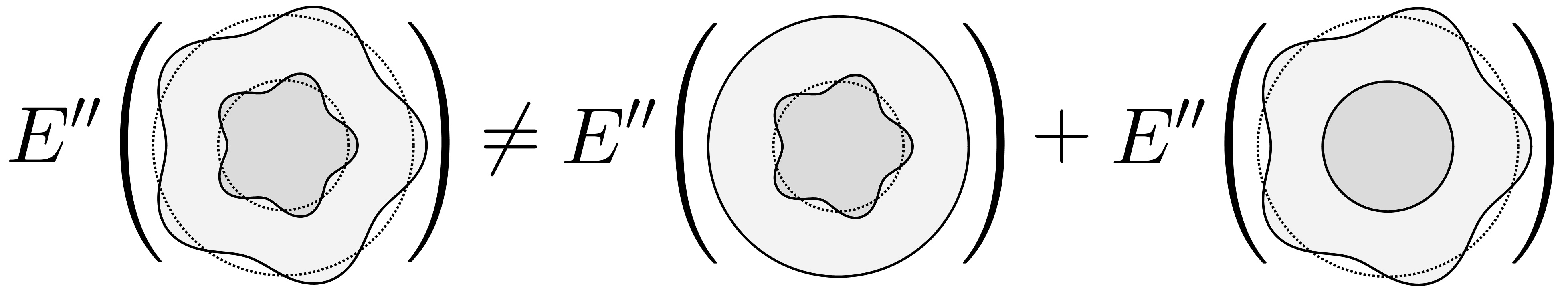
Figure 4: $E^{\prime\prime}$ is nonlinear

In what follows we will assume that the expansion (4.11) holds true for $h_{\pm}$. Combining the result of Theorem 4.7 and the explicit expressions for $u$ and $u^{\prime}=u^{\prime}_{-}+u^{\prime}_{+}$ (given by (1.6) and Proposition 4.5 respectively) yields the following.

$$E^{\prime\prime}(D_{0},\Omega_{0})(\Phi)=\sum_{{k=1}}^{\infty}\sum_{{i=1}}^{d_{k}}\left\{\left(\alpha_{k,i}^{-}\right)^{2}E^{\prime\prime}_{-}(k)+\left(\alpha_{k,i}^{+}\right)^{2}E^{\prime\prime}_{+}(k)+\alpha_{k,i}^{-}\,\alpha_{k,i}^{+}\,E^{\prime\prime}_{\rm res}(k)\right\},$$ (4.18)

where

$$E^{\prime\prime}_{-}(k) =\frac{2R^{N}}{N}\left(\frac{1-\sigma_{c}}{\sigma_{c}}\right)\left(F-k\left(k(1-\sigma_{c})+(N-2+k)(1-\sigma_{c})R^{2-N-2k}\right)\right)\bigg{/}F,$$ (4.19)

$$E^{\prime\prime}_{+}(k) =\frac{2}{N}\left(F-k\left((-N+2-k)(1-\sigma_{c})+(N-2+k+k\sigma_{c})R^{2-N-2k}\right)\right)\bigg{/}F,$$

$$E^{\prime\prime}_{\rm res}(k) =\frac{4(\sigma_{c}-1)R^{1-k}}{N}\left((N-2)k+2k^{2}\right)\bigg{/}F,$$

and $F$ is the term defined at the end of the statement of Proposition 4.5. The term $E^{\prime\prime}_{\rm res}$ will be referred to as the resonant part of $E^{\prime\prime}$. As we can see from (4.18), the resonant part $E^{\prime\prime}_{\rm res}$ arises when the perturbations $h_{-}$ and $h_{+}$ both have a non-zero component corresponding to the same spherical harmonic $Y_{k,i}$.

In this subsection we will consider only the coefficients $k\in\{1,2,\dots\},i\in\{1,\dots d_{k}\}$ such that $\alpha_{k,i}^{-}\,\alpha_{k,i}^{+}=0$ (in other words we will consider only the non-resonant part of $E^{\prime\prime}$). Under this assumption the contributions of $E^{\prime\prime}_{-}(k)$ and $E^{\prime\prime}_{+}(k)$ can be analyzed separately. We have the following result.

Lemma 4.9.

Consider the functions $\mathbb{N}\ni k\mapsto E^{\prime\prime}_{\pm}$. The following holds.

1. The function $k\mapsto E^{\prime\prime}_{-}(k)$ is strictly decreasing for $\sigma_{c}\neq 1$ and constantly zero otherwise.

2. The function $k\mapsto E^{\prime\prime}_{+}(k)$ is strictly decreasing for all $\sigma_{c}>0$.

Proof.

In the following, we will replace the integer parameter $k$ with a real variable $x$ and study the function $x\mapsto E^{\prime\prime}_{\pm}(x)$ in $(0,\infty)$. The calculations are going to be pretty long, although elementary. For the sake of readability we will adopt the following notation:

$$L\mathrel{\mathop{\mathchar 58\relax}}=R^{-1}>1,\quad\lambda\mathrel{\mathop{\mathchar 58\relax}}=\log(L)>0,\quad M\mathrel{\mathop{\mathchar 58\relax}}=N-2\geq 0;\quad P=P(x)\mathrel{\mathop{\mathchar 58\relax}}=L^{2x+M}>1.$$ (4.20)

1. First we will prove the result about $E^{\prime\prime}_{-}$. Rearranging the terms in (4.19) yields:

   $$E_{-}^{\prime\prime}(x)=\frac{2R^{N}}{N}\left(\frac{1-\sigma_{c}}{\sigma_{c}}\right)-\frac{2R^{N}(1-\sigma_{c})^{2}}{N\sigma_{c}}\,\frac{x^{2}+(Mx+x^{2})P}{F}.$$

   We will show that $x\mapsto j(x)\mathrel{\mathop{\mathchar 58\relax}}=\left(x^{2}+(Mx+x^{2})P\right)/F$ is strictly increasing in $(0,\infty)$. To this end we compute the derivative

   $$\frac{d}{dx}j(x)=\frac{MP(MP+2Px+2x)+x^{2}(P+1)^{2}+\sigma_{c}x^{2}P(P-1/P-4x\lambda-2M\lambda)}{F^{2}}.$$

   The denominator in the above is positive and we claim that also the numerator is. To this end it suffices to show that the quantity multiplied by $\sigma_{c}x^{2}P$ in the numerator, namely $P-1/P-4x\lambda-2M\lambda$, is positive for $x\in(0,\infty)$.

   $$\frac{d}{dx}\left(P-\frac{1}{P}-4x\lambda-2M\lambda\right)=2{\lambda}{\left(P+\frac{1}{P}-2\right)}>0\quad\text{for }x>0,$$

   where we used the fact that $L>1$ and that $P\mapsto P+P^{-1}-2$ is a non-negative function vanishing only at $P=1$ (notice that, by definition $P>1$ for positive $x$). We now claim that

   $${\left.\kern-1.2pt\left(P-\frac{1}{P}-4x\lambda-2M\lambda\right)\vphantom{|}\right|_{x=0}}=L^{M}-\frac{1}{L^{M}}-2M\lambda\geq 0.$$

   This can be proven by an analogous reasoning: treating $M$ as a real variable and differentiating with respect to it yield

   $$\frac{d}{dM}\left(L^{M}-\frac{1}{L^{M}}-2M\lambda\right)=\lambda\left(L^{M}+\frac{1}{L^{M}}-2\right)\geq 0$$

   (notice that the equality holds only when $M=0$), moreover,

   $${\left.\kern-1.2pt\left(L^{M}-\frac{1}{L^{M}}-2M\lambda\right)\vphantom{|}\right|_{M=0}}=0,$$

   which proves the claim.

2. Differentiating the expression for $E^{\prime\prime}_{+}(x)$ in (4.19) by $x$ yields the following

   $$\frac{d}{dx}E^{\prime\prime}_{+}(x)=\frac{2\left(a(x)+\sigma_{c}b(x)+\sigma_{c}^{2}x^{2}c(x)\right)}{F^{2}},$$

   where we have set

   $$a(x) \mathrel{\mathop{\mathchar 58\relax}}=x^{2}P^{-1}+M(2x+M)-(x+M)^{2}P-2\lambda(2x^{3}+3Mx^{2}+M^{2}x),$$

   $$b(x) \mathrel{\mathop{\mathchar 58\relax}}=-2x^{2}P^{-1}-M(2x+M)-2(Mx+x^{2})P+2\lambda M(Mx+2x^{2}),$$

   $$c(x) \mathrel{\mathop{\mathchar 58\relax}}=P^{-1}-P+2\lambda(M+2x).$$

   In order to prove claim (ii) of the lemma, it will be sufficient to show that $a(x)<0$, $b(x)<0$ and $c(x)<0$ for all $x>0$.

   We have

   $${\left.\kern-1.2pta(x)\vphantom{|}\right|_{M=0}}=x^{2}\underbrace{(L^{-2x}-L^{2x})}_{<0}-4\lambda x^{3}<0.$$

   Treating now $M$ as a real variable and differentiating yields:

   $$\frac{d}{dM}a(x)=-\lambda x^{2}P^{-1}+2(x+M)\underbrace{(1-L^{M})}_{<0}-\lambda(x+M)^{2}L^{M}-2\lambda(3x^{2}+2Mx)<0.$$

   This implies that $a(x)<0$ for all $x>0$ and all $M\geq 0$.

   As far as $b(x)$ is concerned, we will decompose it further, as follows

   $$b(x)=-2x^{2}P^{-1}-M(2x+M)+2x\,\widetilde{b}(x),$$

   where $\widetilde{b}(x)\mathrel{\mathop{\mathchar 58\relax}}={-(M+x)P+\lambda M(M+2x)}$. We have $\widetilde{b}(0)=M(-L^{M}+\lambda M)$. The quantity $-L^{M}+\lambda M$ is negative for all $M\geq 0$ because it takes the value $-1$ for $M=0$ and is a decreasing function of $M$. As a matter of fact, we have

   $$\frac{d}{dM}(-L^{M}+\lambda M)=-\lambda L^{M}+\lambda=\lambda(-L^{M}+1)<0.$$

   Hence $\widetilde{b}(0)<0$. We claim that $\widetilde{b}(x)$ is also decreasing in $x$, because

   $$\frac{d}{dx}\widetilde{b}(x)=-P-2\lambda(M+x)P+2\lambda M=-P+2\lambda M(-P+1)-2\lambda xP<0.$$

   We conclude that $\widetilde{b}(x)$ (and therefore also $b(x)$) is negative for $x\geq 0$.

   Finally, we show that $c(x)<0$ for $x>0$. We have $c(0)=L^{-M}-L^{M}+2\lambda M$. We claim that this quantity is non-positive for all $M\geq 0$. Indeed

   $${\left.\kern-1.2ptc(0)\vphantom{|}\right|_{M=0}}=0,\quad\text{ and }\quad\frac{d}{dM}c(0)=-\lambda L^{-M}(L^{M}-1)^{2}<0.$$

   Moreover, since

   $$\frac{d}{dx}c(x)=-2\lambda P^{-1}-2\lambda P+4\lambda=-2\lambda(P-1)^{2}<0,$$

   we conclude that also $c(x)<0$ for $x>0$. This implies that the function $x\mapsto E^{\prime\prime}_{+}(x)$ is strictly decreasing in $(0,\infty)$, as claimed.

∎

Moreover, by a simple calculation we can check that

$$E^{\prime\prime}_{\pm}(1)=2(1-\sigma_{c})/F(1)\quad\text{ and }\lim_{k\to\infty}E^{\prime\prime}_{\pm}(k)=-\infty.$$

Now, by combining this observation with Lemma 4.9, we get the behavior of $E^{\prime\prime}_{-}$ and $E^{\prime\prime}_{+}$ (see also Figure 5).

Proposition 4.10 (Behavior of $E^{\prime\prime}_{\pm}$).

1. Let $\sigma_{c}>0$.

2. If $\sigma_{c}>1$, then $E^{\prime\prime}_{\pm}(k)$ is negative for all integer $k\geq 1$.

3. If $\sigma_{c}=1$, then the two functions $E^{\prime\prime}_{-}$ and $E^{\prime\prime}_{+}$ behave differently from one another. Namely, $E^{\prime\prime}_{-}(k)=0$ for all integer $k\geq 1$. On the other hand, $E^{\prime\prime}_{+}(k)>0$ for all integer $k\geq 2$, while $E^{\prime\prime}_{+}(1)=0$.

4. If $0<\sigma_{c}<1$, then $E^{\prime\prime}_{\pm}$ are sign changing. Namely $E^{\prime\prime}_{\pm}(1)>0$, while $E^{\prime\prime}_{\pm}(k)<0$ for large enough $k\in\mathbb{N}$.

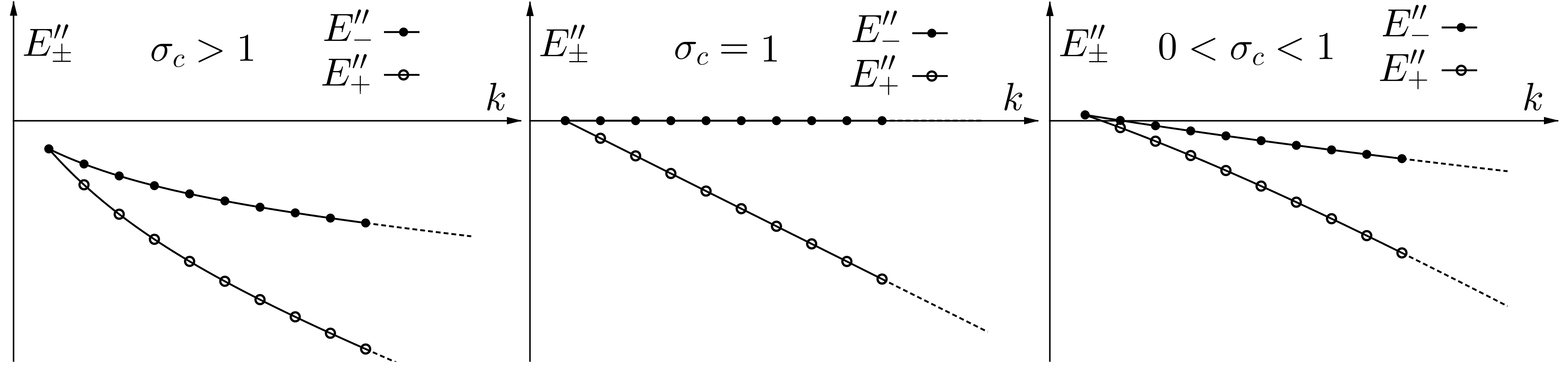
Figure 5: The graphs of $E^{\prime\prime}_{\pm}$ for all possible values of $\sigma_{c}$. Adapted from [Ca2].

4.3.3 Analysis of the resonance effects: proof of Theorem II

Part $(iii)$ of Proposition 4.10 tells us that $E^{\prime\prime}_{\pm}$ changes sign for $0<\sigma_{c}<1$. This means that, by applying Proposition 4.1, we can actually construct perturbations $\Phi_{1}^{\pm},\Phi_{2}^{\pm}\in\mathcal{A}_{\pm}^{*}$ such that $E^{\prime\prime}(D_{0},\Omega_{0})(\Phi_{1}^{\pm})>0$ and $E^{\prime\prime}(D_{0},\Omega_{0})(\Phi_{2}^{\pm})<0$. In other words, we have shown that $(D_{0},\Omega_{0})$ is a saddle shape for the functional $E$ under the volume preserving constraint (indeed, the barycenter preserving condition does not play any role in this).

On the other hand, Proposition 4.10 suggests that the radial configuration $(D_{0},\Omega_{0})$ might be a local maximum for $E$ under the aforementioned constraints. This is actually the case. In order to show it, we will need the following lemma, that takes care of the resonance effects that arise when $\sigma_{c}>1$.

Lemma 4.11.

Suppose that $\boldsymbol{\sigma_{c}>1}$. For any $k\in\{1,2,\dots\}$ and $i\in\{1,\dots,d_{k}\}$ that satisfy $\alpha_{k,i}^{-}\alpha_{k,i}^{+}\neq 0$, we get:

$$\left(\alpha_{k,i}^{-}\right)^{2}E^{\prime\prime}_{-}(k)+\left(\alpha_{k,i}^{+}\right)^{2}E^{\prime\prime}_{+}(k)+\alpha_{k,i}^{-}\alpha_{k,i}^{+}E^{\prime\prime}_{\rm res}(k)\leq 0,$$

where equality holds if and only if $k=1$ (see Figure 6, case V).

Proof.

Since, by hypothesis, $\alpha_{k,i}^{+}\neq 0$, we can put $t\mathrel{\mathop{\mathchar 58\relax}}=\alpha_{k,i}^{-}/\alpha_{k,i}^{+}$. For $k$ fixed, we study the following quadratic polynomial in $t$:

$$Q(t)\mathrel{\mathop{\mathchar 58\relax}}=E^{\prime\prime}_{-}(k)t^{2}+E^{\prime\prime}_{\rm res}(k)t+E^{\prime\prime}_{+}(k).$$

It can be checked that the discriminant of $Q$ is

$$\Delta=\underbrace{\frac{-16(\sigma_{c}-1)(k-1)R^{N}}{\sigma_{c}N^{2}F^{2}}}_{\leq 0}\underbrace{\left(\sigma_{c}k(R^{2-N-2k}-1)+(N-2+k)R^{2-N-2k}+k\right)}_{>0}\cdot G,$$

where we have set $G\mathrel{\mathop{\mathchar 58\relax}}=(\sigma_{c}-1)k(N-1+k)(R^{2-N-2k}-1)+(N-2+2k)R^{2-N-2k}$. We see immediately that $G>0$, as $\sigma_{c}>1$ by hypothesis. We will distinguish two cases. If $k>1$, then $\Delta<0$ and therefore the quadratic polynomial $Q(t)$ has no real roots. Since $Q(0)=E^{\prime\prime}_{+}(k)<0$ (see Proposition 4.10 and Figure 5), then $Q$ must be strictly negative for all other values of $t$ as well. If $k=1$, then $\Delta=0$, which means that $Q(t)$ has one double root (which actually corresponds to $t=1$). We conclude as before. ∎

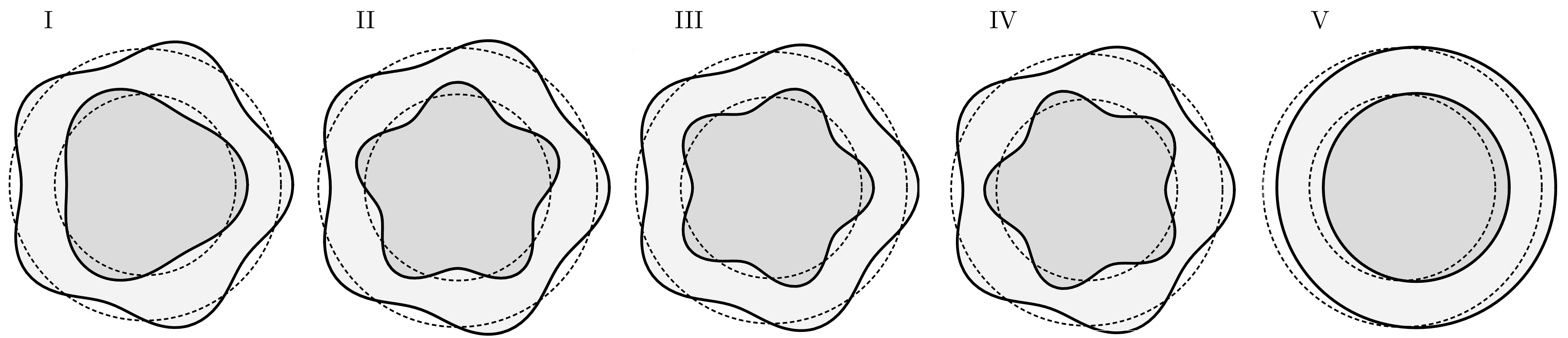
Figure 6: How $(D_{t},\Omega_{t})$ looks like for simple perturbations corresponding to $(h_{-}\cdot n)(R{\boldsymbol{\cdot}})=\alpha Y_{k,i}({\boldsymbol{\cdot}})$ and $h_{+}\cdot n=\beta Y_{m,j}$, for the following values of $k,i,m,j$ and $\alpha,\beta$:
I: $k=3,m=5$. II: $k=m=5$, $i\neq j$. III: $k=m=5$, $i=j$, $\alpha\beta>0$. IV: $k=m=5$, $i=j$, $\alpha\beta<0$. V: $k=m=1$, $i=j$, $\alpha=\beta\neq 0$. Notice that resonance effects appear in cases III, IV and V only. Moreover, as shown in Lemma 4.11, V is the only case when $E^{\prime\prime}(\Phi)=0$ for $\sigma_{c}\neq 1$. Reprinted from [Ca2].

We notice that, for all $\Phi\in\mathcal{A}^{*}$, by (4.3) (see Remark B5) the coefficients $\alpha_{1,i}^{+}$ that appear in the expansion (4.11) must vanish for $i=1,\dots,N$ (in particular, we are able to avoid the case V of Figure 6 by considering $\Phi\in\mathcal{A}^{*}$). Combining this observation with the one at the beginning of this subsection, yields the main result of this chapter.

Theorem 4.12.

If $\sigma_{c}>1$, then $E^{\prime\prime}(D_{0},\Omega_{0})(\Phi)<0$ for all $\Phi\in\mathcal{A}^{*}$. In other words the configuration $(D_{0},\Omega_{0})$ is a local maximum for the functional $E$ under the volume-preserving and barycenter-preserving constraint. If $0<\sigma_{c}<1$, then there exist two perturbation fields $\Phi_{1},\Phi_{2}\in\mathcal{A}^{*}$ such that $E^{\prime\prime}(D_{0},\Omega_{0})(\Phi_{1})>0$ and $E^{\prime\prime}(D_{0},\Omega_{0})(\Phi_{2})<0$. In other words, the configuration $(D_{0},\Omega_{0})$ is a saddle shape for the functional $E$ under the volume and barycenter-preserving constraint. Notice that for $\sigma_{c}=1$ we recover a local version of Pólya’s result Theorem 2.1, namely $E^{\prime\prime}(D_{0},\Omega_{0})(\Phi_{+})<0$ for all $\Phi_{+}\in\mathcal{A}_{+}^{*}$.

Finally, we would like to give some remarks on the results of our computations in the case $k=1$. It corresponds to studying a pair of possibly distinct (volume preserving perturbations that, up to the second order, are indistinguishable from) translations acting on $\partial D_{0}$ and $\partial\Omega_{0}$ simultaneously. We know that the functional $E$ is invariant under rigid motions, i.e. $E(D,\Omega)=E\big{(}T(D),T(\Omega)\big{)}$ for all rigid motions $T\mathrel{\mathop{\mathchar 58\relax}}{{\mathbb{R}}^{N}}\to{{\mathbb{R}}^{N}}$. In turn this implies that for fixed $x_{0}\in{{\mathbb{R}}^{N}}$ and $t\geq 0$:

$$E(D_{0}+tx_{0},\Omega_{0})=E(D_{0},\Omega_{0}-tx_{0})=E(D_{0},\Omega_{0}+tx_{0}).$$

Therefore by differentiating twice with respect to $t$, we get $E^{\prime\prime}_{-}(1)=E^{\prime\prime}_{+}(1)$ (see also Figure 5 on page 5), as we obtained by direct computation right after the proof of Lemma 4.9. Take now two orthogonal directions, say $e_{1}$ and $e_{2}$. We have

$$E(D_{0}+te_{1},\Omega_{0}+te_{2})=E(D_{0}+t(e_{1}-e_{2}),\Omega_{0})=E(D_{0}+\sqrt{2}te_{1},\Omega_{0}),$$ (4.21)

and thus,

$${\left.\kern-1.2pt\frac{d^{2}}{dt^{2}}\vphantom{|}\right|_{t=0}}{E\Big{(}D_{0}+te_{1},\Omega_{0}+te_{2}\Big{)}}=2\,{\left.\kern-1.2pt\frac{d^{2}}{dt^{2}}\vphantom{|}\right|_{t=0}}{E\Big{(}D_{0}+te_{1},\Omega_{0}\Big{)}}=$$ (4.22)

$${\left.\kern-1.2pt\frac{d^{2}}{dt^{2}}\vphantom{|}\right|_{t=0}}{E\Big{(}D_{0}+te_{1},\Omega_{0}\Big{)}}+{\left.\kern-1.2pt\frac{d^{2}}{dt^{2}}\vphantom{|}\right|_{t=0}}{E\Big{(}D_{0},\Omega_{0}+te_{2}\Big{)}},$$

i.e. second order shape derivatives “behave linearly” in this case. On the other hand, if, unlike (4.21), we apply the same translation to both $D_{0}$ and $\Omega_{0}$, then the value of $E$ does not get altered (recall that $E^{\prime\prime}_{\rm res}(1)=-2E^{\prime\prime}_{-}(1)$, see for example (4.19)). Hopefully, this observations might serve as an intuitive explanation of the geometrical meaning of the resonant part $E^{\prime\prime}_{\rm res}$ and the inevitability thereof.

Figure 7: Example of non-resonance (left) and resonance (right) due to the combined effect of two translations.

Chapter 5 A two-phase overdetermined problem of Serrin-type

In this chapter, we will obtain the proof of Theorem III by a perturbation argument. This is one of a series of results about two-phase overdetermined problems that were obtained in [CaMS]. Let $D$, $\Omega\subset{{\mathbb{R}}^{N}}$ be two bounded domains of class $C^{2+\alpha}$ with $\overline{D}\subset\Omega$. We look for a pair $(D,\Omega)$ for which the overdetermined problem (1.8) has a solution for some positive constant $d$. As remarked in Chapter 1, it is sufficient to examine (1.8) with $\sigma_{s}=1$ in the form

$${\mathop{\mathrm{div}}}(\sigma\nabla u)=\beta u-\gamma<0\quad\mbox{ in }\ \Omega,$$ (5.1)

$$u=0\ \quad\qquad\qquad\qquad\qquad\mbox{ on }\partial\Omega,$$ (5.2)

$$\partial_{n}u=-d\ \quad\qquad\qquad\qquad\mbox{ on }\partial\Omega,$$ (5.3)

where $\beta\geq 0$, $\gamma>0$, and $\sigma=\sigma_{c}\chi_{D}+\chi_{\Omega\setminus D}$. By the divergence theorem, the constant $d$ is related to the other data of the problem by the formula:

$$d=\frac{1}{{\rm Per}(\Omega)}\left\{\gamma\,{\rm Vol}(\Omega)-\beta\,\int_{\Omega}u\right\},$$ (5.4)

where, the functionals ${\rm Vol}({\boldsymbol{\cdot}})$ and ${\rm Per}({\boldsymbol{\cdot}})$ have been defined in Example 3.12.

It is obvious that, for all values of $\sigma_{c}>0$, the pair $(B_{R},B_{1})$ is a solution to the overdetermined problem (5.1)–(5.3) for some $d$. We will look for other solution pairs of (5.1)–(5.3) near $(B_{R},B_{1})$ by a perturbation argument which is based on Theorem D, page D.

5.1 Preliminaries

We introduce the functional setting for the proof of Theorem III. As done in Chapter 4, we set $D_{0}\mathrel{\mathop{\mathchar 58\relax}}=B_{R}$ and $\Omega_{0}\mathrel{\mathop{\mathchar 58\relax}}=B_{1}$. For $\alpha\in(0,1)$, let $\phi\in\mathcal{C}^{2+\alpha}({{\mathbb{R}}^{N}},{{\mathbb{R}}^{N}})$ satisfy that $\mathrm{Id}+\phi$ is a diffeomorphism from ${{\mathbb{R}}^{N}}$ to ${{\mathbb{R}}^{N}}$, and

$$\phi=f\,n\ \mbox{ on }\ \partial D_{0},\qquad\phi=g\,n\ \mbox{ on }\ \partial\Omega_{0},$$ (5.5)

where $f$ and $g$ are given functions of class $C^{2+\alpha}$ on $\partial D_{0}$ and $\partial\Omega_{0}$, respectively, and $n$ indistinctly denotes the outward unit normal to both $\partial D_{0}$ and $\partial\Omega_{0}$. Next, we define the sets

$$\Omega_{g}=(\mathrm{Id}+\phi)(\Omega_{0})\ \mbox{ and }\ D_{f}=(\mathrm{Id}+\phi)(D_{0}).$$

If $f$ and $g$ are sufficiently small, $D_{f}$ and $\Omega_{g}$ satisfy $\overline{D_{f}}\subset\Omega_{g}$.

Now, we consider the Banach spaces (equipped with their standard norms, that will be denoted by $\mathinner{\!\left\lVert{\boldsymbol{\cdot}}\right\rVert}$):

$$\mathcal{F}=\left\{f\in C^{2+\alpha}(\partial D_{0})\;\middle|\;\int_{\partial D_{0}}f\,dS=0\right\},\quad{\mathcal{G}}=\left\{g\in C^{2+\alpha}(\partial\Omega_{0})\;\middle|\;\int_{\partial\Omega_{0}}g\,dS=0\right\},$$

$${\mathcal{H}}=\left\{h\in C^{1+\alpha}(\partial\Omega_{0})\;\middle|\;\int_{\partial\Omega_{0}}h\,dS=0\right\}.$$

In order to be able to use Theorem D on page D, we introduce a mapping $\Psi\mathrel{\mathop{\mathchar 58\relax}}\mathcal{F}\times{\mathcal{G}}\to{\mathcal{H}}$ by:

$$\Psi(f,g)=\left\{\left({\nabla}u_{f,g}\cdot n_{g}\right)\circ\left({{\rm Id}}+g\,n\right)+d_{f,g}\right\}J_{\tau}({g})\ \mbox{ for }\ (f,g)\in\mathcal{F}\times{\mathcal{G}}.$$ (5.6)

Here, $u_{f,g}$ is the solution of (5.1)–(5.2) with $\Omega=\Omega_{g}$ and $\sigma=\sigma_{c}\,\chi_{D_{f}}+\chi_{\Omega_{g}\setminus D_{f}}$ and $d_{f,g}$ is computed via (5.4), with $\Omega=\Omega_{g}$ and $u=u_{f,g}$. Also, $n_{g}$ is the outward unit normal to $\partial\Omega_{g}$ (hence we will agree that $n_{g}=n$ for $g\equiv 0$). Finally, the term $J_{\tau}(g)>0$ is the tangential Jacobian associated to the transformation $x\mapsto x+g(x)\,n(x)$ (see (3.12)): this term ensures that the image $\Psi(f,g)$ has zero integral over $\partial\Omega_{0}$ for all $(f,g)\in\mathcal{F}\times{\mathcal{G}}$, as an integration of (5.3) on $\partial\Omega_{g}$ requires, when $d=d_{f,g}$.

Thus, by definition, we have $\Psi(f,g)=0$ if and only if the pair $(D_{f},\Omega_{g})$ solves (5.1)–(5.3). Moreover, we know that the mapping $\Psi$ vanishes at $(f_{0},g_{0})=(0,0)$.

5.2 Computing the derivative of $\Psi$

The first step will consist in proving the Fréchet differentiability of $\Psi$.

Lemma 5.1.

The map $\Psi\mathrel{\mathop{\mathchar 58\relax}}\mathcal{F}\times{\mathcal{G}}\to{\mathcal{H}}$, defined in (5.6) is Fréchet differentiable in a neighborhood of $(0,0)\in\mathcal{F}\times{\mathcal{G}}$.

Proof.

In order to show the differentiability of $\Psi$, we will resort to the machinery developed in Chapter 3. As the elements of $\mathcal{F}$ and ${\mathcal{G}}$ are only defined on the surface of spheres we first need to “extend” them to suitable perturbations in the whole ${{\mathbb{R}}^{N}}$ in order to proceed. To this end consider $\phi\in\mathcal{C}^{2+\alpha}({{\mathbb{R}}^{N}},{{\mathbb{R}}^{N}})$. We can rewrite an analogous formulation of (5.6) for perturbations of the whole ${{\mathbb{R}}^{N}}$:

$$\widehat{\Psi}(\phi)\mathrel{\mathop{\mathchar 58\relax}}={\left.\kern-1.2pt\Big{\{}\left({\nabla}u_{\phi}\cdot n_{\phi}\right)\circ\left({{\rm Id}}+\phi\right)+d_{\phi}\Big{\}}J_{\tau}(\phi)\vphantom{|}\right|_{\partial\Omega_{0}}},$$

where the $\phi$ subscript is used in the natural way, i.e. as in (5.6) according to the notation introduced in (5.5). Moreover, notice that, under (5.5) we have

$$\widehat{\Psi}(\phi)=\Psi(f,g).$$ (5.7)

It is enough to inspection the differentiability of each “piece” of $\widehat{\Psi}$ and then conclude by composition. Put $v_{\phi}\mathrel{\mathop{\mathchar 58\relax}}=u_{\phi}\circ\left({{\rm Id}}+\phi\right)$, we have

$${\nabla}u_{\phi}\circ\left({{\rm Id}}+\phi\right)=\left(I+D\phi\right)^{T}{\nabla}v_{\phi},$$

which is differentiable in a neighborhood of $0$ by Theorem 3.15. The map $\phi\mapsto n_{\phi}\circ\left({{\rm Id}}+\phi\right)$ is differentiable by Proposition 3.6. The function $d_{\phi}$, defined as in (5.4) with the obvious modifications, is also differentiable (its derivative can be computed by the Hadamard formula, see Example 3.12 for the details about ${\rm Per}({\boldsymbol{\cdot}})$ and ${\rm Vol}({\boldsymbol{\cdot}})$). Finally, since $J_{\tau}$ is also differentiable by Lemma 3.7, the proof of the differentiability of $\widehat{\Psi}$ (and thus that of $\Psi$) is complete. ∎

We will now proceed to the actual computation of $\partial_{f}\Psi(0,0)$. Since $\Psi$ is Fréchet differentiable, $\partial_{f}\Psi(0,0)$ can be computed as a Gâteaux derivative:

$$\partial_{f}\Psi(0,0)(f)=\lim_{t\to 0}\frac{\Psi(tf,0)-\Psi(0,0)}{t}\ \mbox{ for }\ f\in\mathcal{F}.$$

From now on, we fix $f\in\mathcal{F}$, set $g=0$ and, to simplify notations, we will write $D_{t},u_{t},d(t)$ in place of $D_{tf},u_{tf,0},d_{tf,0}$. As done previously, we will still write $u$ for $u_{0}$. The following characterization of the shape derivative of $u_{t}$ is a direct consequence of Theorem 3.21.

Lemma 5.2.

For every $f\in\mathcal{F}$, the shape derivative $u^{\prime}$ of $u_{t}$ solves the following:

$$\sigma\Delta u^{\prime}=\beta u^{\prime} \quad\mbox{ in }\ D_{0}\cup(\Omega_{0}\setminus\overline{D_{0}}),$$ (5.8)

$$[\sigma\partial_{n}u^{\prime}]=0 \quad\mbox{ on }\partial D_{0},$$ (5.9)

$$[u^{\prime}]=-[\partial_{n}u]f \quad\mbox{ on }\partial D_{0},$$ (5.10)

$$u^{\prime}=0 \quad\mbox{ on }\ \partial\Omega_{0}.$$ (5.11)

Lemma 5.3.

For all $f\in\mathcal{F}$ we have $d^{\prime}(0)=0$.

Proof.

We rewrite (5.4) as

$$d(t)|\partial\Omega_{0}|-\gamma|\Omega_{0}|=-\beta\int_{\Omega_{0}}u_{t}\,dS,$$

then differentiate and evaluate at $t=0$. The derivative of the left-hand side equals $d^{\prime}(0)\,|\partial\Omega_{0}|$. Thus, we are left to prove that the derivative of the function defined by

$$I(t)=\int_{\Omega_{0}}u_{t}\,dx$$

vanishes at $t=0$.

To this aim, since $u_{t}$ solves (5.1) for $D=D_{t}$, we multiply both sides of this for $u_{t}$ and integrate to obtain that

$$\gamma\,I(t)=\gamma\int_{\Omega_{0}}u_{t}\,dx=\beta\int_{\Omega_{0}}u_{t}^{2}\,dx+\sigma_{c}\int_{D_{t}}\,\mathinner{\!\left\lvert{\nabla}u_{t}\,\right\rvert}^{2}dx+\int_{\Omega_{0}\setminus\overline{D_{t}}}\mathinner{\!\left\lvert{\nabla}u_{t}\,\right\rvert}^{2}dx,$$

after an integration by parts. Thus, the desired derivative can be computed by using the Hadamard formula (Proposition 3.1)

$$\gamma\,I^{\prime}(0) =2\beta\int_{\Omega_{0}}uu^{\prime}+2\int_{\Omega_{0}}\sigma{\nabla}u\cdot{\nabla}u^{\prime}+\int_{\partial D_{0}}[\sigma|\partial_{n}u|^{2}]f$$

$$=2\beta\int_{\Omega_{0}}uu^{\prime}+2\int_{\Omega_{0}}\sigma{\nabla}u\cdot{\nabla}u^{\prime}=0.$$

Here, in the second equality we used that the jump of $\sigma|{\partial_{n}}u|^{2}$ is constant on $\partial D_{0}$ and that $f\in\mathcal{F}$, while, the third equality ensues by integrating (5.8) against $u$. ∎

Theorem 5.4.

The Fréchet derivative $\partial_{f}\Psi(0,0)({\boldsymbol{\cdot}},0)\mathrel{\mathop{\mathchar 58\relax}}\mathcal{F}\to{\mathcal{H}}$ is defined by the formula

$$\partial_{f}\Psi(0,0)(f)=\partial_{n}u^{\prime},$$

where $u^{\prime}$ is the solution of the boundary value problem (5.8)–(5.11).

Proof.

Since $\Psi$ is Fréchet differentiable, we can compute $\partial_{f}\Psi$ as a Gâteaux derivative as follows:

$$\partial_{f}\Psi(0,0)(f)={\left.\kern-1.2pt\frac{d}{dt}\vphantom{|}\right|_{t=0}}\Psi(tf,0)={\left.\kern-1.2pt\frac{d}{dt}\vphantom{|}\right|_{t=0}}\left\{{\nabla}u_{t}(x)\cdot n(x)+d(t)\right\}J_{\tau}(0).$$

Since $J_{\tau}(0)=1$, the thesis is a direct consequence of Lemma 5.3 and definition (3.19). Finally, the fact that this mapping is well-defined (i.e. $\partial_{n}u^{\prime}$ actually belongs to $\mathcal{H}$ for all $f\in\mathcal{F}$) follows from the calculation

$$\int_{\partial\Omega_{0}}\partial_{n}u^{\prime}=\int_{\Omega_{0}}{\mathop{\mathrm{div}}}(\sigma{\nabla}u^{\prime})=\beta\int_{\Omega_{0}}u^{\prime}=\beta\,I^{\prime}(0)=0,$$

where we also used (5.8)–(5.11). ∎

5.3 Applying the implicit function theorem

Here we give the main result of this Chapter, which clearly implies Theorem III.

Theorem 5.5.

There exists $\varepsilon>0$ such that, for all $g\in\mathcal{G}$ with $\mathinner{\!\left\lVert g\right\rVert}<\varepsilon$ there exists a unique $f(g)\in\mathcal{F}$ such that the pair $(D_{f(g)},\Omega_{g})$ is a solution of the overdetermined problem (5.1)–(5.3).

Proof.

This theorem consists of a direct application of Theorem D on page D. We know that the mapping $(f,g)\mapsto\Psi(f,g)$ is Fréchet differentiable and we computed its Fréchet derivative with respect to the variable $f$ in Theorem 5.4. We are left to prove that the mapping $\partial_{f}\Psi(0,0)\mathrel{\mathop{\mathchar 58\relax}}\mathcal{F}\to{\mathcal{H}}$, given in Theorem 5.4, is a bounded and invertible linear transformation.

Linearity and boundedness of $\partial_{f}\Psi(0,0)$ ensue from the properties of problem (5.8)–(5.11).

We are now going to prove the invertibility of $\partial_{f}\Psi(0,0)$. To this end we study the relationship between the spherical harmonic expansions of the functions $f$ and $u^{\prime}$ (see Appendix B for notations and properties of the harmonic functions). Suppose that, for some real coefficients $\alpha_{k,i}$ the following holds

$$f(R\theta)=\sum_{k=1}^{\infty}\sum_{i=1}^{d_{k}}\alpha_{k,i}Y_{k,i}(\theta),\quad\mbox{ for }\theta\in\mathbb{S}^{N-1}.$$ (5.12)

Under the assumption (5.12), we can apply the method of separation of variables to get

$$u^{\prime}(r\theta)=\sum_{k=1}^{\infty}\sum_{i=1}^{d_{k}}\alpha_{k,i}s_{k}(r)Y_{k,i}(\theta),\quad\mbox{ for }r\in(0,R)\cup(R,1)\mbox{ and }\theta\in\mathbb{S}^{N-1}.$$ (5.13)

Here $s_{k}$ denotes the solution of the following problem:

$$\sigma\left\{\partial_{rr}s_{k}+\frac{N-1}{r}\,\partial_{r}s_{k}-\frac{k(k+N-2)}{r^{2}}s_{k}\right\}=\beta s_{k}\,\mbox{ in }(0,R)\cup(R,1),$$ (5.14)

$$s_{k}(R^{+})-s_{k}(R^{-})=\partial_{r}u(R^{-})-\partial_{r}u(R^{+}),\quad\sigma_{c}\,\partial_{r}s_{k}(R^{-})=\partial_{r}s_{k}(R^{+}),$$

$$s_{k}(1)=0,\qquad s_{k}(0)=0,$$

where, by a slight abuse of notation, the letters $\sigma$ and $u$ denote the radial functions $\sigma(|{x}|)$ and $u(|{x}|)$ respectively. Notice that the condition $s_{k}(0)=0$ derives from the fact that $s_{k}$ is non-singular at $r=0$. Indeed, this ensues by multiplying (5.14) by $r^{2}$ and letting $r\to 0$. By (5.13) we see that $\partial_{f}\Psi(0,0)$ preserves the eigenspaces of the Laplace–Beltrami operator, and, in particular, $\partial_{f}\Psi(0,0)$ is invertible if and only if $\partial_{r}s_{k}(1)\neq 0$ for all $k\in\{1,2,\dots\}$. Let us show the latter. Suppose by contradiction that $\partial_{r}s_{k}(1)=0$ for some $k\in\{1,2,\dots\}$. Then, since $s_{k}(1)=0$, by the unique solvability of the Cauchy problem for the ordinary differential equation (5.14), $s_{k}\equiv 0$ on the interval $[R,1]$. Therefore $\partial_{r}s_{k}(R^{+})=0$ and thus also $\partial_{r}s_{k}(R^{-})=0$. Therefore, in view of (5.14), we see that $s_{k}$ achieves neither its positive maximum nor its negative minimum on the interval $[0,R]$. Thus $s_{k}\equiv 0$ also on $[0,R]$. On the other hand, since $\sigma_{c}\neq 1$, we see that $[{\partial_{n}}u]\neq 0$ on $\partial D_{0}$ and hence $s_{k}(R^{-})\not=0$, which is a contradiction. ∎

Lastly, we remark that the volumes of the domains $D_{f(g)}$ and $\Omega_{g}$, found by Theorem 5.5, do not necessarily coincide with those of $D_{0}$ and $\Omega_{0}$ (and the same goes for surface areas). This is because only volume preserving conditions at first order were prescribed in the definitions of $\mathcal{F}$ and ${\mathcal{G}}$. Nevertheless, the arguments of Theorem 5.5 can be refined to gain the control on the domains’ volume (or surface area, for the matter).

Corollary 5.6.

There exists $\varepsilon>0$ such that, for all $\widetilde{g}\in\mathcal{C}^{2+\alpha}(\partial\Omega_{0})$ with $\mathinner{\!\left\lVert\widetilde{g}\right\rVert}<\varepsilon$ and such that ${\rm Vol}(\Omega_{\widetilde{g}})={\rm Vol}(\Omega_{0})$, there exists a unique $\widetilde{f}=\widetilde{f}(\widetilde{g})\in\mathcal{C}^{2+\alpha}(\partial D_{0})$ with ${\rm Vol}(D_{\widetilde{f}})={\rm Vol}(D_{0})$ such that the pair $(D_{\widetilde{f}},\Omega_{\widetilde{g}})$ is a solution of the overdetermined problem (5.1)–(5.3). An analogous result holds true when every occurrence of ${\rm Vol}({\boldsymbol{\cdot}})$ is replaced by ${\rm Per}({\boldsymbol{\cdot}})$ in the statement above.

Proof.

First of all, for any $g\in{\mathcal{G}}$ small enough we will construct a domain $\widetilde{\Omega_{g}}$ such that ${\rm Vol}(\widetilde{\Omega_{g}})={\rm Vol}(\Omega_{0})$. As done in Proposition 4.1, we set $\widetilde{\Omega_{g}}\mathrel{\mathop{\mathchar 58\relax}}=t\Omega_{g}$ for $t=\sqrt[\scriptstyle N]{\frac{\Omega_{0}}{{\rm Vol}{\Omega_{g}}}}$. If $g$ is small enough, then $\widetilde{\Omega_{g}}=\Omega_{\widetilde{g}}$ for some $\widetilde{g}\in\mathcal{C}^{2+\alpha}(\Omega_{0})$. The map $g\mapsto\widetilde{g}$ is continuous in a neighborhood of $g=0$. Moreover, we claim that, for $g$ small enough, the map $g\mapsto\widetilde{g}$ is also invertible. Indeed, by definition $\partial\Omega_{\widetilde{g}}=t\partial\Omega_{g}$ for some $t$ to be determined. We have

$$x+\widetilde{g}(x)n(x)=t\left(x+g(x)n(x)\right)\quad\text{ for all }x\in\partial\Omega_{0}.$$ (5.15)

There is only one value of $t$ such that $g$ in (5.15) has vanishing integral over $\partial\Omega_{0}$. Namely, since $n(x)=x$ on $\partial\Omega_{0}$, we obtain:

$$t=\frac{{\rm Per}(\Omega_{0})+\int_{\partial\Omega_{0}}\widetilde{g}}{{\rm Per}(\Omega_{0})}.$$

Notice that we can make $t$ arbitrarily close to $1$ by controlling the size of $\widetilde{g}$. Of course, the same arguments work for $f\in\mathcal{F}$ as well. We define an auxiliary function $\widetilde{\Psi}(f,g)\mathrel{\mathop{\mathchar 58\relax}}=\Psi(\widetilde{f},\widetilde{g})$, where, by a slight abuse of notation, we used the letter $\Psi$ to denote the extension of (5.6) to $\mathcal{C}^{2+\alpha}(\partial D_{0})\times\mathcal{C}^{2+\alpha}(\partial\Omega_{0})$. As remarked in Proposition 4.1, we have

$${\left.\kern-1.2pt\frac{d}{dt}\vphantom{|}\right|_{t=0}}\widetilde{tf}=f,$$

in other words the perturbations $tf$ and $\widetilde{tf}$ are indistinguishable at first order. Therefore, the statement of Theorem 5.5 holds for the functional $\widetilde{\Psi}$ as well. Hence there exists some $\varepsilon>0$ such that for all $g\in{\mathcal{G}}$ with $\mathinner{\!\left\lVert g\right\rVert}<\varepsilon$, there exists a unique $f=f(g)\in\mathcal{F}$ such that $\widetilde{\Psi}(f,g)=\Psi(\widetilde{f},\widetilde{g})$. Up to choosing a smaller $\varepsilon>0$, we can conclude by the invertibility of the map $\widetilde{{\boldsymbol{\cdot}}}$. ∎

Appendix A Elements of tangential calculus

Let $\omega$ be a bounded open set of class $\mathcal{C}^{1}$. For every $g\in\mathcal{C}^{1}(\partial\omega)$ we define its tangential gradient as

$${{{\nabla}}_{\tau}}g\mathrel{\mathop{\mathchar 58\relax}}={\nabla}\widetilde{g}-({\nabla}\widetilde{g}\cdot n)n\quad\text{ on }\partial\omega,$$ (A.1)

where $\widetilde{g}$ is an extension of class $\mathcal{C}^{1}$ of $g$ to a neighborhood of $\partial\omega$. Notice that, by density, the tangential gradient can be defined in the natural way for all functions $g\in W^{1,1}(\partial\omega)$. It is easy to see that this definition does not depend on the choice of the extension. Indeed, this is equivalent to showing that ${\nabla}\widetilde{g}=({\nabla}\widetilde{g}\cdot n)n$ on $\partial\omega$ for all $\widetilde{g}$ of class $\mathcal{C}^{1}$ on a neighborhood of $\partial\omega$ with $\widetilde{g}\equiv 0$ on $\partial\omega$. To this end, fix a point $x_{0}\in\partial\omega$ and take a smooth path $\gamma\mathrel{\mathop{\mathchar 58\relax}}[0,1]\to\partial\omega$ with $\gamma(0)=x_{0}$. Since, by assumption, $\widetilde{g}(\gamma(t))=0$ for all $t$, we have ${\nabla}\widetilde{g}(x_{0})\cdot\gamma^{\prime}(0)=0$. By the arbitrariness of $x_{0}$ and $\gamma$ we conclude that ${\nabla}\widetilde{g}$ is parallel to $n$ at each point of $\partial\omega$, which was our claim. One obvious property of the tangential gradient is the following:

$${{{\nabla}}_{\tau}}g\cdot n=0\quad\text{ for all }g\in\mathcal{C}^{1}(\partial\omega).$$ (A.2)

Let $w\in\mathcal{C}^{1}(\partial\omega,{{\mathbb{R}}^{N}})$. The tangential divergence of $w$ is defined as

$${\mathop{\mathrm{div}}}_{\tau}w\mathrel{\mathop{\mathchar 58\relax}}={\mathop{\mathrm{div}}}\widetilde{w}-n\cdot\left(D\widetilde{w}\,n\right),$$ (A.3)

where $\widetilde{w}$ is a $\mathcal{C}^{1}$ extension of $w$ to a neighborhood of $\partial\omega$. This definition can by extended by density to vector fields $w\in W^{1,1}(\partial\omega,{{\mathbb{R}}^{N}})$. Just like the tangential gradient, the definition of tangential divergence is independent of the extension chosen. Indeed one can verify that

$${\mathop{\mathrm{div}}}\widetilde{w}-n\cdot\left(D\widetilde{w}n\right)=\mathop{\mathrm{tr}}(D_{\tau}w),$$ (A.4)

where

$$D_{\tau}w\text{ is the matrix whose $i$-th row is given by }{{{\nabla}}_{\tau}}w_{i}.$$ (A.5)

The following tangential versions of the Leibniz rule hold true: for all $f,g\in\mathcal{C}^{1}(\partial\omega)$ and $w\in\mathcal{C}^{1}(\partial\omega,{{\mathbb{R}}^{N}})\mathrel{\mathop{\mathchar 58\relax}}$

$${{{\nabla}}_{\tau}}(fg)=f{{{\nabla}}_{\tau}}g+g{{{\nabla}}_{\tau}}f,\qquad{\mathop{\mathrm{div}}}_{\tau}(gw)=g\,{\mathop{\mathrm{div}}}_{\tau}w+w\cdot{{{\nabla}}_{\tau}}g.$$ (A.6)

The first identity above follows directly from the definition of tangential gradient (A.1), while the second identity can be proved by applying the first one to each row of $D_{\tau}(gw)$ and then taking the trace (recall (A.4)). Tangential divergence is used to define the (additive) mean curvature $H$ (i.e. the sum of the principal curvatures) of a surface by means of the unit normal $n$:

$$H\mathrel{\mathop{\mathchar 58\relax}}={\mathop{\mathrm{div}}}_{\tau}n.$$ (A.7)

Actually, if $\omega$ is an open set of class $\mathcal{C}^{2}$, then ${\mathop{\mathrm{div}}}\,\widetilde{n}=H$ on $\partial\omega$ for all unitary extensions $\widetilde{n}$ of class $\mathcal{C}^{1}$ of the outward unit normal $n$. Indeed $(D\widetilde{n})\widetilde{n}=0$ on $\partial\omega$ because the norm of $\widetilde{n}$ is constant in a neighborhood of $\partial\omega$. Therefore ${\mathop{\mathrm{div}}}\widetilde{n}={\mathop{\mathrm{div}}}_{\tau}n=H$.

Now, let $w_{\tau}$ denote the tangential part of a vector field $w$ on $\partial\omega$, that is

$$w_{\tau}\mathrel{\mathop{\mathchar 58\relax}}=w-(w\cdot n)n\quad\text{ on }\partial\omega.$$ (A.8)

Let $\omega$ of class $\mathcal{C}^{2}$ and $w\in W^{1,1}(\partial\omega,{{\mathbb{R}}^{N}})$. By combining (A.8), (A.6), (A.2) and (A.7), we get the following decomposition result for the tangential divergence.

$${\mathop{\mathrm{div}}}_{\tau}w={\mathop{\mathrm{div}}}_{\tau}w_{\tau}+Hw\cdot n\quad\text{ on }\partial\omega.$$ (A.9)

Lemma A1 (Tangential Stokes formula).

Let $\omega$ be a bounded open set of class $\mathcal{C}^{2}$ and $w\in W^{1,1}(\partial\omega,{{\mathbb{R}}^{N}})$. Then

$$\int_{\partial\omega}{\mathop{\mathrm{div}}}_{\tau}w=\int_{\partial\omega}Hw\cdot n.$$

Proof.

We would like to follow along the same lines as [DZ, Chapter 8, Subsection 5.5, page 367], where an elegant proof is given using shape derivatives. By density we might assume, without loss of generality, that $w\in\mathcal{C}^{1}(\partial\omega,{{\mathbb{R}}^{N}})$. Moreover, in what follows the same notation $w$ will denote a $\mathcal{C}^{1}$ extension of $w$ to the whole ${{\mathbb{R}}^{N}}$. Take now an Hadamard perturbation $\Phi(t)=t\xi n$ on $\partial\omega$. By the divergence theorem applied to the perturbed domain $\omega_{t}$, we have

$$\int_{\omega_{t}}{\mathop{\mathrm{div}}}w=\int_{\partial\omega_{t}}w\cdot n_{t},\quad\text{ for }t\geq 0\text{ small},$$ (A.10)

where $n_{t}$ is taken to be unitary. Differentiating both sides with the aid of the usual and surface Hadamard formulas (Proposition 3.1 and Corollary 3.4) and Proposition 3.6 yields

$$\int_{\partial\omega}{\mathop{\mathrm{div}}}w\,\xi=\int_{\partial\omega}-w\cdot{{{\nabla}}_{\tau}}\xi+{\partial_{n}}(w\cdot n)\xi+Hw\cdot n\xi.$$

Suppose $\xi\equiv 1$ on $\partial\omega$. We get

$$\int_{\partial\omega}{\mathop{\mathrm{div}}}w=\int_{\partial\omega}{\partial_{n}}(w\cdot n)+\int_{\partial\omega}Hw\cdot n.$$

Since ${\partial_{n}}(w\cdot n)=n\cdot(Dw\,n)$ the thesis follows by the definition of tangential divergence (A.3). ∎

Combining Lemma A1 and the second identity of (A.6) yields

$$\int_{\partial\omega}w\cdot{{{\nabla}}_{\tau}}g=-\int_{\partial\omega}g\,{\mathop{\mathrm{div}}}_{\tau}w+\int_{\partial\omega}Hgw\cdot n.$$ (A.11)

We will now introduce the last tangential differential operator of this appendix: the Laplace–Beltrami operator. For $\omega$ of class $\mathcal{C}^{2}$, the Laplace–Beltrami operator, denoted by $\Delta_{\tau}$, is defined as

$$\Delta_{\tau}u={\mathop{\mathrm{div}}}_{\tau}({{{\nabla}}_{\tau}}u)\quad\text{ for }u\in W^{2,1}(\partial\omega).$$ (A.12)

Proposition A2 (Decomposition of the Laplace operator).

Assume that $\omega$ is an open set of class $\mathcal{C}^{2}$ and let $u\in\mathcal{C}^{2}(\overline{\omega})$, then

$$\Delta u=\partial_{nn}u+H{\partial_{n}}u+\Delta_{\tau}u\quad\text{ on }\partial\omega,$$ (A.13)

where $\partial_{nn}u\mathrel{\mathop{\mathchar 58\relax}}=n\cdot(D^{2}u\,n)$. Notice that, by density, (A.13) can remains true for functions $u\in H^{3}(\omega)$.

Proof.

By definition of tangential divergence we have

$$\Delta u={\mathop{\mathrm{div}}}({\nabla}u)={\mathop{\mathrm{div}}}_{\tau}({\nabla}u)+n\cdot(D({\nabla}u)n)\quad\text{ on }\partial\omega.$$

We conclude noticing that, by (A.9),

$${\mathop{\mathrm{div}}}_{\tau}({\nabla}u)={\mathop{\mathrm{div}}}_{\tau}({{{\nabla}}_{\tau}}u)+H{\partial_{n}}u=\Delta_{\tau}u+H{\partial_{n}}u.$$

∎

We conclude by stating a corollary of Lemma A1:

Proposition A3 (Tangential integration by parts).

Assume that $\omega$ is a bounded open set of class $\mathcal{C}^{2}$. For $f\in H^{2}(\omega)$ and $g\in H^{3}(\omega)$ the following holds

$$\int_{\partial\omega}{{{\nabla}}_{\tau}}f\cdot{{{\nabla}}_{\tau}}g=-\int_{\partial\omega}f\Delta_{\tau}g.$$

Notice that the formula above bears a striking resemblance to the usual integration by parts formula on open sets, and the absence of the “boundary term” is due to the fact that $\partial\omega$ has no boundary.

Appendix B Spherical harmonics

For integer $N\geq 2$ and $k\geq 0$, let $\mathbb{P}_{k}(\mathbb{R}^{N})$ denote the set of all polynomial functions ${{\mathbb{R}}^{N}}\to\mathbb{R}$ whose degree is at most $k$. Moreover, let $\mathbb{H}_{k}({{\mathbb{R}}^{N}})$ denote the set of harmonic polynomials in $\mathbb{P}_{k}({{\mathbb{R}}^{N}})$. Lastly, let $\mathbb{Y}_{k}({{\mathbb{R}}^{N}})$ denote the subset of polynomials in $\mathbb{H}_{k}({{\mathbb{R}}^{N}})$ that are also harmonic. $\mathbb{Y}_{k}({{\mathbb{R}}^{N}})$ is a vector space over the reals; its dimension is finite and will be denoted by $d_{k}$. A combinatoric argument shows that

$$d_{0}=1,\quad\quad d_{k}=\frac{(2k+N-2)(k+N-3)}{k!(N-2)!}\quad\text{ for }k\geq 1.$$ (B.1)

We will now introduce the so-called harmonic decomposition of a polynomial, it will be a key ingredient in proving Theorem B3. We refer to [SW, Theorem 2.1, Chapter IV] for a proof.

Lemma B1 (Harmonic decomposition).

Every polynomial $p\in\mathbb{P}_{k}({{\mathbb{R}}^{N}})$ can be uniquely written in the form

$$p=h_{k}+|x|^{2}h_{k-2}+\dots+|x|^{2m}h_{k-2m},$$

where $m=\left[k/2\right]$ and $h_{i}\in\mathbb{H}_{i}({{\mathbb{R}}^{N}})$ for each $i$.

Let $\mathbb{Y}_{k}(\SS^{N-1})\mathrel{\mathop{\mathchar 58\relax}}=\left\{{\left.\kern-1.2pth\vphantom{|}\right|_{\SS^{N-1}}}\;\middle|\;h\in\mathbb{Y}_{k}({{\mathbb{R}}^{N}})\right\}$. Elements of $\mathbb{Y}_{k-1}(\SS^{N-1})$ are usually called spherical harmonics of degree $k$ in the literature. Notice that every homogeneous polynomial $p$ of degree $k$ is uniquely determined by its restriction to $\SS^{N-1}$ by means of the relation

$$p(x)=|x|^{k}{\left.\kern-1.2ptp\vphantom{|}\right|_{\SS^{N-1}}}(x/|x|)\quad\text{ for }x\neq 0.$$ (B.2)

Therefore, we have

$$\dim\mathbb{Y}_{k}(\SS^{N-1})=\dim\mathbb{Y}_{k}({{\mathbb{R}}^{N}})=d_{k}.$$

Let now $\{Y_{k,i}\}_{i=1}^{d_{k}}$ denote an orthonormal basis of $\mathbb{Y}_{k}(\SS^{N-1})$. Another simple consequence of (B.2) is the following.

Proposition B2.

Spherical harmonics $Y_{k}\in\mathbb{Y}_{k}(\SS^{N-1})$ solve to the following eigenvalue problem on the unit sphere:

$$-\Delta_{\tau}Y_{k}=\lambda_{k}Y_{k}\;\text{ on }\SS^{N-1},\quad\text{ where }\;\lambda_{k}=k(k+N-2).$$ (B.3)

In particular, spherical harmonics of distinct degree are mutually orthogonal in $L^{2}(\SS^{N-1})$.

Proof.

Take an arbitrary $Y_{k}\in\mathbb{Y}_{k}(\SS^{N-1})$. By (B.2) we know that the extension $H_{k}(x)\mathrel{\mathop{\mathchar 58\relax}}=|x|^{k}Y_{k}(x/|x|)$ is a harmonic function. Therefore, by Proposition A2 we can write

$$0=\Delta H_{k}=k(k-1)Y_{k}+(N-1)kY_{k}+\Delta_{\tau}Y_{k}\quad\text{ on }\SS^{N-1}.$$

Rearranging the terms yields $-\Delta_{\tau}Y_{k}=k(k+N-2)Y_{k}$ on ${\SS^{N-1}}$. Orthogonality will be proved in a classical way. Let $Y_{j}\in\mathbb{Y}_{j}(\SS^{N-1})$ and $Y_{k}\in\mathbb{Y}_{k}(\SS^{N-1})$ be two spherical harmonics corresponding to different indices $j\neq k$. By tangential integration by parts (Proposition A3), we have

$$\int_{\SS^{N-1}}{{{\nabla}}_{\tau}}Y_{j}\cdot{{{\nabla}}_{\tau}}Y_{k}=-\int_{\SS^{N-1}}Y_{k}\Delta_{\tau}Y_{j}=\lambda_{j}\int_{\SS^{N-1}}Y_{j}Y_{k}.$$

Inverting the roles of $Y_{j}$ and $Y_{k}$ we get $\int_{\SS^{N-1}}{{{\nabla}}_{\tau}}Y_{j}\cdot{{{\nabla}}_{\tau}}Y_{k}=\lambda_{k}\int_{\SS^{N-1}}Y_{j}Y_{k}$. Since, by assumption, $\lambda_{j}\neq\lambda_{k}$, then $\int_{\SS^{N-1}}Y_{j}Y_{k}$ must vanish. ∎

We have the following result.

Theorem B3.

The spherical harmonics $\{Y_{k,i}\}$ (where $k\in\{0,1,\dots\}$ and $i\in\{1,\dots,d_{k}\}$ for every $k$) form a complete orthonormal system in $L^{2}(\SS^{N-1})$.

Proof.

Orthonormality is clear. We will now prove completeness. By invoking the density of $\mathcal{C}(\SS^{N-1})$ in $L^{2}(\SS^{N-1})$, it will be enough to show that

$$\mathcal{C}(\SS^{N-1})=\bigoplus_{k\geq 0}\mathbb{Y}_{k}(\SS^{N-1}).$$

Now, by Stone-Weierstrass approximation theorem (see [Bre, Theorem 2.2, page 36]), we know that for every compact set $K\subset{{\mathbb{R}}^{N}}$, continuous functions on $K$ can be approximated by polynomials in the max-norm with arbitrary precision. Finally, since every harmonic polynomial can be written as the sum of homogeneous harmonic polynomials, we conclude by Lemma B1. ∎

Remark B4.

In particular, Theorem B3 ensures that every solution of (B.3) can be written as the restriction to the unit sphere of some homogeneous harmonic polynomial.

Theorem B3 can be applied in the computations regarding perturbations of the ball. For instance, let $\Phi=th$ be an Hadamard perturbation acting on the unit ball $B_{1}$. Then, spherical harmonics form the “right” basis to work with. The function $h\cdot n\mathrel{\mathop{\mathchar 58\relax}}{\SS^{N-1}}\to\mathbb{R}$ can be decomposed as $\sum_{k,i}\alpha_{k,i}Y_{k,i}$ for $\{\alpha_{k,i}\}_{k,i}\subset\mathbb{R}$. This allows us to study the Hadamard perturbations generated by each spherical harmonic in the basis one by one and then recover the general case by (bi)linearity.

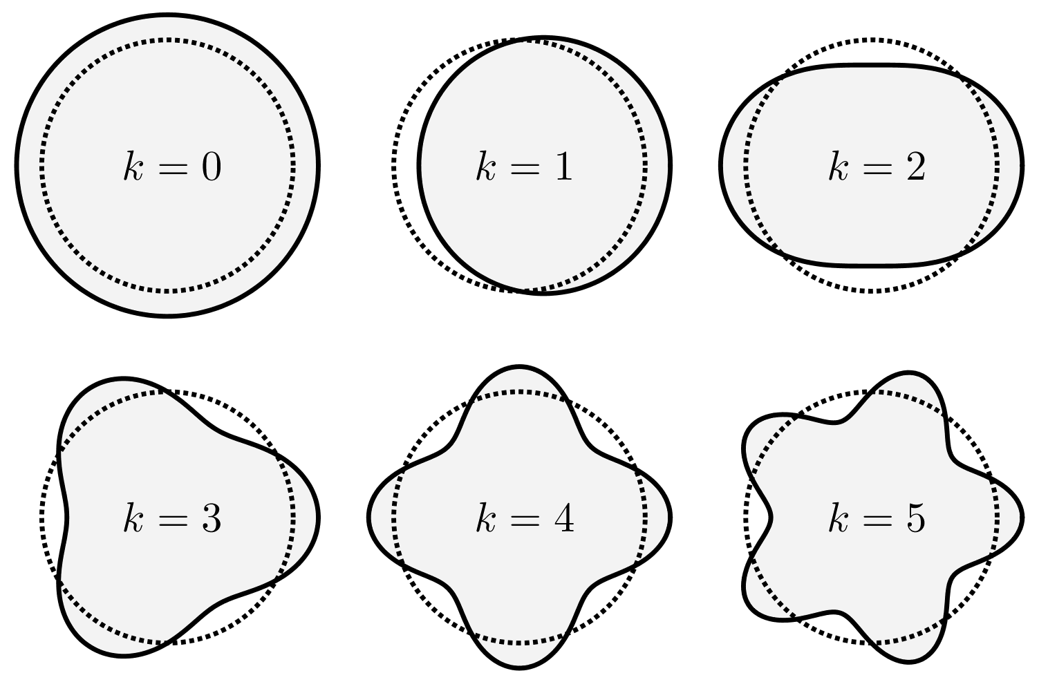
Figure 8: How perturbations of the unit ball generated by spherical harmonics of various degree look (in two dimensions).

Remark B5.

A particular advantage brought by this approach is the following: geometrical constraints often assume an elegant form when rephrased using spherical harmonics. As a matter of fact (see Figure 8), Hadamard perturbations generated by spherical harmonics of degree $k\geq 0$ satisfy the first order volume preserving condition (4.1) for all $k\neq 0$, while the first order barycenter preserving condition (4.3) is satisfied for all $k\neq 1$. The statement above follows immediately from the orthogonality relations among spherical harmonics proved in Proposition B2.

Bibliography

- [Ad] R.A. Adams. Sobolev Spaces. Academic Press, New York, London (1975).
- [Al] A.D. Alexandrov. Uniqueness theorem for surfaces in the large.V. Vestnik, Leningrad Univ. 13.19 (1958): 5–8, Amer. Math. Soc. Transl. 21.2: 412–416.
- [AB] L. Ambrosio, G. Buttazzo. An optimal design problem with perimeter penalization. Calc. Var. Part. Diff. Eq. 1 (1993): 55–69.
- [AS] C. Athanasiadis, I.G. Stratis. On some elliptic transmission problems. Annales Polonici Mathematici 63.2 (1996): 137-154.
- [Bra] L. Brasco. On torsional rigidity and principal frequencies: an invitation to the Kohler-Jobin rearrangement technique. ESAIM: Control, Optimisation and Calculus of Variations, 20.2 (2014): 315–338.
- [Bre] A. Bressan. Lecture Notes on Functional Analysis and Linear PDEs. Available at http://www.math.psu.edu/bressan/.
- [Bu] A. Burchard. A Short Course on Rearrangement Inequalities. Available at http://www.math.utoronto.ca/almut/rearrange.pdf.
- [CDKT] F. Caubet, M. Dambrine, D. Kateb, C.Z. Timimoun.A Kohn-Vogelius formulation to detect an obstacle immersed in a fluid. Inverse Problems and Imaging 7.1 (2013): 123–157.
- [Ca1] L. Cavallina. Locally optimal configurations for the two-phase torsion problem in the ball. Nonlinear Anal. 162 (2017): 33–48.
- [Ca2] L. Cavallina. Stability analysis of the two-phase torsional rigidity near a radial configuration. Published online in Applicable Analysis. Available at https://www.tandfonline.com/doi/full/10.1080/00036811.2018.1478082
- [CaMS] L. Cavallina, R. Magnanini, S. Sakaguchi. Two-phase heat conductors with a surface of the constant flow property. Submitted for publication.
- [CZ] Z. Chen, J. Zou. Finite element methods and their convergence for elliptic and parabolic interface problems. Num. Math. 79.2 (Apr 1998): 175–202
- [CoMS] C. Conca, R. Mahadevan, L. Sanz. Shape derivative for a two-phase eigenvalue problem and optimal configuration in a ball. In CANUM 2008, ESAIM Proceedings 27, EDP Sci., Les Ulis, France (2009): 311–321.
- [DK] M. Dambrine, D. Kateb. On the shape sensitivity of the first Dirichlet eigenvalue for two-phase problems. Applied Mathematics and Optimization 63.1 (Feb 2011): 45–74.
- [DL] M. Dambrine, J. Lamboley. Stability in shape optimization with second variation. arXiv:1410.2586v1 [math.OC] (9 Oct 2014).
- [DZ] M.C. Delfour, Z.P. Zolésio. Shapes and Geometries: Analysis, Differential Calculus, and Optimization. SIAM, Philadelphia (2001).
- [ERS] J. Elschner, J. Rehberg, G. Schmidt. Optimal regularity for elliptic transmission problems including interfaces. Interface and Free Boundaries 9 (2007): 233–252.
- [GT] D. Gilbarg, N.S. Trudinger. Elliptic Partial Differential Equation of Second Order, second edition. Springer.
- [Ha] J. Hadamard. Mémoire sur le problème d’analyse relatif à l’équilibre des plaques élastiques encastrées (1907), from Oevres de J. Hadamard, CNRS Paris 1968.
- [HP] A. Henrot, M. Pierre. Variation et optimisation de formes. Mathématiques & Applications. Springer Verlag, Berlin (2005).
- [HL] R. Hiptmair, J. Li. Shape derivatives in differential forms I: an intrinsic perspective, Ann. Mate. Pura Appl. 192.6 (2013): 1077–1098.
- [Lar] C.J. Larsen. Regularity of components in optimal design problems with perimeter penalization, Calc. Var. Part. Diff. Eq. 16 (2003): 17–29.
- [Li] F.H. Lin. Variational problems with free interfaces. Calc. Var. Part. Diff. Eq. 1 (1993): 149–168.
- [Ma] R. Magnanini. Alexandrov, Serrin, Weinberger, Reilly: symmetry and stability by integral identities. Bruno Pini Mathematical Analysis Seminar (2017): 121–141.
- [Ni] L. Nirenberg. Topics in Nonlinear Functional Analysis, Revised reprint of the 1974 original. Courant Lecture Notes in Mathematics, 6, American Mathematical Society, Providence, RI (2001).
- [NT] C. Nitsch, C. Trombetti. The classical overdetermined Serrin problem. Complex Variables and Elliptic Equations 63.7–8 (2018): 1107–1122.
- [NP] A. Novruzi, M. Pierre. Structure of shape derivatives. Journal of Evolution Equations 2 (2002): 365–382.
- [Po] G. Pólya. Torsional rigidity, principal frequency, electrostatic capacity and symmetrization. Q. Appl. Math. 6 (1948): 267–277.
- [Se] J. Serrin. A symmetry problem in potential theory. Arch. Rat. Mech. Anal., 43 (1971): 304–318.
- [Si] J. Simon. Second variations for domain optimization problems, International Series of Numerical Mathematics, vol. 91. Birkhauser, Basel (1989): 361–378.
- [SW] E.M. Stein, G. Weiss. Fourier Analysis on Euclidean Spaces, Princeton University Press (1971).
- [XB] J. Xiong, J. Bao. Sharp Regularity for Elliptic Systems Associated with Transmission Problems. Potential Anal 39 (2013): 169–194.