Segmenting the Future

Abstract

Predicting the future is an important aspect for decision-making in robotics or autonomous driving systems, which heavily rely upon visual scene understanding. While prior work attempts to predict future video pixels, anticipate activities or forecast future scene semantic segments from segmentation of the preceding frames, methods that predict future semantic segmentation solely from the previous frame RGB data in a single end-to-end trainable model do not exist. In this paper, we propose a temporal encoder-decoder network architecture that encodes RGB frames from the past and decodes the future semantic segmentation. The network is coupled with a new knowledge distillation training framework specific for the forecasting task. Our method, only seeing preceding video frames, implicitly models the scene segments while simultaneously accounting for the object dynamics to infer the future scene semantic segments. Our results on Cityscapes and Apolloscape outperform the baseline and current state-of-the-art methods. Code is available at https://github.com/eddyhkchiu/segmenting_the_future/.

1 Introduction

Prediction of dynamics in visual scenes is one of the crucial components of intelligent decision-making in robotics and autonomous driving applications [40, 10, 9]. To this end, learning useful representations that enable reasoning about the future has recently been of great attention. Example applications are anticipating activities [34], predicting visual context [37], tracking to the future [1], forecasting human dynamics [4], tracking dynamics in scenes [23, 22], and predicting instance segments [22].

In recent years, semantic and instance segmentation of videos [21, 6, 20, 39] have become the leading methods to transform the scene into its semantic components, such as street, tree, vehicles, pedestrians, and obstacles. These semantic entities provide a high-level interpretation of the scene and hence predicting them can be of great interest. We argue that prediction of pixels in the RGB space is an overly perplexing task, while predicting high-level scene properties is sufficient, can be more useful, and is easier to interpret for decision-making purposes. Towards this direction, previous work predicted future semantic segments given the segmentation of the preceding frames [28, 23], or more sparsely predicted future instance segmentation from previous frames [22]. In contrast, we (1) do not require segmentation of previous frames and (2) provide a dense forecast for all regions in the frame.

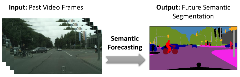
Figure 1: We obtain future semantic segmentation directly from preceding past frames in a single end-to-end trainable model. Our method implicitly infers the scene semantic segments while also forecasting the future configuration.

In this paper, we propose a model that predicts the future semantic segmentation in a video directly from pure RGB data of the previous frames (see Fig. 1). Inspired by the success of multi-resolution fully convolutional networks (FCN) [21, 6, 20, 31] segmentation, we propose an architecture that takes in a temporal sequence of frames and outputs the future semantic segmentation map. Unlike previous work [37, 16, 26] that attempted to predict future RGB video frames from preceding frames, our approach provides future semantic maps, which can enable reasoning about the forthcoming events. Alternatively, [23] adopted a two-stage approach, first using the past RGB sequences to predict the future RGB frame, and then generating the future segmentation on top of that. On the contrary, one of our key observations is that future frame pixel values are not necessary for generating future semantic segmentations, which is itself an easier task than generating future pixel values. We propose a single stage end-to-end trainable model that learns to implicitly model the scene segments, and simultaneously account for the intrinsic dynamics of semantic maps for several object categories to predict future segmentation. In particular, this is a challenging task as objects in the semantic maps can significantly deform over the video frames due to changes in camera viewpoint, illumination, or orientation. To alleviate these challenges, our architecture encodes the sequence of input frames in a multi-resolution manner into a collective latent representation, and then decodes this representation gradually to the future semantic map. We propose a novel knowledge distillation training framework that extracts future information to further refine the future semantic map. During the training stage, we utilize a fixed pre-trained single frame segmentation model and use it as a ‘teacher network.’ Taking the future frame as the input, it predicts the future segmentation. The predicted output from the teacher network provides additional information to guide the training of our main forecasting model, denoted by ‘student network.’ This introduces one more training loss component, called distillation loss, which measures the difference between the outputs of the teacher and student networks. During inference, the teacher network is not used and the student network itself forecasts the future semantic segmentation using only the past RGB sequence as the input. With this new distillation training framework, we can further improve the forecasting performance.

To evaluate the performance of our method, we use the Cityscapes [5] and the Apolloscape [13] datasets under several scenarios, and compare our results with baseline methods. We predict the future semantic segmentation maps at three different temporal horizons (i.e., , short-term, mid-term, and long-term) from the preceding RGB frames. Our method outperforms the previous methods although solving a much harder problem of predicting all semantic segments by only using past raw image sequences as input. Not only we define this harder problem and achieve the state-of-the-art, but we also outperform prior works under the simpler task that uses past semantic segmentation to forecast the future, even without modifying any part of our model.

In summary, our contributions are three-fold. First, we propose a single-stage end-to-end trainable model for the challenging task of predicting future semantic segmentation based on only the preceding RGB frames. Second, we propose a new knowledge distillation training framework that better uses future information. We introduce an additional distillation loss using a teacher network during training. We show that our method can uncover the relations between the previous and future frames while taking the motion into account. Third, our proposed model also outperforms the previous state-of-the-art methods on the simpler setting that uses past semantic segmentation to forecast the future.

2 Related Work

Semantic and Instance Segmentation: Semantic segmentation problems are often modeled by fully convolutional architectures (FCN) with multiple scales [21, 6, 20, 31, 26], or by larger receptive fields [41]. On the other hand, instance segmentation often maintains an strategy to generate instance-proposal regions [30] as part of the segmentation pipeline. Some early methods for this task integrate object detection and segmentation sequentially [36, 27], and more recently in a joint multi-task end-to-end framework [19].

Other works have explored the utilization of temporal information and consistency across frames. Some of them are based on 3D data structures and operations [38] or CRF models [18], and others leveraged optical flow [3]. More recently, a number of methods utilize predictive feature learning techniques to enhance video segmentation. For instance, [14] built a predictive model to learn features from the preceding input frames. All these works segment the last seen frame and do not evaluate the predictive power of the learned features for segmenting the future.

Video Forecasting: Visual forecasting tasks were defined as extrapolating video pixels to create realistic future frames [26, 37, 2]. Although these methods have some success in predicting the future at the pixel-level, modeling raw RGB pixel values is rather cumbersome in comparison with predicting future high-level properties of the video. These high-level properties can not only be sufficient for analysis in many applications but also be more beneficial due to the higher level of semantic abstraction. Examples are anticipation of activities [34, 17] or trajectories [1].

One of the best procedures for understanding and parsing scenes is scene semantic segmentation [38]. Recently, a few works proposed techniques for predicting semantic segmentation in videos. For instance, [23] defined future semantic segmentation prediction through various configurations. They predicted future scene segmentation either from segmentation of the preceding frames or from the combination of segmentation and RGB data of the previous frames. They also presented a two-stage approach that first predicts the future frame pixel values, and then generates segmentation maps on top of the predicted future frame. Two other relevant works [15, 28] predicted the future segmentation from previous frame segmentation maps. The former one [15] developed a method based on flow anticipation using convolutional neural networks and the later one [28] developed a convolutional LSTM (ConvLSTM) model. Another work [22] developed a predictive model with fixed-sized features of the Mask R-CNN for future instance segmentation. Their work can only predict the future movement for limited types of objects, but not for other critical classes of importance for autonomous driving applications, such as roads and buildings. In summary, we mainly use X2X [23] and ConvLSTM [28] as the baselines, since they are the closest works to ours. However, their models rely on sequences of past semantic segmentation as the input, or a two-stage approach by forecasting the future RGB frame as an intermediate step (see Table 1). In contrast, we introduce an end-to-end trainable model for predicting the future segmentation solely based on the preceding RGB frames.

Table 1: Task setting comparison with prior work. We propose an end-to-end trainable model for forecasting future semantic segmentation (Seg) given only past RGB sequence.

Model	Input	Output
X2X [23]	RGB	RGB
S2S [23]	Seg	Seg
XS2X [23]	RGB+Seg	RGB
XS2S [23]	RGB+Seg	Seg
XS2XS [23]	RGB+Seg	RGB+Seg
ConvLSTM [28]	Seg	Seg
Ours	RGB	Seg

Knowledge Distillation: Knowledge distillation [12] was originally proposed to compress the knowledge from an ensemble of models into a single model during the training. This idea was extended to distill knowledge from different data modalities, such as optical flow and depth information for action recognition and video classification tasks [24, 33]. Different from the previous work, we propose a teacher network that takes the input from the same modality, the RGB frame, but in a different temporal range.

3 Method

Our goal is to build a model to forecast the future semantic segmentation given the past RGB sequence as the inputs. Our proposed architecture involves two networks, the student network and the teacher network. The former performs our main forecasting task and the latter, during training, uses the future RGB frame to provide additional guidance to help the student network. At inference, only the student network is used to complete the semantic forecasting task, as shown in Fig. 2.

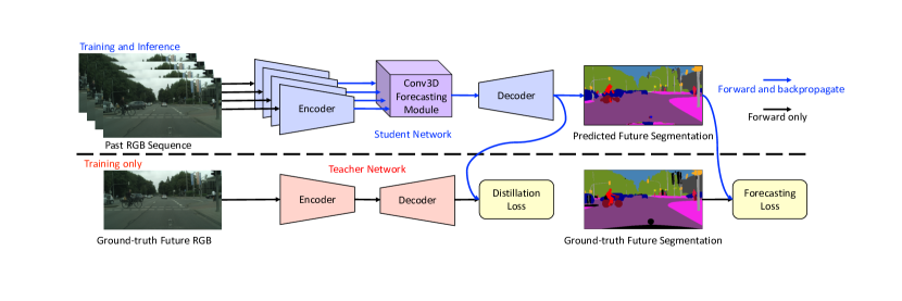
Figure 2: Architecture overview: our student network contains encoder, forecasting module, and decoder to forecast future semantic segmentation. During training, a fixed pre-trained teacher network takes the future RGB frame as input and predicts the future segmentation. The training loss is the weighted sum of the cross-entropy forecasting loss and the mean-squared error distillation loss. During inference, the teacher network is not used and the student network alone performs the forecasting task.

The student network, as shown in the upper half of Fig. 2, has three main components: encoder, forecasting module, and decoder. The encoder generates feature maps in multiple resolutions from each input frame. For a video observed up to time $t$, the inputs are $X_{t-3d}$, $X_{t-2d}$, $X_{t-d}$, and $X_{t}$, where $d$ denotes the displacement between each pair of the preceding frames. The forecasting module uses the feature maps (the lowest level maps from each past frame pathway) to learn a latent-space representation by consolidating temporal dynamics across them. This module uses a temporal 3D convolution structure and acts as a predictive feature learning module integrating feature maps from the preceding frames. Finally, the decoder combines the spatial feature maps (through skip connections to the encoder) and the temporal features (output of the Conv3D module) to generate the final semantic segmentation of the future frame at time $t+d^{\prime}$. Note that $d^{\prime}$ denotes the time delay in the future for which the semantic segmentation is sought. The ground-truth future segmentation is referred to by ${S}_{t+d^{\prime}}$ and the prediction by $\hat{S}_{t+d^{\prime}}$. The choice of $d^{\prime}$ defines how far in the future we plan to segment. We experiment on three different settings of the combinations of $d$ and $d^{\prime}$ for short-term, mid-term, and long-term semantic segmentation forecasting.

The lower half of Fig. 2 shows how the teacher network generates the additional loss term to help train the student network. Unlike X2X [23] that used the future RGB frame as an intermediate training target, our model uses the future frame in a new knowledge distillation approach during training. The teacher network can be any fixed pre-trained single frame semantic segmentation network. It uses the future frame $X_{t+d^{\prime}}$ as the input to predict the future semantic segmentation. The difference between the pre-softmax output features from the teacher network and the one from the student network is used as the additional training loss. During inference, the student network alone is used to define the future segmentation as the output of our model.

3.1 Student Network

This network contains three main components: past encoder, forecasting module, and future decoder to perform our main forecasting task. See the upper half of Fig. 2 and the supplementary material for more details.

Encoder: In contrast to the previous semantic segmentation methods, which are based on encoder-decoder FCN models, our encoder module contains parallel pathways, one for each input preceding frame. Each pathway contains a series of fully convolutional networks, non-linearity layers, and max-pooling layers, to generate multi-resolution feature maps. The encoder can be designed using the common image classification models, such as VGG [32] or ResNet [11], where the feature maps in different resolutions can be extracted right before each max-pooling layer. In our proposed method, we choose VGG19 with batch normalization as our encoder backbone. Please refer to the supplementary material for the architecture details.

Forecasting Module: We introduce a forecasting module to learn predictive features and representations of temporal dynamics. For this purpose, we choose a 3D convolution network Conv3D to combine the encoded feature maps in the lowest resolution of each encoder pathway. This is a simple design choice, but proves to be more accurate than LSTM [8] or ConvLSTM [35] in our experiments. The intuition behind using a Conv3D forecasting module is that it is able to learn more various motion dynamic information. On the contrary, the LSTM-based models always encode all the past information into a fixed size embedding at every timestep. The Conv3D module can access features from any past timesteps and learn to combine them in various ways to model the scene dynamics. This motivates our design of using Conv3D as the forecasting module. In addition to the 3D convolution pathway, skip connections provide another set of interactions between the encoder and the decoder.

Decoder: The decoder takes the encoded feature maps at each resolution and the temporal dynamics representation as inputs and generates the future semantic segmentation, $\hat{S}_{t+d^{\prime}}$. Different decoder structures are used in previous semantic segmentation models. As an example, ConvLSTM [28], reused the decoder of FCN [21] with $1\times 1$ convolution, upsampling, and element-wise addition to obtain the segmentation at the original resolution.

We build our decoder symmetric to the encoder module sequence, as illustrated in the supplementary material. This choice gives us more computation capacity than the FCN decoder. Furthermore, the feature maps from different resolutions of the encoder can be directly concatenated with their counterparts in the decoder pathway maintaining fine boundary information [31, 29]. As a result of this symmetric structure, the lower level feature representation can be fed to the transpose convolution layer, which contains trainable parameters and upsamples the lower resolution feature to a higher resolution. Then, it is concatenated with the encoder feature maps of the corresponding resolution from the latest past time-step followed by 2D convolution modules.

To construct the future segmentation from the decoder, the final convolution layer of the decoder generates a pre-softmax output tensor $O\in\mathbb{R}^{H\times W\times C}$, where $H$ and $W$ are the height and the width of the frames, and $C$ is the number of semantic categories. A soft-max on $O$ generates the predicted probability distribution tensor $P\in\mathbb{R}^{H\times W\times C}$:

$$P(h,w,c)=\frac{\exp(O(h,w,c))}{\sum_{i=1}^{C}\exp(O(h,w,i))},$$ (1)

where $h$, $w$ are the coordinates of a pixel, and $c$ is the index of each semantic class. For each pixel $x=(h,w)\in\{H\times W\}$ and each semantic class $c$, we define the predicted probability function $p_{c}(x)=P(h,w,c)$, where $x=(h,w)$ represents the index of a pixel in the frame. To generate the final forecasting output, we choose the class with the highest probability as our prediction for that pixel. Hence, the predicted category for pixel $x=(h,w)$ at future time $t+d^{\prime}$ is defined as: $\hat{S}_{t+d^{\prime}}(x)=\operatorname*{argmax}_{c}p_{c}(x),$

3.2 Training Loss and Teacher Network

During the training, our loss $L$ is defined as the combination of the forecasting loss $L_{f}$ and the distillation loss $L_{d}$ using weighted sum $L=L_{f}+\lambda L_{d}$, where $\lambda$ is a hyperparameter. The forecasting loss $L_{f}$ measures the difference between the predicted output of the model $\hat{S}_{t+d^{\prime}}$ and the ground-truth semantic segmentation $S_{t+d^{\prime}}$. We use the cross-entropy function to define this classification loss:

$$L_{f}=-\frac{1}{HW}\sum_{x\in\{H\times W\}}\log\left(p_{g(x)}(x)\right),$$ (2)

where $g(x)\in\{1,\ldots,C\}$ defines the ground-truth label for pixel $x$. The second loss term $L_{d}$ is used to measure the difference between the outputs from the student network and the teacher network. The teacher network (lower half of Fig. 2) is a fixed pre-trained single frame segmentation model. The teacher network has the same encoder and decoder architecture as the student network, but without sharing the trainable parameters. The teacher network takes the future RGB frame $X_{t+d^{\prime}}$ as input and generates its own predicted future semantic segmentation $\hat{S}_{t+d^{\prime}}^{te}$. Instead of directly comparing the predicted semantic segmentation, we define the distillation loss $L_{d}$ using the mean squared error between the pre-softmax output tensors from the student network and the teacher network:

$$L_{d}=\frac{1}{HWC}\sum_{h=1}^{H}\sum_{w=1}^{W}\sum_{c=1}^{C}(O(h,w,c)-O_{te}(h,w,c))^{2},$$ (3)

where $O$ is the pre-softmax output tensor from the student network, and $O_{te}$ is the one from the teacher network. With this distillation loss $L_{d}$, the single frame semantic segmentation teacher network provides additional regression guidance for the student network. During training, we minimize the overall loss $L$. During inference, the predicted output of the student network $\hat{S}_{t+d^{\prime}}$ is the final output of our model.

Table 2: Evaluation of our method in terms of mIOU, pixel-level accuracy (pAcc), and mean category accuracy (mAcc) in comparison with baseline and relevant methods on forecasting future semantic segmentation using past RGB sequence as the inputs. In each column, the best obtained results are typeset in boldface and the second best are underlined.

Model	Short-term			Mid-term			Long-term
	mIOU	pAcc	mAcc	mIOU	pAcc	mAcc	mIOU	pAcc	mAcc
Zero-motion	58.91	91.96	69.68	48.15	87.89	59.67	36.21	81.77	47.07
Two-stage	49.17	90.22	61.68	26.53	74.60	36.19	9.64	44.86	14.49
X2X* [23]	-	-	-	23.00	-	-	-	-	-
ConvLSTM** [28]	45.08	89.28	54.15	36.81	85.79	45.57	27.36	80.44	24.63
Ours	65.08	93.83	74.36	56.98	91.38	67.67	40.81	86.03	50.13
*X2X is not the main focus of [23], and only the mid-term mIOU result is reported in this setting.
**Our implementation of [28], using past RGB sequence as the inputs.

4 Experimental Results

Datasets: We first evaluate our method on the Cityscapes [5] dataset. In the training, validation, and testing sets, the dataset provides $2975$, $500$, and $1525$ annotated frames with 19 semantic classes. In each of the video clips of length 30 (frames are indexed 0 to 29), the dataset provides fine annotations for the $19^{\text{th}}$ frame. In total there are 180,000 frames of resolution of $1024\times 2048$ pixels. Following the same setting of [28, 23], we only use the finely annotated frames and downsample the frames to resolution of $256\times 512$. We train our model using the Adam optimizer with initial learning rate of $0.001$, batch size 8, and $\lambda=100$ (the two loss terms will have similar numerical scale in the beginning of training). We initialize the encoder of the student network with ImageNet [7] pre-trained weights.

Apolloscape dataset [13] is also used as an additional experiment, which has 140,000 frames with pixel-level annotations of 22 semantic classes. We extracted 1950 training and 380 validation sequences and down-sampled each frame to resolution of $320\times 384$.

Settings: Following the forecasting settings in the related previous works [23, 28], we design three experimental settings on different time-ranges: short-term, mid-term, and long-term. For all settings, we always define the $19^{\text{th}}$ frame in the Cityscapes sequences, denoted by $S_{19}$, as the forecasting target frame, since the ground-truth semantic labels for this frame is available. The input RGB frames are selected from different timesteps in the past, denoted by $X_{i}$, depending on the forecasting time-range setting For short-term forecasting, the input RGB frames are $X_{15},X_{16},X_{17},X_{18}$; for mid-term forecasting $X_{7},X_{10},X_{13},X_{16}$; and for long-term forecasting they are $X_{1},X_{4},X_{7},X_{10}$, while the output for all is $\hat{S}_{19}$.

Evaluation Metrics: Following previous work, we use the mean Intersection Over Union (mIOU) as the performance metric for segmentation evaluation. We also report pixel-level accuracy (pAcc) and mean per-class accuracy (mAcc). Specifically, mIoU is the pixel IOU averaged across all classes; pAcc defines the percentage of correctly classified pixels; and mAcc is the average class accuracies.

Baseline Methods: We use the ConvLSTM [28] model as the main comparison baseline, which outperforms the previous state-of-the-art S2S [23]. This model achieves the state-of-the-art performance on a slightly different segmentation forecasting task, i.e., , the inputs are the past segmentation sequences. The architecture of ConvLSTM is based on the bidirectional ConvLSTM temporal module and uses the asymmetric Resnet101-FCN encoder-decoder backbone.

Additionally, [23] has an X2X architecture, which is also used as our baseline. It primarily focused on the same problem setting as the one of ConvLSTM [28]. But, they also presented an X2X [23] architecture that uses the past RGB sequences to forecast the future RGB frame and then generate the future segmentation. We argue that it is not necessary to generate the future RGB frame as an intermediate step. Since [23] only presents the result in the mid-term time-range setting, we implement a two-stage model based on the same idea. Another important baseline is denoted by ‘zero-motion.’ This is the case that no motion is anticipated in the video and the future frame semantic segmentation is identical to that of the last observed frame. Although this is a very naïve baseline, it poses as a very challenging one [25, 4], especially for short-term forecasting. To calculate this metric, we first train a single frame semantic segmentation model. Then, we apply it to the last input frame and use the segmentation map as the predicted result.

4.1 Quantitative Results

Table 2 shows the results of our method on the Cityscapes [5] dataset, compared with the previous state-of-the-art. Note that ConvLSTM [28] focused on predicting future segmentation directly from past semantic segmentation as the inputs. Therefore, we re-implemented their model, but training and testing using past RGB sequences as the inputs. As can be seen in Table 2, our model outperforms ConvLSTM by a large margin in all the three time-ranges. That supports our design choice of using the symmetric encoder-decoder backbone and the Conv3D temporal module. We can also see the significant performance difference between the two-stage models, including X2X [23], and our proposed single-stage model. The performance difference supports our argument that forecasting future RGB frame is not necessary for forecasting future semantic segmentation. Besides, our method outperforms the the zero-motion baseline for all three time-ranges. Interestingly, the baselines perform worse than the zero-motion baseline.

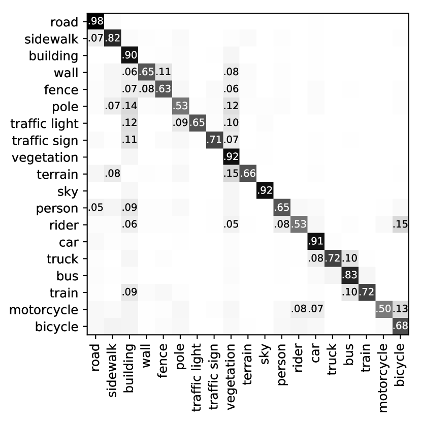
Figure 6: Confusion matrix of the mid-term semantic segmentation forecasting for all 19 classes in the Cityscapes dataset. The x-axis refers to the predicted class labels and the y-axis represents the ground-truth class labels. For instance, the confusion matrix shows that for some cases, the label ‘motorcycle’ is misclassified as ‘bicycle’, ‘rider’, and ‘car’.

In addition to quantitative comparisons with previous works, we analyze our forecasting results for each of the 19 classes of objects. Fig. 3 shows the IOU comparison for all classes over three different forecasting time-ranges, sorted in descending orders. One can notice that the prediction accuracy varies a lot across different classes. To better understand the reasons why certain classes have lower IOUs, we calculate the confusion matrix for all these classes, as shown in Fig. 6 (in the supplementary material). The x-axis in this figure refers to the predicted class labels and the y-axis represents the ground-truth class labels. For instance, the ‘motorcycle’ class, which had the lowest results in Fig. 3 is mainly confused with the ‘bicycle’, ‘rider’, and ‘car’ classes. Additionally, we can see two light gray vertical lines for the ‘building’ and ‘vegetation’ predicted class labels. This shows that other classes are often mistaken with ‘building’ and ‘vegetation’.

Table 3: Ablation results: evaluation of our method in terms of mIOU, pixel-level accuracy (pAcc), and mean category accuracy (mAcc) in comparison with variations of our method on forecasting future semantic segmentation using past RGB sequence as the inputs. In each column, the best obtained results are typeset in boldface and the second best are underlined.

Model	Short-term			Mid-term			Long-term
	mIOU	pAcc	mAcc	mIOU	pAcc	mAcc	mIOU	pAcc	mAcc
Ours w/o symmetric backbone	47.80	89.65	57.31	39.37	87.03	47.72	28.22	81.51	35.95
Ours w/ LSTM	48.22	90.26	58.39	39.57	86.93	49.18	26.61	81.46	33.19
Ours w/ ConvLSTM	58.62	92.92	68.85	47.96	89.29	58.24	34.44	84.21	43.09
Ours w/ Multi-Res Conv3D	59.24	93.24	69.44	49.33	90.38	59.39	36.96	85.42	45.98
Ours w/o distillation loss	63.60	93.76	73.01	55.97	91.17	66.59	40.32	85.84	49.69
Ours w/ 2 input frames	63.85	93.67	73.30	55.67	91.15	66.58	40.37	85.75	50.02
Ours w/ 3 input frames	64.10	93.72	74.18	56.52	91.27	67.26	40.77	85.91	50.11
Ours	65.08	93.83	74.36	56.98	91.38	67.67	40.81	86.03	50.13

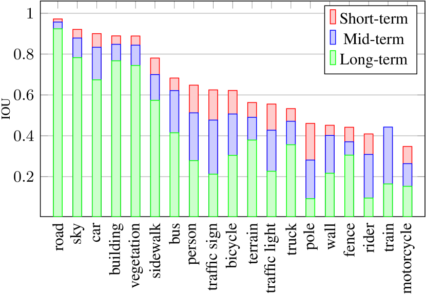
Figure 3: Per-class IOU for all 19 classes with respect to short, mid, and long-term forecasting. The forecasting performance varies a lot across different classes, implying that some classes are more difficult to correctly classify.

Ablation: Table 3 shows the ablation analysis results to examine where the performance improvements derive from. The main differences between our model and previous work are the symmetric encoder-decoder backbone, the Conv3D temporal forecasting module, and the distillation training.

First, to evaluate the symmetric encoder-decoder backbone design, we create another model by replacing our backbone architecture with the asymmetric one as in ConvLSTM [28], which simply uses the decoder of FCN as the decoder (first row of table 3). We can see that all the evaluation metrics are significantly worse than our proposed model. Our proposed symmetric backbone decoder is designed with more computational capacity compared to FCN decoder. The inputs and outputs represent two different types of information (image and segmentation). They are potentially far away from each other in the latent representation space. Therefore, more computation capacity is required, compared with previous works [23, 28] whose inputs and outputs are all segmentation data.

Next we analyze the impact of the temporal structures. We implement three other models by replacing our Conv3D temporal module with LSTM [8], ConvLSTM [35] and the multi-resolution Conv3D. The results are reported in the second, third, and the fourth rows of Table 3. As suggested by the results, the LSTM module has significantly negative impact. ConvLSTM performs much better than LSTM, but still worse than our proposed Conv3D-based temporal module. The multi-resolution Conv3D temporal module contains total five Conv3D layers, each of which takes the past feature maps from different resolution and generates the dynamic information for the decoder. Empirically, we observe that its performance decreases. One possible reason is that the larger number of trainable parameters makes the model prone to over-fitting. Furthermore, this approach requires more memory, which forces the model to operate on a smaller batch size. Therefore, the regularization effect of batch normalization becomes less effective.

Finally, we analyze the impact of the student-teacher architecture and the distillation training loss. Without the teacher network and the distillation training loss, results of our student-only model are shown in the fifth row of Table 3. Our student-only model already outperforms other previous works shown in Table 2. Using the distillation loss of Eq. (3), the mIOU scores further improve by 0.5% to 1.5% mIOU scores for all the three time-range settings

Furthermore, we also experiment on using fewer numbers of input frames, and the results are shown in the sixth and seventh rows in Table 3. Using fewer numbers of input frames decreases the mIOU scores by 0.04% to 1.31%.

Forecasting Segmentation from Past Segmentation: In addition to our main experiments, we also experiment on another simpler task that forecasts future segmentation from past segmentation. This task is the exact problem setting that ConvLSTM [28] achieves the state-of-the-art performance. Our model still outperforms ConvLSTM[28] and another strong baseline, S2S[23], as in Table 4.

Table 4: Comparison of mIOU with S2S [23] and ConvLSTM [28] on forecasting segmentation using past segmentation as input.

Model	Short-term	Mid-term	Long-term
S2S	62.60	59.40	47.80
ConvLSTM	71.37	60.06	-
Ours	72.43	65.53	50.52

Quantitative Results on Apolloscape Dataset: The previous works [23, 28] only experimented on Cityscapes[5]. Additionally, we further experiment on Apolloscape[13], a As shown in Table 5, our proposed model still outperforms ConvLSTM [28]. The distillation training further increases the forecasting performance. Notice that Apolloscape is more challenging compared with Cityscapes as discussed in [13], therefore we see smaller performance gains.

Table 5: mIOU results on Apolloscape dataset.

Model	Short-term	Mid-term	Long-term
Zero-motion	29.87	25.44	19.56
ConvLSTM**	28.27	23.29	17.30
Ours w/o distillation loss	32.26	25.72	20.26
Ours	32.58	26.09	20.47
**Our implementation of ConvLSTM with RGB inputs.

4.2 Qualitative Results

Mid-term Forecasting: We start this section with the mid-term forecasting results, as this is the most widely used setting in the previous work for evaluation. Fig. 4(b) shows the qualitative results, which uses the past RGB sequence $X_{7},X_{10},X_{13},X_{16}$ to forecast the future semantic segmentation at time-step 19, denoted as $S_{19}$. In this figure, each row is a separate sample sequence, and the left most column is the past RGB input sequence, followed by the ground-truth future segmentation, our predicted future semantic segmentation and two other baselines.

$X_{t-3},X_{t-2},X_{t-1},X_{t}$	${S}_{t+1}$: Ground-truth	Ours	ConvLSTM	Two-stage

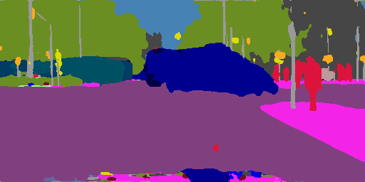
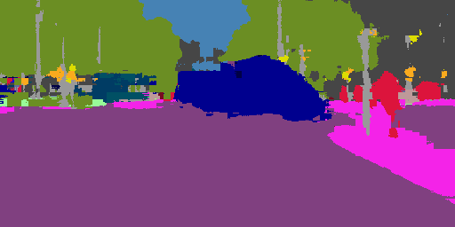
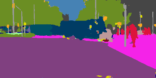
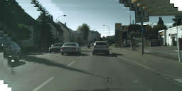
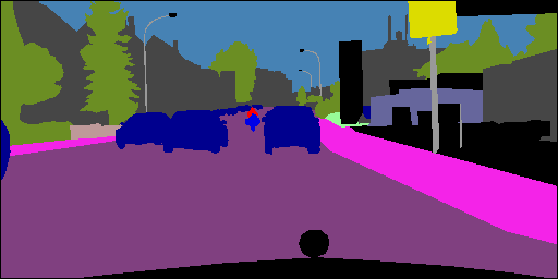
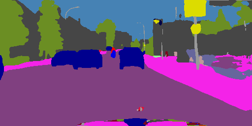
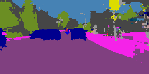
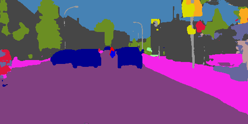
(a) Short-term forecasting results

$X_{t-9},X_{t-6},X_{t-3},X_{t}$	${S}_{t+3}$ Ground-truth	Ours	ConvLSTM	Two-stage

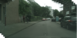
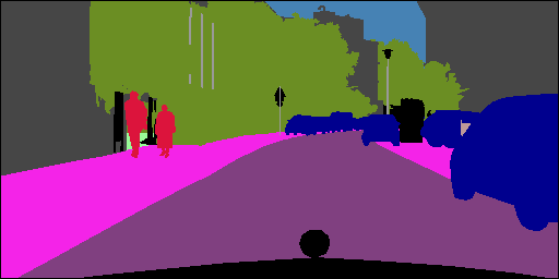
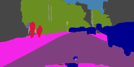
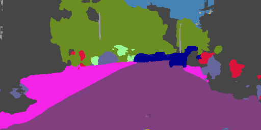
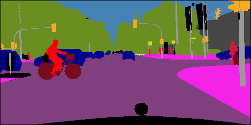
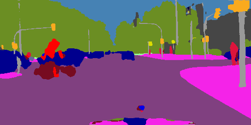
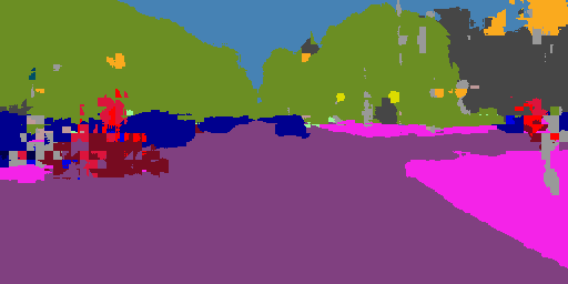
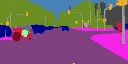
(b) Mid-term forecasting results

$X_{t-9},X_{t-6},X_{t-3},X_{t}$	${S}_{t+9}$ Ground-truth	Ours	ConvLSTM	Two-stage

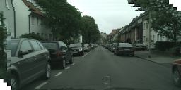
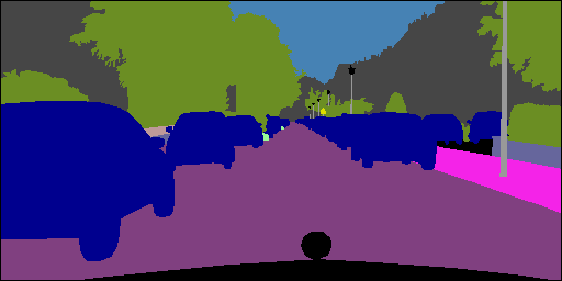
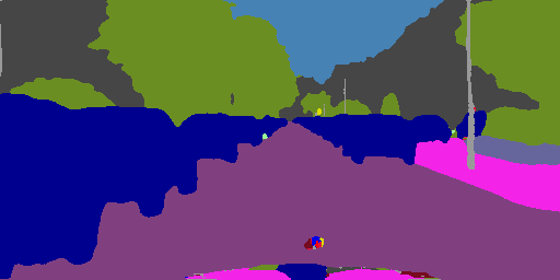
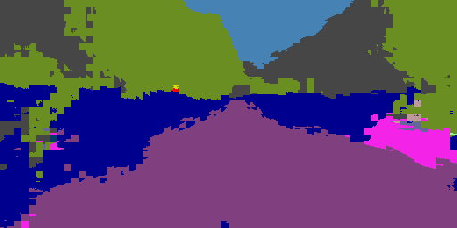
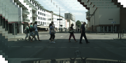
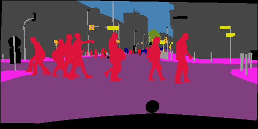
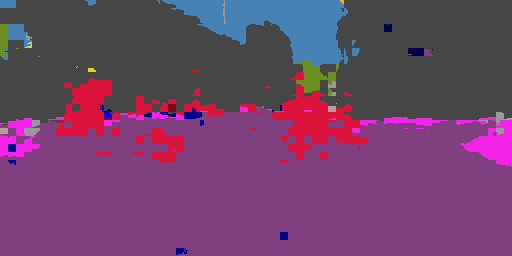
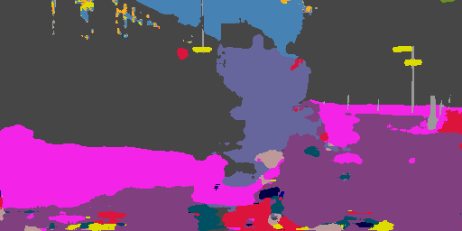
(c) Long-term forecasting results

Figure 4: Qualitative results. $\hat{S}$ denotes the predicted segmentation and $S$ the ground-truth. See supplementary material for more results.

$X$	$\hat{S}_{t+1}$	$\hat{S}_{t+3}$	$\hat{S}_{t+9}$

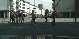
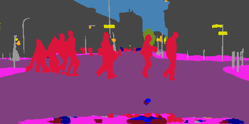
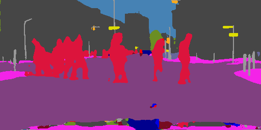
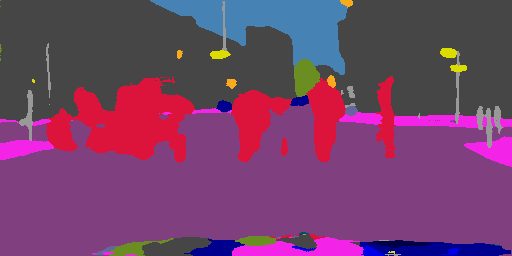
Figure 5: Forecasting results of three different time-range settings for the same sample. $X$ is the last RGB frame; $\hat{S}_{t+1}$, $\hat{S}_{t+3}$, and $\hat{S}_{t+9}$ denote the predicted segmentation of short-, mid-, and long-term settings, corresponding to the same $X$.

The first row shows examples where the camera is moving forward. Our model accurately captures the relative motion dynamic between the camera and all the objects in the scene. Our prediction results show that the right-side street-parking car segmentation moves toward right further, similar to the ground-truth. The second example shows that our model can capture and predict the future based on different motion patterns. In this sample, the camera is relatively static. However, the pedestrians, bike, and cars are moving toward different directions in the scene. Our model is able to distinguish each object and identify their moving directions. Specifically, a biker and a car are moving toward each other. Our model is able to predict these two segments will intersect in the future frame, but was unable to really figure out which one should be in the foreground due to the lack of depth information. This problem can be an interesting future research work, potentially solvable by including additional depth information if provided. More qualitative results can be found in the supplementary material.

Short-term Forecasting: In the short-term setting, we use the past RGB sequence $X_{15},X_{16},X_{17},X_{18}$ to forecast the future semantic segmentation $S_{19}$. Our model precisely predicts both the directions and the magnitude of the movements for the cars, as shown in Fig. 4(a). In the first row, the car is moving toward right, and the predicted car position in the future frame is the same as that in the ground-truth. In the second example, the left parked car is moving out of the frame due to the camera motion. Again, our model captures the exact relative motion dynamic information and precisely forecasts the same shape, size, and location of the area occupied by the same parked car in the future frame. Another interesting issue is that the ground-truth annotation of the second example actually misses the circle direction sign (yellow color in the segmentation map) while our model is capable to detect that direction sign segment and place it in the right position in the future frame.

Long-term Forecasting: In addition, Fig. 4(c) shows the long-term forecasting results. Our model uses the past RGB image sequence $X_{1},X_{4},X_{7},X_{10}$ as the inputs, and generates the future semantic segmentation $S_{19}$, which is 9 steps in the future from the last input frame. Such setting is more challenging than mid-term and short-term forecasting. However, our model can still accurately predict the moving directions of the parked cars (specially in the first example) and the pedestrians in the second example. Although our results correctly predict the moving directions, the magnitude of the movements seem to be smaller than the ground-truth. This may be due to changes in the speeds of the objects in the frames that are not observed by our model.

Time-horizon Comparison: Fig. 5 shows the forecasting results for our three time horizons. For all these settings, we use the same frame, namely $X_{16}$, as the last frame of the input sequence. We forecast the future segmentation at three different time horizon, namely $\hat{S}_{17}$, $\hat{S}_{19}$, and $\hat{S}_{25}$. The short-term forecasting result provides the best visual quality. From the mid-term result, we can still see that the segmentation boundary of the pedestrians are reasonable. But for the long-term result, their shapes start to deform away from regular pedestrian appearance. However, we can still see that different groups of the pedestrians are moving toward their destination in the correct directions, e.g., the left most pedestrian is moving toward left, and the right most pedestrian is moving toward right.

5 Conclusion

In this paper, we proposed a single-stage end-to-end trainable model for the challenging problem of predicting future frame semantic segmentation having only observed the preceding frames RGB data. This is a practical setting for autonomous systems to directly reason about the near future based on current video data without the need to acquire any other forms of meta-data. Our proposed model for solving this task included several encoding pathways to encode the past, a temporal 3D convolution structure for capturing the scene dynamics and predictive feature learning, and finally a decoder to gradually reconstruct the future semantic segmentation. We further proposed a teacher network coupled with a distillation loss for training the network to improve the overall forecasting performance. The results on the popular Cityscapes and Apolloscape datasets indicate that our method can predict future segmentation and outperform several baseline and state-of-the-art methods.

Acknowledgements. This work was partially funded by Panasonic and Oppo. The authors would like to thank Jingwei Ji and Damian Mrowca for their feedback on the paper.

Appendix A Supplementary Material

A.1 More Qualitative Results

Figs. 8,  9,  10 show more qualitative results for short-, mid-, and long-term forecasting, respectively. Each column represents one sample sequence, and the left-most two columns are the same samples from Fig. 4. Here, we also show the all input frames. From the inputs, we can easily observe the movements of different objects, such as pedestrians, cars, and bikes. We can also see that our predicted future semantic segmentation follows the observed motion patterns, and our results are closer to the ground-truth future semantic segmentation for all the three time-range settings. On the contrary, predicted segmentation boundaries by ConvLSTM [28] are not as smooth as ours. The two-stage method only works well for some examples in the short-term forecasting.

A.2 Detailed Network Architecture

Fig. 7 shows the detailed architecture of our proposed network. The encoder module sequence can be seen in Table 6. The forecasting module is a temporal 3D convolution, and the decoder structure is symmetric to the encoder.

Table 6: Summary of one encoder pathway based on VGG19 backbone, applied to an input frame of size $H\times W$. Feature maps are defined as the output of the last convolution module in each block. Column ‘#’ denotes the number of repetitions of that module.

Module Sequence	#	Resolution	Channels
Input Frame		$H\times W$	3
$3\times 3$ Conv2D + BN + ReLU	2	$H\times W$	64
Max-Pool		$\nicefrac{{H}}{{2}}\times\nicefrac{{W}}{{2}}$	64
$3\times 3$ Conv2D + BN + ReLU	2	$\nicefrac{{H}}{{2}}\times\nicefrac{{W}}{{2}}$	128
Max-Pool		$\nicefrac{{H}}{{4}}\times\nicefrac{{W}}{{4}}$	128
$3\times 3$ Conv2D + BN + ReLU	4	$\nicefrac{{H}}{{4}}\times\nicefrac{{W}}{{4}}$	256
Max-Pool		$\nicefrac{{H}}{{8}}\times\nicefrac{{W}}{{8}}$	256
$3\times 3$ Conv2D + BN + ReLU	4	$\nicefrac{{H}}{{8}}\times\nicefrac{{W}}{{8}}$	512
Max-Pool		$\nicefrac{{H}}{{16}}\times\nicefrac{{W}}{{16}}$	512
$3\times 3$ Conv2D + BN + ReLU	4	$\nicefrac{{H}}{{16}}\times\nicefrac{{W}}{{16}}$	512

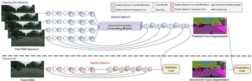
Figure 7: Network architecture overview: our student network contains encoder, forecasting module, and decoder. The encoder takes the past frames and learns latent low-dimensional representations by gradually decreasing the resolution. Our forecasting module then merges them by a temporal 3D convolution that maps them to the future. Finally, the decoder gradually increases the resolution of the output segmentation while having skip connections with the encoder at each resolution. The stacked instances of blue blocks are convolutional modules connected in a sequence. The teacher network has the same encoder and decoder architecture as the student network, but without sharing trainable parameters.

$X_{t-3}$
$X_{t-2}$
$X_{t-1}$
$X_{t}$
${S}_{t+1}$ Ground-truth
Ours
ConvLSTM
Two-stage

Figure 8: More short-term forecasting qualitative results.

$X_{t-9}$
$X_{t-6}$
$X_{t-3}$
$X_{t}$
${S}_{t+3}$ Ground-truth
Ours
ConvLSTM
Two-stage

Figure 9: More mid-term forecasting qualitative results.

$X_{t-9}$
$X_{t-6}$
$X_{t-3}$
$X_{t}$
${S}_{t+9}$ Ground-truth
Ours
ConvLSTM
Two-stage

Figure 10: More long-term forecasting qualitative results.

References

- [1] Alexandre Alahi, Vignesh Ramanathan, and Li Fei-Fei. Socially-aware large-scale crowd forecasting. In CVPR, 2014.
- [2] Apratim Bhattacharyya, Mario Fritz, and Bernt Schiele. Bayesian prediction of future street scenes using synthetic likelihoods. In ICLR, 2019.
- [3] Jingchun Cheng, Yi-Hsuan Tsai, Shengjin Wang, and Ming-Hsuan Yang. Segflow: Joint learning for video object segmentation and optical flow. In ICCV, 2017.
- [4] Hsu-kuang Chiu, Ehsan Adeli, Borui Wang, De-An Huang, and Juan Carlos Niebles. Action-agnostic human pose forecasting. In WACV, 2019.
- [5] Marius Cordts, Mohamed Omran, Sebastian Ramos, Timo Rehfeld, Markus Enzweiler, Rodrigo Benenson, Uwe Franke, Stefan Roth, and Bernt Schiele. The cityscapes dataset for semantic urban scene understanding. In CVPR, 2016.
- [6] Jifeng Dai, Yi Li, Kaiming He, and Jian Sun. R-fcn: Object detection via region-based fully convolutional networks. In NeurIPS, 2016.
- [7] J. Deng, W. Dong, R. Socher, L.-J. Li, K. Li, and L. Fei-Fei. ImageNet: A Large-Scale Hierarchical Image Database. In CVPR, 2009.
- [8] Felix A Gers, Jürgen Schmidhuber, and Fred Cummins. Learning to forget: Continual prediction with lstm. 1999.
- [9] Liang-Yan Gui, Yu-Xiong Wang, Deva Ramanan, and José MF Moura. Few-shot human motion prediction via meta-learning. In ECCV, 2018.
- [10] Agrim Gupta, Justin Johnson, Li Fei-Fei, Silvio Savarese, and Alexandre Alahi. Social gan: Socially acceptable trajectories with generative adversarial networks. In CVPR, 2018.
- [11] Kaiming He, Xiangyu Zhang, Shaoqing Ren, and Jian Sun. Deep residual learning for image recognition. In CVPR, 2016.
- [12] Geoffrey Hinton, Oriol Vinyals, and Jeff Dean. Distilling the knowledge in a neural network. In NeurIPS workshop, 2014.
- [13] Xinyu Huang, Xinjing Cheng, Qichuan Geng, Binbin Cao, Dingfu Zhou, Peng Wang, Yuanqing Lin, and Ruigang Yang. The apolloscape dataset for autonomous driving. In CVPR, 2018.
- [14] Xiaojie Jin, Xin Li, Huaxin Xiao, Xiaohui Shen, Zhe Lin, Jimei Yang, Yunpeng Chen, Jian Dong, Luoqi Liu, Zequn Jie, et al. Video scene parsing with predictive feature learning. In ICCV, 2017.
- [15] Xiaojie Jin, Huaxin Xiao, Xiaohui Shen, Jimei Yang, Zhe Lin, Yunpeng Chen, Zequn Jie, Jiashi Feng, and Shuicheng Yan. Predicting scene parsing and motion dynamics in the future. In NeurIPS, 2017.
- [16] Nal Kalchbrenner, Aaron van den Oord, Karen Simonyan, Ivo Danihelka, Oriol Vinyals, Alex Graves, and Koray Kavukcuoglu. Video pixel networks. arXiv preprint arXiv:1610.00527, 2016.
- [17] Kris M Kitani, Brian D Ziebart, James Andrew Bagnell, and Martial Hebert. Activity forecasting. In ECCV, 2012.
- [18] Abhijit Kundu, Vibhav Vineet, and Vladlen Koltun. Feature space optimization for semantic video segmentation. In CVPR, 2016.
- [19] Yi Li, Haozhi Qi, Jifeng Dai, Xiangyang Ji, and Yichen Wei. Fully convolutional instance-aware semantic segmentation. In CVPR, 2017.
- [20] Tsung-Yi Lin, Piotr Dollár, Ross B Girshick, Kaiming He, Bharath Hariharan, and Serge J Belongie. Feature pyramid networks for object detection. In CVPR, 2017.
- [21] Jonathan Long, Evan Shelhamer, and Trevor Darrell. Fully convolutional networks for semantic segmentation. In CVPR, 2015.
- [22] Pauline Luc, Camille Couprie, Yann Lecun, and Jakob Verbeek. Predicting future instance segmentations by forecasting convolutional features. 2018.
- [23] Pauline Luc, Natalia Neverova, Camille Couprie, Jakob Verbeek, and Yann LeCun. Predicting deeper into the future of semantic segmentation. In ICCV, 2017.
- [24] Zelun Luo, Jun-Ting Hsieh, Lu Jiang, Juan Carlos Niebles, and Li Fei-Fei. Graph distillation for action detection with privileged information. In ECCV, 2018.
- [25] Julieta Martinez, Michael J Black, and Javier Romero. On human motion prediction using recurrent neural networks. In CVPR, 2017.
- [26] Michael Mathieu, Camille Couprie, and Yann LeCun. Deep multi-scale video prediction beyond mean square error. In ICLR, 2016.
- [27] Ehsan Adeli Mosabbeb, Maryam Sadeghi, and Mahmoud Fathy. A new approach for vehicle detection in congested traffic scenes based on strong shadow segmentation. In International Symposium on Visual Computing, pages 427–436. Springer, 2007.
- [28] Seyed Shahabeddin Nabavi, Mrigank Rochan, and Yang Wang. Future semantic segmentation with convolutional lstm. In BMVC, 2018.
- [29] Dong Nie, Li Wang, Ehsan Adeli, Cuijin Lao, Weili Lin, and Dinggang Shen. 3-d fully convolutional networks for multimodal isointense infant brain image segmentation. IEEE Transactions on Cybernetics, 2018.
- [30] Shaoqing Ren, Kaiming He, Ross Girshick, and Jian Sun. Faster r-cnn: Towards real-time object detection with region proposal networks. In NeurIPS, 2015.
- [31] Olaf Ronneberger, Philipp Fischer, and Thomas Brox. U-net: Convolutional networks for biomedical image segmentation. In MICCAI, 2015.
- [32] Karen Simonyan and Andrew Zisserman. Very deep convolutional networks for large-scale image recognition. arXiv preprint arXiv:1409.1556, 2014.
- [33] Jonathan C. Stroud, David A. Ross, Chen Sun, Jia Deng, and Rahul Sukthankar. D3d: Distilled 3d networks for video action recognition. arXiv preprint arXiv:1812.08249, 2018.
- [34] Carl Vondrick, Hamed Pirsiavash, and Antonio Torralba. Anticipating visual representations from unlabeled video. In CVPR, 2016.
- [35] SHI Xingjian, Zhourong Chen, Hao Wang, Dit-Yan Yeung, Wai-Kin Wong, and Wang-chun Woo. Convolutional lstm network: A machine learning approach for precipitation nowcasting. In NeurIPS, 2015.
- [36] Sergey Zagoruyko, Adam Lerer, Tsung-Yi Lin, Pedro O Pinheiro, Sam Gross, Soumith Chintala, and Piotr Dollár. A multipath network for object detection. arXiv preprint arXiv:1604.02135, 2016.
- [37] Kuo-Hao Zeng, William B Shen, De-An Huang, Min Sun, and Juan Carlos Niebles. Visual forecasting by imitating dynamics in natural sequences. In ICCV, 2017.
- [38] Chenxi Zhang, Liang Wang, and Ruigang Yang. Semantic segmentation of urban scenes using dense depth maps. In ECCV, 2010.
- [39] Hang Zhang, Kristin Dana, Jianping Shi, Zhongyue Zhang, Xiaogang Wang, Ambrish Tyagi, and Amit Agrawal. Context encoding for semantic segmentation. In CVPR, 2018.
- [40] Peng Zhang, Jiuling Wang, Ali Farhadi, Martial Hebert, and Devi Parikh. Predicting failures of vision systems. In CVPR, 2014.
- [41] Sihang Zhou, Dong Nie, Ehsan Adeli, Yaozong Gao, Li Wang, Jianping Yin, and Dinggang Shen. Fine-grained segmentation using hierarchical dilated neural networks. In MICCAI, 2018.