Electron and positron spectra in the three dimensional spatial-dependent propagation model

Abstract

The spatial-dependent propagation model has been successfully used to explain diverse observational phenomena, including the spectral hardening of cosmic-ray nuclei above $200$ GV, the large-scale dipole anisotropy and the diffusive gamma distribution. In this work, we further apply the spatial-dependent propagation model to both electrons and positrons. To account for the excess of positrons above $10$ GeV, an additional local source is introduced. And we also consider a more realistic spiral distribution of background sources. We find that due to the gradual hardening above $10$ GeV, the hardening of electron spectrum above tens of GeV can be explained in the SDP model and both positron and electron spectra less than TeV energies could be naturally described. The spatial-dependent propagation with spiral-distributed sources could conforms with the total electron spectrum in the whole energy. Meanwhile compared with the conventional model, the spatial-dependent propagation with spiral-distributed sources could produce larger background positron flux, so that the multiplier of background positron flux is $1.42$, which is much smaller than the required value by the conventional model. Thus the shortage of background positron flux could be solved. Furthermore we compute the anisotropy of electron under spatial-dependent propagation model, which is well below the observational limit of Fermi-LAT experiment.

1 Introduction

The conventional cosmic-ray propagation model predicts that the observed energy spectrum falls as a featureless power law, i.e. $\propto R^{-\nu-\delta}$, with $\nu$ and $\delta$ being the power indexes of the injection spectrum and diffusion coefficient respectively. However more and more observations disfavor such simple picture. First of all, a significant excess of positrons above $10$ GeV was discovered by the PAMELA experiment (Adriani et al., 2009). Before long this anomaly was substantiated by the Fermi-LAT experiment (Abdo et al., 2009). The recent observations from the AMS-02 collaboration extended the measurements up to $600$ GeV with an unprecedented high precision (Accardo et al., 2014; Aguilar et al., 2014a). On the other hand, the comprehensive analysis to the AMS-02 electron data (Li et al., 2015) indicate an additional component above $\sim 50$ GeV, which has been observed by the DAMPE satellite (Chang et al., 2008). Moreover, the HESS experiment reported that there is a spectral break around $1$ TeV in the total electron spectrum (electron + positron), which resembled the knee region at $\sim 4$ PeV in the spectrum of cosmic ray nuclei (Aharonian et al., 2009). This sign was also observed by other experiments such as MAGIC, VERITAS and the latest DAMPE (Borla Tridon, 2011; Staszak et al., 2015; Chang et al., 2008).

The overabundance of positrons has called a lot of attention, which implies the existence of extra primary sources. A number of models have been proposed to explain the PAMELA and AMS-02 observations, which can be either astrophysical, such as local pulsars (Shen, 1970; Zhang & Cheng, 2001; Yüksel et al., 2009; Hooper et al., 2009; Yuan et al., 2015; Profumo, 2012; Guo et al., 2015) and the hadronic interactions inside SNRs (Blasi, 2009; Fujita et al., 2009; Hu et al., 2009; Tomassetti & Donato, 2015), or more exotic origins like the dark matter self-annihilation or decay (Bergström et al., 2008; Cirelli et al., 2009; Barger et al., 2009; Yin et al., 2009; Bergström et al., 2009; Zhang et al., 2009). For an extensive introduction of relevant models, one can refer to the reviews (He, 2009; Fan et al., 2010; Serpico, 2012; Cirelli, 2012; Bi et al., 2013) and references therein. Additionally, the $e^{+}/e^{-}$ ratio can also be interpreted as the charge-sign dependent particle injection and acceleration (Malkov et al., 2016). For the drop-off of electron spectrum, it is argued to be caused by the radiation cooling of electrons surrounding SNRs (Vannoni et al., 2009) or the threshold interaction during the transport of cosmic ray electrons (Hu et al., 2009; Wang et al., 2010; Jin et al., 2016).

The spatial-dependent propagation (SDP) model was first used to describe the spectral hardening of primary cosmic-ray proton and helium above $200$ GV which are observed successively by ATIC-2 (Panov et al., 2006, 2009), CREAM (Ahn et al., 2010; Yoon et al., 2011, 2017) and PAMELA (Adriani et al., 2011) and AMS-02 (Aguilar et al., 2015b, a) experiments. This scenario was initially introduced by Tomassetti (2012) as Two Halo model (THM). In this model, the whole transport volume is divided into two regions. The Galactic disk and its surrounding area are called the inner halo (IH), in which the diffusion property is influenced by the CR sources. Outside of IH, the diffusion approaches to the traditional assumption, i.e. only rigidity dependent. This extensive region is named as outer halo (OH). To reproduce the high energy excess, the diffusion coefficient within IH has a weaker rigidity dependence on average, compared with OH zone. In addition to the spectral hardening, the SDP model is further applied to solve the puzzles of large-scale anisotropy, diffuse gamma ray distribution and so forth (Tomassetti, 2012; Guo et al., 2016; Guo & Yuan, 2018; Liu et al., 2018; Qu, 2019).

In this work, we further study the SDP model by applying to the observations of CR electrons and positrons. To account for the excess of positrons above $10$ GeV, a nearby young source is introduced. Meanwhile to better compute the fluxes of background electrons and positrons, we further consider a more realistic spiral distribution of sources. We compare three kinds of transport model: conventional, SDP and SDP plus spiral distribution. We find that under traditional axisymmetric distribution of sources, both conventional and SDP models could not well explain the spectra of both positron and electron with only a local source, and an extra electron component is needed. But with a spiral distribution, the SDP model could well describe the spectra of electrons, positrons as well as the total. We also find that in this case, the required enhancement of background positron flux is only $1.42$, which is much smaller than the conventional model. We further compute the anisotropy of electron and find that SDP model predicts a much smaller amplitude of anisotropy.

The rest paper is organized in the following way. In Sec.2, both spatial-dependent propagation model and spiral distribution of sources are presented in detail. Sec.3 gives the calculated results and Sec.4 is reserved for the conclusion.

2 Model Description

2.1 Spatial-dependent propagation

After escaping into the interstellar space, CRs diffuse within the Galaxy by randomly scattering off magnetic waves and MHD turbulence. Besides diffusion, CRs still experience reacceleration, convection, fragmentation, radioactive decay and energy losses before arriving at earth. The corresponding propagation process could be described by a so-called diffusion equation:

$$\dfrac{\partial\psi(\textbf{r},p,t)}{\partial t} =q(\textbf{r},p,t)+\nabla\cdot(D_{xx}\nabla\psi-V_{c}\psi)$$

$$+\dfrac{\partial}{\partial p}p^{2}D_{pp}\dfrac{\partial}{\partial p}\frac{1}{p^{2}}\psi-\dfrac{\partial}{\partial p}\left[\dot{p}\psi-\dfrac{p}{3}(\nabla\cdot V_{c}\psi)\right]$$

$$-\dfrac{\psi}{\tau_{f}}-\dfrac{\psi}{\tau_{r}}~{}.$$ (1)

with $\psi(\textbf{r},p,t)$ the CR density per unit momentum $p$ at position r. $\tau_{f}$ and $\tau_{r}$ are the characteristic timescales for fragmentation and radioactive decay respectively. $V_{c}$ is the convention velocity. In the diffusive-reacceleration term, $D_{pp}$ is related to $D_{xx}$ by the formula $D_{pp}D_{xx}=\dfrac{4p^{2}v_{A}^{2}}{3\delta(4-\delta^{2})(4-\delta)}$, in which $v_{A}$ is the Alfvén velocity (Seo & Ptuskin, 1994). In this work, we adopt the common diffusion-reacceleration model, which is called DR for short. The diffusive halo is approximated as a flat cylinder with the radius of $R=20$ kpc. The half-thickness $z_{h}$ of halo is determined by fitting the B/C ratio.

The CR sources are distributed in the middle of diffusive halo. $q(\textbf{r},p,t)$ represents the source term of CR particles. The spatial distribution of CR sources is paramterized as

$$f(r,z)=\left(\dfrac{r}{r_{\odot}}\right)^{\alpha}\exp\left[-\dfrac{\beta(r-r_{\odot})}{r_{\odot}}\right]\exp\left(-\dfrac{|z|}{z_{s}}\right)~{},$$ (2)

with $r_{\odot}=8.5$ kpc, $\alpha=1.09$, and $\beta=3.87$ (Green, 2015) respectively. In the direction perpendicular to the Milky Way, the number of SNRs decays as an exponential function, with a mean value $z_{s}=100$ pc. To fit the low energy spectra, the injection spectra of proton and electron are assumed to have a broken power-law respectively:

$$q^{\rm p}({\cal R})=q^{\rm p}_{0}\left\{\begin{array}[]{lll}&\left(\dfrac{{\cal R}}{{\cal R}_{\rm br}^{\rm p}}\right)^{\nu_{1}^{\rm p}},&{{\cal R}\leq{\cal R}_{\rm br}^{p}}\\ \\ &\left(\dfrac{{\cal R}}{{\cal R}_{\rm br}^{\rm p}}\right)^{\nu_{2}^{\rm p}}\exp\left[-\dfrac{{\cal R}}{{\cal R}_{\rm c}^{\rm p}}\right],&{{\cal R}>{\cal R}_{\rm br}^{\rm p}}\end{array}\right.$$ (3)

and

$$q^{\rm e}({\cal R})=q^{\rm e}_{0}\left\{\begin{array}[]{lll}\left(\dfrac{{\cal R}}{{\cal R}_{\rm br}^{\rm e}}\right)^{\nu_{1}^{\rm e}},&{{\cal R}\leq{\cal R}_{\rm br}^{\rm e}}\\ \\ \left(\dfrac{{\cal R}}{{\cal R}_{\rm br}^{\rm e}}\right)^{\nu_{2}^{\rm e}}\exp\left[-\dfrac{R}{R_{\rm c}^{\rm e}}\right],&{{\cal R}>{\cal R}_{\rm br}^{\rm e}}\\ \end{array}\right.$$ (4)

where $\nu$ and $q_{0}$ are the spectral index and normalization for proton(electron) respectively, and $R_{\rm c}$ is the cut-off rigidity.

In the SDP model, the half-thickness of inner and outer halo are $\xi z_{h}$ and $(1-\xi)z_{h}$ respectively (Tomassetti, 2012). Within the inner halo, the magnitude of diffusion is supposed to have an anti-correlation with the radial distribution of background CR sources. The corresponding diffusion coefficient $D_{xx}$ is thus parameterized as:

$$D_{xx}(r,z,\mathcal{R})=D_{0}F(r,z)\beta^{\eta}\left(\dfrac{\mathcal{R}}{\mathcal{R}_{0}}\right)^{\delta(r,z)}~{}.$$ (5)

Both $F(r,z)$ and $\delta(r,z)$ are anti-correlated with the source density (Guo & Yuan, 2018), which are paramterized as

$$F(r,z)=\begin{cases}g(r,z)+\left[1-g(r,z)\right]\left(\dfrac{z}{\xi z_{0}}\right)^{n},&|z|\leqslant\xi z_{0}\\ 1,&|z|>\xi z_{0}\end{cases},\\$$ (6)

$$\delta(r,z)=\begin{cases}g(r,z)+\left[\delta_{0}-g(r,z)\right]\left(\dfrac{z}{\xi z_{0}}\right)^{n},&|z|\leqslant\xi z_{0}\\ \delta_{0},&|z|>\xi z_{0}\end{cases},$$ (7)

in which $g(r,z)=N_{m}/[1+f(r,z)]$. Outside the IH region, the turbulence is believed to be CR-driven in principle. Hence the diffusion is regarded as only rigidity dependent, namely $D_{xx}=D_{0}\beta^{\eta}(\mathcal{R}/\mathcal{R}_{0})^{\delta_{0}}$.

2.2 Spiral distribution of CR sources

In the usual transport model, the CR sources are regarded as axisymmetric-distributed. This assumption is rational when the diffusion length of CRs is much larger than the characteristic distance between the adjacent spiral arms. However subject to the severe energy loss, the transport distance of the energetic electrons is much shorter. In this case, the specific position of the solar system and its neighbouring source distribution are expected to notably affect the observed spectrum of cosmic-ray electrons. Now it is widely accepted that our Galaxy is a typical spiral galaxy, in which the high-density gas inside spiral arms trigger the rapid star formation. So the cosmic-ray sources are highly concentrated in the spiral arms. There are still some uncertainties in the structure of the spiral arms, owing to our position in the Galaxy. While the outer part of the Milky Way seems to have four arms, the number of arms in the inner part is still being debated. The measurements for the spiral structure and number of spiral arms are reviewed in (Vallee, 1995; Elmegreen, 1998; Vallée, 2002, 2017). The influences of spiral-distributed sources have been investigated in the recent studies (Shaviv, 2002; Shaviv et al., 2009; Blasi & Amato, 2012; Effenberger et al., 2012; Gaggero et al., 2013; Benyamin et al., 2014; Kopp et al., 2014; Werner et al., 2015; Liu et al., 2015; Kissmann et al., 2015; Benyamin et al., 2016; Porter et al., 2017; Nava et al., 2017).

In this work, we adopt the spiral model established by (Faucher-Giguère & Kaspi, 2006). The whole Galaxy is considered to be made of four major arms spiraling outward from the Galactic center, as shown in Fig. 1. For the $i$-th arm centroid, the locus can be expressed analytically by the logarithmic curve: $\theta(r)=k^{i}\ln(r/r^{i}_{0})+\theta_{0}^{i}$, where $r$ is the distance to the Galactic center. Table 1 lists the values of $k^{i}$, $r^{i}_{0}$ and $\theta_{0}^{i}$ for the each arm. Along the spiral arm, there is a spread in the radial coordinate that follows a normal distribution

$$f_{i}=\dfrac{1}{\sqrt{2\pi}\sigma}\exp\left(-\dfrac{(r-r_{i})^{2}}{2\sigma^{2}}\right)~{},~{}~{}~{}i\in[1,2,3,4]~{},$$ (8)

where $r_{i}$ is the inverse function of the locus of the $i$-th spiral arm and the standard deviation $\sigma$ is taken to be $0.07r_{i}$. The density of CR sources at different radii is proposed to conform with the radial distribution under axisymmetric case. The solar system lies between the Carina-Sagittarius spiral centroid and Perseus spiral centroid.

Fig. 1: Spiral distribution of CR sources in the Milky Way. The Galaxy is assumed to have four spiral arms, with the Sun lying between the Carina-Sagittarius and Perseus arms, about $8.5$ kpc away from the Galactic center.

Tab. 1: The values of the parameters $k^{i}$, $r^{i}_{0}$ and $\theta_{0}$ for four Galactic arm centroids

$i$-arm	name	$k^{i}$ (rad)	$r^{i}_{0}$ (kpc)	$\theta_{0}^{i}$ (rad)
1	Norma	4.25	3.48	0
2	Carina-Sagittarius	4.25	3.48	4.71
3	Perseus	4.89	4.90	4.09
4	Crux-Scutum	4.89	4.90	0.95

2.3 Local source

To account for the excess of positron above $10$ GeV, we consider a pulsar nearby the solar system, which injects the electron and positron pairs instantaneously. The injection spectrum of this pulsar is assumed to be a power law:

$$Q(E)=Q_{0}\left(\dfrac{E}{1~{}\rm GeV}\right)^{-\gamma}~{}.$$ (9)

3 Results

3.1 B/C ratio and proton spectrum

First of all, to determine the transport parameters, the ratio of B/C is fitted, which are illustrated in the Fig. 2. The orange, blue and black solid lines correspond to the models of the conventional, SDP and SDP plus spiral-distributed sources respectively. The fitted transport parameters are listed in table 2. Compared with the conventional picture, the SDP scenarios expect that the B/C ratio could arise above TeV energies, which are clearly visible in the figure.

Fig. 3 shows the corresponding proton spectra. The red squares and gray inverted triangles are from the AMS-02 (Aguilar et al., 2015b) and CREAM experiments (Yoon et al., 2017). The conventional model predicts a single power-law above tens of GeV. In contrast, under SDP model, the propagation of energetic CRs is dominated by IH region, in which the rigidity dependence of the diffusion coefficient is flatter than outside. Thus in this case the proton spectra show a significant hardening above $\sim 200$ GeV, which could well reproduce the observations of both AMS-02 and CREAM experiments. Moreover, we could see that the distribution of sources make no difference to the proton flux at lower energies. Since the diffusion length of low energy protons is much longer than the distance between two neighbouring spiral arms, the distribution of CR sources does not prominently affect the spectrum. But for high energy protons, the major diffusion region is at the IH region, whose thickness is comparable to the distance between two neighbouring spiral arms, the source distribution could not be neglected. It can be seen that at TeV energies, the spiral distribution could produce a harder spectrum. The parameters of proton injection spectrum are listed in table 2.

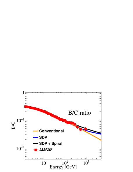
Fig. 2: The fitting to the B/C ratio under three propagation models, which are conventional(orange), SDP(blue) and SDP plus spiral-distributed sources(black) respectively. The data of AMS-02 experiment are taken from (Aguilar et al., 2015b).

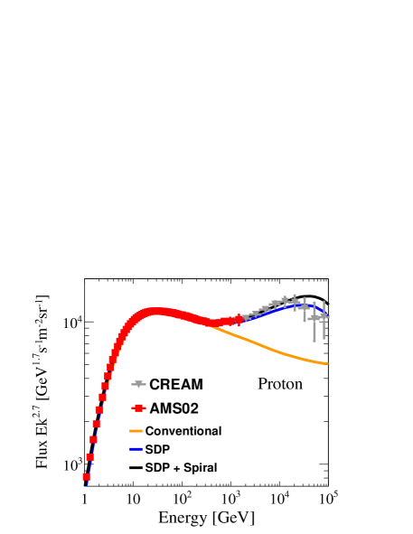
Fig. 3: The proton spectra under three propagation models, i.e. conventional(orange), SDP(blue) and SDP plus spiral-distributed sources(black). The experiment data are taken from AMS-02 (red square) (Aguilar et al., 2015b, 2017) and CREAM (grey inverted triangle) (Ahn et al., 2009; Yoon et al., 2017).

Tab. 2: The parameters for three different models including propagation and injection spectrum of proton

Parameters	SDP+spiral	SDP+axisymmetric	conventional
$D_{0}$	9.87	4.6	5.82
$\delta_{0}$	0.65	0.6	0.6
$z_{h}$[kpc]	6	5	4
$N_{m}$	0.27	0.17
$v_{A}$ [km$\cdot$$s^{-1}$]	6	6	30
$q_{0}^{\rm p}[\rm cm^{-2}sr^{-1}s^{-1}GeV^{-1}]$	4.32$\times 10^{-2}$	4.36$\times 10^{-2}$	4.45$\times 10^{-2}$
$\nu_{1}^{\rm p}$	2.0	2.0	1.75
$\nu^{\rm p}_{2}$	2.3	2.4	2.25
${\cal R}_{\rm br}^{\rm p}$ [GV]	5.5	5.5	9.9
$\phi^{\rm p}$[MV]	830	830	560

3.2 Spectra of electron and positron

In Fig. 4, we compare the positron spectra under three transport models. The red squares are from AMS-02 experiment (Aguilar et al., 2014a). The blue and green solid lines are the contributions from background and local sources resepctively. Since the background positron flux is much lower, the observed positron data could not be described even with a local source. This could be caused by the possible uncertainties from the hadronic interactions, propagation models, the ISM density distributions, and the nuclear enhancement factor from heavy elements. In this work, the background positron flux is multiplied by a factor $c^{e^{+}}$, which is shown as a blue dash-dot lines. The black line is the sum of enhanced background and local fluxes. We could find that under the SDP model, the yield of second positrons is appreciably more than the conventional model. Therefore, the required enhancement factor $c^{e^{+}}$ in SDP model is only $1.92$ and $1.42$, smaller than the traditional model. Compared with axisymmetric case, $c^{e^{+}}$ under the spiral distribution is smaller. Meanwhile like proton, the propagated secondary positrons becomes hardening above tens of GeV. But due to the energy loss of positron during the transport, the broken energy shifts from $200$ GeV to $20$ GeV. Table 3 lists the distance and age of local source as well as the parameters for the corresponding injection spectrum.

Fig. 4: The positron spectra computed under under three transport models, i.e. conventional (upper left), SDP (upper right), SDP + spiral distribution (lower left). The red squares are the measurements from the AMS-02 experiment (Aguilar et al., 2014a). The blue and green solid lines represents the fluxes from the background and the local sources respectively. To well describe the positron flux, the background fluxes are multiplied by a factor $c^{e^{+}}$, which are shown as the dash-dot blue lines.

Fig.5 shows the corresponding electron spectra under three transport models. The red squares are the AMS-02 experiment (Aguilar et al., 2014a). The blue and green solid lines are the contributions from background and local sources resepctively, while the black line is the sum of them. It can be seen that under conventional model, the computed electron flux could not explain the observational data, even with only a local source. It can be inferred that an additional electron component is needed in the case of the conventional transport scenario (Liu et al., 2017). This is also indicated by the analysis of Li et al. (2015). But under the SDP model, the calculated electron flux conforms with the observation much better. This is because that the propagated electron spectra has a hardening above $\sim 10$ GeV, which elevates the background electron flux. With spiral-distributed sources, the electron flux could well describe the observed electron flux. The parameters of injection spectrum of primary electrons from background and local sources for three propagation models are also given in Table 3.

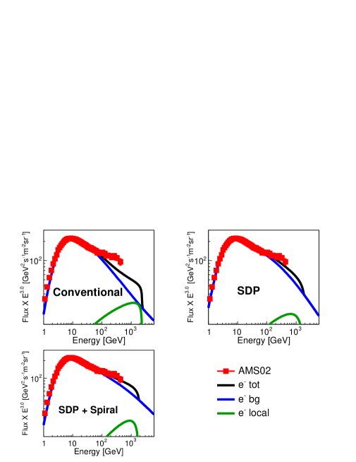
Fig. 5: The electron spectra computed under under three transport models, i.e. conventional (upper left), SDP (upper right), SDP + spiral distribution (lower left). The red squares are the measurements from the AMS-02 experiment (Aguilar et al., 2014a). The blue and green solid lines represents the fluxes from the background and the local sources respectively.

Fig. 6 further shows the total electron spectra computed by different propagation models in comparison with AMS-02 (Aguilar et al., 2014b) and HESS experiments. The orange, blue and black solid lines correspond to the conventional, SDP and SDP with spiral distribution respectively. In the conventional model, the obtained background electron flux is a single power-law, which is not enough for the high-energy electron component. For the SDP model, the traditional distribution of sources could marginally explain both electron and positron spectra less then TeV energies. But when considering the latest observations of HESS, it is still not enough. By introducing a spiral distribution, the high energy electron flux has been significantly boosted. We could see that the SDP plus spiral distribution can well reproduce total electron spectrum within the whole energy range, compared with the other two models. It is noteworthy that there is a sharp break around several TeV for each model, which are brought about by the plummet of local flux. This is caused by our simplified cooling time of electron, which is fixed to $10^{16}$s. When considering the distribution of background photons, the sharp break is expected to disappear.

Fig. 6: The total electron spectra (electron + positron) computed by three transport models, i.e. conventional (orange), SDP (blue), SDP + spiral distribution (black). The red squares and green inverted triangle are the measurements from the AMS-02 (Aguilar et al., 2014b) and HESS experiments respectively.

Tab. 3: The parameters of injection spectrum for background electron and local electron and positron

parameters	SDP+spiral	SDP+axisymmetric	conventional
$q_{0}^{\rm e^{-}}[\rm cm^{-2}sr^{-1}s^{-1}GeV^{-1}]$	0.30	0.30	0.16
$\nu_{1}^{\rm e^{-}}$	1.14	1.53	1.69
$\nu^{e^{-}}_{2}$	2.72	2.89	2.81
${\cal R}_{\rm br}^{\rm e^{-}}$ [GV]	4.6	4.6	4
$r$ [kpc]	0.25	0.21	0.21
$t$ [yr]	1.7$\times 10^{5}$	1.7$\times 10^{5}$	1.3$\times 10^{5}$
$Q_{0}$ [GeV-1]	1.9$\times 10^{50}$	2.7$\times 10^{50}$	2.7$\times 10^{50}$
$\gamma$	2.46	2.60	1.84
$c^{e^{+}}$	1.42	1.92	3.5
$\phi^{\rm e^{+}}$[MV]	650	690	1300
$\phi^{\rm e^{-}}$ [MV]	650	650	1250

3.3 Anisotropy of electron

We further calculate the dipole anisotropies of electron as a function of energy under these propagation models. The dipole anisotropy is usually defined as

$$\delta=\frac{3D_{xx}}{v}\dfrac{|\nabla\psi|}{\psi}~{}.$$ (10)

Due to the distribution of Galactic SNRs with a higher density at the inner Galactic disk, there is inevitably a radial gradient of CR density from the direction of the Galactic center. Thereupon in the scenario of steady-state propagation, the anisotropy scales with the diffusion coefficient so that it grows with the energy.

Fig.7 illustrates the anisotropies of electron when the local source is in the direction of Galactic center. The orange, blue and black solid lines show the anisotropies under the conventional, SDP and SDP+spiral distribution respectively. In the conventional model, due to a larger diffusion coefficient, the expected background anisotropy is obviously large. When the local source is at the direction of Galactic center, its influence to the total anisotropy is inconspicuous, while the background has an overwhelming contribution, as shown in the left figure. In this case, the total anisotropy is close to the observed upper limit by the Fermi-LAT experiment.

Different from the conventional model, the background anisotropy under SDP model is well below the current upper limit. This is due to the slower diffusion coefficient around the Galactic disk. Compared with the axisymmetric case, the spiral distribution induces a larger background anisotropy. From the figure, it can be seen that the anisotropy from the local source is much larger between $100$ and $1000$ GeV. Even so, the total anisotropy is still much smaller. The current and future experiments, which observe the electrons, for example DAMPE and LHAASO, could test our model.

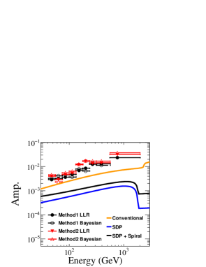
Fig. 7: Anisotropies of electron with the local source at the direction of Galactic center. The orange, blue and black solid lines show the anisotropies under the conventional, SDP and SDP+spiral distribution respectively. The upper limits are from the Fermi-LAT experiment (Abdollahi et al., 2017), which are shown as the black and red markers.

4 Conclusion

With the development of instruments, the detections of cosmic-ray electron and positron have been greatly improved in these recent years. The precise measurements unveil some interesting features and raise the new challenges for the traditional propagation model.

In this work, we apply the SDP + local source model to study both electron and positron spectra. We also introduce the spiral model to account for more realistic distribution of CR sources. We find that even with one local source, the traditional propagation model could not self-consistently describe both electron and positron spectra, thus fail to reproduce the total electron spectrum. However, compared with the conventional model, both positron and electron spectra have a spectral hardening above tens of GeV in the SDP model, which elevates the background flux. Meanwhile, the high energy electrons have shorter diffusion length, the distribution of background sources have non-negligible influence above TeV energies. Taking into account of the spiral distribution, the TeV break of the total electron spectra could be well reproduced by the SDP model, which conforms with the data up to $25$ TeV.

Furthermore, we compute the anisotropy of electron. In the conventional model, the background anisotropy is larger, which is very close to the latest upper limit set by the Fermi-LAT experiment. But the SDP model predicts a much lower anisotropy by background sources, which is due to the smaller diffusion coefficient around the Galactic disk. In this case, the local source could have significant influence above $\sim 100$ GeV. But even including the local source, the total anisotropy is still very small. We hope the experiments, for example DAMPE and LHAASO, could test out model.

References

- Abdo et al. (2009) Abdo, A. A., Ackermann, M., Ajello, M., et al. 2009, Physical Review Letters, 102, 181101
- Abdollahi et al. (2017) Abdollahi, S., Ackermann, M., Ajello, M., et al. 2017, Physical Review Letters, 118, 091103
- Accardo et al. (2014) Accardo, L., Aguilar, M., Aisa, D., et al. 2014, Physical Review Letters, 113, 121101
- Adriani et al. (2009) Adriani, O., Barbarino, G. C., Bazilevskaya, G. A., et al. 2009, Nature, 458, 607
- Adriani et al. (2011) —. 2011, Science, 332, 69
- Aguilar et al. (2014a) Aguilar, M., Aisa, D., Alvino, A., et al. 2014a, Physical Review Letters, 113, 121102
- Aguilar et al. (2014b) Aguilar, M., Aisa, D., Alpat, B., et al. 2014b, Phys. Rev. Lett., 113, 221102
- Aguilar et al. (2015a) —. 2015a, Physical Review Letters, 115, 211101
- Aguilar et al. (2015b) —. 2015b, Physical Review Letters, 114, 171103
- Aguilar et al. (2017) Aguilar, M., Ali Cavasonza, L., Alpat, B., et al. 2017, Physical Review Letters, 119, 251101
- Aharonian et al. (2009) Aharonian, F., Akhperjanian, A. G., Anton, G., et al. 2009, A&A, 508, 561
- Ahn et al. (2009) Ahn, H. S., Allison, P., Bagliesi, M. G., et al. 2009, ApJ, 707, 593
- Ahn et al. (2010) —. 2010, ApJ, 714, L89
- Barger et al. (2009) Barger, V., Keung, W.-Y., Marfatia, D., & Shaughnessy, G. 2009, Physics Letters B, 672, 141
- Benyamin et al. (2014) Benyamin, D., Nakar, E., Piran, T., & Shaviv, N. J. 2014, ApJ, 782, 34
- Benyamin et al. (2016) —. 2016, ApJ, 826, 47
- Bergström et al. (2008) Bergström, L., Bringmann, T., & Edsjö, J. 2008, Phys. Rev. D, 78, 103520
- Bergström et al. (2009) Bergström, L., Edsjö, J., & Zaharijas, G. 2009, Physical Review Letters, 103, 031103
- Bi et al. (2013) Bi, X.-J., Yin, P.-F., & Yuan, Q. 2013, Frontiers of Physics, 8, 794
- Blasi (2009) Blasi, P. 2009, Physical Review Letters, 103, 051104
- Blasi & Amato (2012) Blasi, P., & Amato, E. 2012, J. Cosmology Astropart. Phys, 1, 010
- Borla Tridon (2011) Borla Tridon, D. 2011, International Cosmic Ray Conference, 6, 47
- Chang et al. (2008) Chang, J., Adams, J., Ahn, H., et al. 2008, Nature, 456, 362
- Cirelli (2012) Cirelli, M. 2012, Pramana, 79, 1021
- Cirelli et al. (2009) Cirelli, M., Kadastik, M., Raidal, M., & Strumia, A. 2009, Nucl. Phys., B813, 1, [Addendum: Nucl. Phys.B873,530(2013)]
- Effenberger et al. (2012) Effenberger, F., Fichtner, H., Scherer, K., & Büsching, I. 2012, A&A, 547, A120
- Elmegreen (1998) Elmegreen, D. M. 1998, Galaxies and galactic structure
- Fan et al. (2010) Fan, Y.-Z., Zhang, B., & Chang, J. 2010, International Journal of Modern Physics D, 19, 2011
- Faucher-Giguère & Kaspi (2006) Faucher-Giguère, C.-A., & Kaspi, V. M. 2006, ApJ, 643, 332
- Fujita et al. (2009) Fujita, Y., Kohri, K., Yamazaki, R., & Ioka, K. 2009, Phys. Rev. D, 80, 063003
- Gaggero et al. (2013) Gaggero, D., Maccione, L., Di Bernardo, G., Evoli, C., & Grasso, D. 2013, Physical Review Letters, 111, 021102
- Green (2015) Green, D. A. 2015, MNRAS, 454, 1517
- Guo et al. (2015) Guo, Y.-Q., Tian, Z., & Jin, C. 2015, ArXiv e-prints, arXiv:1509.08227
- Guo et al. (2016) —. 2016, ApJ, 819, 54
- Guo & Yuan (2018) Guo, Y.-Q., & Yuan, Q. 2018, Phys. Rev. D, 97, 063008
- He (2009) He, X.-G. 2009, Modern Physics Letters A, 24, 2139
- Hooper et al. (2009) Hooper, D., Blasi, P., & Dario Serpico, P. 2009, J. Cosmology Astropart. Phys, 1, 25
- Hu et al. (2009) Hu, H.-B., Yuan, Q., Wang, B., et al. 2009, ApJ, 700, L170
- Jin et al. (2016) Jin, C., Liu, W., Hu, H.-B., & Guo, Y.-Q. 2016, ArXiv e-prints, arXiv:1611.08384
- Kissmann et al. (2015) Kissmann, R., Werner, M., Reimer, O., & Strong, A. W. 2015, Astroparticle Physics, 70, 39
- Kopp et al. (2014) Kopp, A., Büsching, I., Potgieter, M. S., & Strauss, R. D. 2014, New A, 30, 32
- Li et al. (2015) Li, X., Shen, Z.-Q., Lu, B.-Q., et al. 2015, Physics Letters B, 749, 267
- Liu et al. (2017) Liu, W., Bi, X.-J., Lin, S.-J., Wang, B.-B., & Yin, P.-F. 2017, Phys. Rev. D, 96, 023006
- Liu et al. (2018) Liu, W., Guo, Y.-Q., & Yuan, Q. 2018, arXiv e-prints, arXiv:1812.09673
- Liu et al. (2015) Liu, W., Salati, P., & Chen, X. 2015, Research in Astronomy and Astrophysics, 15, 15
- Malkov et al. (2016) Malkov, M. A., Diamond, P. H., & Sagdeev, R. Z. 2016, Phys. Rev. D, 94, 063006
- Nava et al. (2017) Nava, L., Benyamin, D., Piran, T., & Shaviv, N. J. 2017, MNRAS, 466, 3674
- Panov et al. (2006) Panov, A. D., Adams, J. H., Ahn, H. S., et al. 2006, ArXiv Astrophysics e-prints, astro-ph/0612377
- Panov et al. (2009) —. 2009, Bulletin of the Russian Academy of Sciences, Physics, 73, 564
- Porter et al. (2017) Porter, T. A., Jóhannesson, G., & Moskalenko, I. V. 2017, ApJ, 846, 67
- Profumo (2012) Profumo, S. 2012, Central European Journal of Physics, 10, 1
- Qu (2019) Qu, X. 2019, arXiv e-prints, arXiv:1901.00249
- Seo & Ptuskin (1994) Seo, E. S., & Ptuskin, V. S. 1994, ApJ, 431, 705
- Serpico (2012) Serpico, P. D. 2012, Astroparticle Physics, 39, 2
- Shaviv (2002) Shaviv, N. J. 2002, Physical Review Letters, 89, 051102
- Shaviv et al. (2009) Shaviv, N. J., Nakar, E., & Piran, T. 2009, Physical Review Letters, 103, 111302
- Shen (1970) Shen, C. S. 1970, ApJ, 162, L181
- Staszak et al. (2015) Staszak, D., Abeysekara, A. U., Archambault, S., et al. 2015, ArXiv e-prints, arXiv:1510.01269
- Tomassetti (2012) Tomassetti, N. 2012, ApJ, 752, L13
- Tomassetti & Donato (2015) Tomassetti, N., & Donato, F. 2015, ApJ, 803, L15
- Vallee (1995) Vallee, J. P. 1995, ApJ, 454, 119
- Vallée (2002) Vallée, J. P. 2002, ApJ, 566, 261
- Vallée (2017) —. 2017, New A Rev., 79, 49
- Vannoni et al. (2009) Vannoni, G., Gabici, S., & Aharonian, F. A. 2009, A&A, 497, 17
- Wang et al. (2010) Wang, B., Yuan, Q., Fan, C., et al. 2010, Science China Physics, Mechanics, and Astronomy, 53, 842
- Werner et al. (2015) Werner, M., Kissmann, R., Strong, A. W., & Reimer, O. 2015, Astroparticle Physics, 64, 18
- Yin et al. (2009) Yin, P.-F., Yuan, Q., Liu, J., et al. 2009, Phys. Rev. D, 79, 023512
- Yoon et al. (2011) Yoon, Y. S., Ahn, H. S., Allison, P. S., et al. 2011, ApJ, 728, 122
- Yoon et al. (2017) Yoon, Y. S., Anderson, T., Barrau, A., et al. 2017, ApJ, 839, 5
- Yuan et al. (2015) Yuan, Q., Bi, X.-J., Chen, G.-M., et al. 2015, Astroparticle Physics, 60, 1
- Yüksel et al. (2009) Yüksel, H., Kistler, M. D., & Stanev, T. 2009, Physical Review Letters, 103, 051101
- Zhang et al. (2009) Zhang, J., Bi, X.-J., Liu, J., et al. 2009, Phys. Rev. D, 80, 023007
- Zhang & Cheng (2001) Zhang, L., & Cheng, K. S. 2001, A&A, 368, 1063