Maximum Entropy Based Significance of Itemsets

Abstract

We consider the problem of defining the significance of an itemset. We say that the itemset is significant if we are surprised by its frequency when compared to the frequencies of its sub-itemsets. In other words, we estimate the frequency of the itemset from the frequencies of its sub-itemsets and compute the deviation between the real value and the estimate. For the estimation we use Maximum Entropy and for measuring the deviation we use Kullback-Leibler divergence.

A major advantage compared to the previous methods is that we are able to use richer models whereas the previous approaches only measure the deviation from the independence model.

We show that our measure of significance goes to zero for derivable itemsets and that we can use the rank as a statistical test. Our empirical results demonstrate that for our real datasets the independence assumption is too strong but applying more flexible models leads to good results.

1 Introduction

How significant is a given itemset? Itemsets are popular and well-studied patterns in binary data mining. The major drawback is that, given a dataset, there are exponential number of itemsets. Hence, we need to rank itemsets in order to prune the uninteresting ones.

Traditionally, the frequency of an itemset is used as a rank measure. The higher the frequency, the more significant is the itemset. Frequency has many virtues: It is easy to interpret and because of its property of anti-monotonicity there exist efficient algorithms for finding all frequent itemsets [agrawal93mining, agrawal96apriori]. There are, however, major drawbacks. First, a frequent itemset may be insignificant: An itemset $AB$ may be frequent just because itemsets $A$ and $B$ are frequent. Second, an infrequent itemset may be significant: If itemsets $A$ and $B$ are frequent, the infrequency of $AB$ is interesting information.

Alternative methods for ranking itemsets are suggested in [aggarwal98new, brin97beyond, dumouchel01empirical]. These methods are discussed in more detail in Section 4. A common feature to these methods is that they compare the frequency of an itemset to an estimate obtained from the independence model. That is, the more the itemset deviates from the independence model, the more surprising, and thus the more significant, the itemset is.

Our proposal for ranking itemsets resembles the aforementioned approaches. We estimate the frequency of a given itemset from the frequencies of some selected sub-itemsets. Namely, we use Maximum Entropy for the estimation. This approach is more flexible than the independence model, since the independence model uses only the margins (the frequencies of itemsets of size $1$) for prediction whereas our approach allows to use the information available from the itemsets of larger size. While our ranking method is based on well-known tools, no similar framework has been suggested previously.

Unlike the frequency, our measure is not decreasing with respect to set inclusion. Hence we cannot mine significant itemsets in a level-wise fashion. However, it turns out that in some cases we can prune a large set of uninteresting itemsets (w.r.t. the measure). Namely, if the itemset is derivable [calders02mining], then the measure is equal to $0$. We also point out that can be used as a statistical test, thus providing a clear interpretation for the measure.

The rest of the paper is organized as follows: Preliminaries are given in Section 2. The definition and the properties of the measure are given in Section 3. We present related work in Section 4. Section 5 is devoted to experiments and finally we provide conclusions in Section 6.

2 Preliminaries and Notation

In this section we review briefly theory of itemsets and also introduce some notation that will be used later on.

A binary dataset $D$ is a collection of $M$ binary vectors, transactions, having length $K$. Such dataset can be naturally represented as a matrix of size $M\times K$. We denote the number of transactions by $\mathopen{}\left|D\right|=M$. To each column of the matrix we assign an attribute $a_{i}$. Let $A=\mathopen{}\left\{{a_{1}},\ldots,{a_{K}}\right\}$ be the collection of all attributes. An itemset $X\subseteq A$ is a set of attributes.

We say that a transaction (binary vector) $\omega$ covers an itemset $X$ if $a_{i}\in X$ implies $\omega_{i}=1$. Given a dataset $D$, a frequency of an itemset $X$ is a proportion of the transaction in $D$ covering $X$. Note that if an itemset $Y$ is a subset of $X$, then the frequency of $Y$ is larger than or equal to the frequency of $X$. In other words, frequency is decreasing with respect to set inclusion.

A sample space $\Omega$ is the set of all binary vectors of length $K$. We take a simplistic approach in defining distributions: A distribution ${p}:{\Omega}\to{\mathopen{}\left[0,1\right]}$ is a function from a sample space $\Omega$ to a real number between $0$ and $1$ such that $\sum_{\omega\in\Omega}p(\omega)=1$. Given an itemset $X$, a frequency of $X$ calculated from a distribution $p$ is the probability of binary vector covering $X$. We denote this by

$$p(X=1)=p(\omega\text{ covers }X).$$

A family of itemsets $\mathcal{F}$ is called anti-monotonic or downward closed if every subset of each member of $\mathcal{F}$ is also a member of $\mathcal{F}$. Note that a collection of $\sigma$-frequent itemsets, that is, itemsets having frequency larger than some given threshold $\sigma$, is downward closed. We are interested in three particular families:

• $\mathcal{I}$, the family containing only itemsets of size 1.

• $\mathcal{C}$, the family containing itemsets of size 1 and 2.

• $\mathcal{A}$, the family containing all itemsets.

A negative border $\mathrm{negbord}\mathopen{}\left(\mathcal{F}\right)$ of the downward closed family $\mathcal{F}$ is the set of itemsets just above $\mathcal{F}$. In other words, $X\notin\mathcal{F}$ is member of $\mathrm{negbord}\mathopen{}\left(\mathcal{F}\right)$ if there is no proper subset $Y\subset X$ such that $Y\notin\mathcal{F}$.

Given a dataset $D$, we say that an itemset $X$ is derivable if by knowing the frequencies (calculated from $D$) of each proper subset of $X$ we can deduce the frequency of $X$. For example, if some subset of $X$ has a frequency $0$, then we know that $X$ must also have frequency $0$. Thus, in this case, $X$ is derivable. An itemset that is not derivable is called non-derivable. A family of all non-derivable itemsets is downward closed [calders02mining].

3 Maximum Entropy Ranking

In this section we introduce our ranking method and discuss its theoretical properties. The fundamental idea behind our approach is to measure how surprising an itemset is compared to its subsets. In other words, we estimate the itemset frequency by using the frequencies of its subsets and compare how close is our estimation to the actual value. The estimation is done using Maximum Entropy method and the comparison is done using Kullback-Leibler divergence.

3.1 Definition

Let $D$ be a binary dataset and let $\mathopen{}\left\{{a_{1}},\ldots,{a_{K}}\right\}$ be its attributes. The number of columns in $D$ is $K$. Assume that we are given $G$, an itemset we wish to rank. We define a projected dataset $D_{G}$ by keeping only the attributes included in $G$.

Let $\Omega_{G}=\mathopen{}\left\{0,1\right\}^{\mathopen{}\left|G\right|}$ be a space of binary vectors of length $\mathopen{}\left|G\right|$. We define an empirical distribution ${q_{G}}:{\Omega_{G}}\to{\mathopen{}\left[0,1\right]}$ to be

$$q_{G}(\omega)=\frac{\text{Number of samples in $D_{G}$ equal to $\omega$}}{\mathopen{}\left|D_{G}\right|}.$$

Our goal is to compare the distribution $q_{G}$ to a distribution obtained by using Maximum Entropy [kullback68information], a method that we will describe next.

Assume now that we are given a family of itemsets $\mathcal{F}\subseteq\mathcal{A}$ and let $\theta_{X}$ be the frequency of $X\in\mathcal{F}$ calculated from $D$. Our next step is to define an approximative distribution using only the itemsets in $\mathcal{F}$. In defining $q_{G}$ we projected out the attributes outside $G$. Similarly, we are only interested in subsets of $G$. Hence we define a projected family $\mathcal{F}_{G}$ to be

$$\mathcal{F}_{G}=\mathopen{}\left\{X\in\mathcal{F}\mid X\subset G,X\neq G,X\neq\emptyset\right\}.$$

Note that $\mathcal{F}_{G}$ may contain $2^{\mathopen{}\left|G\right|}-2$ itemsets, at maximum. This is the case if $\mathcal{F}=\mathcal{A}$.

We say that a distribution ${p}:{\Omega_{G}}\to{\mathopen{}\left[0,1\right]}$ satisfies the itemsets $\mathcal{F}_{G}$ if for each itemset $X\in\mathcal{F}_{G}$ and its frequency $\theta_{X}$ we have

$$p(X=1)=\theta_{X}.$$

Let $\mathbb{P}$ be the set of all distributions satisfying the itemsets $\mathcal{F}_{G}$. This set is not empty since $q_{G}\in\mathbb{P}$. We select the distribution from $\mathbb{P}$ maximizing the entropy

$$H\mathopen{}\left(p\right)=-\sum_{\omega\in\Omega_{G}}p(\omega)\log p(\omega).$$

We denote this distribution by $p^{*}$. Note that $p^{*}$ depends on $G$, $\mathcal{F}$, and $\theta$ but we have omitted these variables from the notation for the sake of clarity.

We define the rank measure ${r}\mathopen{}\left(G;\mathcal{F},D\right)$ to be the divergence between $q_{G}$ and $p^{*}$, that is,

$${r}\mathopen{}\left(G;\mathcal{F},D\right)=\sum_{\omega\in\Omega_{G}}q_{G}(\omega)\log\frac{q_{G}(\omega)}{p^{*}(\omega)}.$$

We omit $D$ from the notation when the dataset is clear from the context.

Example 1

Assume the simplest case where $G=a$ is an itemset of size $1$. Let $\theta_{G}$ be the frequency of $G$. Note that $\mathcal{F}_{G}=\emptyset$, hence there are no constraints on selecting $p^{*}$. This means that $p^{*}$ is the uniform distribution, that is, $p^{*}(0)=p^{*}(1)=1/2$. In this case the measure is

$${r}\mathopen{}\left(a;\mathcal{F}\right)=(1-\theta_{G})\log\mathopen{}\left(2(1-\theta_{G})\right)+\theta_{G}\log\mathopen{}\left(2\theta_{G}\right)$$

obtaining its minimum when $\theta_{G}=1/2$ and is at its maximum when $\theta_{G}=0$ or $\theta_{G}=1$.

We are mainly interested in three kinds of measures: The first is ${r}\mathopen{}\left(G;\mathcal{I}\right)$ in which $\mathcal{I}$ is the family of itemsets of size $1$. In this case the Maximum Entropy distribution is equal to the independence model.

The second case is ${r}\mathopen{}\left(G;\mathcal{C}\right)$, where $\mathcal{C}$ contains the itemsets of size $1$ and $2$. We can show that there exists a matrix $B$ such that for the non-zero entries of $p^{*}$ we have

$$p^{*}(\omega)\propto\exp\mathopen{}\left(\omega^{T}B\omega\right).$$

Hence, ${r}\mathopen{}\left(G;\mathcal{C}\right)$ can be seen as the measure of the deviation from the discrete Gaussian model.

Our third type of measure is ${r}\mathopen{}\left(G;\mathcal{A}\right)$ in which $p^{*}$ is predicted from all the proper sub-itemsets of $G$. In this case we can prove that for a certain set of real numbers $r_{i}$ we have for the non-zero entries of $p^{*}$

$$p^{*}(\omega)\propto\prod_{X_{i}\in\mathcal{A}_{G}}\exp\mathopen{}\left(r_{i}I\mathopen{}\left(\omega\text{ covers }X_{i}\right)\right),$$

where $I$ is the indicator function. We discuss the evaluation of our approach in Section 3.4.

3.2 Properties

In this section we discuss various properties of ${r}\mathopen{}\left(G\right)$. We will first point the connection between ${r}\mathopen{}\left(G\right)$ and derivable itemsets and then discuss the use of ${r}\mathopen{}\left(G\right)$ as a statistical test.

Theorem 2

Let $G$ be a derivable itemset. Then

$${r}\mathopen{}\left(G;\mathcal{A}\right)=0.$$

Proof 3.3.

We can argue that if we know the frequencies of all sub-itemsets of $G$, we can derive the distribution $q_{G}$ and vice versa. This implies that there is one-to-one correspondence between the distribution $p\in\mathbb{P}$ satisfying the itemsets $\mathcal{A}_{G}$ and the frequency $p(G=1)$. Since we can derive the frequency of $G$ from $\mathcal{A}_{G}$, it follows that $\mathbb{P}=\mathopen{}\left\{q_{G}\right\}$, and hence $p^{*}=q_{G}$.

We can reformulate the previous theorem in a stronger form by pointing out that we need to know only non-derivable itemsets.

Theorem 3.4.

Let $\mathcal{F}$ be a family of all non-derivable itemsets. Let $G$ be outside of $\mathcal{F}$. Then ${r}\mathopen{}\left(G;\mathcal{F}\right)=0$.

Proof 3.5.

Since all unknown sub-itemsets of $G$ are derivable from $\mathcal{F}_{G}$, the argument of Theorem 2 holds.

The following theorem provides the interpretation to the value of ${r}\mathopen{}\left(G\right)$ and points out that we can use ${r}\mathopen{}\left(G\right)$ as a statistical test.

Theorem 3.6.

Let $G$ be a non-derivable itemset. Under the 0-hypothesis that $G$ is distributed according to $p^{*}$, the quantity $2\mathopen{}\left|D\right|{r}\mathopen{}\left(G;\mathcal{A}\right)$ is distributed asymptotically as $\chi^{2}$ with degree $1$ of freedom.

Theorem 3.6 is a special case of the following more general statement.

Theorem 3.7.

Let $G$ be a non-derivable itemset and let $\mathcal{F}$ be an itemset family. Define $\mathcal{H}$ to be

$$\mathcal{H}=\mathopen{}\left\{X\in\mathcal{A}\mid X\subseteq G,X\neq\emptyset,X\notin\mathcal{F}_{G}\right\},$$

that is, $\mathcal{H}$ is a family of sub-itemsets of $G$ not belonging to $\mathcal{F}_{G}$. Under the 0-hypothesis that the itemsets in $\mathcal{H}$ are distributed according to $p^{*}$, the quantity $2\mathopen{}\left|D\right|{r}\mathopen{}\left(G;\mathcal{F}\right)$ is distributed asymptotically as $\chi^{2}$ with degree $\mathopen{}\left|\mathcal{H}\right|=2^{\mathopen{}\left|G\right|}-1-\mathopen{}\left|\mathcal{F}_{G}\right|$ of freedom.

Theorem 3.7 is stated (but not proven) in a more general form in [kullback68information]. A rather technical proof is provided in Appendix A.

Theorem 3.7 motivates us to define the normalised rank measure to be the one-sided $\chi^{2}$ test, that is,

$${nr}\mathopen{}\left(G;\mathcal{F},D\right)=cdf\mathopen{}\left(2\,\mathopen{}\left|D\right|\,{r}\mathopen{}\left(G;\mathcal{F},D\right)\right),$$

where $cdf(a)=P\mathopen{}\left(\chi^{2}<a\right)$ is the cumulative distribution function of $\chi^{2}$ with degree $2^{\mathopen{}\left|G\right|}-1-\mathopen{}\left|\mathcal{F}_{G}\right|$ of freedom. The number of degrees for different rank measures are provided in Table 1.

The following well-known result and its corollaries will play an important role in solving the measures.

Lemma 3.8.

Let $p^{*}$ be the Maximum Entropy distribution for itemsets $\mathcal{F}$ and the corresponding frequencies $\theta$. Let $q$ be a distribution satisfying the itemsets $\mathcal{F}$. Then we have

$$-\sum_{\omega}q(\omega)\log p^{*}(\omega)=H\mathopen{}\left(p^{*}\right).$$

Corollary 3.9.

Let $\mathcal{F}$ be the family of itemsets. We have that

$${r}\mathopen{}\left(G;\mathcal{F}\right)=H\mathopen{}\left(p^{*}\right)-H\mathopen{}\left(q_{G}\right),$$

where $p^{*}$ is the Maximum Entropy distribution and $q_{G}$ is the empirical distribution.

Corollary 3.10.

Let $\mathcal{F}$, $\mathcal{H}$ be the families of itemsets such that $\mathcal{H}\subseteq\mathcal{F}$. Let $p^{*}_{1}$ be the Maximum Entropy distribution for $\mathcal{F}$ and let $p^{*}_{2}$ be the Maximum Entropy distribution for $\mathcal{H}$. We have that

$${r}\mathopen{}\left(G;\mathcal{F}\right)=\mathrm{KL}\mathopen{}\left(q_{G}\|p^{*}_{1}\right)-\mathrm{KL}\mathopen{}\left(p^{*}_{1}\|p^{*}_{2}\right),$$

$q_{G}$ is the empirical distribution.

Corollary 3.11.

Let $\mathcal{F}$, $\mathcal{H}$ be the families of itemsets such that $\mathcal{H}\subseteq\mathcal{F}$. We have that

$${r}\mathopen{}\left(G;\mathcal{F}\right)\leq{r}\mathopen{}\left(G;\mathcal{H}\right).$$

3.3 Flexible Models

So far we have considered ranks with fixed families of itemsets. In this section we introduce $2$ additional models. In these models the itemsets are selected such that they minimise the rank.

Our first rank measure is the optimal tree model. A tree model can be described as a tree defined on the attributes of $G$. The corresponding family $\mathcal{T}$ of itemsets contains the attributes from $G$ and the itemsets of size $2$ corresponding to the edges of the tree.

Example 3.12.

Consider $G=\mathopen{}\left\{a,b,c,d,e\right\}$ and consider the tree given in Figure 1. The corresponding family of itemsets is $\mathcal{T}=\mathopen{}\left\{a,b,c,d,e,ab,ac,ad,de\right\}$.

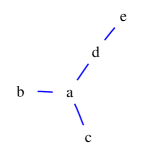
Figure 1: A toy tree model. The related itemsets $\mathopen{}\left\{a,b,c,d,e,ab,ac,ad,de\right\}$ correspond to the attributes and the edges of the tree.

We can show that the Maximum Entropy distribution for $\mathcal{T}$ has the form

$$p^{*}=\prod_{\mathopen{}\left\{a,b\right\}\in\mathcal{T}}p^{*}\mathopen{}\left(a,b\right)/\prod_{a\in G}p^{*}\mathopen{}\left(a\right).$$

This is, of course, Chow-Liu tree model[chow68tree]. We define the optimal tree to be the ne that minimises the rank, that is,

$$\mathcal{T}^{*}=\underset{\mathcal{T}\text{ is a tree}}{\arg\min}{r}\mathopen{}\left(G;\mathcal{T},D\right).$$

To solve this tree let $p_{ind}$ be the independence distribution. Corollary 3.9 allows us to rewrite the rank measure as

$${r}\mathopen{}\left(G;\mathcal{T}\right)=\mathrm{KL}\mathopen{}\left(q_{D}\|p^{*}\right)=\mathrm{KL}\mathopen{}\left(q_{D}\|p_{ind}\right)-\mathrm{KL}\mathopen{}\left(p^{*}\|p_{ind}\right).$$

Note that the first term $\mathrm{KL}\mathopen{}\left(q_{D}\|p_{ind}\right)$ does not depend on $\mathcal{T}$. Hence we need to maximise the second term $\mathrm{KL}\mathopen{}\left(p^{*}\|p_{ind}\right)$. This is the mutual information of the tree and maximising this term is equivalent to finding maximum spanning tree in the mutual information graph. This can be done in polynomial time [chow68tree].

There is a deep connection between the rank ${r}\mathopen{}\left(G;\mathcal{T}\right)$ and the rank for D-trees suggested in [heikinheimo07entropy]. We can rewrite, by applying Corollary 3.9, the rank as

$${r}\mathopen{}\left(G;\mathcal{T}\right)=\mathrm{KL}\mathopen{}\left(q_{D}\|p^{*}\right)=H\mathopen{}\left(p^{*}\right)-H\mathopen{}\left(q_{G}\right).$$

The first term $H\mathopen{}\left(p^{*}\right)$ is the rank that is used in [heikinheimo07entropy]. The authors in [heikinheimo07entropy] seek patterns that have small $H\mathopen{}\left(p^{*}\right)$, that is, trees that have strong dependencies between the attributes, whereas we are interested in patterns that produce large ${r}\mathopen{}\left(G;\mathcal{T}^{*}\right)$, sets of attributes whose joint distribution cannot be explained even by the best tree model.

Our second model involves in finding a downward closed family $\mathcal{F}$ of itemsets that produces the smallest normalised rank. Note that Corollary 3.11 implies that the rank decreases when we increase the number of known itemsets. However, this does not hold for the normalised rank and we will see that, contrary to the expectations, the best model can be different than $\mathcal{A}_{G}$, the set of all sub-itemsets of $G$. In other words, knowing all sub-itemsets does not guarantee the best model but, in fact, itemsets of higher order may mislead the prediction.

Unlike with the tree models, to our knowledge, there is no polynomial algorithm for finding the optimal downward closed family. Hence, we suggest a simple greedy approach. We start from the itemsets of size $1$ and select the itemset from the negative border that minimises the rank. The itemset is added into the family and the procedure is repeat until there is no itemset that can decrease the rank. The algorithm is stated in Algorithm 1. We use $\mathcal{F}^{*}$ to denote the resulting family.

Algorithm 1 Greedy algorithm for finding the optimal downward closed family of itemsets. The input is the data set $D$ and the query itemset $G$. The output is $\mathcal{F}^{*}$ a family of itemsets that produces low rank for the itemset.

  $\mathcal{F}^{*}\Leftarrow\mathcal{I}_{G}$. {Initialise $\mathcal{F}^{*}$ with itemsets of size $1$.}

  repeat

     $Y\Leftarrow\underset{X\in\mathrm{negbord}\mathopen{}\left(\mathcal{F}^{*}\right)}{\arg\min}{nr}\mathopen{}\left(G;\mathcal{F}^{*}\cup X\right)$.

     if ${nr}\mathopen{}\left(G;\mathcal{F}^{*}\cup Y\right)<{nr}\mathopen{}\left(G;\mathcal{F}^{*}\right)$ then

        $\mathcal{F}^{*}\Leftarrow\mathcal{F}^{*}\cup Y$.

     end if

  until no more changes in $\mathcal{F}^{*}$.

3.4 Computing Rank

Corollary 3.9 allows us to rewrite the rank as a difference of two entropies

$${r}\mathopen{}\left(G\right)=\mathrm{KL}\mathopen{}\left(q_{G}\|p^{*}\right)=H\mathopen{}\left(p^{*}\right)-H\mathopen{}\left(q_{G}\right).$$

Both distributions have $\mathopen{}\left|\Omega_{G}\right|=2^{\mathopen{}\left|G\right|}$ entries. However, the distribution $q_{G}$ can have only $\mathopen{}\left|D\right|$ positive entries at maximum, hence the term $H\mathopen{}\left(q_{G}\right)$ can be computed efficiently.

The challenge in calculating the measure is to solve the Maximum Entropy distribution $p^{*}$ and calculate its entropy. This can be done in polynomial time for the independence model and for the tree models. However, in the general case solving $p^{*}$ is an NP-complete problem [tatti06complexity, cooper90complexity]; In such cases the distribution is solved using Iterative Scaling algorithm [darroch72gis, jirousek95iterative]. The algorithm consists of consecutive steps. One such step requires $O\mathopen{}\left(\mathopen{}\left|\Omega_{G}\right|\right)=O\mathopen{}\left(2^{\mathopen{}\left|G\right|}\right)$ time. Hence computing the measure requires exponential time but it is doable for itemsets of reasonable size. The summary for evaluation times is provided in Table 1.

Measure	Description	# of degrees	Evaluation time
${r}\mathopen{}\left(G;\mathcal{I}\right)$	Independence model	$2^{\mathopen{}\left|G\right|}-1-\mathopen{}\left|G\right|$	$O\mathopen{}\left(\mathopen{}\left|G\right|\right)$
${r}\mathopen{}\left(G;\mathcal{C}\right)$	Gaussian model	$2^{\mathopen{}\left|G\right|}-1-\frac{1}{2}\mathopen{}\left|G\right|\mathopen{}\left(\mathopen{}\left|G\right|+1\right)$	$O\mathopen{}\left(2^{\mathopen{}\left|G\right|}\right)$ per iter.
${r}\mathopen{}\left(G;\mathcal{A}\right)$	All subsets model	$1$	$O\mathopen{}\left(2^{\mathopen{}\left|G\right|}\right)$ per iter.
${r}\mathopen{}\left(G;\mathcal{T}^{*}\right)$	Optimal tree model	$2^{\mathopen{}\left|G\right|}-2\mathopen{}\left|G\right|$	$O\mathopen{}\left(\mathopen{}\left|G\right|^{2}\right)$
${r}\mathopen{}\left(G;\mathcal{F}^{*}\right)$	Optimal family model	$2^{\mathopen{}\left|G\right|}-1-\mathopen{}\left|\mathcal{F}\right|$	$O\mathopen{}\left(8^{\mathopen{}\left|G\right|}\right)$ per iter.

Table 1: Summary of the rank measure. The number of degrees, the third column, is used as a a parameter for $\chi^{2}$ distribution, when computing the normalised rank. The fourth column represents the evaluation times for the entropy of $p^{*}$.

The effect of pruning itemsets.

Note that in defining the measure we only use itemsets that are subsets of the query itemset $G$. This pruning guarantees that the number of entries in the distributions is $2^{\mathopen{}\left|G\right|}$ and not, at worst, $2^{K}$, where $K$ is the number of columns in the dataset. Pruning attributes is essential since solving $p^{*}$ is exponential to the number of attributes. The downside is that pruning may change the prediction as the following example demonstrates.

Example 3.13.

Assume that we have $3$ attributes, $a$, $b$, and $c$. Our known itemsets are $\mathcal{F}=\mathopen{}\left\{a,b,c,ac,bc\right\}$ and their frequencies are $\theta_{a}=\theta_{b}=\theta_{c}=\theta_{ac}=\theta_{bc}=1/2$. In other words, the attributes are indentical and correspond to a fair coin flip. Assume that we are interested in rank of $G=ab$. In this case the pruned family of itemsets is $\mathcal{F}_{G}=\mathopen{}\left\{a,b\right\}$ and the Maximum Entropy distribution is the uniform distribution. The empirical distribution is

$$\begin{split}q_{G}(a=0,b=0)=q_{G}(a=1,b=1)&=1/2\\ q_{G}(a=1,b=0)=q_{G}(a=0,b=1)&=0.\end{split}$$

The rank is then ${r}\mathopen{}\left(ab;\mathcal{F}\right)=0.69$. However, if we had used the frequencies of $ac$ and $bc$, we would have concluded that $a=b$ and that the Maximum Entropy distribution is equal to the empirical distribution, hence the rank would have been $0$.

In [tatti06projections] we investigate the effect of pruning attributes and conclude that in some cases we can remove a large portion of attributes outside $G$. However, in those cases, the family of known itemsets has many restrictions and, for instance, we cannot remove safely any attribute from the gaussian model.

4 Related Work

Traditionally, the support (frequency) of the itemset is used for ranking itemsets. Alternative measures that resemble the support are studied in [omiecinski03measure].

Our work resembles approach of [brin97beyond] in which the authors defined the significance of an itemset by comparing the distribution $q_{G}$ against the independence model. The authors used $\chi^{2}$ statistical test as a measure, that is, if $p$ is the distribution related to the independence model, the rank measure is

$$r_{b}\mathopen{}\left(G\right)=\sum_{\omega\in\Omega_{G}}\frac{\mathopen{}\left(q_{G}(\omega)-p(\omega)\right)^{2}}{p(\omega)}.$$ (1)

In [dumouchel01empirical] the authors also compare the frequency of an itemset against the independence model but in addition they use Bayes screening to smooth the values. Also, in [aggarwal98new] the authors proposed the collective strength as a measure of significance. To be more specific, we say that a transaction $\omega\in\Omega_{G}$ is good if it contains only $0$s or only $1$s. Let $p$ be the distribution related to the independence model. Then the measure is

$$r_{cs}\mathopen{}\left(G\right)=\frac{q_{G}\mathopen{}\left(\omega\text{ is good}\right)}{p\mathopen{}\left(\omega\text{ is good}\right)}\frac{p\mathopen{}\left(\omega\text{ is bad}\right)}{q_{G}\mathopen{}\left(\omega\text{ is bad}\right)}.$$ (2)

This measure obtains small values when data obeys the independence model. In a related work presented in [dong99efficient] the authors define an itemset to be interesting if its frequency increases significantly from one dataset to another. In [gallo07mini] the authors order itemsets based on their p-values. In [heikinheimo07entropy] the authors used entropy of tree models for ranking itemsets. In addition, many measures has been suggested for ranking association rules [piatetsky91rules, brin97itemsets, agrawal93mining, jaroszewicz02pruning].

The authors in [pavlov03beyond] showed empirically that Maximum Entropy model provides excellent estimates for itemsets. Rank can be used for pruning a large family of itemsets by picking the itemsets having the largest rank. Other pruning methods are proposed in [boulicaut00approximation, calders02mining, pasquier99discovering]. The authors in [webb06significant] suggest a generic framework for discovering significant rules. In addition, a relevant framework is described in [mielikainen03pattern]; the authors define a pattern ordering given an estimation algorithm and a loss function. In [noren06who] the authors use information component analysis to find patterns in a drug safety database.

5 Experiments

In this section we present our empirical results. In the first $3$ sections we explain the datasets and the setup. In our experiments we investigate the significance of itemsets, how different measures are related to each other, and the monotonicity of the ranks.

5.1 Synthetic Datasets

For the testing purposes we created two synthetic datasets. Each dataset contained $100$ attributes and $5000$ rows. The first dataset, gen-ind, was generated such that the attributes were independent. The margins were sampled uniformly from $\mathopen{}\left[0,1\right]$. In the second dataset, gen-copy, each column was a copy of the previous column corrupted by the symmetric white noise. The amount of noise, that is the probability

$$p\mathopen{}\left(a_{i}=1\mid a_{i-1}=0\right)=p\mathopen{}\left(a_{i}=0\mid a_{i-1}=1\right),$$

was selected uniformly from $\mathopen{}\left[0,1\right]$ for each column $a_{i}$, individually. The first column was generated by a coin flip. Our expectations are that in gen-ind the itemsets of size $1$ are significant and that in gen-copy the itemsets of size $2$ are significant.

5.2 Real Datasets

In our experiments we used the following real-world datasets. Data in Accidents were obtained from the Belgian “Analysis Form for Traffic Accidents” forms that is filled out by a police officer for each traffic accident that occurs with injured or deadly wounded casualties on a public road in Belgium. In total, $340\,183$ traffic accident records are included in the dataset [geurts03accidents]. The datasets POS, WebView-1 and WebView-2 were contributed by Blue Martini Software as the KDD Cup 2000 data [kohavi00bms]. POS contains several years worth of point-of-sale data from a large electronics retailer. WebView-1 and WebView-2 contain several months worth of click-stream data from two e-commerce web sites. Kosarak consists of (anonymised) click-stream data of a Hungarian on-line news portal. Retail is a retail market basket data supplied by an anonymous Belgian retail supermarket store [brijs99retail]. The dataset Paleo contains information of species fossils found in specific paleontological sites in Europe [fortelius05now], preprocessed as in [fortelius06spectral].

5.3 Setup for the Experiments

In this section we will describe how we conducted our experiments. We reduced the largest datasets by selecting the first $10000$ rows and $200$ most frequent attributes. From each dataset we computed all almost non-derivable itemsets. By almost non-derivable we mean that the difference between the upper bound and the lower bound of a given itemset, say $G$, is at least $n$ transactions. In other words, if we know the frequencies of all sub-itemsets of $G$, then we cannot predict the frequency of $G$ within $n$ transactions. If $n=0$, then an itemset is non-derivable. It is known that the family of almost non-derivable itemsets is anti-monotonic [calders02mining, Lemma 3.1]. A reason to use almost non-derivable itemsets instead of frequent itemsets is the statement of Theorem 3.4, that is, ${r}\mathopen{}\left(G;\mathcal{A}\right)=0$ if the itemset is derivable. The other reason is that we want to study how the measure behaves for infrequent itemsets.

To keep the sizes of the obtained families within reasonable bounds we used different thresholds for different datasets: For gen-ind, Retail and WebView-2 we set $n=5$. For POS the threshold $n$ was set to $10$ and for gen-copy and Accidents $n$ was set to $100$. For the rest of the datasets we set $n=0$, that is, we mined all non-derivable itemsets from these datasets.

For each itemset from the obtained itemsets we queried the following measures:

• Frequency.

• Normalised rank measures ${nr}\mathopen{}\left(G;\mathcal{I}\right)$, ${nr}\mathopen{}\left(G;\mathcal{C}\right)$, ${nr}\mathopen{}\left(G;\mathcal{A}\right)$, ${nr}\mathopen{}\left(G;\mathcal{T}^{*}\right)$, ${nr}\mathopen{}\left(G;\mathcal{F}^{*}\right)$.

• Measures discussed in Section 4: A $\chi^{2}$ test $r_{b}\mathopen{}\left(G\right)$ defined in Eq. 1 and a collective strength $r_{cs}\mathopen{}\left(G\right)$ defined in Eq. 2.

The evaluation times and the sizes of the query families are given in Table 2.

				Evaluation times
Data	$n$	# of $G$	$\max\mathopen{}\left|G\right|$	${nr}\mathopen{}\left(G;\mathcal{I}\right)$	${nr}\mathopen{}\left(G;\mathcal{C}\right)$	${nr}\mathopen{}\left(G;\mathcal{A}\right)$	${nr}\mathopen{}\left(G;\mathcal{T}^{*}\right)$	${nr}\mathopen{}\left(G;\mathcal{F}^{*}\right)$
gen-ind	$5$	$156699$	$6$	$2s$	$52s$	$29min$	$2s$	$11min$
gen-copy	$100$	$111487$	$4$	$0s$	$12s$	$57s$	$0s$	$1min$
Accidents	$100$	$354399$	$6$	$2s$	$1min$	$19min$	$3s$	$108min$
Kosarak	$5$	$223734$	$5$	$1s$	$4s$	$9s$	$0s$	$47s$
Paleo	$0$	$166903$	$5$	$0s$	$8s$	$35s$	$0s$	$2min$
POS	$10$	$246640$	$6$	$1s$	$8s$	$27s$	$1s$	$5min$
Retail	$0$	$818813$	$6$	$3s$	$19s$	$49s$	$4s$	$4min$
WebView-1	$5$	$226313$	$5$	$1s$	$5s$	$8s$	$1s$	$39s$
WebView-2	$0$	$715398$	$6$	$3s$	$27s$	$2min$	$4s$	$11min$

Table 2: The evaluation times and the sizes of the query families. The second column is the threshold used in mining almost non-derivable itemsets. The fourth column is the maximal size of a query itemset. The evaluation time does not include the time spent mining itemsets.

5.4 Significant Itemsets

Our first experiment is to study how many of the itemsets are significant. We did this by comparing the our rank measures with risk level 0.05. The results are given in Tables 3–5. We also provide a typical example of box plots in Figure 2.

	itemset size
Data	1	2	3	4	5	6	All
gen-ind	$.92$	$.05$	$.04$	$.03$	$.02$	$.01$	$.03$
gen-copy	$.08$	$.14$	$.24$	$.03$	–	–	$.07$
Accidents	$.99$	$.60$	$.95$	$1$	$1$	$1$	$.97$
Kosarak	$1$	$.62$	$.99$	$1$	$1$	–	$.96$
Paleo	$1$	$.30$	$.81$	$.99$	$1$	–	$.88$
POS	$1$	$.45$	$.99$	$1$	$1$	$1$	$.95$
Retail	$1$	$.14$	$.30$	$.93$	$1$	$1$	$.45$
WebView-1	$1$	$.70$	$1$	$1$	$1$	–	$.97$
WebView-2	$1$	$.20$	$.69$	$1$	$1$	$1$	$.85$

Table 3: The percentages of significant itemsets according to ${nr}\mathopen{}\left(G;\mathcal{I}\right)$. Each entry is a fraction of itemsets of specific size calculated from a specific dataset. Significance is measured using $\chi^{2}$ distribution with $0.05$ risk level.

	${nr}\mathopen{}\left(G;\mathcal{C}\right)$, itemset size								${nr}\mathopen{}\left(G;\mathcal{A}\right)$, itemset size
Data	1	2	3	4	5	6	All		1	2	3	4	5	6	All
gen-ind	$.92$	$.05$	$.06$	$.05$	$.04$	$.03$	$.05$		$.92$	$.05$	$.06$	$.06$	$.06$	$.06$	$.06$
gen-copy	$.08$	$.14$	$.06$	$.03$	–	–	$.03$		$.08$	$.14$	$.06$	$.05$	–	–	$.05$
Accidents	$.99$	$.60$	$.21$	$.45$	$.62$	$.60$	$.45$		$.99$	$.60$	$.21$	$.07$	$.05$	$.06$	$.11$
Kosarak	$1$	$.62$	$.32$	$.50$	$.38$	–	$.37$		$1$	$.62$	$.32$	$.10$	$.04$	–	$.33$
Paleo	$1$	$.30$	$.12$	$.15$	$.21$	–	$.15$		$1$	$.30$	$.12$	$.21$	$.64$	–	$.18$
POS	$1$	$.45$	$.09$	$.21$	$.43$	$.66$	$.17$		$1$	$.45$	$.09$	$.06$	$.07$	$.05$	$.11$
Retail	$1$	$.14$	$.04$	$.08$	$.12$	$.38$	$.05$		$1$	$.14$	$.04$	$.15$	$.27$	$.25$	$.07$
WebView-1	$1$	$.70$	$.48$	$.32$	$.52$	–	$.48$		$1$	$.70$	$.48$	$.09$	$.07$	–	$.45$
WebView-2	$1$	$.20$	$.11$	$.20$	$.88$	$1$	$.17$		$1$	$.20$	$.11$	$.16$	$.36$	$.48$	$.15$

Table 4: The percentages of significant itemsets according to ${nr}\mathopen{}\left(G;\mathcal{C}\right)$ and ${nr}\mathopen{}\left(G;\mathcal{A}\right)$. Each entry is a fraction of itemsets of specific size calculated from a specific dataset. Significance is measured using $\chi^{2}$ distribution with $0.05$ risk level.

	${nr}\mathopen{}\left(G;\mathcal{T}^{*}\right)$, itemset size								${nr}\mathopen{}\left(G;\mathcal{F}^{*}\right)$, itemset size
Data	1	2	3	4	5	6	All		1	2	3	4	5	6	All
gen-ind	$.92$	$.05$	$.02$	$.01$	$.01$	$0$	$.01$		$.92$	$.05$	$.01$	$.01$	$0$	$0$	$.01$
gen-copy	$.08$	$.14$	$.02$	$0$	–	–	$.01$		$.08$	$.14$	$.01$	$0$	–	–	$.01$
Accidents	$.99$	$.60$	$.40$	$.80$	$.95$	$.97$	$.75$		$.99$	$.60$	$.18$	$.12$	$.13$	$.02$	$.15$
Kosarak	$1$	$.62$	$.80$	$.94$	$1$	–	$.80$		$1$	$.62$	$.32$	$.05$	$.03$	–	$.32$
Paleo	$1$	$.30$	$.10$	$.35$	$.81$	–	$.24$		$1$	$.30$	$.06$	$.05$	$.04$	–	$.07$
POS	$1$	$.45$	$.47$	$.99$	$1$	$1$	$.65$		$1$	$.45$	$.08$	$.02$	$.02$	$0$	$.09$
Retail	$1$	$.14$	$.03$	$.18$	$.78$	$1$	$.07$		$1$	$.14$	$.01$	$.02$	$.02$	$.13$	$.02$
WebView-1	$1$	$.70$	$.83$	$1$	$1$	–	$.84$		$1$	$.70$	$.46$	$.07$	$.30$	–	$.43$
WebView-2	$1$	$.20$	$.11$	$.57$	$1$	$1$	$.37$		$1$	$.20$	$.06$	$.03$	$.14$	$.44$	$.05$

Table 5: The percentages of significant itemsets according to ${nr}\mathopen{}\left(G;\mathcal{T}^{*}\right)$ and ${nr}\mathopen{}\left(G;\mathcal{F}^{*}\right)$. Each entry is a fraction of itemsets of specific size calculated from a specific dataset. Significance is measured using $\chi^{2}$ distribution with $0.05$ risk level.

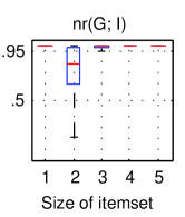
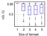
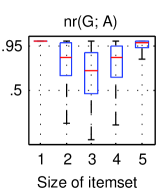
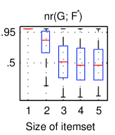
Figure 2: Box plots of the rank measures computed from Paleo.

Let us first study gen-ind, a synthetic dataset with independent columns. We see from Table 3 that according to ${nr}\mathopen{}\left(G;\mathcal{I}\right)$ a large portion of itemsets of size $1$ are significant but only a small portion of itemsets having size larger than $1$ is significant. This is an expected result since the frequencies obey the independence model. In Tables 4 we have similar results for ${nr}\mathopen{}\left(G;\mathcal{C}\right)$ and for ${nr}\mathopen{}\left(G;\mathcal{A}\right)$. However, the values of ${nr}\mathopen{}\left(G;\mathcal{C}\right)$ and for ${nr}\mathopen{}\left(G;\mathcal{A}\right)$ tend to be larger than the values of ${nr}\mathopen{}\left(G;\mathcal{I}\right)$. The reason for this is a type of overlearning: Since the frequencies of itemsets are calculated from the datasets, they are imprecise. Hence, the itemsets with larger size mislead us during prediction, because the resulting Maximum Entropy distribution is not an independent model (although close to one).

Let us continue by studying gen-copy, a synthetic data in which an attribute is a noisy copy of the previous attribute. We see that ${nr}\mathopen{}\left(G;\mathcal{T}^{*}\right)$ tends to have smaller ranks than ${nr}\mathopen{}\left(G;\mathcal{I}\right)$ when $G$ has size $3$. The reason for this is that, unlike with gen-ind, the independence model cannot explain the dataset. However, when we predict using also the itemsets of size $2$, the prediction becomes more accurate. The measures ${nr}\mathopen{}\left(G;\mathcal{C}\right)$ and ${nr}\mathopen{}\left(G;\mathcal{A}\right)$ also produce small ranks, however, these ranks tend to be slightly larger than the ranks of ${nr}\mathopen{}\left(G;\mathcal{T}^{*}\right)$.

We turn our attention to real datasets. We see that for these datasets the independence model is too strict: According to ${nr}\mathopen{}\left(G;\mathcal{I}\right)$ almost all itemsets are significant: The results change drastically, when we use richer models. According to ${nr}\mathopen{}\left(G;\mathcal{C}\right)$ or ${nr}\mathopen{}\left(G;\mathcal{A}\right)$ only $5\%$–$50\%$ of the itemsets are significant, depending on the dataset. Similar overfitting that occurred with gen-ind also occurs in some but not all real datasets (see Figure 2). For instance, in Retail ${nr}\mathopen{}\left(G;\mathcal{A}\right)$ tends to produce higher values than ${nr}\mathopen{}\left(G;\mathcal{C}\right)$ but not in POS.

5.5 The Effect of the Known Itemsets

We continued our experiments by comparing the measures ${nr}\mathopen{}\left(G;\mathcal{I}\right)$, ${nr}\mathopen{}\left(G;\mathcal{C}\right)$, ${nr}\mathopen{}\left(G;\mathcal{A}\right)$, ${nr}\mathopen{}\left(G;\mathcal{T}^{*}\right)$, and ${nr}\mathopen{}\left(G;\mathcal{F}^{*}\right)$ against each other. This was done by calculating the correlations between the rank measures. The results are given in Tables 6 and 7.

	${nr}\mathopen{}\left(G;\mathcal{I}\right)$	${nr}\mathopen{}\left(G;\mathcal{I}\right)$	${nr}\mathopen{}\left(G;\mathcal{C}\right)$
	vs.	vs.	vs.
Data	${nr}\mathopen{}\left(G;\mathcal{C}\right)$	${nr}\mathopen{}\left(G;\mathcal{A}\right)$	${nr}\mathopen{}\left(G;\mathcal{A}\right)$
gen-ind	$.74$	$.26$	$.39$
gen-copy	$.52$	$.28$	$.53$
Accidents	$.17$	$.07$	$.37$
Kosarak	$.14$	$.13$	$.90$
Paleo	$.16$	$.22$	$.67$
POS	$.12$	$.10$	$.77$
Retail	$.62$	$.67$	$.88$
WebView-1	$.14$	$.12$	$.88$
WebView-2	$.43$	$.51$	$.68$

Table 6: Correlations between the measures ${nr}\mathopen{}\left(G;\mathcal{I}\right)$, ${nr}\mathopen{}\left(G;\mathcal{C}\right)$, and ${nr}\mathopen{}\left(G;\mathcal{A}\right)$.

	${nr}\mathopen{}\left(G;\mathcal{T}^{*}\right)$ vs.				${nr}\mathopen{}\left(G;\mathcal{F}^{*}\right)$ vs.
Data	${nr}\mathopen{}\left(G;\mathcal{I}\right)$	${nr}\mathopen{}\left(G;\mathcal{C}\right)$	${nr}\mathopen{}\left(G;\mathcal{A}\right)$		${nr}\mathopen{}\left(G;\mathcal{I}\right)$	${nr}\mathopen{}\left(G;\mathcal{C}\right)$	${nr}\mathopen{}\left(G;\mathcal{A}\right)$	${nr}\mathopen{}\left(G;\mathcal{T}^{*}\right)$
gen-ind	$.81$	$.94$	$.37$		$.81$	$.91$	$.36$	$.98$
gen-copy	$.62$	$.92$	$.49$		$.64$	$.89$	$.49$	$.97$
Accidents	$.34$	$.57$	$.20$		$.07$	$.58$	$.54$	$.29$
Kosarak	$.41$	$.41$	$.36$		$.13$	$.85$	$.93$	$.46$
Paleo	$.35$	$.64$	$.47$		$.16$	$.84$	$.67$	$.62$
POS	$.42$	$.34$	$.28$		$.05$	$.72$	$.84$	$.21$
Retail	$.66$	$.82$	$.82$		$.59$	$.92$	$.84$	$.86$
WebView-1	$.56$	$.29$	$.24$		$.12$	$.86$	$.93$	$.28$
WebView-2	$.59$	$.62$	$.65$		$.34$	$.77$	$.72$	$.54$

Table 7: Correlations between the flexible measures ${nr}\mathopen{}\left(G;\mathcal{T}^{*}\right)$ and ${nr}\mathopen{}\left(G;\mathcal{F}^{*}\right)$ and the measures ${nr}\mathopen{}\left(G;\mathcal{I}\right)$, ${nr}\mathopen{}\left(G;\mathcal{C}\right)$, and ${nr}\mathopen{}\left(G;\mathcal{A}\right)$.

From the results we see that all correlations are positive. For the real datasets the correlations between ${nr}\mathopen{}\left(G;\mathcal{C}\right)$ and ${nr}\mathopen{}\left(G;\mathcal{A}\right)$ are systematically higher than the correlations between ${nr}\mathopen{}\left(G;\mathcal{I}\right)$ and ${nr}\mathopen{}\left(G;\mathcal{A}\right)$ or between ${nr}\mathopen{}\left(G;\mathcal{C}\right)$ and ${nr}\mathopen{}\left(G;\mathcal{A}\right)$. This suggests that ${nr}\mathopen{}\left(G;\mathcal{I}\right)$ produces different ranks whereas ${nr}\mathopen{}\left(G;\mathcal{C}\right)$ and ${nr}\mathopen{}\left(G;\mathcal{A}\right)$ are more similar. This supports the behaviour we have seen in Section 5.4.

The measure ${nr}\mathopen{}\left(G;\mathcal{F}^{*}\right)$ correlate more with ${nr}\mathopen{}\left(G;\mathcal{A}\right)$ and ${nr}\mathopen{}\left(G;\mathcal{C}\right)$ than with ${nr}\mathopen{}\left(G;\mathcal{I}\right)$. The correlation between ${nr}\mathopen{}\left(G;\mathcal{F}^{*}\right)$ and ${nr}\mathopen{}\left(G;\mathcal{T}^{*}\right)$ is somewhat weaker but it is stronger than the correlation between ${nr}\mathopen{}\left(G;\mathcal{F}^{*}\right)$ and ${nr}\mathopen{}\left(G;\mathcal{I}\right)$.

5.6 Flexible Models

Our next goal is to compare the flexible measures ${nr}\mathopen{}\left(G;\mathcal{T}^{*}\right)$ and ${nr}\mathopen{}\left(G;\mathcal{F}^{*}\right)$ against the rest of the measures. From Table 5 we see that ${nr}\mathopen{}\left(G;\mathcal{F}^{*}\right)$ tend to produce the smallest amount of significant itemsets whereas the ${nr}\mathopen{}\left(G;\mathcal{T}^{*}\right)$ produces large ranks, especially for queries with many attributes.

We calculated the number of queries in which ${nr}\mathopen{}\left(G;\mathcal{T}^{*}\right)$ and ${nr}\mathopen{}\left(G;\mathcal{F}^{*}\right)$ produce smaller rank than the rest of the measures. Since the measures are equivalent for the queries of size $1$ and $2$, these queries were ignored. From the results given in Table 8 we see that the flexible models outperform ${nr}\mathopen{}\left(G;\mathcal{I}\right)$, however, the performance against other measure depends on the data set. For instance, ${nr}\mathopen{}\left(G;\mathcal{F}^{*}\right)$ outperform ${nr}\mathopen{}\left(G;\mathcal{C}\right)$ and ${nr}\mathopen{}\left(G;\mathcal{A}\right)$ in Retail but produces larger ranks in Kosarak. This suggests that the greedy algorithm sometimes fails to find the optimal family $\mathcal{F}^{*}$.

	${{nr}\mathopen{}\left(G;\mathcal{T}^{*}\right)}\leq$				${{nr}\mathopen{}\left(G;\mathcal{F}^{*}\right)}\leq$
Data	${nr}\mathopen{}\left(G;\mathcal{I}\right)$	${nr}\mathopen{}\left(G;\mathcal{C}\right)$	${nr}\mathopen{}\left(G;\mathcal{A}\right)$		${nr}\mathopen{}\left(G;\mathcal{I}\right)$	${nr}\mathopen{}\left(G;\mathcal{C}\right)$	${nr}\mathopen{}\left(G;\mathcal{A}\right)$	${nr}\mathopen{}\left(G;\mathcal{T}^{*}\right)$
gen-ind	$.84$	$.97$	$.78$		$1$	$.99$	$.81$	$.95$
gen-copy	$.79$	$.96$	$.82$		$1$	$.99$	$.86$	$.99$
Accidents	$1$	$.16$	$.13$		$1$	$.94$	$.66$	$.95$
Kosarak	$1$	$.08$	$.08$		$1$	$.38$	$.36$	$.96$
Paleo	$.99$	$.47$	$.58$		$1$	$.91$	$.85$	$.86$
POS	$1$	$.12$	$.12$		$1$	$.65$	$.62$	$.90$
Retail	$.92$	$.77$	$.80$		$1$	$.94$	$.92$	$.62$
WebView-1	$1$	$.19$	$.19$		$1$	$.52$	$.49$	$.93$
WebView-2	$.99$	$.37$	$.46$		$1$	$.89$	$.87$	$.79$

Table 8: Percentages of queries in which the flexible measures ${nr}\mathopen{}\left(G;\mathcal{T}^{*}\right)$ and ${nr}\mathopen{}\left(G;\mathcal{F}^{*}\right)$ outperform the other rank measures. Queries only of size $3$ or larger were considered.

We studied the sizes of itemsets occurring in $\mathcal{F}^{*}$, the family of known itemsets in ${nr}\mathopen{}\left(G;\mathcal{F}^{*}\right)$. To be more precise, let $\mathcal{F}^{*}_{G}$ be the family of known itemsets for the query $G$. Let $L$ be the size of itemsets we are interested in. We define the ratio $r_{L}$ to be

$$r_{L}=\frac{\sum_{G}\mathopen{}\left|\mathopen{}\left\{X\in\mathcal{F}^{*}_{G};\mathopen{}\left|X\right|=L\right\}\right|}{\sum_{G}{\mathopen{}\left|G\right|\choose L}},$$

that is, the number of itemset of size $L$ occurring in $\mathcal{F}^{*}$ divided by the maximum number of occurrences. The ratios $r_{L}$ are given in Table 9. We see that the itemsets of size $2$ and $3$ are frequently used, however, the itemsets of larger size are rarely used.

	Ratio of used itemsets
Data	2	3	4	5
gen-ind	$.35$	$.01$	$0$	$0$
gen-copy	$.36$	$.01$	–	–
Accidents	$.87$	$.36$	$.02$	$0$
Kosarak	$.95$	$.49$	$.01$	–
Paleo	$.74$	$.16$	$0$	–
POS	$.96$	$.47$	$.01$	$0$
Retail	$.62$	$.13$	$0$	$0$
WebView-1	$.93$	$.44$	$0$	–
WebView-2	$.81$	$.26$	$.07$	$0$

Table 9: Number of itemsets occurring in $\mathcal{F}^{*}$, the family of known itemsets in ${r}\mathopen{}\left(G;\mathcal{F}^{*}\right)$, normalised by the maximum number of possible occurrences. Each column represent itemsets of specific size.

5.7 Rank vs. Other Methods

We compared our measures against the other ranking methods described in Section 5.3. Namely, we calculated the correlations of ${nr}\mathopen{}\left(G;\mathcal{I}\right)$, ${nr}\mathopen{}\left(G;\mathcal{C}\right)$, ${nr}\mathopen{}\left(G;\mathcal{A}\right)$, ${nr}\mathopen{}\left(G;\mathcal{T}^{*}\right)$, and ${nr}\mathopen{}\left(G;\mathcal{F}^{*}\right)$ against the frequency of $G$, $r_{b}\mathopen{}\left(G\right)$, the $\chi^{2}$ test for independency, and $r_{cs}\mathopen{}\left(G\right)$, the collective strength of the itemset $G$. The results are presented in Tables 10 and 11. We also studied the relationships by plotting our measures as functions of the aforementioned approaches and such examples are given in Figure 3.

	${nr}\mathopen{}\left(G;\mathcal{I}\right)$ vs.			${nr}\mathopen{}\left(G;\mathcal{C}\right)$ vs.			${nr}\mathopen{}\left(G;\mathcal{A}\right)$ vs.
Data	freq.	$r_{b}\mathopen{}\left(G\right)$	$r_{cs}\mathopen{}\left(G\right)$	freq.	$r_{b}\mathopen{}\left(G\right)$	$r_{cs}\mathopen{}\left(G\right)$	freq.	$r_{b}\mathopen{}\left(G\right)$	$r_{cs}\mathopen{}\left(G\right)$
gen-ind	$.06$	$.99$	$-.01$	$.03$	$.72$	$-.01$	$0$	$.25$	$0$
gen-copy	$.15$	$1$	$.02$	$.07$	$.52$	$.02$	$.01$	$.27$	$.01$
Accidents	$.01$	$1$	$.02$	$-.01$	$.17$	$.05$	$.03$	$.07$	$.01$
Kosarak	$.01$	$.98$	$.20$	$.01$	$.14$	$.27$	$0$	$.13$	$.21$
Paleo	$.18$	$.95$	$.39$	$.01$	$.15$	$.10$	$-.03$	$.20$	$.03$
POS	$.05$	$.99$	$.22$	$.09$	$.12$	$.20$	$.07$	$.10$	$0$
Retail	$.04$	$.97$	$.31$	$.05$	$.57$	$.17$	$.05$	$.61$	$.25$
WebView-1	$.06$	$.98$	$.19$	$.07$	$.15$	$-.29$	$.05$	$.13$	$-.32$
WebView-2	$.12$	$.96$	$.33$	$.17$	$.36$	$.39$	$.12$	$.43$	$.25$

Table 10: Correlations between the rank measures ${nr}\mathopen{}\left(G;\mathcal{I}\right)$, ${nr}\mathopen{}\left(G;\mathcal{C}\right)$, and ${nr}\mathopen{}\left(G;\mathcal{A}\right)$ and the base measures: the frequency of $G$, $r_{b}\mathopen{}\left(G\right)$, the $\chi^{2}$ test for independency, and $r_{cs}\mathopen{}\left(G\right)$, the collective strength of the itemset $G$.

	${nr}\mathopen{}\left(G;\mathcal{T}^{*}\right)$ vs.			${nr}\mathopen{}\left(G;\mathcal{F}^{*}\right)$ vs.
Data	freq.	$r_{b}\mathopen{}\left(G\right)$	$r_{cs}\mathopen{}\left(G\right)$	freq.	$r_{b}\mathopen{}\left(G\right)$	$r_{cs}\mathopen{}\left(G\right)$
gen-ind	$.07$	$.79$	$-.01$	$.06$	$.79$	$-.01$
gen-copy	$.16$	$.62$	$.03$	$.16$	$.64$	$.03$
Accidents	$-.02$	$.33$	$.04$	$.04$	$.07$	$.01$
Kosarak	$.01$	$.39$	$.32$	$0$	$.13$	$.25$
Paleo	$.24$	$.28$	$.44$	$.09$	$.12$	$.03$
POS	$.12$	$.41$	$.37$	$.07$	$.05$	$-.23$
Retail	$.06$	$.58$	$.31$	$.06$	$.53$	$.14$
WebView-1	$.11$	$.55$	$.16$	$.04$	$.13$	$-.35$
WebView-2	$.20$	$.49$	$.46$	$.16$	$.28$	$.14$

Table 11: Correlations between the rank measures ${nr}\mathopen{}\left(G;\mathcal{T}^{*}\right)$ and ${nr}\mathopen{}\left(G;\mathcal{F}^{*}\right)$ and the base measures: the frequency of $G$, $r_{b}\mathopen{}\left(G\right)$, the $\chi^{2}$ test for independency, and $r_{cs}\mathopen{}\left(G\right)$, the collective strength of the itemset $G$.

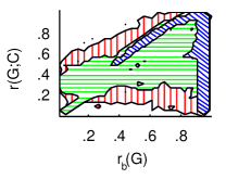
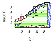
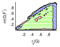
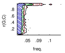
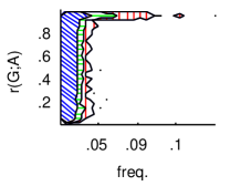
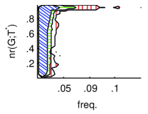
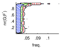
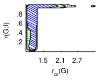
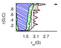
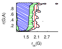
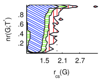
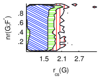
Figure 3: Ranks as functions of the base measures. The plots are calculated from Paleo dataset.

Our first observation is that ${nr}\mathopen{}\left(G;\mathcal{I}\right)$ correlates strongly with $r_{b}\mathopen{}\left(G\right)$. This is an expected result since both test the independency of attributes inside the itemsets and also because ${nr}\mathopen{}\left(G;\mathcal{I}\right)$ is asymptotically a $\chi^{2}$ test (see Theorem 3.7). There is some correlation between $r_{b}\mathopen{}\left(G\right)$ and the rest of the measures although this correlation is much weaker compared to ${nr}\mathopen{}\left(G;\mathcal{I}\right)$.

Apart from WebView-2, there is little correlation between the measures and the frequency.

The correlation between the measures and the collective strength $r_{cs}\mathopen{}\left(G\right)$ exists but varies depending on the method and the dataset. The strongest correlations are obtained when $r_{cs}\mathopen{}\left(G\right)$ is compared against ${nr}\mathopen{}\left(G;\mathcal{I}\right)$ or ${nr}\mathopen{}\left(G;\mathcal{T}^{*}\right)$. The dependency between ${nr}\mathopen{}\left(G;\mathcal{I}\right)$ and $r_{cs}\mathopen{}\left(G\right)$ is a natural result since $r_{cs}\mathopen{}\left(G\right)$ produces small values when attributes are independent.

5.8 Monotonicity of Rank

In this section we investigate the relationship between the rank of an itemset and the ranks of its sub-itemsets. Namely, we tested whether the measures are monotonic, that is, whether ${nr}\mathopen{}\left(G;\mathcal{F}\right)\geq{nr}\mathopen{}\left(H;\mathcal{F}\right)$ for all $H\subset G$. We deliberately ignored sub-itemsets having size $1$ since they all have very high rank. We also tested whether the measures are anti-monotonic, that is, decreasing w.r.t. set inclusion.

	${nr}\mathopen{}\left(G;\mathcal{I}\right)$					${nr}\mathopen{}\left(G;\mathcal{C}\right)$					${nr}\mathopen{}\left(G;\mathcal{A}\right)$
Data	3	4	5	6	All	3	4	5	6	All	3	4	5	6	All
gen-ind	$.09$	$.02$	$.01$	$0$	$.03$	$.27$	$.03$	$.01$	$0$	$.05$	$.27$	$.11$	$.06$	$.03$	$.11$
gen-copy	$.15$	$.01$	–	–	$.04$	$.20$	$.02$	–	–	$.05$	$.20$	$.10$	–	–	$.12$
Accidents	$.78$	$.92$	$.97$	$.99$	$.90$	$.01$	$.02$	$.02$	$0$	$.02$	$.01$	$0$	$0$	$0$	$0$
Kosarak	$.93$	$.98$	$1$	–	$.93$	$0$	$0$	$0$	–	$0$	$0$	$0$	$0$	–	$0$
Paleo	$.40$	$.61$	$.84$	–	$.51$	$.04$	$0$	$0$	–	$.02$	$.04$	$0$	$0$	–	$.02$
POS	$.87$	$1$	$1$	$1$	$.92$	$0$	$0$	$.01$	$0$	$0$	$0$	$0$	$0$	$0$	$0$
Retail	$.11$	$.42$	$.92$	$1$	$.19$	$.04$	$0$	$0$	$0$	$.03$	$.04$	$.02$	$0$	$0$	$.04$
WebView-1	$.98$	$1$	$1$	–	$.98$	$.04$	$0$	$0$	–	$.04$	$.04$	$0$	$0$	–	$.04$
WebView-2	$.39$	$.88$	$1$	$1$	$.67$	$.04$	$0$	$.08$	$1$	$.02$	$.04$	$0$	$0$	$0$	$.02$

Table 12: Percentages of itemsets satisfying the property of monotonicity. The itemset $G$ satisfies the property if ${nr}\mathopen{}\left(G;\mathcal{F}\right)\geq{nr}\mathopen{}\left(H;\mathcal{F}\right)$ for all $H\subset G$ such that $\mathopen{}\left|H\right|\geq 2$.

	${nr}\mathopen{}\left(G;\mathcal{T}^{*}\right)$					${nr}\mathopen{}\left(G;\mathcal{F}^{*}\right)$
Data	3	4	5	6	All	3	4	5	6	All
gen-ind	$.13$	$.01$	$0$	$0$	$.02$	$.07$	$.01$	$0$	$0$	$.02$
gen-copy	$.10$	$.01$	–	–	$.02$	$.05$	$.01$	–	–	$.02$
Accidents	$.02$	$.13$	$.35$	$.47$	$.17$	$.01$	$0$	$0$	$0$	$0$
Kosarak	$0$	$.26$	$.32$	–	$.03$	$0$	$0$	$0$	–	$0$
Paleo	$.02$	$0$	$0$	–	$.01$	$.02$	$0$	$0$	–	$.01$
POS	$0$	$.23$	$.97$	$1$	$.11$	$0$	$0$	$0$	$0$	$0$
Retail	$.03$	$0$	$.14$	$1$	$.02$	$.02$	$0$	$0$	$0$	$.02$
WebView-1	$.04$	$.07$	$.89$	–	$.05$	$.03$	$0$	$0$	–	$.03$
WebView-2	$.03$	$.02$	$.72$	$1$	$.04$	$.03$	$0$	$0$	$0$	$.01$

Table 13: Percentages of itemsets satisfying the property of monotonicity. The itemset $G$ satisfies the property if ${nr}\mathopen{}\left(G;\mathcal{F}\right)\geq{nr}\mathopen{}\left(H;\mathcal{F}\right)$ for all $H\subset G$ such that $\mathopen{}\left|H\right|\geq 2$.

	${nr}\mathopen{}\left(G;\mathcal{I}\right)$					${nr}\mathopen{}\left(G;\mathcal{C}\right)$					${nr}\mathopen{}\left(G;\mathcal{A}\right)$
Data	3	4	5	6	All	3	4	5	6	All	3	4	5	6	All
gen-ind	$.21$	$.07$	$.03$	$.02$	$.07$	$.25$	$.07$	$.03$	$.01$	$.07$	$.25$	$.08$	$.02$	$.01$	$.07$
gen-copy	$.15$	$.06$	–	–	$.08$	$.25$	$.08$	–	–	$.11$	$.25$	$.07$	–	–	$.10$
Accidents	$.03$	$0$	$0$	$0$	$.01$	$.62$	$.04$	$0$	$0$	$.16$	$.62$	$.21$	$.05$	$.02$	$.26$
Kosarak	$.02$	$.06$	$0$	–	$.02$	$.93$	$.03$	$.01$	–	$.83$	$.93$	$.33$	$.08$	–	$.86$
Paleo	$.02$	$0$	$0$	–	$.01$	$.43$	$.04$	$0$	–	$.22$	$.43$	$.07$	$0$	–	$.23$
POS	$.01$	$.01$	$.04$	$.23$	$.01$	$.87$	$.07$	$0$	$0$	$.57$	$.87$	$.18$	$.06$	$.09$	$.61$
Retail	$.17$	$0$	$0$	$0$	$.13$	$.38$	$.05$	$.01$	$0$	$.30$	$.38$	$.03$	$.01$	$0$	$.29$
WebView-1	$0$	$0$	$0$	–	$0$	$.69$	$.11$	$0$	–	$.62$	$.69$	$.39$	$.15$	–	$.66$
WebView-2	$.07$	$.01$	$.14$	$.96$	$.04$	$.48$	$.06$	$0$	$0$	$.24$	$.48$	$.06$	$.07$	$.04$	$.25$

Table 14: Percentages of itemsets satisfying the property of anti-monotonicity. The itemset $G$ satisfies the property if ${nr}\mathopen{}\left(G;\mathcal{F}\right)\leq{nr}\mathopen{}\left(H;\mathcal{F}\right)$ for all $H\subset G$ such that $\mathopen{}\left|H\right|\geq 2$.

	${nr}\mathopen{}\left(G;\mathcal{T}^{*}\right)$					${nr}\mathopen{}\left(G;\mathcal{F}^{*}\right)$
Data	3	4	5	6	All	3	4	5	6	All
gen-ind	$.45$	$.16$	$.06$	$.02$	$.15$	$.53$	$.16$	$.05$	$.01$	$.15$
gen-copy	$.43$	$.18$	–	–	$.22$	$.51$	$.17$	–	–	$.23$
Accidents	$.58$	$.01$	$0$	$0$	$.13$	$.69$	$.29$	$.07$	$.02$	$.32$
Kosarak	$.91$	$0$	$0$	–	$.81$	$.95$	$.50$	$.07$	–	$.90$
Paleo	$.52$	$.02$	$0$	–	$.25$	$.56$	$.15$	$.01$	–	$.34$
POS	$.88$	$0$	$0$	$0$	$.56$	$.90$	$.47$	$.13$	$0$	$.73$
Retail	$.72$	$.02$	$0$	$0$	$.55$	$.75$	$.13$	$.03$	$0$	$.60$
WebView-1	$.62$	$0$	$0$	–	$.55$	$.70$	$.56$	$.22$	–	$.68$
WebView-2	$.69$	$.01$	$0$	$0$	$.31$	$.71$	$.23$	$.06$	$0$	$.44$

Table 15: Percentages of itemsets satisfying the property of anti-monotonicity. The itemset $G$ satisfies the property if ${nr}\mathopen{}\left(G;\mathcal{F}\right)\leq{nr}\mathopen{}\left(H;\mathcal{F}\right)$ for all $H\subset G$ such that $\mathopen{}\left|H\right|\geq 2$.

From the results given in Tables 12–15 our first observation is that ${nr}\mathopen{}\left(G;\mathcal{I}\right)$ are increasing for real datasets but not for the synthetic datasets. The raw values of ${nr}\mathopen{}\left(G;\mathcal{I}\right)$ are indeed increasing but this does not hold for the P-values since the number of degrees varies. The measure ${nr}\mathopen{}\left(G;\mathcal{T}^{*}\right)$ tends also be monotonic but not as much as ${nr}\mathopen{}\left(G;\mathcal{I}\right)$. On the contrary, ${nr}\mathopen{}\left(G;\mathcal{C}\right)$, ${nr}\mathopen{}\left(G;\mathcal{A}\right)$, and ${nr}\mathopen{}\left(G;\mathcal{F}^{*}\right)$ are increasing for extremely few itemsets.

Table 14 suggests that ${nr}\mathopen{}\left(G;\mathcal{C}\right)$, ${nr}\mathopen{}\left(G;\mathcal{A}\right)$, and ${nr}\mathopen{}\left(G;\mathcal{F}^{*}\right)$ satisfies the anti-monotonicity to some degree. Measures ${nr}\mathopen{}\left(G;\mathcal{C}\right)$ and ${nr}\mathopen{}\left(G;\mathcal{A}\right)$ are anti-monotonic for relatively high percentage of itemsets of size $3$. Among itemsets of size $4$, ${nr}\mathopen{}\left(G;\mathcal{F}^{*}\right)$ satisfies the property of anti-monotonicity for a slightly larger portion of itemsets than ${nr}\mathopen{}\left(G;\mathcal{A}\right)$ that, in turn, is anti-monotonic in more queries than ${nr}\mathopen{}\left(G;\mathcal{C}\right)$.

6 Conclusions

We have given a definition of a measure for ranking itemsets. The idea is to predict the frequency of an itemset from the frequencies of its sub-itemsets and measure the deviation between the actual frequency and the prediction. The more the itemset deviates from the prediction, the more it is significant. We estimated the frequencies using Maximum Entropy and we used Kullback-Leibler divergence to measure the deviation. In the general case, the measure can be computed in $O(2^{\mathopen{}\left|G\right|})$ time, where $\mathopen{}\left|G\right|$ is the size of the itemset needed to be ranked, however, the measures ${r}\mathopen{}\left(G;\mathcal{T}^{*}\right)$ and ${r}\mathopen{}\left(G;\mathcal{I}\right)$ can be computed in polynomial time.

We introduced two flexible rank measures ${r}\mathopen{}\left(G;\mathcal{T}^{*}\right)$ and ${r}\mathopen{}\left(G;\mathcal{F}^{*}\right)$. The measure ${r}\mathopen{}\left(G;\mathcal{T}^{*}\right)$ can be solved by finding the optimal spanning tree in the mutual information matrix. For solving ${r}\mathopen{}\left(G;\mathcal{F}^{*}\right)$ we proposed a simple greedy approach.

A clear advantage of our approach to the previous methods is that the previous solutions calculate the deviation from the independence model whereas we are able to use the information available from the itemsets of larger size, and thus use more flexible models.

Our empirical results for real data show that the independence is too strict assumption: Almost all itemsets were significant according to ${r}\mathopen{}\left(G;\mathcal{I}\right)$. The results changed when we applied the more flexible models, ${r}\mathopen{}\left(G;\mathcal{C}\right)$ and ${r}\mathopen{}\left(G;\mathcal{A}\right)$. We also observed an interesting type of overfitting: In some cases we obtain a better prediction if we do not use all the available information.

We showed that there is a little correlation between our measures and the other approaches. For instance, infrequent itemset may be significant and frequent itemset may be insignificant. We also observed that ${r}\mathopen{}\left(G;\mathcal{I}\right)$ is monotonic for a large portion of itemsets, whereas ${r}\mathopen{}\left(G;\mathcal{C}\right)$ and ${r}\mathopen{}\left(G;\mathcal{A}\right)$ are anti-monotonic for a significant portion of itemsets.

Appendix A Asymptotic Behaviour of the Divergence

By asymptotic behaviour we mean the following: We assume that we have an ensemble of datasets $D_{i}$ such that $\mathopen{}\left|D_{i}\right|\to\infty$. We assume that $G$ is non-derivable in each $D_{i}$ and that the frequencies of $\mathcal{F}_{G}$ are all equal.

Define $N=\mathopen{}\left|D\right|$ and $M=\mathopen{}\left|\mathcal{H}\right|$. Let $\mathbb{P}$ be the set of distributions satisfying the itemsets $\mathcal{F}_{G}$. It is easy to see that we can parameterize $\mathbb{P}$ with frequencies of $\mathcal{H}$. In other words, let $\mathcal{H}=\mathopen{}\left\{{H_{1}},\ldots,{H_{M}}\right\}$. Then for each $p\in\mathbb{P}$, there is a unique frequency vector $\theta\in\mathbb{R}^{M}$ such that $\theta_{i}=p(H_{i}=1)$. Let $\Theta$ be the set of all possible frequency vectors. The set $\Theta$ is a closed polytope — the vectors located on the boundary of $\Theta$ corresponds to the distributions in which at least one entry is $0$.

Let $\theta^{*}$ be a frequency vector corresponding to the Maximum Entropy distribution $p^{*}$. We need to show that $\theta^{*}$ is not a boundary vector. Assume the converse, then $p^{*}$ must have $p^{*}(\omega)=0$ for some $\omega$. We know that this implies that $p(\omega)=0$ for all $p\in\mathbb{P}$ [csiszar75divergence, Theorem 3.1]. Let $Y$ be the itemset containing the elements for which $\omega$ has positive entries. This in turns (see [calders02mining]) implies that for each $p\in\mathbb{P}$

$$p(G=1)=\sum_{Y\subseteq Z\subseteq G}(-1)^{\mathopen{}\left|G\right|-\mathopen{}\left|Z\right|}p(Z=1),$$

making $G$ derivable and contradicting the statement.

Since $\theta^{*}$ is an inner point of $\Theta$, let $B\subset\Theta$ be an open ball around $\theta^{*}$. Assume that $\theta\in B$. By taking the expectation of the second-degree Taylor expansion of $\log\frac{p(\omega;\theta^{*})}{p(\omega;\theta)}$ around $\theta$ we arrive to

$$-\mathrm{KL}\mathopen{}\left(\theta\|\theta^{*}\right)=\frac{1}{2}\Delta\theta^{T}\mathrm{E}_{\theta}\mathopen{}\left[H(\omega;\eta)\right]\Delta\theta,$$

where $\Delta\theta=\theta^{*}-\theta$ and $\eta$ is a vector lying between $\theta$ and $\theta^{*}$, and $H$ is the Hessian matrix of $\log p(\omega;\eta)$.

Let $\theta_{N}$ be the frequencies of $\mathcal{H}$ obtained from a dataset containing $N$ points. According to $0$-hypothesis we have $\theta_{N}\leadsto\theta^{*}$ and $\sqrt{N}\mathopen{}\left(\theta_{N}-\theta^{*}\right)\leadsto N(0,\Sigma)$, where $\Sigma$ is a covariance matrix,

$$\Sigma_{ij}=p^{*}(H_{i}=1,H_{j}=1)-p^{*}(H_{i}=1)p^{*}(H_{j}=1).$$

If $\theta_{N}\in B$, we let $\eta_{N}$ correspond to $\eta$ in the Taylor expansion, otherwise we set $\eta_{N}=0$. We can show that $\eta_{N}\leadsto\theta^{*}$ [vaart98statistics, Theorem 2.7]. Consider a function

$$g(a,b,c,d)=\begin{cases}-a^{T}\mathrm{E}_{c}\mathopen{}\left[H(\omega;b)\right]a&c\in B\\ \mathopen{}\left(2/d\right)\mathrm{KL}\mathopen{}\left(c\|\theta^{*}\right)&c\notin B\end{cases}.$$

This function is continuous in $\mathopen{}\left(\mathbb{R}^{M},\theta^{*},\theta^{*},0\right)$. Hence, we can apply continuous map theory [vaart98statistics, Theorem 2.3] to obtain that

$$2N\mathrm{KL}\mathopen{}\left(\theta_{N}\|\theta^{*}\right)=g\mathopen{}\left(\sqrt{N}\mathopen{}\left(\theta_{N}-\theta^{*}\right),\eta_{N},\theta_{N},\frac{1}{N}\right)\leadsto-X^{T}\mathrm{E}_{\theta^{*}}\mathopen{}\left[H\mathopen{}\left(\omega;\theta^{*}\right)\right]X,$$

where $X$ is a random variable distributed as $N(0,\Sigma)$. We know that $\mathrm{E}_{\theta^{*}}\mathopen{}\left[H\mathopen{}\left(\omega;\theta^{*}\right)\right]=-\Sigma^{-1}$ [kullback68information, Lemma 4.11]. Theorem follows since $X^{T}\Sigma^{-1}X$ is distributed as $\chi^{2}$ with $M$ degrees of freedom [vaart98statistics, Lemma 17.1].

References

- [1] \harvarditemAggarwal \harvardand Yu1998aggarwal98new Aggarwal, C. C. \harvardand Yu, P. S. \harvardyearleft1998\harvardyearright, A new framework for itemset generation, in ‘PODS ’98: Proceedings of the seventeenth ACM SIGACT-SIGMOD-SIGART symposium on Principles of database systems’, ACM Press, pp. 18–24.
- [2] \harvarditem[Agrawal et al.]Agrawal, Imielinski \harvardand Swami1993agrawal93mining Agrawal, R., Imielinski, T. \harvardand Swami, A. N. \harvardyearleft1993\harvardyearright, Mining association rules between sets of items in large databases, in P. Buneman \harvardand S. Jajodia, eds, ‘Proceedings of the 1993 ACM SIGMOD International Conference on Management of Data’, Washington, D.C., pp. 207–216.
- [3] \harvarditem[Agrawal et al.]Agrawal, Mannila, Srikant, Toivonen \harvardand Verkamo1996agrawal96apriori Agrawal, R., Mannila, H., Srikant, R., Toivonen, H. \harvardand Verkamo, A. I. \harvardyearleft1996\harvardyearright, Fast discovery of association rules, in U. Fayyad, G. Piatetsky-Shapiro, P. Smyth \harvardand R. Uthurusamy, eds, ‘Advances in Knowledge Discovery and Data Mining’, AAAI Press/The MIT Press, pp. 307–328.
- [4] \harvarditem[Boulicaut et al.]Boulicaut, Bykowski \harvardand Rigotti2000boulicaut00approximation Boulicaut, J.-F., Bykowski, A. \harvardand Rigotti, C. \harvardyearleft2000\harvardyearright, Approximation of frequency queries by means of free-sets, in ‘Principles of Data Mining and Knowledge Discovery’, pp. 75–85.
- [5] \harvarditem[Brijs et al.]Brijs, Swinnen, Vanhoof \harvardand Wets1999brijs99retail Brijs, T., Swinnen, G., Vanhoof, K. \harvardand Wets, G. \harvardyearleft1999\harvardyearright, Using association rules for product assortment decisions: A case study, in ‘Knowledge Discovery and Data Mining’, ACM, pp. 254–260.
- [6] \harvarditemBrin, Motwani \harvardand Silverstein1997brin97beyond Brin, S., Motwani, R. \harvardand Silverstein, C. \harvardyearleft1997\harvardyearright, Beyond market baskets: Generalizing association rules to correlations, in J. Peckham, ed., ‘SIGMOD 1997, Proceedings ACM SIGMOD International Conference on Management of Data’, ACM Press, pp. 265–276.
- [7] \harvarditemBrin, Motwani, Ullman \harvardand Tsur1997brin97itemsets Brin, S., Motwani, R., Ullman, J. D. \harvardand Tsur, S. \harvardyearleft1997\harvardyearright, Dynamic itemset counting and implication rules for market basket data, in ‘SIGMOD 1997, Proceedings ACM SIGMOD International Conference on Management of Data’, pp. 255–264.
- [8] \harvarditemCalders \harvardand Goethals2002calders02mining Calders, T. \harvardand Goethals, B. \harvardyearleft2002\harvardyearright, Mining all non-derivable frequent itemsets, in ‘Proceedings of the 6th European Conference on Principles and Practice of Knowledge Discovery in Databases’.
- [9] \harvarditemChow \harvardand Liu1968chow68tree Chow, C. \harvardand Liu, C. \harvardyearleft1968\harvardyearright, ‘Approximating discrete probability distributions with dependence trees’, IEEE Transactions on Information Theory 14(3), 462–467.
- [10] \harvarditemCooper1990cooper90complexity Cooper, G. \harvardyearleft1990\harvardyearright, ‘The computational complexity of probabilistic inference using bayesian belief networks’, Artificial Intelligence 42(2–3), 393–405.
- [11] \harvarditemCsiszár1975csiszar75divergence Csiszár, I. \harvardyearleft1975\harvardyearright, ‘I-divergence geometry of probability distributions and minimization problems’, The Annals of Probability 3(1), 146–158.
- [12] \harvarditemDarroch \harvardand Ratchli1972darroch72gis Darroch, J. \harvardand Ratchli, D. \harvardyearleft1972\harvardyearright, ‘Generalized iterative scaling for log-linear models’, The Annals of Mathematical Statistics 43(5), 1470–1480.
- [13] \harvarditemDong \harvardand Li1999dong99efficient Dong, G. \harvardand Li, J. \harvardyearleft1999\harvardyearright, Efficient mining of emerging patterns: Discovering trends and differences, in ‘Knowledge Discovery and Data Mining’, pp. 43–52.
- [14] \harvarditemDuMouchel \harvardand Pregibon2001dumouchel01empirical DuMouchel, W. \harvardand Pregibon, D. \harvardyearleft2001\harvardyearright, Empirical bayes screening for multi-item associations, in ‘Knowledge Discovery and Data Mining’, pp. 67–76.
- [15] \harvarditemFortelius2005fortelius05now Fortelius, M. \harvardyearleft2005\harvardyearright, ‘Neogene of the old world database of fossil mammals (NOW)’, University of Helsinki, http://www.helsinki.fi/science/now/.
- [16] \harvarditem[Fortelius et al.]Fortelius, Gionis, Jernvall \harvardand Mannila2006fortelius06spectral Fortelius, M., Gionis, A., Jernvall, J. \harvardand Mannila, H. \harvardyearleft2006\harvardyearright, ‘Spectral ordering and biochronology of european fossil mammals. paleobiology’, Paleobiology 32(2), 206–214.
- [17] \harvarditem[Gallo et al.]Gallo, Bie \harvardand Christianini2007gallo07mini Gallo, A., Bie, T. D. \harvardand Christianini, N. \harvardyearleft2007\harvardyearright, Mini: Mining informative non-redundant itemsets, in ‘11th European Conference on Principles and Practice of Knowledge Discovery in Databases (PKDD)’, pp. 438–445.
- [18] \harvarditem[Geurts et al.]Geurts, Wets, Brijs \harvardand Vanhoof2003geurts03accidents Geurts, K., Wets, G., Brijs, T. \harvardand Vanhoof, K. \harvardyearleft2003\harvardyearright, Profiling high frequency accident locations using association rules, in ‘Proceedings of the 82nd Annual Transportation Research Board, Washington DC. (USA), January 12-16’.
- [19] \harvarditem[Heikinheimo et al.]Heikinheimo, Hinkkanen, Mannila, Mielikäinen \harvardand Seppänen2007heikinheimo07entropy Heikinheimo, H., Hinkkanen, E., Mannila, H., Mielikäinen, T. \harvardand Seppänen, J. K. \harvardyearleft2007\harvardyearright, Finding low-entropy sets and trees from binary data, in ‘Knowledge Discovery and Data Mining’.
- [20] \harvarditemJaroszewicz \harvardand Simovici2002jaroszewicz02pruning Jaroszewicz, S. \harvardand Simovici, D. A. \harvardyearleft2002\harvardyearright, Pruning redundant association rules using maximum entropy principle, in ‘Advances in Knowledge Discovery and Data Mining, 6th Pacific-Asia Conference, PAKDD’02’, pp. 135–147.
- [21] \harvarditemJiroušek \harvardand Přeušil1995jirousek95iterative Jiroušek, R. \harvardand Přeušil, S. \harvardyearleft1995\harvardyearright, ‘On the effective implementation of the iterative proportional fitting procedure’, Computational Statistics and Data Analysis 19, 177–189.
- [22] \harvarditem[Kohavi et al.]Kohavi, Brodley, Frasca, Mason \harvardand Zheng2000kohavi00bms Kohavi, R., Brodley, C., Frasca, B., Mason, L. \harvardand Zheng, Z. \harvardyearleft2000\harvardyearright, ‘KDD-Cup 2000 organizers’ report: Peeling the onion’, SIGKDD Explorations 2(2), 86–98.
- [23] \harvarditemKullback1968kullback68information Kullback, S. \harvardyearleft1968\harvardyearright, Information Theory and Statistics, Dover Publications, Inc.
- [24] \harvarditemMannila \harvardand Mielikäinen2003mielikainen03pattern Mannila, H. \harvardand Mielikäinen, T. \harvardyearleft2003\harvardyearright, The pattern ordering problem, in ‘Principles of Data Mining and Knowledge Discovery’, pp. 327–338.
- [25] \harvarditem[Norén et al.]Norén, Bate \harvardand Edwards2007noren06who Norén, G. N., Bate, A. \harvardand Edwards, I. R. \harvardyearleft2007\harvardyearright, ‘Extending the methods used to screen the who drug safety database towards analysis of complex associations and improved accuracy for rare events’, Statistics in Medicine 25, 3740–3757.
- [26] \harvarditemOmiecinski2003omiecinski03measure Omiecinski, E. R. \harvardyearleft2003\harvardyearright, ‘Alternative interest measures for mining associations in databases’, IEEE Transactions on Knowledge and Data Engineering 15(1), 57–69.
- [27] \harvarditem[Pasquier et al.]Pasquier, Bastide, Taouil \harvardand Lakhal1999pasquier99discovering Pasquier, N., Bastide, Y., Taouil, R. \harvardand Lakhal, L. \harvardyearleft1999\harvardyearright, ‘Discovering frequent closed itemsets for association rules’, Lecture Notes in Computer Science 1540, 398–416.
- [28] \harvarditem[Pavlov et al.]Pavlov, Mannila \harvardand Smyth2003pavlov03beyond Pavlov, D., Mannila, H. \harvardand Smyth, P. \harvardyearleft2003\harvardyearright, ‘Beyond independence: Probabilistic models for query approximation on binary transaction data’, IEEE Transactions on Knowledge and Data Engineering 15(6), 1409–1421.
- [29] \harvarditemPiatetsky-Shapiro1991piatetsky91rules Piatetsky-Shapiro, G. \harvardyearleft1991\harvardyearright, Discovery, analysis, and presentation of strong rules, in ‘Knowledge Discovery in Databases’, AAAI/MIT Press, pp. 229–248.
- [30] \harvarditemTatti2006atatti06complexity Tatti, N. \harvardyearleft2006a\harvardyearright, ‘Computational complexity of queries based on itemsets’, Information Processing Letters pp. 183–187.
- [31] \harvarditemTatti2006btatti06projections Tatti, N. \harvardyearleft2006b\harvardyearright, ‘Safe projections of binary data sets’, Acta Informatica 42(8–9), 617–638.
- [32] \harvarditemvan der Vaart1998vaart98statistics van der Vaart, A. W. \harvardyearleft1998\harvardyearright, Asymptotic Statistics, Cambridge Series in Statistical and Probabilistic Mathematics, Cambridge University Press.
- [33] \harvarditemWebb2006webb06significant Webb, G. I. \harvardyearleft2006\harvardyearright, Discovering significant rules, in ‘Knowledge discovery and data mining’, pp. 434–443.
- [34]