Low-rank Matrix Optimization Using Polynomial-filtered Subspace Extraction

Abstract

In this paper, we study first-order methods on a large variety of low-rank matrix optimization problems, whose solutions only live in a low dimensional eigenspace. Traditional first-order methods depend on the eigenvalue decomposition at each iteration which takes most of the computation time. In order to reduce the cost, we propose an inexact algorithm framework based on a polynomial subspace extraction. The idea is to use an additional polynomial-filtered iteration to extract an approximated eigenspace, and project the iteration matrix on this subspace, followed by an optimization update. The accuracy of the extracted subspace can be controlled by the degree of the polynomial filters. This kind of subspace extraction also enjoys the warm start property: the subspace of the current iteration is refined from the previous one. Then this framework is instantiated into two algorithms: the polynomial-filtered proximal gradient method and the polynomial-filtered alternating direction method of multipliers. We give a theoretical guarantee to the two algorithms that the polynomial degree is not necessarily very large. They share the same convergence speed as the corresponding original methods if the polynomial degree grows with an order $\Omega(\log k)$ at the $k$-th iteration. If the warm-start property is considered, the degree can be reduced to a constant, independent of the iteration $k$. Preliminary numerical experiments on several low-rank matrix optimization problems show that the polynomial filtered algorithms usually provide multi-fold speedups.

65F15, 90C06, 90C22, 90C25

1 Introduction

Eigenvalue decompositions (EVD) are commonly used in large varieties of matrix optimization problems with spectral or low-rank structures. For example, in semi-definite programmings (SDP), many optimization methods need to compute all positive eigenvalues and corresponding eigenvectors of a matrix each iteration in order to preserve the semi-definite structure. In matrix recovery type problems, people are interested in the low-rank approximations of the unknown matrix. In [25], the authors propose a convex relaxation model to solve the robust PCA problem and solve it by the accelerated proximal gradient (APG) approach. The primal problem is solved by the augmented Lagrangian method (ALM) in [13]. The application can also be regarded as an optimization problem on the rank-$r$ matrix space thus manifold optimization methods can be applied [22]. In all methods mentioned above, EVD of singular value decompositions (SVD) are required. The latter can be transformed to the former essentially. In maximal eigenvalue problems, the objective function is the largest eigenvalue of a symmetric matrix variable. It is used in many real applications, for example, the dual formulation of the max-cut problem [8], phase retrieval, blind deconvolution [7], distance metric learning problem [26], and Crawford number computing [11]. These optimization methods require the largest eigenvalue and the corresponding eigenvector at each iteration. The variable dimension is usually large.

In general, at least one full or truncated EVD per iteration is required in most first-order methods to solve these applications. It has been long realized that EVD is very time-consuming for large problems, especially when the dimension of the matrix and the number of the required eigenvalues are both huge. First-order methods suffer from this issue greatly since they usually take thousands of iterations to converge. Therefore, people turn to inexact methods to save the computation time. One popular approach relies on approximated eigen-solvers to solve the eigenvalue sub-problem, such as the Lanczos method and randomized EVD with early stopping rules, see [27, 2, 20] and the references therein. The performance of these methods is determined by the accuracy of the eigen-solver, which is sometimes hard to control in practice. Another type of method is the so-called subspace method. By introducing a low-dimensional subspace, one can greatly reduce the dimension of the original problem, and then perform refinement on this subspace as the iterations proceed. For instance, it is widely used to solve an univariate maximal eigenvalue optimization problem [11, 19, 10]. In [28], the authors propose an inexact method which simplifies the eigenvalue computation using Chebyshev filters in self-consistent-field (SCF) calculations. Though inexact methods are widely used in real applications, the convergence analysis is still very limited. Moreover, designing a practical strategy to control the inexactness of the algorithm is a big challenge.

1.1 Our Contribution

Our contributions are briefly summarized as follows.

1. For low-rank matrix optimization problems involving eigenvalue computations, we propose a general inexact first-order method framework with polynomial filters which can be applied to most existing solvers without much difficulty. It can be observed that for low-rank problems, the iterates always lie in a low dimensional eigenspace. Hence our key motivation is to use one polynomial filter subspace extraction step to estimate the subspace, followed by a standard optimization update. The algorithm also benefits from the warm-start property: the updated iteration point can be fed to the polynomial filter again to generate the next estimation. Then we apply this framework to the proximal gradient method (PG) and the alternating direction method of multipliers (ADMM) to obtain a polynomial-filtered PG (PFPG) method and a polynomial-filtered ADMM (PFAM) method (see Section 2), respectively.

2. We analyze the convergence property of PFPG and PFAM. It can be proved that the error of one exact and inexact iteration is bounded by the principle angle between the true and extracted subspace, which is further controlled by the polynomial degree. The convergence relies on an assumption that the initial space should not be orthogonal to the target space, which is essential but usually holds in many applications. Consequently, the polynomial degree barely increases during the iterations. It can even remain a constant under the warm-start setting. This result provides us the opportunity to use low-degree polynomials throughout the iterations in practice.

3. We propose a practical strategy to control the accuracy of the polynomial filters so that the convergence is guaranteed. A portable implementation of the polynomial filter framework is given based on this strategy. It can be plugged into any first-order methods with only a few lines of codes added, which means that the computational cost reduction is almost a free lunch.

We mention that our work is different from randomized eigen-solver based methods [27, 2, 20]. The inexactness of our method is mainly dependent on the quality of the subspace, which can be highly controllable using polynomial filters and the warm-start strategy. On the other hand, the convergence of randomized eigen-solver based methods relies on the tail bound or the per vector error bound of the solution returned by the eigen-solver, which is usually stronger than subspace assumptions. Our work also differs from the subspace method proposed in [11, 10]. First the authors mainly focus on maximal eigenvalue problems, which have special structures, while we consider general matrix optimization problems with low-rank variables. Second, in the subspace method, one has to compute the exact solution of the sub-problem, which is induced by the projection of the original one onto the subspace. However, after we obtain the subspace, the next step is to extract eigenvalues and eigenvectors from the projected matrix to generate inexact variable updates. There are no sub-problems in general.

1.2 Source Codes

The matlab codes for several low-rank matrix optimization examples are available at https://github.com/RyanBernX/PFOpt.

1.3 Organization

The paper is organized as follows. In Section 2, we introduce the polynomial filter algorithm and propose two polynomial-filtered optimization methods, namely, PFPG and PFAM. Then the convergence analysis is established in Section 3. Some important details of our proposed algorithms in order to make them practical are summarized in Section 4. The effectiveness of PFPG and PFAM is demonstrated in Section 5 with a number of practical applications. Finally, we conclude the paper in Section 6.

1.4 Notation

Let $\mathcal{S}^{n}$ be the collection of all $n$-by-$n$ symmetric matrices. For any $X\in\mathcal{S}^{n}$, we use $\lambda(X)\in\mathbb{R}^{n}$ to denote all eigenvalues of $X$, which are permuted in descending order, i.e., $\lambda(X)=(\lambda_{1},\ldots,\lambda_{n})^{T}$ where $\lambda_{1}\geq\lambda_{2}\cdots\geq\lambda_{n}$. For any matrix $X\in\mathbb{R}^{n\times n}$, $\mathrm{diag}(X)$ denotes a vector in $\mathbb{R}^{n}$ consisting of all diagonal entries of $X$. For any vector $x\in\mathbb{R}^{n}$, $\mathrm{Diag}(x)$ denotes a diagonal matrix in $\mathbb{R}^{n\times n}$ whose $i$-th diagonal entry is $x_{i}$. We use $\langle A,B\rangle$ to define the inner product in the matrix space $\mathbb{R}^{n\times n}$, i.e., $\langle A,B\rangle:=\mathrm{Tr}(A^{T}B)$ where $\mathrm{Tr}(X):=\sum_{i=1}^{n}X_{ii}$ for $X\in\mathbb{R}^{n\times n}$. The corresponding Frobenius norm is defined as $\|A\|_{F}=\mathrm{Tr}(A^{T}A)$. The Hadamard product of two matrices or vectors of the same dimension is denoted by $A\odot B$ with $(A\odot B)_{ij}=A_{ij}\times B_{ij}$. For any matrix $X\in\mathbb{R}^{n\times p}$, $\mathrm{Range}(X)$ denotes the subspace spanned by the columns of $X$.

2 Polynomial Filtered Matrix Optimization

2.1 Chebyshev-filtered Subspace Iteration

The idea of polynomial filtering is originated from a well-known fact that polynomials are able to manipulate the eigenvalues of any symmetric matrix $A$ while keeping its eigenvectors unchanged. Suppose $A$ has the eigenvalue decomposition $A=U\mathrm{Diag}(\lambda_{1},\ldots,\lambda_{n})U^{T}$, then the matrix $\rho(A)$ has the eigenvalue decomposition $\rho(A)=U\mathrm{Diag}(\rho(\lambda_{1}),\dots,\rho(\lambda_{n}))U^{T}$.

Consider the traditional subspace iteration, $U\leftarrow AU$, the convergence of the desired eigen-subspace is determined by the gap of the eigenvalues, which can be very slow if the gap is nearly zero. This is where the polynomial filters come into practice: to manipulate the eigenvalue gap aiming to a better convergence. For any polynomial $\rho(t)$ and initial matrix $U$, the polynomial-filtered subspace iteration is given by

$$U\leftarrow\rho(A)U.$$

In general, there are many choices of $\rho(t)$. One popular choice is to use Chebyshev polynomials of the first kind, whose explicit expression can be written as

(2.1) $$T_{d}(t)=\begin{cases}\cos(d\arccos t)&|t|\leq 1,\\ \frac{1}{2}((t-\sqrt{t^{2}-1})^{d}+(t+\sqrt{t^{2}-1})^{d})&|t|>1,\end{cases}$$

where $d$ is the degree of the polynomial. One important property of Chebyshev polynomials is that they grow pretty fast outside the interval $[-1,1]$, which can be helpful to suppress all unwanted eigenvalues in this interval effectively. Figure 1 shows some examples of Chebyshev polynomials $T_{d}(t)$ with $d=1,\ldots,6$ and power of Chebyshev polynomials $T_{3}^{q}(t)$ with $q=1,\ldots,5$. That is exactly why Chebyshev polynomials are taken into our consideration.

Figure 1: Chebyshev polynomials and their variants

(a) Chebyshev polynomials of the first kind $T_{d}(t)$

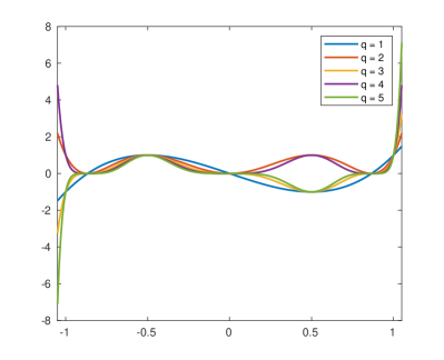
(b) Power of Chebyshev polynomial $T_{3}^{q}(t)$

In order to suppress all eigenvalues in a general interval $[a,b]$, a linear mapping from $[a,b]$ to $[-1,1]$ is constructed. To be precise, the polynomial can be chosen as

(2.2) $$\rho(t)=T_{d}\left(\frac{t-(b+a)/2}{(b-a)/2}\right).$$

After the polynomial filters are applied, an orthogonalization step usually follows in order to prevent the subspace from losing rank. This step is often performed by a single QR decomposition. Consequently, given an arbitrary matrix $U\in\mathbb{R}^{n\times p}$ and a polynomial $\rho(t)$, the polynomial-filtered subspace iteration can be simply written as

(2.3) $$U^{+}=\mathrm{orth}(\rho(A)U),$$

where “$\mathrm{orth}$” stands for the orthogonalization operation. In most cases, the updated matrix $U^{+}$ spans a subspace which contains some approximated eigenvectors of $A$. By extracting eigen-pairs from this subspace, we are able to derive a number of polynomial-filtered inexact optimization methods. In the next subsections we present two examples: PFPG and PFAM.

2.2 The PFPG Method

In this subsection we show how to apply the subspace update (2.3) to the proximal gradient method, on a set of problems with a general form. Consider the following unconstrained spectral operator minimization problem

(2.4) $$\begin{array}[]{rl}\min&h(x):=F(x)+R(x),\\ \end{array}$$

where $F(x)$ has a composition form $F(x)=f\circ\lambda(\mathcal{B}(x))$ with $\mathcal{B}(x)=G+\mathcal{A}^{*}(x)$ and $R(x)$ is a regularizer with simple structures but need not be smooth. Here $G$ is a known matrix in $\mathcal{S}^{n}$, and $\mathcal{A}^{*}:\mathbb{R}^{m}\rightarrow\mathcal{S}^{n}$ is a linear operator. The function $f:\mathbb{R}^{n}\rightarrow\mathbb{R}$ is smooth and absolutely symmetric, i.e., $f(x)=f(Px)$ for all $x\in\mathbb{R}^{n}$ and any permutation matrix $P\in\mathbb{R}^{n\times n}$. It can be easily verified that $F(x)$ is well defined.

According to [16, Section 6.7.2], the gradient of $F$ in (2.4) is

(2.5) $$\nabla F(x)=\mathcal{A}(\Psi(\mathcal{B}(x))),$$

where $\Psi$ is a spectral operator defined by

$$\Psi(X)=V\mathrm{Diag}(\nabla f(\lambda(X)))V^{T},$$

and $V\mathrm{Diag}(\lambda(X))V^{T}$ is the full eigen-decomposition of $X$.

For any matrix $S\in\mathbb{R}^{n\times p}$, let $\mathcal{P}_{S}$ denote the projection operator on subspace $\mathrm{Range}(S)$. When $S$ is an orthogonal matrix, the operator $\mathcal{P}_{S}$ is defined by

(2.6) $$\mathcal{P}_{S}(X)=SS^{T}XSS^{T}.$$

If $V$ is exactly a $p$-dimensional eigen-space of the matrix $X$, the eigenvalue decomposition of $\mathcal{P}_{V}(X)$ can be written as

(2.7) $$\mathcal{P}_{V}(X)=\begin{bmatrix}\tilde{V}&V_{\perp}\end{bmatrix}\begin{bmatrix}\Lambda_{p}&O\\ O&O\end{bmatrix}\begin{bmatrix}\tilde{V}^{T}\\ V_{\perp}^{T}\end{bmatrix},$$

where $(\tilde{V},\Lambda_{p})$ is the corresponding eigen-pairs and we have $\mathrm{Range}(V)=\mathrm{Range}(\tilde{V})$. Note that $(\tilde{V},\Lambda_{p})$ has closed-form expression with $\tilde{V}=VY$ where $Y\Lambda_{p}Y^{T}$ is the full eigenvalue decomposition of $H:=V^{T}XV\in\mathbb{R}^{p\times p}$.

Suppose evaluating $\nabla F$ only involves a small number of eigenvalues in the problem (2.4), then we are able to compute $\nabla F$ quickly as long as the corresponding subspace is given. We summarize them in Assumption 1.

Assumption 1.

1. Let $\mathcal{I}(x)\subset[n]$ be an integer set with $\mathcal{I}(x)=\{s,s+1,...,t\}$ and suppose that the gradient of $F(x)$ in (2.4) has the relationship

   (2.8) $$\nabla F(x)=\bar{g}:=\mathcal{A}(\Phi(\mathcal{P}_{V_{\mathcal{I}}}(\mathcal{B}(x)))),$$

   where $\Phi$ is a spectral operator and $V_{\mathcal{I}}\in\mathbb{R}^{n\times|\mathcal{I}|}$ contains eigenvectors $v_{i},i\in\mathcal{I}(x)$ of $\mathcal{B}(x)$.

2. $\Phi$ is Lipschitz continuous with a factor $L_{\Phi}$,

   (2.9) $$\|\Phi(X)-\Phi(Y)\|_{F}\leq L_{\Phi}\|X-Y\|_{F}.$$

We now compare the gradient expression (2.8) in Assumption 1 with the original gradient (2.5). Expression (2.8) implies that the subspace $V_{\mathcal{I}}$ contains all information for evaluating $\nabla F(x)$. In other words, we do not need full eigenvalue decompositions as indicated by (2.5). The spectral operator $\Phi(\cdot)$ in (2.8) is also different from $\Psi(\cdot)$ defined in (2.5). The choice of $\Phi(\cdot)$ can be arbitrary as long as it satisfies Assumption 1. In most cases $\Phi(\cdot)$ inherits the definition of $\Psi(\cdot)$ but they need not be the same. Under the Assumption 1, we can write the proximal gradient algorithm as

(2.10) $$x^{k+1}=\mathrm{prox}_{\tau_{k}R}(x^{k}-\tau_{k}\mathcal{A}(\Phi(\mathcal{P}_{V^{k}_{\mathcal{I}_{k}}}(\mathcal{B}(x^{k}))),$$

where $V^{k}_{\mathcal{I}_{k}}$ contains the eigenvectors of $\mathcal{B}(x^{k})$ at iteration $k$, $\tau_{k}$ is the step size, and the proximal operator is defined by

(2.11) $$\mathrm{prox}_{tR}(x)=\operatornamewithlimits{argmin}_{u}R(u)+\frac{1}{2t}\|u-x\|_{2}^{2}.$$

In the scheme (2.10), the main cost is the computation of the EVD of $\mathcal{P}_{V^{k}_{\mathcal{I}_{k}}}(\mathcal{B}(x^{k}))$ as the exact subspace $V^{k}_{\mathcal{I}_{k}}$ is unknown. Thus, an idea to reduce the expenses is to use polynomial filters to generate an approximation of eigen-space. Then it is easy to compute the projection on this space and the corresponding eigen-decomposition, whence the image of the spectral operator on the projection matrix, as shown in (2.7). To obtain a good approximation, the update of eigen-space is by means of Chebyshev polynomials which can suppress all unwanted eigenvectors of $\mathcal{B}(x)$ and the eigen-space in last step is used as initial values. In summary, the proximal gradient method with polynomial filters can be written as

(2.12) $$x^{k+1} = \mathrm{prox}_{\tau_{k}R}(x^{k}-\tau_{k}\mathcal{A}(\Phi(\mathcal{P}_{U^{k}}(\mathcal{B}(x^{k})))),$$

(2.13) $$U^{k+1} = \mathrm{orth}(\rho_{k+1}^{q_{k+1}}(\mathcal{B}(x^{k+1}))U^{k}),$$

where $U^{k}\in\mathbb{R}^{n\times p}$ with $p\geq|\mathcal{I}_{k}|$ is an orthogonal matrix which serves as an approximation of $V^{k}_{\mathcal{I}_{k}}$ each step, and $q_{k}\geq 1$ is a small integer (usually 1 to 3) which means the polynomial is applied for $q_{k}$ times before the orthogonalization.

We mention that (2.12) and (2.13) are actually two different updates that couple together. Given a subspace spanned by $U^{k}$, the step (2.12) performs the proximal gradient descent with the approximated gradient extracted from $U^{k}$. The next step (2.13) makes refinement on the subspace to obtain $U^{k+1}$ via polynomial filters. The subspace will become more and more exact as the iterations proceed. In practice, it is usually observed that $U^{k}$ is very “close” to the true eigen-space $V^{k}_{\mathcal{I}_{k}}$ during the last iterations of the algorithm.

2.3 The PFAM Method

Consider the following standard SDP:

(2.14) $$\begin{array}[]{rl}\min&\langle C,X\rangle,\\ \mbox{ s.t. }&\mathcal{A}X=b,X\succeq 0,\end{array}$$

where $\mathcal{A}$ is a bounded linear operator. Let $F(X)=1_{\{X\succeq 0\}}(X)$ and $G(X)=1_{\{\mathcal{A}X=b\}}(X)+\langle C,X\rangle$, where $1_{\Omega}(X)$ is the indicator function on a set $\Omega$. Then the Douglas-Rachford Splitting (DRS) method on the primal SDP (2.14) can be written as

$$Z^{k+1}=T_{\textrm{DRS}}(Z^{k}),$$

where

$$T_{\textrm{DRS}}=\mathrm{prox}_{tG}(2\mathrm{prox}_{tF}-I)-\mathrm{prox}_{tF}+I,$$

which is equivalent to the ADMM on the dual problem. The explicit forms of $\mathrm{prox}_{tF}(Z)$ and $\mathrm{prox}_{tG}(Y)$ can be written as

$$\mathrm{prox}_{tF}(Z) = \mathcal{P}_{+}(Z),$$

$$\mathrm{prox}_{tG}(Y) = (Y+tC)-\mathcal{A}^{*}(\mathcal{A}\mathcal{A}^{*})^{-1}(\mathcal{A}Y+t\mathcal{A}C-b),$$

where $\mathcal{P}_{+}(Z)$ is the projection operator onto the positive semi-definite cone.

Similar to the PFPG method, $\mathcal{P}_{+}(Z)$ is only determined by the eigen-space spanned by the positive eigenvectors of $Z$, so we are able to use the polynomial filters to extract an approximation $U^{k}$. Therefore, the PFAM can be written as

(2.15) $$Z^{k+1} = \mathrm{prox}_{tG}(2\mathcal{P}_{+}(\mathcal{P}_{U^{k}}(Z^{k}))-Z^{k})-\mathcal{P}_{+}(\mathcal{P}_{U^{k}}(Z^{k}))+Z^{k},$$

(2.16) $$U^{k+1} = \mathrm{orth}(\rho_{k+1}^{q_{k+1}}(Z^{k+1})U^{k}),$$

where $U^{k}\in\mathbb{R}^{n\times p}$ with $p\geq|\mathcal{I}|$ is an orthogonal matrix and $q_{k}\geq 1$ is a small integer.

3 Convergence Analysis

3.1 Preliminary

In this section we introduce some basic notations and tools that are used in our analysis. Firstly, we introduce the definition of principal angles to measure the distance between two subspaces.

Definition 3.1.

Let $X,Y\in\mathbb{R}^{n\times p}$ be two orthogonal matrices. The singular values of $X^{T}Y$ are $\sigma_{1}\geq\sigma_{2}\geq\cdots\geq\sigma_{p}$, which lie in $[0,1]$. The principal angle between $\mathrm{Range}(X)$ and $\mathrm{Range}(Y)$ is defined by

(3.1) $$\Theta(X,Y):=\mathrm{Diag}(\arccos\sigma_{1},\ldots,\arccos\sigma_{p}),$$

In particular, we define $\sin\Theta$ by taking the sine of $\Theta$ componentwisely.

The following lemma describes a very important property of Chebyshev polynomials.

Lemma 3.2.

The Chebyshev polynomials increase fast outside $[-1,1]$, i.e.,

(3.2) $$T_{d}(\pm(1+\epsilon))\geq 2^{d\min\{\sqrt{\epsilon},1\}-1},\ \forall\epsilon>0.$$

Proof 3.3.

It follows from the expression (2.1) that

$$T_{d}(\pm(1+\epsilon)) \geq \frac{1}{2}(1+\epsilon+\sqrt{2\epsilon+\epsilon^{2}})^{d}\geq\frac{1}{2}(1+\sqrt{\epsilon})^{d}$$

$$= \frac{1}{2}e^{d\log(1+\sqrt{\epsilon})}\geq 2^{d\min\{\sqrt{\epsilon},1\}-1},$$

where the last inequality follows from that $\log(1+x)\geq\log 2\cdot\min\{x,1\}$.

3.2 Convergence analysis for PFPG

In this subsection, we analyze the convergence for general convex problems. The relative gap is defined by

(3.3) $$\mathcal{G}_{k}=\min_{i\in\mathcal{I}_{k}}\left(\frac{|\lambda_{i}-(a_{k}+b_{k})/2|}{(a_{k}-b_{k})/2}-1\right),$$

where $[a_{k},b_{k}]$ is the interval suppressed by Chebyshev polynomials at the $k$-th iteration, $\mathcal{I}_{k}$ is the index set of the eigenvalues beyond $[a_{k},b_{k}]$. Throughout this section, we make the following assumptions.

Assumption 2.

1. $\|\sin\Theta(V^{k+1}_{\mathcal{I}_{k+1}},U^{k})\|_{2}<\gamma,\ \forall\ k$ with $\gamma<1$, where $V^{k}_{\mathcal{I}_{k}}$ and $U^{k}$ are defined in Assumption 1 and (2.13) at iteration $k$.

2. The sequence generated by iteration (2.12) and (2.13) are bounded, i.e., $\|x^{k}\|_{2}\leq C,\ \forall\ k.$

3. The relative gap (3.3) has a lower bound, i.e., $\mathcal{G}_{k}\geq l,\ \forall\ k$.

Assumption (i) implies that the initial eigen-space is not orthogonal to the truely wanted eigen-space so that we can obtain $V^{k+1}_{\mathcal{I}_{k+1}}$ by performing subspace iterations on $U^{k}$. Essentially, this property is required by almost all iterative eigensolvers for finding the correct eigenspace at each iteration. Assumption (ii) is commonly used in the optimization literature. Assumption (iii) is a key assumption which guarantees that the relative gap $\mathcal{G}_{k}$ exists in the asymptotic sense. Therefore, the polynomial filters are able to separate the wanted eigenvalues from the unwanted ones. In eigenvalue computation, this property is often enforced by adding a sufficient number of guarding vectors so that the corresponding eigenvalue gap is large enough.

The following lemma gives an error estimation when using an inexact gradient of $F$. It states that the polynomial degree $d_{k}$ should be proportional to $\log(1/\varepsilon)$, where $\varepsilon$ is a given tolerance.

Lemma 3.4.

Suppose that Assumptions 1 and 2 hold. Define the error between the exact and inexact gradients:

(3.4) $$e^{k}=\mathcal{A}(\Phi(\mathcal{P}_{U^{k}}(\mathcal{B}(x^{k}))))-\nabla F(x^{k}).$$

Let the polynomial filter $\rho_{k}(t)$ be a Chebyshev polynomial with degree $d_{k}$. To achieve $\|e^{k}\|_{2}\leq\varepsilon$ for a given tolerance $0<\varepsilon<1$, the degree $d_{k}$ should satisfy

(3.5) $$d_{k}=\Omega\left(\frac{\log\frac{1}{\varepsilon}}{\min\{l,1\}}\right).$$

Proof 3.5.

The update (2.1) can be regarded as one orthogonal iteration. The eigenvalue of $\rho_{k}^{q_{k}}(\mathcal{B}(x^{k}))$ is $\rho_{k}^{q_{k}}(\lambda_{i})$, where $\lambda_{i}$’s are the eigenvalues of $\mathcal{B}(x^{k})$. According to Lemma 3.2, the eigenvalues have the following distribution after we apply the Chebyshev polynomial:

$$\min_{i\in\mathcal{I}_{k}}\rho_{k}^{q_{k}}(\lambda_{i})\geq 2^{q_{k}d_{k}\min\{\sqrt{l},1\}-q_{k}}\text{ and }\max_{i\notin\mathcal{I}_{k}}\rho_{k}^{q_{k}}(\lambda_{i})\leq 1.$$

It follows from [9, Theorem 8.2.2] that

(3.6) $$\|\sin\Theta(V_{\mathcal{I}_{k}}^{k},U^{k})\|_{2}\leq\frac{2^{q_{k}}}{2^{q_{k}d_{k}\min\{l,1\}}}\frac{\gamma}{\sqrt{1-\gamma^{2}}}.$$

Due to the boundness of $\mathcal{A}$ and the Lipschitz continuity of $\Phi$, we have

(3.7) $$\|e^{k}\|_{2}\leq c_{1}\|\mathcal{P}_{U^{k}}(\mathcal{B}(x^{k}))-\mathcal{P}_{V_{\mathcal{I}_{k}}^{k}}(\mathcal{B}(x^{k}))\|_{F},$$

where $c_{1}$ is a constant. It is shown in [9, Theorem 2.5.1] that $\|\sin\Theta(X,Y)\|_{2}=\|XX^{T}-YY^{T}\|_{2}.$ Using this identity, we have

(3.8) $$\begin{split}&\|\mathcal{P}_{U^{k}}(\mathcal{B}(x^{k}))-\mathcal{P}_{V_{\mathcal{I}_{k}}^{k}}(\mathcal{B}(x^{k}))\|_{F}\\ \leq&\|\mathcal{P}_{U^{k}}(\mathcal{B}(x^{k}))-U^{k}(U^{k})^{T}(\mathcal{B}(x^{k}))V_{\mathcal{I}_{k}}^{k}(V_{\mathcal{I}_{k}}^{k})^{T}\|_{F}+\|U^{k}(U^{k})^{T}(\mathcal{B}(x^{k}))V_{\mathcal{I}_{k}}^{k}(V_{\mathcal{I}_{k}}^{k})^{T}-\mathcal{P}_{V_{\mathcal{I}_{k}}^{k}}(\mathcal{B}(x^{k}))\|_{F}\\ \leq&2||\mathcal{B}(x^{k})||_{F}\|\sin\Theta(V_{\mathcal{I}_{k}}^{k},U^{k})\|_{2}\\ \leq&\frac{c_{2}\cdot 2^{q_{k}}}{2^{q_{k}d_{k}\min\{l,1\}}},\end{split}$$

where $c_{2}$ is a constant depending on $\gamma$. The second inequality is due to the fact that $\|AB\|_{F}\leq\|A\|_{2}\|B\|_{F}$ and the last inequality follows from (3.6) and the boundedness of $\mathcal{A}$ and $x^{k}$. It is easy to verify that $\|e^{k}\|\leq\varepsilon$ if (3.5) holds for any $\varepsilon\in(0,1)$. This completes the proof.

We claim that $\nabla F(x)$ is Lipschitz continuous due to the boundness of $\mathcal{A}$ and $x^{k}$ and the Lipschitz continuity of $\Phi$. In the following part, we define the Lipschitz constant of $\nabla F(x)$ by $L$. The following theorem gives the convergence of the PFPG method.

Theorem 3.6.

Suppose that Assumptions 1 and 2 hold. Let $\tau_{k}=\tau\leq\frac{1}{L}$ and $\bar{x}_{K}=\frac{1}{K}\sum_{k=1}^{K}x^{k}$. Then the convergence $\lim_{K\rightarrow\infty}h(\bar{x}^{K})=h(x^{*})$ holds if

(3.9) $$d_{k}=\Omega\left(\frac{\log k}{\min\{l,1\}}\right).$$

Proof 3.7.

For simplicity we define the noisy residual function by

$$r_{\tau}(x,e)=\frac{1}{\tau}(x-\mathrm{prox}_{\tau R}(x-\tau(\nabla F(x)+e))).$$

Then the update (2.12) can be written as

$$x^{k}-x^{k+1}=\tau_{k}r_{\tau_{k}}(x^{k},e^{k}).$$

According to the Lipschitz continuity of $\nabla F$, we have

$$h(x^{k+1})\leq F(x^{k})-\tau_{k}\nabla F(x^{k})^{T}(r_{\tau_{k}}(x^{k},e^{k}))+\frac{L\tau_{k}^{2}}{2}\|r_{\tau_{k}}(x^{k},e^{k})\|_{2}^{2}+R(x^{k+1}).\\$$

By the convexity of $F(x)$ and $R(x)$ and $r_{\tau_{k}}(x,e^{k})-\nabla F(x^{k})-e^{k}\in\partial R(x^{k+1})$, we have

$$h(x^{k+1}) \leq F(x^{*})+\nabla F(x^{k})^{T}(x^{k}-x^{*})-\tau_{k}\nabla F(x^{k})^{T}(r_{\tau_{k}}(x^{k},e^{k}))+\frac{L\tau_{k}^{2}}{2}\|r_{\tau_{k}}(x^{k},e^{k})\|_{2}^{2}$$

$$+R(x^{*})+(r_{\tau_{k}}(x^{k},e^{k})-\nabla F(x^{k})-e^{k})^{T}(x^{k+1}-x^{*}).$$

Setting the step size $\tau_{k}=\tau\leq\frac{1}{L}$ yields

$$h(x^{k+1})-h(x^{*}) \leq \nabla F(x^{k})^{T}(x^{k}-x^{*})-\tau\nabla F(x^{k})^{T}(r_{\tau}(x^{k},e^{k}))+\frac{\tau}{2}\|r_{\tau}(x^{k},e^{k})\|_{2}^{2}$$

$$+(r_{\tau}(x^{k},e^{k})-\nabla F(x^{k})-e^{k})^{T}(x^{k+1}-x^{*}).$$

After rearranging and applying the boundness of the sequence $x^{k}$, we have

$$h(x^{k+1})-h(x^{*}) \leq \frac{1}{2\tau}(\|x^{k}-x^{*}\|_{2}^{2}-\|x^{k+1}-x^{*}\|_{2}^{2})+(C+\|x^{*}\|)\|e^{k}\|_{2},$$

where $C$ is a constant. Then it follows that

(3.10) $$h(\bar{x}^{K})-h(x^{*})\leq\frac{1}{K}\sum_{k=1}^{K}(h(x^{k})-h(x^{*}))\leq\frac{1}{2K\tau}\|x^{0}-x^{*}\|_{2}^{2}+\frac{C+\|x^{*}\|}{K}\sum_{k=1}^{K}\|e^{k}\|_{2}.$$

According to Lemma 3.4, by setting $d_{k}=\Omega\left(\frac{\log k}{\min\{l,1\}}\right)$ at iteration $k$, we have the upper bound $\sum_{k=1}^{K}\|e^{k}\|_{2}\leq\sum_{k=1}^{K}1/k$. Thus the right hand side of (3.10) goes to zero as $K\rightarrow\infty$, which completes the proof.

The following theorem gives a linear convergence rate under the strongly convex assumption of $F(x)$.

Theorem 3.8.

Suppose that Assumptions 1 and 2 hold, and $F(x)$ is $\mu$-strongly convex. Let $\tau_{k}=\tau\leq\frac{1}{L}$ and $w\leq\frac{\mu}{2}$. Then a linear convergence rate is achieved if

(3.11) $$d_{k}=\Omega\left(\frac{-\log(w\|x^{k+1}-x^{*}\|_{2})}{\min\{l,1\}}\right).$$

Proof 3.9.

The quadratic bound in the proof of Theorem 3.6 gives

$$h(x^{k+1})\leq F(x^{k})-\tau_{k}\nabla F(x^{k})^{T}(r_{\tau_{k}}(x^{k},e^{k}))+\frac{L\tau_{k}^{2}}{2}\|r_{\tau_{k}}(x^{k},e^{k})\|_{2}^{2}+R(x^{k+1}).\\$$

By the stongly convexity of $F(x)$, the convexity of $R(x)$ and $r_{\tau_{k}}(x^{k},e^{k})-\nabla F(x^{k})-e^{k}\in\partial R(x^{k+1})$, we have

$$h(x^{k+1}) \leq F(x^{*})+\nabla F(x^{k})^{T}(x^{k}-x^{*})-\frac{\mu}{2}\|x^{k}-x^{*}\|_{2}^{2}-\tau_{k}\nabla F(x^{k})^{T}(r_{\tau_{k}}(x^{k},e^{k}))$$

$$+\frac{L\tau_{k}^{2}}{2}\|r_{\tau_{k}}(x^{k},e^{k})\|_{2}^{2}+R(x^{*})+(r_{\tau_{k}}(x^{k},e^{k})-\nabla F(x^{k})-e^{k})^{T}(x^{k+1}-x^{*}).$$

Under the choice of step size $\tau_{k}=\tau\leq\frac{1}{L}$, we have

$$h(x^{k+1})-h(x^{*}) \leq \nabla F(x^{k})^{T}(x^{k}-x^{*})-\tau\nabla F(x^{k})^{T}(r_{\tau}(x^{k},e^{k}))+\frac{\tau}{2}\|r_{\tau}(x^{k},e^{k})\|_{2}^{2}$$

$$-\frac{\mu}{2}\|x^{k}-x^{*}\|_{2}^{2}+(r_{\tau}(x^{k},e^{k})-\nabla F(x^{k})-e^{k})^{T}(x^{k+1}-x^{*})$$

$$= \frac{1}{2\tau}((1-\mu\tau)\|x^{k}-x^{*}\|_{2}^{2}-\|x^{k+1}-x^{*}\|_{2}^{2})-(e^{k})^{T}(x^{k+1}-x^{*})$$

$$\leq \frac{1}{2\tau}((1-\mu\tau)\|x^{k}-x^{*}\|_{2}^{2}-\|x^{k+1}-x^{*}\|_{2}^{2})+\|e^{k}\|_{2}\|x^{k+1}-x^{*}\|_{2}.$$

Together with $h(x^{k+1})\geq h(x^{*})$, we have

(3.12) $$\|x^{k+1}-x^{*}\|_{2}^{2}\leq(1-\mu\tau)\|x^{k}-x^{*}\|_{2}^{2}+2\tau\|e^{k}\|_{2}\|x^{k+1}-x^{*}\|_{2}.$$

The choice of $d_{k}$ guarantees $\|e^{k}\|_{2}\leq w\|x^{k+1}-x^{*}\|_{2}.$ Plugging this upper bound of $\|e^{k}\|$ into (3.12) yields

$$\|x^{k+1}-x^{*}\|^{2}_{2}\leq\eta\|x^{k}-x^{*}\|_{2}^{2},$$

where $\eta=\frac{1-\mu\tau}{1-2w\tau}<1$, which completes the proof.

3.3 Warm-start analysis for PFPG

In this section, we analyze the linear convergence of PFPG under the warm-start setting. Suppose that $\rho_{k}(\lambda_{s_{i}}(\mathcal{B}(x^{k}))$ are in decreasing order, and define

(3.13) $$\eta_{k}=\frac{\rho_{k}(\lambda_{s_{p+1}}(\mathcal{B}(x^{k}))}{\rho_{k}(\lambda_{s_{p}}(\mathcal{B}(x^{k}))}.$$

We should point out that under Assumption 3, $\eta_{k}$ is strictly smaller than 1 since $\mathcal{G}_{k}\geq l>0$. An additional assumption is needed if we intend to refine the subspace from the previous one.

Assumption 3.

$\|\sin\Theta(V^{k+1}_{\mathcal{I}_{k+1}},V^{k}_{\mathcal{I}_{k}})\|_{2}\leq c_{1}\|x^{k+1}-x^{k}\|_{2}$ for all $k$.

Assumption 3 means that the eigen-space at two consecutive iteration points are close enough. This is necessary since we use the eigen-space at the previous step as the initial value of polynomial filter. This assumption is satisfied when the gap is large enough by the Davis-Kahan $\sin\Theta$ theorem [5].

The next lemma shows the relationship between the two iterations in a recursive form. It plays a key role in the proof of the main convergence theorem.

Lemma 3.10.

Suppose that Assumptions 1, 2 and 3 hold. Let $\mathcal{X}$ be the set of optimal solutions of the problem (2.4), and $\mathrm{dist}(x,\mathcal{X})=\inf_{y\in\mathcal{X}}\|x-y\|_{2}$ be the distance between $x$ and $\mathcal{X}$. Then we have

(3.14) $$\|\sin\Theta(V^{k+1}_{\mathcal{I}_{k+1}},U^{k+1})\|_{2}\leq\eta_{k+1}^{q_{k}}(c_{2}\|\sin\Theta(V^{k}_{\mathcal{I}_{k}},U^{k})\|_{2}+c_{3}\mathrm{dist}(x^{k},\mathcal{X})),$$

where $c_{2}$ and $c_{3}$ are constants.

Proof 3.11.

The update (2.3) can be seen as one iteration in the orthogonal iteration. Then it follows from [9, Theorem 8.2.2] that

$$\|\sin\Theta(V^{k+1}_{\mathcal{I}_{k+1}},U^{k+1})\|_{2}\leq\eta_{k+1}^{q_{k}}\|\tan\Theta(V^{k+1}_{\mathcal{I}_{k+1}},U^{k})\|_{2}\leq\frac{\eta_{k+1}^{q_{k}}}{\sqrt{1-\gamma^{2}}}\|\sin\Theta(V^{k+1}_{\mathcal{I}_{k+1}},U^{k})\|_{2},$$

According to (3.7) and (3.8) in Lemma 3.4, we have

$$\|e^{k}\|_{2}\leq c_{4}\|\sin\Theta(V^{k}_{\mathcal{I}_{k}},U^{k})\|_{2},$$

where $c_{4}$ is a constant. The upper bound of $\|x^{k}-x^{k+1}\|_{2}$ is given by

$$\|x^{k}-x^{k+1}\|_{2}\leq\tau_{k}(\|r_{\tau_{k}}(x^{k},e^{k})-r_{\tau_{k}}(x^{k},0)\|_{2}+\|r_{\tau_{k}}(x^{k},0)\|_{2})$$

$$\leq \tau_{k}\|e^{k}\|_{2}+\omega\mathrm{dist}(x^{k},\mathcal{X})$$

$$\leq \tau_{k}c_{4}\|\sin\Theta(V_{\mathcal{I}_{k}}^{k},U^{k})\|_{2}+\omega\mathrm{dist}(x^{k},\mathcal{X}),$$

where the second inequality is due to the monotonity of the proximal operator and the cocoercivity with modulus $\omega$ of the residual function $r_{\tau_{k}}(x^{k},0)$. Finally, we obtain

$$\|\sin\Theta(V^{k+1}_{\mathcal{I}_{k+1}},U^{k+1})\|_{2}\leq\frac{\eta_{k+1}^{q_{k}}}{\sqrt{1-\gamma^{2}}}\|\sin\Theta(V^{k+1}_{\mathcal{I}_{k+1}},U^{k})\|_{2}$$

$$\leq \frac{\eta_{k+1}^{q_{k}}}{\sqrt{1-\gamma^{2}}}(\|\sin\Theta(V^{k}_{\mathcal{I}_{k}},U^{k})\|_{2}+\|\sin\Theta(V^{k+1}_{\mathcal{I}_{k+1}},V^{k}_{\mathcal{I}_{k}}\|_{2})$$

$$\leq \frac{\eta_{k+1}^{q_{k}}}{\sqrt{1-\gamma^{2}}}(\|\sin\Theta(V^{k}_{\mathcal{I}_{k}},U^{k})\|_{2}+c_{1}\|x^{k}-x^{k+1}\|_{2})$$

$$\leq \frac{\eta_{k+1}^{q_{k}}}{\sqrt{1-\gamma^{2}}}((1+\tau_{k}c_{1}c_{4})\|\sin\Theta(V^{k}_{\mathcal{I}_{k}},U^{k})\|_{2}+c_{1}\omega\mathrm{dist}(x^{k},\mathcal{X})),$$

where the third inequality is from (iii) in Assumption 3. This completes the proof.

Lemma 3.10 means that the principle angle between $V^{k+1}_{\mathcal{I}_{k+1}}$ and $U^{k+1}$ are determined by the angle in the previous iteration and how far $x^{k}$ is from the optimal set $\mathcal{X}$. As an intuitive interpretation, the polynomial-filtered subspace becomes more and more accurate when PFPG is close to converge.

We are now ready to state the main result. It implies that the PFPG method has a linear convergence rate if the polynomial degree is a constant, independent of the iteration $k$.

Theorem 3.12.

Suppose that Assumptions 1, 2 and 3 holds, and the exact proximal gradient method for (2.4) has a linear convergence rate, i.e.,

(3.15) $$\mathrm{dist}(\mathrm{prox}_{\tau R}(x^{k}-\tau_{k}\nabla F(x^{k})),\mathcal{X})\leq\nu\mathrm{dist}(x^{k},\mathcal{X}),\nu\in(0,1).$$

If $\eta_{k+1}$ (3.13) satisfies

(3.16) $$\frac{\nu+\eta_{k+1}^{q_{k}}c_{3}}{2}+\sqrt{\left(\frac{\nu+\eta_{k+1}^{q_{k}}c_{3}}{2}\right)^{2}+\eta_{k+1}^{q_{k}}(\tau_{k}c_{2}c_{4}-\nu c_{3})}<\rho<1,$$

where $c_{2},c_{3},c_{4}$ are constants in Lemma 3.10, then the PFPG method has a linear convergence rate.

Proof 3.13.

Since $\mathcal{X}$ is closed, we denote $x_{prj}$ as the projection of $\mathrm{prox}_{\tau_{k}R}(x^{k}-\tau_{k}\nabla F(x^{k}))$ onto the optimal set $\mathcal{X}$. Then we have

(3.17) $$\begin{split}&\mathrm{dist}(x^{k+1},\mathcal{X})\leq\|\mathrm{prox}_{\tau_{k}R}(x^{k}-\tau_{k}(\nabla F(x^{k})+e^{k}))-x_{prj}\|_{2}\\ \leq&\|\mathrm{prox}_{\tau_{k}R}(x^{k}-\tau_{k}\nabla F(x^{k}))-\mathrm{prox}_{\tau_{k}R}(x^{k}-\tau_{k}(\nabla F(x^{k})+e^{k}))\|_{2}\\ &+\|\mathrm{prox}_{\tau_{k}R}(x^{k}-\tau_{k}\nabla F(x^{k}))-x_{prj}\|_{2}\\ \leq&\mathrm{dist}(\mathrm{prox}_{\tau_{k}R}(x^{k}-\tau_{k}\nabla F(x^{k})),\mathcal{X})+\tau_{k}\|e^{k}\|_{2}\\ \leq&\mathrm{dist}(\mathrm{prox}_{\tau_{k}R}(x^{k}-\tau_{k}\nabla F(x^{k})),\mathcal{X})+\tau_{k}c_{4}\|\sin\Theta(V^{k}_{\mathcal{I}_{k}},U^{k})\|_{F}\\ \leq&\nu\mathrm{dist}(x^{k},\mathcal{X})+\tau_{k}c_{4}\|\sin\Theta(V_{\mathcal{I}_{k}}^{k},U^{k})\|_{F},\ \end{split}$$

where the first inequality is from the definition of the distance function, the second inequality is from the triangle inequality, the third inequality is shown in the proof of Lemma 3.10 and the last inequality is due to the linear convergence of the proximal gradient method.

From (3.14) and (LABEL:eqn:recr2) we observe that the error $\mathrm{dist}(x^{k},\mathcal{X})$ and $\|\sin\Theta(V_{\mathcal{I}_{k}}^{k},U^{k})\|_{2}$ are coupled together. Thus we define the error vector

(3.18) $$s^{k}=\left[\begin{matrix}\mathrm{dist}(x^{k},\mathcal{X})\\ \|\sin\Theta(V_{\mathcal{I}_{k}}^{k},U^{k})\|_{2}\end{matrix}\right].$$

The two recursive formula can be rewritten as

(3.19) $$s^{k+1}\leq R^{k}s^{k},\ R^{k}=\left[\begin{matrix}\nu&\tau_{k}c_{4}\\ \eta_{k+1}^{q_{k}}c_{2}&\eta_{k+1}^{q_{k}}c_{3}\\ \end{matrix}\right].$$

The spectral radius of $R^{k}$ is bounded by the left term in (3.16). It is easy to verify that (3.16) holds if the degree $d_{k}$ is large enough to make $\eta_{k+1}$ sufficiently small. The choice of $d_{k}$ is independent of the iteration number $k$. This completes the proof.

Theorem 3.12 requires the linear convergence rate of the exact proximal gradient method. This condition is satisfied if $F(x)$ is strongly convex and smooth. From the proof we also observe that $\mathrm{dist}(x^{k},\mathcal{X})$ and $\|\sin\Theta(V_{\mathcal{I}_{k}}^{k},U^{k})\|_{2}$ are recursively bounded by each other. By choosing suitable $d_{k}$, the two errors are able to decay simultaneously.

3.4 Convergence analysis for PFAM

We next analyze the convergence of PFAM. Similar to PFPG, we make the following assumptions:

Assumption 4.

Let $V_{\mathcal{I}_{k}}^{k}$ be an orthogonal matrix whose columns are the eigenvectors corresponding to all positive eigenvalues of $Z^{k}$.

1. $\|\sin\Theta(V^{k+1}_{\mathcal{I}_{k+1}},U^{k})\|_{2}<\gamma,\ \forall\ k$ with $\gamma<1$.

2. The sequence generated by (2.15) and (2.16) is bounded, i.e., $\|Z^{k}\|_{F}\leq C,\ \forall\ k.$

3. The relative gap (3.3) has a lower bound, i.e., $\mathcal{G}_{k}\geq l,\ \forall\ k$.

The main theorem is established by following the proof in [6].

Theorem 3.14.

Suppose Assumption 4 holds. The convergence $\|Z^{k}-T_{\textrm{DRS}}(Z^{k})\|_{F}=\mathcal{O}(1/\sqrt{k})$ is archived if

(3.20) $$d_{k}=\Omega\left(\frac{\log k}{\min\{l,1\}}\right).$$

Proof 3.15.

According to the proof of Lemma 3.4, we obtain

$$\|\mathcal{P}_{U^{k}}(Z^{k})-\mathcal{P}_{V_{\mathcal{I}_{k}}^{k}}(Z^{k})\|_{F}\leq\frac{c\cdot 2^{q_{k}}}{2^{q_{k}d_{k}\min\{l,1\}}},$$

where $c$ is a constant. Define the error between one PFAM update and one DRS iteration $E^{k}=Z^{k+1}-T_{\textrm{DRS}}(Z^{k})$. Since $\mathrm{prox}_{tG}$ and $\mathcal{P}_{+}$ are Lipschitz continuous with constant $L_{1}$ and $L_{2}$, we have

$$\|E^{k}\|_{F}\leq(2L_{1}L_{2}+L_{2})\|\mathcal{P}_{U^{k}}(Z^{k})-\mathcal{P}_{V_{\mathcal{I}_{k}}^{k}}(Z^{k})\|_{F}\leq\frac{c_{2}\cdot 2^{q_{k}}}{2^{q_{k}d_{k}\min\{l,1\}}},$$

where $c_{2}$ is a constant. Let $s>1$ be an arbitrary number, the error can be controlled with an order

$$\|E^{k}\|_{F}=\mathcal{O}(\frac{1}{k^{s}}),$$

by choosing $d_{k}=\Omega(\frac{s\log l}{\min(l,1)})$.

Define $W^{k}=T_{\textrm{DRS}}(Z^{k})-Z^{k}$, $S^{k}=Z^{k+1}-Z^{k}$ and $T^{k}=T_{\textrm{DRS}}(Z^{k+1})-T_{\textrm{DRS}}(Z^{k})$. Then we have

(3.21) $$\begin{split}\|W^{k+1}\|_{F}^{2}&=\|W^{k}\|_{F}^{2}+\|W^{k+1}-W^{k}\|_{F}^{2}+2\langle W^{k},W^{k+1}-W^{k}\rangle\\ &=\|W^{k}\|_{F}^{2}+\|T^{k}-S^{k}\|_{F}^{2}+2\langle S^{k}-E^{k},T^{k}-S^{k}\rangle.\end{split}$$

By the firm nonexpansiveness of $T_{\text{DRS}}$, we obtain

(3.22) $$2\langle S^{k},T^{k}-S^{k}\rangle=\|T^{k}\|^{2}_{F}-\|S^{k}\|_{F}^{2}-\|T^{k}-S^{k}\|_{F}^{2}\leq-2\|T^{k}-S^{k}\|_{F}^{2}.$$

Plugging (3.22) into (3.21) yields

(3.23) $$\|W^{k+1}\|_{F}^{2}\leq\|W^{k}\|_{F}^{2}-\|T^{k}-S^{k}\|_{F}^{2}-2\langle E^{k},T^{k}-S^{k}\rangle\leq\|W^{k}\|_{F}^{2}+\|E^{k}\|_{F}^{2}.$$

Since $\sum_{k=0}^{\infty}\|E^{k}\|_{F}^{2}<\infty$, it implies the boundness of $\|W^{k}\|_{F}^{2}$, i.e.,

$$\|W^{k}\|_{F}^{2}\leq\|W^{0}\|_{F}^{2}+\sum_{i=0}^{k-1}\|E^{k}\|_{F}^{2}<\infty.$$

Let $Z^{*}$ be a fixed point of $T_{\textrm{DRS}}$, then we obtain that

(3.24) $$\|T_{\textrm{DRS}}(Z^{k})-Z^{*}\|_{F}\leq\|Z^{k}-Z^{*}\|_{F}\leq\|T_{\textrm{DRS}}(Z^{k-1})-Z^{*}\|_{F}+\|E^{k-1}\|_{F}.$$

Applying (3.24) recursively gives

$$\|T_{\textrm{DRS}}(Z^{k})-Z^{*}\|_{F}\leq\|T_{\textrm{DRS}}(Z^{0})-Z^{*}\|_{F}+\sum_{i=0}^{k-1}\|E^{k}\|_{F}<\infty.$$

Hence $\|T_{\textrm{DRS}}(Z^{k})-Z^{*}\|_{F}$ is bounded. Due to the firm nonexpansiveness of $T_{\text{DRS}}$, we have that

$$\|Z^{k+1}-Z^{*}\|_{F}^{2} = \|T_{\textrm{DRS}}(Z^{k})-Z^{*}\|_{F}^{2}+\|E^{k}\|_{F}^{2}+2\langle T_{\textrm{DRS}}(Z^{k})-Z^{*},E^{k}\rangle$$

$$\leq \|Z^{k}-Z^{*}\|_{F}^{2}-\|W^{k}\|_{F}^{2}+2\|T_{\textrm{DRS}}(Z^{k})-Z^{*}\|_{F}\|E^{k}\|_{F}.$$

Therefore, it holds

(3.25) $$\sum_{i=0}^{\infty}\|W^{i}\|_{F}^{2}\leq\|Z^{0}-Z^{*}\|_{F}^{2}+2\sum_{i=0}^{\infty}\|T_{\textrm{DRS}}(Z^{i})-Z^{*}\|_{F}\|E^{i}\|_{F}\leq\infty.$$

The upper bound (3.25) implies $\|W^{k}\|\rightarrow 0$. In fact, we can also show the convergence speed. According to (3.23) and (3.25), we have

$$\left\lceil\frac{k}{2}\right\rceil\|W^{k}\|_{F}^{2} = \sum_{i=\left\lceil\frac{k}{2}\right\rceil}^{k}\|W^{k}\|_{F}^{2}\leq\sum_{i=\left\lceil\frac{k}{2}\right\rceil}^{k}(\|W^{i}\|_{F}^{2}+\sum_{j=i}^{k}\|E^{j}\|_{F}^{2})$$

$$= \sum_{i=\left\lceil\frac{k}{2}\right\rceil}^{k}\|W^{i}\|_{F}^{2}+\sum_{i=\left\lceil\frac{k}{2}\right\rceil}^{k}(k-i+1)\|E^{i}\|_{F}^{2}$$

$$\leq \sum_{i=\left\lceil\frac{k}{2}\right\rceil}^{k}\|W^{i}\|_{F}^{2}+c\sum_{i=\left\lceil\frac{k}{2}\right\rceil}^{k}\|E^{i}\|_{F}\longrightarrow 0,$$

where the last inequality is due to the fact that $\|E^{k}\|_{F}$ dominates $\|E^{k}\|_{F}^{2}$ since $\|E^{k}\|_{F}=\mathcal{O}(1/k^{s})$. This completes the proof.

4 Implementation Details

4.1 Choice of the Interval $[a,b]$

We mainly focus on how to extract a good subspace that contains the eigenvectors corresponding to 1) all positive eigenvalues and 2) $r$ largest eigenvalues, by choosing proper $[a,b]$. In either case, a good choice of $a$ is the smallest eigenvalue of the input matrix $A$, say $\lambda_{n}$. For example, one can use the Lanczos method (eigs in matlab) to estimate $\lambda_{n}$. Note that $A$ is changed during the iterations, thus $a$ must be kept up to date periodically.

The estimation of $b$ is related to the case we are dealing with. If all positive eigenvalues are computed, $b$ is set to $b=\eta a$ where $\eta$ is a small positive number, usually 0.1 to 0.2. If $r$ largest eigenvalues are needed only, then we choose $b=(1-\eta)\hat{\lambda}_{r}+\eta a$, where $\hat{\lambda}_{r}$ is one estimation of $\lambda_{r}$. A natural choice is the $\lambda_{r}$ in the previous iteration.

4.2 Choice of the Subspace Dimension

We next discuss about the choice of $p$, the number of columns of $U^{k}$. Suppose $r$ largest eigenvalues of a matrix is required, we can add some guard vectors to $U^{k}$ and set $p=5+q\cdot r$ where $q>1$ is a parameter. If we want to compute all positive eigen-pairs, the number of positive eigenvalues in the previous iteration is used as an estimation since the real dimension is unknown. The guard vectors are also added in order to preserve the convergence in case the dimension is underestimated.

4.3 Acceleration Techniques

Gradient descent algorithms usually have slow convergence. This issue can be resolved using acceleration techniques such as Anderson Acceleration (AA) [1, 23]. In our implementation we apply an extrapolation-based acceleration techniques proposed in [18] to overcome the instability of the Anderson Acceleration. To be precise, we perform linear combinations of the points $x^{k}$ every $l+2$ iterations to obtain a better estimation $\tilde{x}=\sum_{i=0}^{l}\tilde{c}_{i}x^{k-l+i}$. Define the difference of $l+2$ iteration points

$$U=[x^{k-l+1}-x^{k-l},\ldots,x^{k+1}-x^{k}],$$

the coefficients $\tilde{c}=(\tilde{c}_{0},\ldots,\tilde{c}_{l})^{T}$ is the solution of the following problem

(4.1) $$\tilde{c}=\operatornamewithlimits{argmin}_{\mathbf{1}^{T}c=1}c^{T}(U^{T}U+\lambda I)c,$$

where $\lambda>0$ is a regularization parameter.

5 Numerical Experiments

This section reports on a set of applications and their numerical results based on the spectral optimization problem (2.4). All experiments are performed on a Linux server with two twelve-core Intel Xeon E5-2680 v3 processors at 2.5 GHz and a total amount of 128 GB shared memory. All reported time is wall-clock time in seconds.

5.1 Nearest Correlation Estimation

Given a matrix $G\in\mathcal{S}^{n}$, the (unweighted) nearest correlation estimation problem (NCE) is to solve the semi-definite optimization problem:

(5.1) $$\begin{array}[]{rl}\min&\frac{1}{2}\|G-X\|_{F}^{2},\\ \mathrm{s.t.}&\mathrm{diag}(X)=\mathbf{1}_{n},\\ &X\succeq 0.\end{array}$$

The dual problem of (5.1) is

(5.2) $$\min\frac{1}{2}\|\Pi_{\mathcal{S}^{n}_{+}}(G+\mathrm{Diag}(x))\|_{F}^{2}-\mathbf{1}_{n}^{T}x,$$

where $\Pi_{\mathcal{S}_{+}^{n}}(\cdot)$ is the projection operator onto the positive semi-definite cone. Note that (5.2) can be rewritten as a spectral function minimization problem as (2.4), whose objective function and gradient are:

(5.3) $$\min F(x) := f\circ\lambda(G+\mathrm{Diag}(x))-\mathbf{1}_{n}^{T}x,$$

(5.4) $$\nabla F(x) = \mathrm{diag}(\Pi_{\mathcal{S}^{n}_{+}}(G+\mathrm{Diag}(x)))-\mathbf{1}_{n},$$

where $f(\lambda)=\frac{1}{2}\sum_{i=1}^{n}\max(\lambda_{i},0)^{2}$. Expression (5.3) and (5.4) imply only positive eigenvalues and eigenvectors of $G+\mathrm{Diag}(x^{k})$ are needed at each iteration. Hence Assumption 1 is satisfied if $\Pi_{\mathcal{S}^{n}_{+}}(G+\mathrm{Diag}(x))$ is low-rank for all $x$ in the neighborhood of $x^{*}$.

First we generate synthetic NCE problem data based on the first three examples in [17].

Example 5.1.

$C\in\mathcal{S}^{n}$ is randomly generated correlation matrix using gallery(’randcorr’, n) in matlab. $R$ is an $n$ by $n$ random matrix whose entries $R_{ij}$ are sampled from the uniform distribution in $[-1,1]$. Then the matrix $G$ is set to $G=C+R$.

Example 5.2.

$G\in\mathcal{S}^{n}$ is a randomly generated matrix with $G_{ij}$ satisfying the uniform distribution in $[-1,1]$ if $i\neq j$. The diagonal elements $G_{ii}$ is set to 1 for all $i$.

Example 5.3.

$G\in\mathcal{S}^{n}$ is a randomly generated matrix with $G_{ij}$ satisfying the uniform distribution in $[0,2]$ if $i\neq j$. The diagonal elements $G_{ii}$ is set to 1 for all $i$.

In all three examples, the dimension $n$ is set to various numbers from 500 to 4000. The initial point $x^{0}$ is set to $\mathbf{1}_{n}-\mathrm{diag}(G)$. Three methods are compared in NCE problems, namely, the gradient method with a fixed step size (Grad) and our proposed method (PFPG), and the semi-smooth Newton method (Newton) proposed in [17]. The stopping criteria is $\|\nabla F(x)\|\leq 10^{-7}\|\nabla F(x_{0})\|$. The reason not to use a higher accuracy is that first-order methods (such as Grad) are not designed for obtaining high accuracy solutions. We also record the number of iterations (denoted by “iter”), the objective function value $f$ and the relative norm of the gradient $\|g\|=\|\nabla F(x)\|/\|\nabla F(x^{0})\|$. The results are shown in Table 1.

Table 1: Results of NCE problems

Results of Example 5.1
$n$	Grad				PFPG				Newton
	time	iter	$f$	$\|g\|$	time	iter	$f$	$\|g\|$	time	iter	$f$	$\|g\|$
500	0.8	28	1.1e+05	7.9e-08	0.7	40	1.1e+05	4.1e-08	0.6	8	1.1e+05	1.7e-08
1000	2.6	28	3.2e+05	5.5e-08	1.1	46	3.2e+05	2.6e-08	1.4	8	3.2e+05	1.2e-08
1500	6.2	28	5.9e+05	7.0e-08	2.5	46	5.9e+05	8.2e-08	3.3	8	5.9e+05	1.0e-08
2000	13.5	31	9.2e+05	8.0e-08	4.2	46	9.2e+05	4.9e-08	5.9	8	9.2e+05	8.8e-09
2500	24.9	34	1.3e+06	1.7e-08	7.2	47	1.3e+06	6.9e-08	9.6	8	1.3e+06	7.9e-09
3000	43.2	34	1.7e+06	2.8e-08	13.2	52	1.7e+06	1.8e-08	15.7	8	1.7e+06	7.2e-09
4000	110.6	34	2.7e+06	1.4e-08	25.0	52	2.7e+06	2.4e-08	36.1	8	2.7e+06	6.3e-09
Results of Example 5.2
$n$	Grad				PFPG				Newton
	time	iter	$f$	$\|g\|$	time	iter	$f$	$\|g\|$	time	iter	$f$	$\|g\|$
500	0.5	16	8.9e+03	2.2e-09	0.6	16	8.9e+03	1.0e-08	0.5	5	8.9e+03	1.6e-07
1000	1.6	16	2.6e+04	7.4e-08	1.0	17	2.6e+04	8.3e-08	1.2	6	2.6e+04	1.2e-07
1500	4.0	17	5.0e+04	6.6e-08	2.2	20	5.0e+04	9.1e-08	2.5	6	5.0e+04	9.6e-08
2000	7.5	17	7.8e+04	8.9e-08	4.8	22	7.8e+04	2.4e-08	4.7	6	7.8e+04	8.3e-08
2500	13.8	19	1.1e+05	7.2e-08	7.4	22	1.1e+05	4.5e-08	7.6	6	1.1e+05	7.5e-08
3000	25.9	21	1.5e+05	8.9e-08	12.0	22	1.5e+05	8.1e-08	12.3	6	1.5e+05	6.9e-08
4000	72.5	22	2.3e+05	3.4e-09	27.2	25	2.3e+05	9.9e-08	28.6	6	2.3e+05	6.0e-08
Results of Example 5.3
$n$	Grad				PFPG				Newton
	time	iter	$f$	$\|g\|$	time	iter	$f$	$\|g\|$	time	iter	$f$	$\|g\|$
500	0.9	33	1.3e+05	7.4e-08	0.7	43	1.3e+05	1.3e-08	0.6	8	1.3e+05	1.8e-07
1000	3.8	43	5.0e+05	2.0e-08	1.1	54	5.0e+05	3.0e-08	1.6	9	5.0e+05	1.3e-07
1500	11.3	54	1.1e+06	2.6e-08	2.4	65	1.1e+06	7.1e-08	4.0	10	1.1e+06	1.0e-07
2000	22.6	54	2.0e+06	4.3e-08	5.0	76	2.0e+06	8.3e-08	7.2	10	2.0e+06	9.0e-08
2500	60.9	87	3.1e+06	3.6e-08	10.6	120	3.1e+06	4.2e-08	12.1	10	3.1e+06	8.0e-08
3000	104.0	87	4.5e+06	6.2e-08	16.1	129	4.5e+06	7.8e-08	19.3	10	4.5e+06	7.4e-08
4000	278.0	91	8.0e+06	7.9e-08	32.8	142	8.0e+06	7.3e-08	44.2	10	8.0e+06	6.4e-08

The following observations can be drawn from Table 1:

• All three methods reached the required accuracy in all test instances. For large problems such as $n=4000$, PFPG usually provides at least three times speedup over Grad. For some large problems such as $n=4000$ in Example 5.3, PFPG has nearly 9 times speedup.

• The Newton method usually converges within 10 iterations, since it enjoys the quadratic convergence property. The main cost of the Newton method are full EVDs and solving linear systems, which make each iteration slow. However, PFPG benefits from the subspace extraction so that the cost of each iteration is greatly reduced, making it very competitive against the Newton method.

• PFPG usually needs more iterations than Grad, which is resulted from the inexactness of the Chebyshev filters. The error can be controlled by their degree. Using higher order polynomials will reduce the number of iterations, but increase the cost per iteration. Moreover, the number of iterations does not increase much thanks to the warm start property of the filters.

It should be pointed out that the benefit brought by PFPG is highly dependent on the number of positive eigenvalues $r_{+}$ at $G+\mathrm{Diag}(x^{*})$. We have checked this number and find out that for Example 5.1 and 5.2, $r_{+}$ is approximately $0.1n$ , and $r_{+}\approx 0.05n$ for Example 5.3. That is the reason why PFPG is able to provide higher speedups in Example 5.3. As a conclusion we address that PFPG is not suitable for $r_{+}\approx 0.5n$.

Next we test the three methods on real datasets. The test matrices are selected from the invalid correlation matrix repository. Since we are more interested in large NCE problems, we choose three largest matrices from the collection, whose details are presented in Table 2. The label “opt. rank” denotes the rank of the optimal point $X^{*}$ in (5.1). Note that for matrix “cor3120”, the solution is not low-rank. However, the projection can be performed with respect to the negative definite part of the variable, which is low-rank in this case.

Table 2: Invalid correlation matrices from real applications

name	size	opt. rank	description
cor1399	$1399\times 1399$	154	matrix constructed from stock data
cor3120	$3120\times 3120$	3025	matrix constructed from stock data
bccd16	$3250\times 3250$	5	matrix from EU bank data

Again, we compare the performance of Grad, PFPG, and Newton on the three matrices. The stopping criteria is set to $\|\nabla F(x)\|\leq 10^{-5}\|\nabla F(x_{0})\|$. The results are shown in Table 3.

Table 3: Results of NCE problems on real data

matrix	Grad				PFPG				Newton
	time	iter	$f$	$\|g\|$	time	iter	$f$	$\|g\|$	time	iter	$f$	$\|g\|$
cor1399	6.0	32	6.5e+04	1.3e-06	2.6	32	6.5e+04	4.1e-06	1.9	5	6.5e+04	4.4e-06
cor3120	76.0	43	9.3e+04	2.4e-06	12.3	43	9.3e+04	4.8e-06	8.9	4	9.3e+04	3.8e-06
bccd16	18.9	16	1.4e+06	3.3e-09	4.2	16	1.4e+06	6.2e-07	5.0	2	1.4e+06	3.4e-07

For real data, PFPG is still able to perform multi-fold speedups over the traditional gradient method. Though not always faster than Newton, PFPG is very competitive against the second-order method.

5.2 Nuclear Norm Minimization

We next consider two algorithms that deal with the nuclear norm minimization problem (NMM): svt and nnls.

5.2.1 The SVT Algorithm

Consider a regularized NMM problem with the form

(5.5) $$\begin{array}[]{rl}\min&\|X\|_{*}+\frac{1}{2\mu}\|X\|_{F}^{2},\\ \mbox{ s.t. }&\mathcal{A}(X)=b.\\ \end{array}$$

The dual problem of (5.5) is

(5.6) $$\min_{y\in\mathbb{R}^{m}}\frac{1}{2}\|\mathrm{shrink}_{\mu}(\mathcal{A}^{*}(y))\|_{F}^{2}-b^{T}y,$$

where $\mathrm{shrink}_{\mu}(X)$ is the shrinkage operator defined on the matrix space $\mathbb{R}^{n\times n}$, which actually performs soft-thresholding on the singular values of $X$, i.e.

$$\mathrm{shrink}_{\mu}(X)=U\mathrm{Diag}((\sigma_{1}-\mu)_{+},\cdots,(\sigma_{n}-\mu)_{+})V^{T}.$$

The formulation (5.6) is a special case of our model (2.4), with $f$ being the square of a vector shrinkage operator. Evaluating $f$ and $\nabla f$ only involves computing singular values which are larger than $\mu$. Thus, problem (5.6) satisfies Assumption 1.

We consider the svt algorithm [3] which has the iteration scheme

(5.7) $$\left\{\begin{array}[]{l}W^{k}=\mathrm{shrink}_{\mu}(\mathcal{A}^{*}(x^{k-1})),\\ x^{k}=x^{k-1}+\tau_{k}(b-\mathcal{A}(W^{k})).\\ \end{array}\right.$$

It can be shown that the svt iteration (5.7) is equivalent to the gradient descent method on the dual problem (5.6), with step size $\tau_{k}$. Thus a polynomial-filtered svt (PFSVT) can be proposed. A small difference is that we need to extract a subspace that contains the required singular vectors of a non-symmetric matrix $A$ for svt. This operation can be performed by the subspace extraction from $A^{T}A$ and $AA^{T}$.

The matrix completion problem is used to test PFSVT, with the constraint $\mathcal{P}_{\Omega}(X)=\mathcal{P}_{\Omega}(M)$. The test data are generated as follows.

Example 5.4.

The rank $r$ test matrix $M\in\mathbb{R}^{m\times n}$ is generated randomly using the following procedure: first two random standard Gaussian matrices $M_{L}\in\mathbb{R}^{m\times r}$ and $M_{R}\in\mathbb{R}^{n\times r}$ are generated and then $M$ is assembled by $M=M_{L}M_{R}^{T}$; the projection set $\Omega$ with $p$ index pairs is sampled from $m\times n$ possible pairs uniformly. We use “SR” (sampling ratio) to denote the ratio $p/(mn)$.

We have tested the svt algorithm under three settings: svt with standard Lanczos SVD (SVT-LANSVD), svt with SVD based on the Gauss-Newton method (SVT-SLRP, proposed in [14]), and polynomial-filtered svt (PFSVT), where the degree of the polynomial filter is set to $1$ in all cases. Note that in (5.7) the variable $W^{k}$ is always stored in the sparse format. We invoke the mkl_dcsrmm subroutine in the Intel Math Kernel Library (MKL) to perform sparse matrix multiplications (SpMM). The results are displayed in Table 4, where “iter” denotes the outer iteration of the svt algorithm, “svp” stands for the recovered matrix rank by the algorithm, and “mse”( = $\|X-M\|_{F}/\|M\|_{F}$) denotes the relative mean squared error between the recovered matrix $X$ and the ground truth $M$.

Table 4: Results of svt on randomly generated matrix completion problems by using SpMM-MKL

			SVT-LANSVD				SVT-SLRP				PFSVT
m=n	SR (%)	r	iter	svp	time	mse	iter	svp	time	mse	iter	svp	time	mse
1000	20.0	10	79	10	4.23	1.31e-04	79	10	1.94	1.31e-04	78	10	1.83	1.40e-04
1000	30.0	10	62	10	3.35	1.17e-04	62	10	1.71	1.17e-04	62	10	1.66	1.15e-04
1000	40.0	10	53	10	2.94	1.15e-04	53	10	1.52	1.14e-04	53	10	1.79	1.13e-04
1000	30.0	50	169	69	43.58	2.12e-04	171	68	8.67	2.12e-04	168	67	7.31	2.10e-04
1000	40.0	50	110	50	13.77	1.60e-04	110	50	5.35	1.60e-04	110	50	5.28	1.58e-04
1000	50.0	50	86	50	13.01	1.40e-04	86	50	4.73	1.40e-04	86	50	4.38	1.39e-04
5000	10.0	10	53	10	28.88	1.08e-04	53	10	12.37	1.08e-04	52	10	12.47	1.22e-04
5000	20.0	10	42	10	30.43	1.04e-04	42	10	12.85	1.04e-04	42	10	13.39	1.05e-04
5000	30.0	10	38	10	34.16	9.23e-05	38	10	16.62	9.23e-05	38	10	16.99	9.55e-05
5000	10.0	50	107	50	107.38	1.59e-04	107	50	64.38	1.59e-04	107	50	62.10	1.60e-04
5000	20.0	50	67	50	90.14	1.23e-04	67	50	33.11	1.22e-04	67	50	27.83	1.25e-04
5000	30.0	50	54	50	92.55	1.21e-04	54	50	37.90	1.21e-04	54	50	32.87	1.21e-04
10000	5.0	10	54	10	59.63	1.10e-04	54	10	27.41	1.10e-04	53	10	27.12	1.23e-04
10000	8.0	10	46	10	82.54	1.08e-04	46	10	34.29	1.08e-04	46	10	35.20	1.08e-04
10000	10.0	10	43	10	84.65	1.07e-04	43	10	39.26	1.07e-04	43	10	39.52	1.08e-04
10000	5.0	50	109	50	271.86	1.66e-04	109	50	150.35	1.65e-04	109	50	131.95	1.67e-04
10000	10.0	50	69	50	260.60	1.29e-04	69	50	173.75	1.29e-04	69	50	152.81	1.30e-04
10000	15.0	50	57	50	291.30	1.16e-04	57	50	206.06	1.16e-04	57	50	178.84	1.22e-04

The following observations can be drawn from Table 4.

• All three solvers produce similar results: “iter”, “svp”, and “mse” are almost the same.

• SVT-SLRP and PFSVT have similar speed, both of which enjoy 1 to 5 times speedup over SVT-LANSVD. In all test cases SVT-SLRP is a little bit slower than PFSVT, yet still comparable.

5.2.2 The NNLS Algorithm

Consider a penalized formulation of NMM:

(5.8) $$\min\|X\|_{*}+\frac{1}{2\mu}\|\mathcal{A}(X)-b\|_{F}^{2}.$$

We turn to the nnls algorithm [21] to solve (5.8), which is essentially an accelerated proximal gradient method. At the $k$-th iteration, the main cost is to compute the truncated SVD of a matrix

$$A^{k}=\beta_{1}U^{k}(V^{k})^{T}-\beta_{2}U^{k-1}(V^{k-1})^{T}-\beta_{3}G^{k},$$

where $U^{k},V^{k},U^{k-1},V^{k-1}$ are dense matrices, but the matrix $G^{k}$ is either dense or sparse, depending on the sample ratio (SR). Though the formulation (5.8) is not a special case of (2.4), we can still insert the polynomial filter (2.3) into the nnls algorithm to reduce the cost of SVD, resulting in a polynomial-filtered nnls algorithm (PFNNLS). The Example 5.4 is still used to compare the performance of NNLS-LANSVD, NNLS-SLRP, and PFNNLS. The polynomial filter degree is merely set to 1. The results are shown in Table 5 for dense $G^{k}$ and Table 6 for sparse $G^{k}$. For matrix multiplications, we call matlab built-in functions for dense $G^{k}$ and Intel MKL subroutines for sparse $G^{k}$. The notations have the same meaning as in Table 4.

Table 5: Results of nnls on dense examples

			NNLS-LANSVD				NNLS-SLRP				PFNNLS
m=n	SR (%)	r	iter	svp	time	mse	iter	svp	time	mse	iter	svp	time	mse
1000	25.0	50	55	50	5.1	7.60e-04	55	50	2.7	1.18e-03	54	50	2.2	1.19e-03
1000	35.0	50	42	50	3.1	5.42e-04	49	50	2.6	4.40e-04	49	50	1.9	4.66e-04
1000	49.9	50	39	50	3.2	1.81e-04	39	50	1.9	1.81e-04	39	50	1.6	1.84e-04
1000	25.0	100	100	150	29.4	3.55e-01	100	150	8.6	3.87e-01	100	150	7.1	5.03e-01
1000	35.0	100	64	100	10.7	1.45e-03	64	100	4.2	1.48e-03	65	100	3.3	9.32e-04
1000	49.9	100	54	100	8.3	4.70e-04	48	100	3.8	1.05e-03	51	100	3.2	4.33e-04
5000	25.0	50	36	50	40.0	1.41e-04	36	50	17.8	1.42e-04	36	50	16.1	1.46e-04
5000	35.0	50	34	50	40.0	1.60e-04	34	50	18.7	1.61e-04	34	50	17.7	1.61e-04
5000	50.0	50	32	50	41.7	1.46e-04	32	50	21.5	1.48e-04	32	50	20.6	1.45e-04
5000	25.0	100	49	100	106.4	2.83e-04	49	100	35.6	2.88e-04	50	100	32.4	2.19e-04
5000	35.0	100	45	100	94.0	1.74e-04	45	100	38.7	1.76e-04	45	100	35.2	1.74e-04
5000	50.0	100	43	100	100.5	1.43e-04	43	100	46.1	1.44e-04	43	100	41.3	1.45e-04
10000	25.0	50	32	50	106.9	1.17e-04	32	50	54.9	1.17e-04	32	50	51.4	1.18e-04
10000	35.0	50	32	50	120.0	1.16e-04	32	50	66.3	1.16e-04	32	50	61.9	1.17e-04
10000	50.0	50	31	50	129.1	1.39e-04	32	50	83.0	1.15e-04	31	50	76.2	1.37e-04
10000	25.0	100	43	100	253.0	1.59e-04	44	100	114.9	1.74e-04	45	100	105.0	1.56e-04
10000	35.0	100	42	100	263.7	1.32e-04	42	100	130.1	1.33e-04	42	100	118.3	1.37e-04
10000	50.0	100	39	100	259.6	3.70e-04	40	100	156.1	1.18e-04	39	100	136.5	3.56e-04

Table 6: Results of nnls on random sparse examples by using SpMM-MKL

			NNLS-LANSVD				NNLS-SLRP				PFNNLS
m=n	SR (%)	r	iter	svp	time	mse	iter	svp	time	mse	iter	svp	time	mse
10000	2.0	10	45	10	16.5	1.86e-04	45	10	9.2	1.54e-04	45	10	7.9	1.55e-04
10000	5.0	10	35	10	27.9	1.30e-04	35	10	15.0	1.30e-04	35	10	12.9	1.30e-04
10000	10.0	10	30	10	53.1	1.03e-04	30	10	23.9	1.03e-04	30	10	18.9	1.03e-04
10000	14.0	10	28	10	62.6	1.07e-04	29	10	28.6	1.09e-04	28	10	22.7	1.07e-04
10000	2.0	50	100	77	226.7	3.42e-01	100	50	53.9	9.88e-03	100	74	43.5	7.48e-01
10000	5.0	50	50	50	125.3	2.50e-04	48	50	40.1	2.52e-04	51	50	33.7	1.72e-04
10000	10.0	50	37	50	187.3	1.66e-04	37	50	53.0	1.67e-04	37	50	46.3	1.79e-04
10000	14.0	50	35	50	224.2	1.29e-04	35	50	62.7	1.30e-04	35	50	53.4	1.31e-04
50000	2.0	10	38	10	431.9	1.09e-04	38	10	168.3	1.09e-04	38	10	137.7	1.10e-04
50000	5.0	10	31	10	776.4	9.62e-05	31	10	328.7	9.62e-05	31	10	253.9	9.58e-05
50000	10.0	10	28	10	1560.0	1.09e-04	28	10	586.3	1.09e-04	28	10	438.0	1.02e-04
50000	14.0	10	28	10	2011.5	1.03e-04	28	10	792.0	1.03e-04	28	10	611.2	1.03e-04
50000	2.0	50	49	50	1415.8	1.96e-04	49	50	442.0	1.62e-04	52	50	335.4	1.38e-04
50000	5.0	50	37	50	2487.5	1.74e-04	37	50	710.7	1.77e-04	37	50	600.1	1.99e-04
50000	10.0	50	32	50	4483.5	1.17e-04	32	50	1244.8	1.17e-04	32	50	1074.5	1.17e-04
50000	14.0	50	31	50	5687.1	1.10e-04	31	50	1499.5	1.10e-04	31	50	1405.2	1.10e-04

Similar observations can be drawn from Table 5 and 6. However, for one case (sparse $G^{k}$, $m=n=10000$, SR=2.0%), NNLS-LANSVD and PFNNLS seem to produce different results from NNLS-SLRP. In another case (dense $G^{k}$, $m=n=1000$, SR=25.0%) the mse of all three methods is high. The reason is that nnls terminates after it has reached the max iteration 100.

The last experiment is to use the three nnls algorithms on real data sets: the Jester joke data set and the MovieLens data set, which are also mentioned in [21]. As shown in Table 7, the Jester joke data set includes four examples: jester-1, jester-2, jester-3, and jester-all. The last one is simply the combination of the first three data sets. The MovieLens data set have three problems based on the size: movie-100K, movie-1M, and movie-10M. We call Intel MKL routines for matrix multiplications since the data are all sparse. Again, the degree of the polynomial filter is set to 1 and the max iteration of nnls is 100.

Table 7: Results of nnls on real examples by using SpMM-MKL

		NNLS-LANSVD				NNLS-SLRP				PFNNLS
name	$(m,n)$	iter	svp	time	mse	iter	svp	time	mse	iter	svp	time	mse
jester-1	(24983, 100)	26	93	10.5	1.64e-01	27	69	4.6	1.76e-01	24	84	2.3	1.80e-01
jester-2	(23500, 100)	26	93	9.1	1.65e-01	26	79	4.3	1.72e-01	25	88	2.1	1.80e-01
jester-3	(24938, 100)	24	83	7.1	1.16e-01	27	74	4.6	1.24e-01	24	84	2.0	1.30e-01
jester-all	(73421, 100)	26	93	26.2	1.58e-01	26	82	12.4	1.62e-01	24	84	5.6	1.74e-01
moive-100K	(943, 1682)	34	100	4.2	1.28e-01	35	100	0.8	1.26e-01	36	100	0.6	1.23e-01
moive-1M	(6040, 3706)	50	100	40.6	1.42e-01	50	100	10.8	1.43e-01	51	100	7.4	1.42e-01
moive-10M	(71567, 10677)	54	100	620.1	1.26e-01	57	100	179.9	1.27e-01	52	100	92.7	1.27e-01

We have the following observations from Table 7:

• The three methods require similar number of iterations for all seven test cases.

• NNLS-LANSVD generates solutions with the highest rank, while NNLS-SLRP produces solutions with the lowest rank. The mse of PFNNLS is a little larger in Jester joke data sets.

• NNLS-SLRP provides 2-4 speedups over NNLS-LANSVD, while PFNNLS is 3-6 times faster than NNLS-LANSVD.

We make the following comments as extra interpretations of all numerical results in this subsection.

• The SLRP solver is essentially a subspace SVD method. As the authors point out in [14], the subspace is generated by solving a least square model by one Gauss-Newton iteration, after which high accuracy singular pairs can be extracted from the subspace. The difference of SLRP and our polynomial filters is that solving the SLRP sub-problem requires more computation than evaluating polynomial filters, in exchange for higher precision solutions. Hence SLRP can be regarded as a variant of the subspace extraction method.

• Converting the SVD of $A$ to the EVD of $A^{T}A$ implicitly applies a polynomial filter $\rho(t)=t^{2}$ to the singular values. Thus we can simply let the degree equal to 1 when performing subspace extractions on $A^{T}A$.

5.3 Max Eigenvalue Optimization

Consider the max eigenvalue optimization problem with the following form

(5.9) $$\min_{x}F(x)+R(x):=\lambda_{1}(\mathcal{B}(x))+R(x),$$

where $\mathcal{B}(x)=G+\mathcal{A}^{*}(x)$. The subgradient of $F(x)$ is

$$\partial F(x)=\{\mathcal{A}(U_{1}SU_{1}^{T})~{}|~{}S\succeq 0,\mathrm{tr}(S)=1\},$$

where $U_{1}\in\mathbb{R}^{n\times r_{1}}$ is the subspace spanned by eigenvectors of $\lambda_{1}(\mathcal{B}(x))$ with multiplicity $r_{1}$. If $r_{1}=1$, then $\partial F(x)$ only contains one element hence the subgradient becomes the gradient. If $r_{1}>1$, $F(x)$ is only sub-differentiable. We point out that the $r_{1}>1$ case is generally harder than $r_{1}=1$. In the following two applications, namely, phase recovery and blind deconvolution, $F(x)$ is differentiable within a neighborhood of $x^{*}$.

5.3.1 Phase Recovery

We use the phase recovery formulation in [7]. The smooth part $F(x)=\lambda_{1}(\mathcal{B}(x)):=\lambda_{1}(\mathcal{A}^{*}(x))$ is defined as follows. Let the known diagonal matrices $C_{k}\in\mathbb{C}^{n\times n}$ be the encoding diffraction patterns corresponding to the $k$-th “mask” ($k=1,\ldots,L$). The measurements of an unknown signal $x_{0}\in\mathbb{C}^{n}$ are given by

$$b=\mathcal{A}(x_{0}x_{0}^{*}):=\mathrm{diag}\left[\begin{pmatrix}\mathcal{F}C_{1}\\ \vdots\\ \mathcal{F}C_{L}\end{pmatrix}(x_{0}x_{0}^{*})\begin{pmatrix}\mathcal{F}C_{1}\\ \vdots\\ \mathcal{F}C_{L}\end{pmatrix}^{\!\!*\,}\right],$$

where $\mathcal{F}$ is the unitary discrete Fourier transform (DFT). The adjoint of $\mathcal{A}$ can be written as

$$\mathcal{A}^{*}y:=\sum_{k=1}^{L}C_{k}^{*}\mathcal{F}^{*}\mathrm{Diag}(y)\mathcal{F}C_{k}.$$

The non-smooth part $R(x)$ defined as the indicator function of the set

$$\{x~{}|~{}\langle b,x\rangle-\|x\|_{*}\geq 1\},$$

where $\|\cdot\|_{*}$ is the dual norm of $\|\cdot\|_{2}$. In the experiments of the phase retrieval problem, both synthetic and real data are considered. The noiseless synthetic data are generated as follows. For each value of $L=7,\ldots,12$, we generate random complex Gaussian vectors $x_{0}$ of length $n=1024,4096$, and a set of $L$ random complex Gaussian masks $C_{k}$.

We use the GAUGE algorithm proposed in [7] to solve the phase recovery problem, in which the matlab built-in function eigs is used as the eigenvalue sub-problem solver. Then we insert our polynomial filters to the original GAUGE implementation to obtain the polynomial-filtered GAUGE algorithm (PFGAUGE). It should be mentioned that though GAUGE is essentially a gradient method, it has many variants to handle different cases, which we will briefly discuss about later. A big highlight of GAUGE is a so-called “primal-dual refinement step”, which is able to reduce the iteration steps drastically. This feature also has great impact on the performance of GAUGE and PFGAUGE.

The results of noiseless synthetic data is presented in Table 8 and 9, where “iter” denotes the number of outer iteration. In addition, we record the number of DFT calls (nDFT) and the number of eigen-solvers or polynomial filters evaluated, which is denoted by nEigs and nPF, respectively. The label “err” stands for the relative mean squared error of the solution $\|xx^{*}-x_{0}x_{0}^{*}\|_{F}/\|x_{0}\|_{2}$.

Table 8: Random Gaussian signals, noiseless, $n=1024$

	GAUGE				PFGAUGE
L	time	iter	nDFT(nEigs)	err	time	iter	nDFT(nPF)	err
12	2.37	3	34248(10)	8.7e-07	2.09	7	43386(17)	1.1e-06
11	2.51	4	46244(13)	9.4e-07	2.28	9	48813(21)	1.2e-06
10	3.81	6	62160(17)	7.0e-07	2.54	10	51900(25)	1.3e-06
9	6.53	8	74772(19)	7.9e-07	3.74	12	56030(28)	1.8e-06
8	10.09	13	117776(29)	1.2e-06	5.00	16	67960(36)	1.6e-06
7	17.72	21	193956(47)	1.6e-06	6.92	23	88785(50)	6.8e-07

Table 9: Random Gaussian signals, noiseless, $n=4096$

	GAUGE				PFGAUGE
L	time	iter	nDFT(nEigs)	err	time	iter	nDFT(nPF)	err
12	10.85	4	57966(12)	1.4e-06	9.66	11	74442(30)	2.0e-06
11	15.25	5	83298(16)	2.0e-06	10.43	11	77880(36)	2.0e-06
10	22.63	8	118530(20)	2.3e-06	11.20	14	79435(37)	2.6e-06
9	35.89	11	176864(26)	2.0e-06	16.78	20	118377(56)	3.4e-06
8	49.88	15	235720(36)	2.8e-06	15.52	23	105660(53)	3.0e-06
7	160.64	40	779559(83)	2.6e-06	33.66	40	208915(84)	3.4e-06

The following observations should be clear from the results.

• Both GAUGE and PFGAUGE obtain the required accuracy in all test cases. The problem grows harder to solve as $L$ decreases from 12 to 7.

• In general, it takes more iterations for PFGAUGE to converge compared with the original GAUGE. An exception is the $L=7$ case, in which the iterations are nearly the same.

• PFGAUGE gradually becomes faster as $L$ decreases. For example, it gives 5 times speedup at $L=7$ and $n=4096$. This can be also concluded from nDFT. After examining the iteration process, we find out that the eigenvalue sub-problem is hard to solve when $L$ is small, thus it takes more iterations for eigs to converge. However, since we only apply a polynomial filter to the iteration point, the cost of DFT can be greatly reduced. For the easy cases such as $L=12$, the performances of the two solvers are similar.

We next consider noisy synthetic data, which is generated with the following steps. First we generate $L$ octanary masks $C_{k}$ as described in [4], and a real Gaussian vector $y\in\mathbb{R}^{n}$. Then a solution $x_{0}\in\mathbb{C}^{n}$ is chosen as the normalized rightmost eigenvector of $\mathcal{A}^{*}(y)$, where $n=1024,4096$ as mentioned before. The measurement vector $b$ is computed as $b:=\mathcal{A}(x_{0}x_{0}^{*})+\epsilon y/\|y\|_{2}$, where $\epsilon:=\|b-\mathcal{A}(x_{0}x_{0}^{*})\|_{2}=\eta\|b\|_{2}$ is related with a given relative noise level $\eta\in(0,1)$. The numerical experiments are conducted in the following procedure: first we choose the number of masks $L\in\{12,9,6\}$ and noise level $\eta\in\{0.1\%,0.5\%,1\%,5\%,10\%,50\%\}$. For each set of parameter, we randomly generate 100 test instances and feed them to the solvers, after which we compute the relative mean squared error of the solution. The “%” label in Table 10 and 11 stands for the rate of successful recoveries, which is defined as the number of solutions whose MSE is smaller than $10^{-2}$. All other columns in Table 10 and 11 record the average value of the 100 test instances.

Table 10: Random Gaussian signals, noisy, $n=1024$

		GAUGE					PFGAUGE
L	$\eta$	time	iter	nDFT(nEigs)	%	err	time	iter	nDFT(nPF)	%	err
12	0.1%	3.02	51	9e+04(58)	100	2.1e-03	2.53	48	1e+05(55)	100	2.8e-03
9	0.1%	6.47	88	1e+05(102)	96	3.4e-03	4.95	88	2e+05(103)	98	3.8e-03
6	0.1%	13.27	195	2e+05(224)	76	7.5e-03	9.14	198	2e+05(223)	76	7.6e-03
12	0.5%	5.76	94	2e+05(107)	95	5.5e-03	4.62	92	2e+05(99)	94	5.8e-03
9	0.5%	9.90	128	2e+05(144)	92	5.7e-03	6.78	127	2e+05(147)	93	5.6e-03
6	0.5%	19.84	284	3e+05(327)	74	8.5e-03	12.77	284	3e+05(335)	68	8.5e-03
12	1.0%	22.82	296	7e+05(354)	78	7.2e-03	14.80	326	7e+05(372)	83	7.2e-03
9	1.0%	22.26	271	4e+05(318)	86	8.0e-03	13.92	290	5e+05(346)	88	7.8e-03
6	1.0%	71.67	979	1e+06(1171)	92	6.5e-03	38.64	1049	1e+06(1287)	92	6.4e-03
12	5.0%	43.27	556	1e+06(649)	34	1.2e-02	30.53	734	1e+06(853)	31	1.4e-02
9	5.0%	86.61	836	2e+06(1005)	65	7.8e-03	37.42	1009	1e+06(1161)	53	9.2e-03
6	5.0%	90.90	1113	1e+06(1322)	88	4.7e-03	43.35	1237	1e+06(1477)	81	5.8e-03
12	10.0%	61.22	692	2e+06(819)	21	1.6e-02	29.86	749	1e+06(842)	23	1.5e-02
9	10.0%	76.80	686	1e+06(804)	48	1.0e-02	31.81	799	1e+06(926)	50	1.0e-02
6	10.0%	78.61	950	1e+06(1124)	76	5.3e-03	32.38	956	1e+06(1110)	71	6.0e-03
12	50.0%	36.20	368	1e+06(433)	41	1.3e-02	17.04	424	8e+05(491)	55	8.9e-03
9	50.0%	42.28	361	8e+05(424)	68	5.7e-03	14.76	374	5e+05(438)	56	6.6e-03
6	50.0%	34.76	389	6e+05(463)	86	2.5e-03	14.37	391	4e+05(477)	87	2.5e-03

Table 11: Random Gaussian signals, noisy, $n=4096$

		GAUGE					PFGAUGE
L	$\eta$	time	iter	nDFT(nEigs)	%	err	time	iter	nDFT(nPF)	%	err
12	0.1%	26.16	90	2e+05(106)	89	3.5e-03	20.90	89	2e+05(104)	88	3.1e-03
9	0.1%	45.83	194	4e+05(224)	84	5.2e-03	30.10	192	3e+05(221)	80	4.6e-03
6	0.1%	70.11	373	5e+05(436)	41	1.1e-02	56.40	407	5e+05(487)	35	1.3e-02
12	0.5%	36.31	124	3e+05(149)	85	6.2e-03	29.69	138	3e+05(161)	90	5.3e-03
9	0.5%	68.44	275	5e+05(310)	72	7.9e-03	43.98	266	5e+05(319)	69	8.0e-03
6	0.5%	117.91	625	8e+05(720)	24	1.4e-02	84.42	653	7e+05(757)	19	1.5e-02
12	1.0%	98.84	290	8e+05(331)	73	7.6e-03	64.63	320	8e+05(409)	76	7.2e-03
9	1.0%	109.12	404	9e+05(471)	53	9.7e-03	62.14	473	8e+05(561)	52	9.9e-03
6	1.0%	174.41	900	1e+06(1026)	25	1.4e-02	99.72	813	9e+05(951)	13	1.6e-02
12	5.0%	378.11	834	3e+06(945)	54	9.5e-03	128.56	939	2e+06(1078)	45	1.1e-02
9	5.0%	211.98	705	2e+06(831)	36	1.3e-02	94.93	793	1e+06(912)	36	1.3e-02
6	5.0%	211.82	937	1e+06(1084)	29	1.5e-02	119.41	1048	1e+06(1284)	18	1.7e-02
12	10.0%	372.63	801	3e+06(935)	35	1.4e-02	118.20	896	2e+06(1036)	34	1.4e-02
9	10.0%	217.35	668	2e+06(789)	36	1.5e-02	102.80	826	1e+06(954)	31	1.6e-02
6	10.0%	259.70	961	2e+06(1126)	38	1.5e-02	124.12	1109	1e+06(1276)	38	1.3e-02
12	50.0%	337.82	558	3e+06(634)	45	1.2e-02	83.17	676	1e+06(748)	35	1.6e-02
9	50.0%	223.85	572	2e+06(667)	53	8.6e-03	75.28	678	1e+06(765)	61	7.0e-03
6	50.0%	194.21	668	1e+06(761)	67	5.5e-03	76.30	684	7e+05(834)	71	3.4e-03

We make the following comments on the results of the noisy case:

• Compared to the noiseless case, it takes much more iterations for GAUGE and PFGAUGE to converge.

• The solutions produced by the two algorithms are similar in the aspect of the number of iterations, the successful recover rate, and the solution error. For most cases, PFGAUGE needs a little more iterations than GAUGE.

• PFGAUGE often provides 2-3 times speedup over GAUGE. This can be also told from the nDFT column. Again, the number of DFT is greatly reduced thanks to the polynomial filters.

Finally we conduct experiments on 2D real data in order to assess the speedup of Chebyshev filters on problems with larger size. In this scenario the measured signal $x_{0}$ are gray scale images, summarized in Table 12. For simplicity, the images are numbered from 1 to 12. Case 1 and 2 are selected from the matlab image database; Case 3 to 12 are from the HubbleSite Gallery. The largest problem (No. 12) has the size $n=4\cdot 10^{6}$, which brings a huge eigenvalue problem in each iteration. For each example we generate 10 and 15 octanary masks. The results are summarized in Table 13. The column with label “$f$” records the values of dual objective function. The label “gap” stands for the duality gap of the problem. The other columns have the same meaning as in Table 8. Since data size is very large, we terminate the algorithms as soon as they exceed a timeout threshold, which is set to 18000 seconds in the experiment.

Table 12: Image data for 2D signals

No.	name	size	No.	name	size
1	coloredChips	$518\times 391$	2	lighthouse	$480\times 640$
3	asteriods(S)	$500\times 500$	4	giantbubble(S)	$600\times 570$
5	supernova(S)	$640\times 426$	6	nebula(S)	$800\times 675$
7	crabnebula(S)	$1000\times 1000$	8	asteriods(L)	$1000\times 1000$
9	giantbubble(L)	$1200\times 1140$	10	nebula(L)	$1600\times 1350$

Table 13: Phase retrieval comparisons on 2D real signal

		GAUGE					PFGAUGE
No.	L	time	iter	nDFT(nEigs)	f	gap	time	iter	nDFT(nPF)	f	gap
1	15	1155.89	4	3e+05(19)	1.0e+05	5.0e-06	549.97	7	2e+05(29)	1.0e+05	1.4e-06
	10	3704.66	9	1e+06(26)	1.0e+05	1.0e-05	210.36	9	6e+04(26)	1.0e+05	7.9e-06
2	15	3043.72	4	1e+06(19)	1.1e+05	5.7e-06	722.95	6	2e+05(26)	1.1e+05	1.5e-06
	10	21898.10	11	8e+06(87)	1.1e+05	NaN	158.82	8	5e+04(25)	1.1e+05	5.0e-06
3	15	276.71	4	8e+04(18)	1.4e+04	4.9e-06	230.50	5	7e+04(21)	1.4e+04	6.2e-06
	10	385.09	13	1e+05(34)	1.4e+04	9.5e-06	208.24	10	6e+04(28)	1.4e+04	9.4e-06
4	15	9583.33	12	3e+06(35)	2.3e+04	1.3e-06	295.84	6	8e+04(26)	2.3e+04	3.6e-06
	10	7433.17	18	2e+06(46)	2.3e+04	7.9e-06	238.08	7	6e+04(24)	2.3e+04	9.7e-06
5	15	1735.88	5	5e+05(20)	2.2e+04	3.9e-06	622.25	9	2e+05(29)	2.2e+04	7.5e-06
	10	1872.62	6	5e+05(22)	2.2e+04	1.5e-06	291.96	7	7e+04(24)	2.2e+04	1.8e-06
6	15	643.35	7	1e+05(24)	6.7e+04	2.7e-06	523.80	9	8e+04(30)	6.7e+04	6.4e-06
	10	21943.32	15	3e+06(42)	6.7e+04	1.2e-02	989.89	4	1e+05(10)	6.7e+04	6.7e-06
7	15	2252.18	10	2e+05(30)	6.3e+04	8.3e-06	1116.42	9	1e+05(30)	6.3e+04	7.6e-06
	10	2530.10	22	2e+05(54)	6.3e+04	8.4e-06	981.21	17	9e+04(46)	6.3e+04	6.9e-06
8	15	18543.56	5	1e+06(22)	5.8e+04	1.0e-03	4050.70	9	3e+05(30)	5.8e+04	5.8e-06
	10	19371.82	11	1e+06(33)	5.8e+04	1.0e-03	1209.17	11	9e+04(34)	5.8e+04	8.9e-06
9	15	20239.04	2	1e+06(17)	9.1e+04	7.8e-02	7046.67	7	5e+05(27)	9.1e+04	9.9e-06
	10	19610.56	8	1e+06(19)	9.1e+04	6.0e-01	3892.26	6	2e+05(14)	9.1e+04	4.7e-06
10	15	7680.27	10	3e+05(32)	2.7e+05	4.1e-06	4287.95	9	2e+05(30)	2.7e+05	5.8e-06
	10	21958.19	5	8e+05(31)	2.7e+05	1.7e-01	4042.50	24	1e+05(58)	2.7e+05	4.8e-06

Table 13 actually shows the effectiveness of PFGAUGE:

• For all test cases, PFGAUGE successfully converges within the time limit, while the original GAUGE method times out in most test cases with large data. GAUGE also fails in the Case 2 with $L=10$. After checking the output of the algorithm, the reason is that the eigen-solver fails to converge in some iterations.

• For the cases where both algorithm converge, PFGAUGE is able to provide over 20 times speedup. This can be verified by the nDFT column of the two methods as well. The reason is that the traditional eigen-solver eigs is not scalable enough to deal with large problems. The convergence is very slow thus the accuracy of the solutions is not tolerable. However, our polynomial-filtered algorithm is able to extract a proper low-rank subspace that contains the desired eigenvectors quickly, hence the performance is much better.

• PFGAUGE sometimes needs fewer iterations than GAUGE. This is because eigs fails to converge during the iterations, thus GAUGE produces wrong updates.

5.3.2 Blind Deconvolution

Again, we use the blind deconvolution formulation in [7]. In this model, we measure the convolution of two signals $s_{1}\in\mathbb{C}^{m}$ and $s_{2}\in\mathbb{C}^{m}$. Let $B_{1}\in\mathbb{C}^{m\times n_{1}}$ and $B_{2}\in\mathbb{C}^{m\times n_{2}}$ be two wavelet bases. The circular convolution of the signals is defined by

$$b=s_{1}*s_{2} =(B_{1}x_{1})*(B_{2}x_{2})$$

$$=\mathcal{F}^{-1}\mathrm{diag}\big{(}(\mathcal{F}B_{1}x_{1})(\mathcal{F}B_{2}x_{2})^{T}\big{)}$$

$$=\mathcal{F}^{-1}\mathrm{diag}\big{(}(\mathcal{F}B_{1})(x_{1}\overline{x}_{2}^{*})(\overline{\mathcal{F}B}_{2})^{*}\big{)}=:\mathcal{A}(x_{1}\overline{x}_{2}^{*}),$$

where $\mathcal{A}$ is the non-symmetric linear map whose adjoint is

$$\mathcal{A}^{*}(y):=(\mathcal{F}B_{1})^{*}\mathrm{Diag}(\mathcal{F}y)(\overline{\mathcal{F}B_{2}}).$$

The non-smooth part $R(x)$ defined as the indicator function of the set

$$\{x~{}|~{}\langle b,x\rangle-\|x\|_{*}\geq 1\}.$$

In the experiments of the blind deconvolution, the GAUGE algorithm and its polynomial-filtered version PFGAUGE are tested. The tolerance of feasibility and duality gap is set to a moderate level, namely, $5\cdot 10^{-4}$ and $5\cdot 10^{-3}$. We need to mention that there is a primal-dual refinement strategy in the GAUGE method as mentioned before. It consists of two sub-problems: generate a refined primal solution from a dual solution (pfd) and dual from primal (dfp). In the “dfp” process, the algorithm has to solve a least-squared problem using the gradient descent method. The “dfp” step is very slow in the experiments and frequently leads to algorithm failure. Therefore, we disable this step since it is optional.

The test data are shown in Table 14. There are eight pictures numbered from 1 to 8. Case 1 is from the original GAUGE paper [7]. Case 2 to 4 are from the matlab gallery. Case 5 to 8 are downloaded from the HubbleSite Gallery as mentioned before. The results are demonstrated in Table 15. The columns with label “xErr1” and “xErr2” list the relative errors $\|x_{j}-\hat{x}_{j}\|_{2}/\|x_{j}\|_{2},j=1,2$, where $\hat{x}_{j}$ stands for the solution returned by the algorithms. The column with label “rErr” contains the relative residual $\|b-\mathcal{A}(\hat{x}_{1}\bar{\hat{x}}_{2}^{*})\|_{2}/\|b\|_{2}$. The other columns share the same meaning with Table 13.

Table 14: Image data for blind deconvolution

No.	name	size	No.	name	size
1	shapes	$256\times 256$	2	cameraman	$256\times 256$
3	rice	$256\times 256$	4	lighthouse	$480\times 600$
5	crabnebula512	$512\times 512$	6	crabnebula1024	$1024\times 1024$
7	mars	$1280\times 1280$	8	macs	$1280\times 1280$

Table 15: Blind deconvolution comparisons

No.	GAUGE(nodfp)
	time	iter	nDFT(nEigs)	f	gap	rErr	xErr1	xErr2
1	13.10	15	4248(16)	1.681e+00	1.7e-03	3.4e-04	9.1e-02	5.5e-01
2	14.34	14	4816(15)	1.683e+00	4.1e-03	4.1e-04	1.4e-01	5.4e-01
3	15.66	18	5440(19)	1.672e+00	2.0e-03	3.0e-04	1.3e-01	5.4e-01
4	63.48	21	7028(22)	1.683e+00	4.3e-03	2.5e-04	1.1e-01	5.4e-01
5	35.62	14	4552(15)	1.689e+00	4.7e-03	2.8e-04	1.3e-01	5.3e-01
6	252.59	26	9588(27)	1.673e+00	3.0e-04	3.6e-04	1.0e-01	5.4e-01
7	282.38	22	7116(23)	1.696e+00	4.7e-03	2.6e-04	9.8e-02	5.4e-01
8	559.64	36	14732(37)	1.667e+00	4.7e-03	7.2e-05	9.4e-02	5.3e-01
No.	PFGAUGE(nodfp)
	time	iter	nDFT(nPF)	f	gap	rErr	xErr1	xErr2
1	6.85	15	2740(16)	1.681e+00	1.7e-03	4.0e-04	9.1e-02	5.5e-01
2	7.30	14	2844(15)	1.684e+00	4.7e-03	5.1e-04	1.4e-01	5.4e-01
3	8.93	18	3576(19)	1.671e+00	2.1e-04	3.7e-04	1.3e-01	5.4e-01
4	40.60	26	4560(27)	1.683e+00	4.1e-03	4.1e-04	1.1e-01	5.4e-01
5	21.91	14	2800(15)	1.689e+00	4.8e-03	2.9e-04	1.3e-01	5.3e-01
6	119.43	26	4524(27)	1.677e+00	2.9e-03	3.2e-04	1.0e-01	5.4e-01
7	163.91	25	4204(26)	1.696e+00	4.4e-03	3.0e-04	1.0e-01	5.4e-01
8	297.61	37	7568(38)	1.659e+00	4.1e-04	3.4e-04	9.3e-02	5.3e-01

We have similar observations under these settings. PFGAUGE is able to produce similar results as GAUGE with two times speedup. The performance is not as impressive as what is shown in Table 13 because the eigenvalue sub-problem is easier to solve in this case.

5.4 ADMM for SDP

In this section we show the numerical results of our PFAM. The experiments fall into two categories: standard SDP and non-linear SDP.

5.4.1 Standard SDP

First we test PFAM on the two-body reduced density matrix (2-RDM) problem. The problem has a block diagonal structure with respect to the variable $X$, with each block being a low rank matrix. Thus the polynomial filters can be applied to each block to reduce the cost. We use the preprocessed dataset in [12]. Only the cases with the maximum block size greater than 1000 are selected. The details of the data can be found in [15].

Table 16 contains the numerical results of ADMM and PFAM. The columns with headers “pobj”, “pinf”, “dinf”, and “gap” record the primal objective function value, primal infeasibility, dual infeasibility, and duality gap at the solution, respectively. The overall tolerance of each algorithm is set to $10^{-4}$. A high accuracy is not needed in this application because we use ADMM to generate initial solutions for second-order methods such as SSNSDP [12].

Table 16: Results of ADMM and PFAM on 2-RDM problems

data	ADMM						PFAM
name	time	itr	pobj	pinf	dinf	gap	time	itr	pobj	pinf	dinf	gap
AlH	73	373	2.46e+02	2.1e-05	9.9e-05	4.8e-05	71	377	2.46e+02	2.1e-05	9.9e-05	4.7e-05
B2	428	800	5.73e+01	9.6e-05	9.9e-05	1.2e-04	257	908	5.73e+01	8.1e-05	9.9e-05	1.3e-04
BF	64	339	1.42e+02	3.6e-05	9.9e-05	7.0e-05	62	341	1.42e+02	3.6e-05	9.9e-05	6.9e-05
BH	476	1058	2.73e+01	9.6e-05	9.5e-05	3.7e-04	322	1026	2.73e+01	9.1e-05	9.8e-05	3.5e-04
BH3O	727	437	1.31e+02	6.9e-05	9.9e-05	2.0e-04	530	458	1.31e+02	2.8e-05	9.9e-05	1.7e-04
BN	144	748	9.33e+01	3.0e-05	9.9e-05	1.1e-04	93	739	9.33e+01	4.2e-05	9.9e-05	1.2e-04
BO	91	377	1.17e+02	8.8e-05	9.9e-05	9.9e-05	80	375	1.17e+02	9.8e-05	9.2e-05	1.0e-04
BeF	68	356	1.28e+02	5.3e-05	9.9e-05	9.0e-05	58	354	1.28e+02	5.5e-05	9.8e-05	9.1e-05
BeO	91	488	1.02e+02	7.3e-05	9.9e-05	8.8e-05	71	479	1.02e+02	4.8e-05	9.9e-05	9.6e-05
C2	1763	831	9.10e+01	5.8e-05	9.9e-05	1.8e-04	1032	911	9.10e+01	5.2e-05	9.9e-05	1.7e-04
CF	68	354	1.59e+02	3.5e-05	9.9e-05	3.6e-05	60	351	1.59e+02	3.8e-05	9.9e-05	3.4e-05
CH	453	969	4.12e+01	9.7e-05	9.8e-05	3.6e-04	303	1009	4.12e+01	9.8e-05	9.6e-05	3.4e-04
CH2	1516	1350	4.50e+01	8.0e-05	9.9e-05	3.9e-04	754	1339	4.50e+01	8.3e-05	9.9e-05	3.6e-04
CH2	1698	1496	4.48e+01	9.8e-05	9.2e-05	3.4e-04	782	1428	4.48e+01	9.8e-05	9.5e-05	3.5e-04
CH3	2028	1113	4.94e+01	5.5e-05	9.9e-05	1.4e-04	1010	1149	4.94e+01	6.7e-05	9.9e-05	2.5e-04
CH3N	756	450	1.27e+02	4.8e-05	9.9e-05	1.6e-04	491	456	1.27e+02	5.9e-05	9.9e-05	1.5e-04
CN	83	439	1.11e+02	8.9e-05	9.9e-05	8.8e-05	68	437	1.11e+02	9.8e-05	9.5e-05	8.3e-05
CO+	73	379	1.35e+02	8.9e-05	9.9e-05	9.1e-05	60	377	1.35e+02	9.4e-05	9.9e-05	9.1e-05
CO	63	328	1.35e+02	6.7e-05	9.8e-05	3.5e-05	54	325	1.35e+02	6.8e-05	9.9e-05	3.4e-05
F-	265	648	9.96e+01	9.9e-05	9.5e-05	2.9e-04	189	639	9.96e+01	9.0e-05	9.9e-05	2.4e-04
H2O	819	717	8.54e+01	9.5e-05	9.9e-05	3.4e-04	495	809	8.54e+01	9.8e-05	9.0e-05	3.4e-04
HF	268	576	1.05e+02	9.9e-05	9.3e-05	2.2e-04	210	575	1.05e+02	9.6e-05	9.8e-05	2.1e-04
HLi2	189	622	1.91e+01	7.5e-05	9.8e-05	1.4e-04	126	656	1.91e+01	7.9e-05	9.8e-05	1.5e-04
HN2+	99	326	1.38e+02	7.7e-05	9.9e-05	7.3e-05	82	326	1.38e+02	8.7e-05	9.9e-05	7.1e-05
HNO	251	451	1.60e+02	7.4e-05	9.9e-05	4.1e-05	207	446	1.60e+02	7.8e-05	9.9e-05	3.9e-05
LiF	80	406	1.16e+02	4.4e-05	9.9e-05	9.9e-05	73	406	1.16e+02	4.5e-05	9.9e-05	9.8e-05
LiH	472	1030	9.00e+00	9.0e-05	4.2e-05	1.1e-04	369	1037	9.00e+00	9.1e-05	5.4e-05	1.2e-04
LiOH	141	468	9.57e+01	9.8e-05	8.5e-05	1.4e-04	107	452	9.57e+01	9.5e-05	9.6e-05	1.6e-04
NH	443	943	5.86e+01	8.6e-05	9.9e-05	3.0e-04	298	946	5.86e+01	8.8e-05	9.9e-05	3.1e-04
NH	405	870	5.86e+01	8.9e-05	9.9e-05	2.8e-04	290	937	5.86e+01	9.8e-05	9.1e-05	2.7e-04
NH2-	967	849	6.32e+01	9.8e-05	9.3e-05	4.0e-04	502	854	6.32e+01	9.7e-05	9.7e-05	3.9e-04
NH3	3775	925	6.82e+01	7.3e-05	9.9e-05	3.2e-04	1819	967	6.82e+01	9.7e-05	9.8e-05	3.4e-04
NaH	73	370	1.65e+02	8.9e-05	9.8e-05	1.7e-06	66	370	1.65e+02	8.9e-05	9.9e-05	5.0e-06
P	176	410	3.41e+02	2.2e-05	9.9e-05	7.0e-05	155	412	3.41e+02	2.2e-05	9.8e-05	6.6e-05
SiH4	212	292	3.12e+02	2.8e-05	9.9e-05	3.8e-05	193	292	3.12e+02	2.8e-05	9.9e-05	2.8e-05

As observed in Table 16, PFAM is two times faster than ADMM in large 2-RDM problems, such as CH2, C2, and NH3. We mention that the speedup provided by PFAM depends on the number of large low-rank variable blocks. One may notice that PFAM is less effective on some problems like AlH and BF. The main reason is that there are very few large blocks in these dataset, and polynomial filters are not designed for small matrices. In fact, it is always observed that a full eigenvalue decomposition is faster than any other truncated eigen-solvers or polynomial-filtered methods in these small cases. Another minor reason is that some blocks is not low-rank, causing the performance of PFAM to be limited. This observation again addresses the feature of PFAM: it is the most suitable for large-scale low-rank problems.

5.4.2 Non-linear SDP

As an extension, we consider plugging polynomial filters into multi-block ADMM to observe its speed-up. We are interested in the non-linear SDPs from the weighted LS model with spectral norm constraints and least unsquared deviations (LUD) model in [24].

Suppose $K$ is a given integer and $S$ and $W$ are two known matrices, the weighted LS model with spectral norm constraints is

(5.10) $$\begin{array}[]{rl}\max&\langle W\odot S,G\rangle,\\ \mathrm{s.t.}&G_{ii}=I_{2},\\ &G\succeq 0,\\ &\|G\|_{2}\leq\alpha K,\end{array}$$

where $G=(G_{ij})_{i,j=1,\ldots,K}\in\mathcal{S}^{2K}$ is the variable, with each block $G_{ij}$ being a 2-by-2 small matrix, and $\|\cdot\|_{2}$ is the spectral norm. A three-block ADMM is introduced to solve (5.10):

(5.11) $$y^{k+1} = -\mathcal{A}(C+X^{k}-Z^{k})-\frac{1}{\mu}(\mathcal{A}(G^{k})-b),$$

(5.12) $$Z^{k+1} = \operatornamewithlimits{argmin}_{Z}\frac{\alpha K}{\mu}\|Z\|_{*}+\frac{1}{2}\|Z-B^{k}\|_{F}^{2},$$

(5.13) $$X^{k+1} = \operatornamewithlimits{argmin}_{X\succeq 0}\|X-H^{k}\|_{F}^{2},$$

(5.14) $$G^{k+1} = (1-\gamma)G^{k}+\gamma\mu(X^{k+1}-H^{k}),$$

where

$$\begin{split}B^{k}&=C+X^{k}+\mathcal{A}^{*}(y^{k+1})+\frac{1}{\mu}G^{k},\\ H^{k}&=Z^{k+1}-C-\mathcal{A}^{*}(y^{k+1})-\frac{1}{\mu}G^{k}\end{split}$$

are the auxiliary variables. In the ADMM update, steps (5.12) and (5.13) require EVDs, both of which can be replaced with the polynomial-filtered method.

The semi-definite relaxation of the LUD problem is

(5.15) $$\begin{array}[]{rl}\min&\sum_{1\leq i<j\leq K}\|c_{ij}-G_{ij}c_{ji}\|_{2},\\ \mathrm{s.t.}&G_{ii}=I_{2},\\ &G\succeq 0,\\ &\|G\|_{2}\leq\alpha K,\\ \end{array}$$

where $G$, $G_{ij}$, $K$ are defined the same in (5.10), and $c_{ij}\in\mathbb{R}^{2}$ are known vectors. The spectral norm constraint in (5.15) is optional. The authors proposed a four-block ADMM to solve (5.15). The update scheme is quite similar with (5.11)-(5.14). We omit the full ADMM updates in this section. One can refer to [24] for more details.

We generate simulated data as the authors did in [24]. First $K$ centered images of $129\times 129$ with different orientations are generated. The $K$ rotation matrices $R_{i},i=1,\ldots,K$ is uniformly sampled. For simplicity no noise is add to the test images. Then we solve model (5.10) and (5.15) to obtain the Gram matrix $\hat{G}$. Finally the estimated orientation matrices $\hat{R}_{i}$ are extracted from $\hat{G}$. The mean squared error defined in (5.16) is used to evaluate the accuracy of $\hat{R}_{i}$.

(5.16) $$MSE=\frac{1}{K}\sum_{i=1}^{K}\|R_{i}-\hat{O}\hat{R}_{i}\|_{F}^{2}.$$

The matrix $\hat{O}$ is the optimal registration matrix between $R_{i},i=1,\ldots,K$ and $\hat{R}_{i},i=1,\ldots,K$. Table 17 shows the results of ADMM and PFAM on various settings. Here $\alpha=0.00$ means that there is no spectral norm constraint in (5.15). The number of the rotation matrices $K$ is chosen from $500,1000,1500,2000$. The primal infeasibility (pinf), dual infeasibility (dinf), and mean squared error (mse) are also recorded.

Table 17: Results of ADMM and PFAM on non-linear SDPs

LS model, $\alpha=0.67$
$K$	ADMM					PFAM
	time	itr	pinf	dinf	mse	time	itr	pinf	dinf	mse
500	36.1	232	9.9e-04	1.9e-04	1.46e-02	9.2	231	1.0e-03	1.9e-04	1.46e-02
1000	120.1	163	9.7e-04	6.9e-04	9.82e-03	21.2	163	9.7e-04	6.9e-04	9.82e-03
1500	426.6	189	9.9e-04	3.2e-04	6.07e-03	74.4	189	9.9e-04	3.2e-04	6.07e-03
2000	1189.6	202	9.9e-04	1.7e-04	4.42e-03	148.7	202	9.9e-04	1.7e-04	4.42e-03
LUD model, $\alpha=0.00$
$K$	ADMM					PFAM
	time	itr	pinf	dinf	mse	time	itr	pinf	dinf	mse
500	7.9	78	9.9e-04	8.4e-05	9.99e-03	3.8	83	9.6e-04	8.2e-05	9.99e-03
1000	44.4	99	9.4e-04	9.5e-04	3.06e-03	15.3	90	9.8e-04	4.6e-05	5.42e-03
1500	131.9	101	9.1e-04	6.1e-04	2.24e-03	47.8	118	9.1e-04	6.5e-04	2.24e-03
2000	334.5	102	9.3e-04	4.1e-04	1.91e-03	79.0	103	9.4e-04	4.2e-04	1.91e-03
LUD model, $\alpha=0.67$
$K$	ADMM					PFAM
	time	itr	pinf	dinf	mse	time	itr	pinf	dinf	mse
500	47.2	274	1.0e-03	2.7e-04	1.91e-03	14.9	277	9.9e-04	2.7e-04	1.91e-03
1000	294.3	356	1.0e-03	1.3e-04	1.74e-03	68.0	369	1.0e-03	1.3e-04	1.74e-03
1500	871.8	364	1.0e-03	1.2e-04	1.60e-03	165.7	316	1.0e-03	4.4e-04	1.63e-03
2000	2526.5	413	1.0e-03	3.2e-04	2.41e-03	347.2	373	1.0e-03	4.1e-04	2.41e-03

We observe that PFAM requires similar iterations but provides 3 to 9 times speedup over ADMM. For these two problems, the solution $G$ is low-rank. Indeed it is a rank-3 matrix in the form $RR^{T}$. Note that for ADMM, we have tested both full eigenvalue decomposition and the truncated version and report the one which costs less time. These examples again justify the effectiveness of PFAM, though the convergence property is not clear for the multi-block version.

6 Conclusion

In this paper, we propose a framework of polynomial-filtered methods for low-rank optimization problems. Our motivation is based on the key observation that the iteration points lie in a low-rank subspace of $\mathbb{R}^{n\times n}$. Therefore, the strategy is to extract this subspace approximately, and then perform one update based on the projection of the current iteration point. Polynomials are also applied to increase the accuracy. Intuitively, the target subspaces between any two iterations should be close enough under some conditions. We next give two solid examples PFPG and PFAM in order to show the basic structure of polynomial-filtered methods. It is easy to observe that this kind of method couples the subspace refinement and the main iteration together. In the theoretical part, we analyze the convergence of PFPG and PFAM. A key assumption is that the initial subspace should not be orthogonal to the target subspace to be used in the next iteration. Together with the Chebyshev polynomials we are able to estimate the approximation error of the subspace. The main convergence result indicates that the degree of the polynomial can remain a constant as the iterations proceed, which is meaningful in real applications. Even if the warm-start property is not considered, the degree grows very slowly (about order $\mathcal{O}(\log k)$) to ensure the convergence. Our numerical experiments shows that the polynomial-filtered algorithms are pretty effective on low-rank problems compared to the original methods, since they successfully reduce the computational costs of large-scale EVDs. Meanwhile, the number of iterations is barely increased. These observations coincide with our theoretical results.

References

- [1] D. G. Anderson, Iterative procedures for nonlinear integral equations, Journal of the ACM (JACM), 12 (1965), pp. 547–560.
- [2] S. Becker, V. Cevher, and A. Kyrillidis, Randomized low-memory singular value projection, arXiv preprint arXiv:1303.0167, (2013).
- [3] J. Cai, E. Candès, and Z. Shen, A singular value thresholding algorithm for matrix completion, SIAM Journal on Optimization, 20 (2010), pp. 1956–1982.
- [4] E. Candes, X. Li, and M. Soltanolkotabi, Phase Retrieval via Wirtinger Flow: Theory and Algorithms, ArXiv e-prints, (2014).
- [5] C. Davis and W. M. Kahan, The rotation of eigenvectors by a perturbation. iii, SIAM Journal on Numerical Analysis, 7 (1970), pp. 1–46.
- [6] D. Davis and W. Yin, Convergence rate analysis of several splitting schemes, in Splitting Methods in Communication, Imaging, Science, and Engineering, Springer, 2016, pp. 115–163.
- [7] M. Friedlander and I. Macêdo, Low-rank spectral optimization via gauge duality, SIAM Journal on Scientific Computing, 38 (2016), pp. A1616–A1638.
- [8] M. X. Goemans and D. P. Williamson, Improved approximation algorithms for maximum cut and satisfiability problems using semidefinite programming, Journal of the ACM (JACM), 42 (1995), pp. 1115–1145.
- [9] G. H. Golub and C. F. Van Loan, Matrix computations, vol. 3, JHU Press, 2012.
- [10] F. Kangal, K. Meerbergen, E. Mengi, and W. Michiels, A subspace method for large-scale eigenvalue optimization, SIAM Journal on Matrix Analysis and Applications, 39 (2018), pp. 48–82.
- [11] D. Kressner, D. Lu, and B. Vandereycken, Subspace acceleration for the crawford number and related eigenvalue optimization problems, SIAM Journal on Matrix Analysis and Applications, 39 (2018), pp. 961–982.
- [12] Y. Li, Z. Wen, C. Yang, and Y. Yuan, A semi-smooth newton method for solving semidefinite programs in electronic structure calculations, arXiv preprint arXiv:1708.08048, (2017).
- [13] Z. Lin, M. Chen, and Y. Ma, The augmented Lagrange multiplier method for exact recovery of corrupted low-rank matrices, Journal of structural biology, 181 2 (2013), pp. 116–27.
- [14] X. Liu, Z. Wen, and Y. Zhang, An efficient Gauss–Newton algorithm for symmetric low-rank product matrix approximations, SIAM Journal on Optimization, 25 (2015), pp. 1571–1608.
- [15] M. Nakata, B. J. Braams, K. Fujisawa, M. Fukuda, J. K. Percus, M. Yamashita, and Z. Zhao, Variational calculation of second-order reduced density matrices by strong n-representability conditions and an accurate semidefinite programming solver, The Journal of chemical physics, 128 (2008), p. 164113.
- [16] N. Parikh, S. Boyd, et al., Proximal algorithms, Foundations and Trends® in Optimization, 1 (2014), pp. 127–239.
- [17] H. Qi and D. Sun, A quadratically convergent newton method for computing the nearest correlation matrix, SIAM Journal on Matrix Analysis and Applications, 28 (2006), pp. 360–385.
- [18] D. Scieur, A. d’Aspremont, and F. Bach, Regularized nonlinear acceleration, in Advances In Neural Information Processing Systems, 2016, pp. 712–720.
- [19] P. Sirkovic and D. Kressner, Subspace acceleration for large-scale parameter-dependent Hermitian eigenproblems, SIAM Journal on Matrix Analysis and Applications, 37 (2016), pp. 695–718.
- [20] M. Soltani and C. Hegde, Fast low-rank matrix estimation without the condition number, arXiv preprint arXiv:1712.03281, (2017).
- [21] K.-C. Toh and S. Yun, An accelerated proximal gradient algorithm for nuclear norm regularized linear least squares problems, Pacific Journal of optimization, 6 (2010), p. 15.
- [22] B. Vandereycken, Low-rank matrix completion by Riemannian optimization, SIAM Journal on Optimization, 23 (2013), pp. 1214–1236.
- [23] H. F. Walker and P. Ni, Anderson acceleration for fixed-point iterations, SIAM Journal on Numerical Analysis, 49 (2011), pp. 1715–1735.
- [24] L. Wang, A. Singer, and Z. Wen, Orientation determination of cryo-em images using least unsquared deviations, SIAM journal on imaging sciences, 6 (2013), pp. 2450–2483.
- [25] J. Wright, A. Ganesh, S. Rao, Y. Peng, and Y. Ma, Robust principal component analysis: Exact recovery of corrupted low-rank matrices via convex optimization, in Advances in Neural Information Processing Systems 22, Y. Bengio, D. Schuurmans, J. D. Lafferty, C. K. I. Williams, and A. Culotta, eds., Curran Associates, Inc., 2009, pp. 2080–2088.
- [26] Y. Ying and P. Li, Distance metric learning with eigenvalue optimization, Journal of Machine Learning Research, 13 (2012), pp. 1–26.
- [27] T. Zhou and D. Tao, Godec: Randomized low-rank & sparse matrix decomposition in noisy case, in International conference on machine learning, Omnipress, 2011.
- [28] Y. Zhou, Y. Saad, M. L. Tiago, and J. R. Chelikowsky, Self-consistent-field calculations using Chebyshev-filtered subspace iteration, Journal of Computational Physics, 219 (2006), pp. 172–184.