Emergent Universality in a Quantum Tricritical Dicke Model

Abstract

We propose a generalized Dicke model which supports a quantum tricritical point. We map out the phase diagram and investigate the critical behaviors of the model through exact low-energy effective Hamiltonian in the thermodynamic limit. As predicted by the Landau theory of phase transition, the order parameter shows non-universality at the tricritical point. Nevertheless, as a result of the separation of the classical and the quantum degrees of freedom, we find a universal relation between the excitation gap and the entanglement entropy for the entire critical line including the tricritical point. Here the universality is carried by the emergent quantum modes, whereas the order parameter is determined classically.

Introduction — Tricritical point was first proposed by Griffiths within the Landau theory of phase transition Griffiths (1970). A tricritical point is where ordinary critical manifolds intersect Chang et al. (1973). In the physically accessible phase diagram, it can appear as a point where a first-order phase transition boundary and a second-order one meet Griffiths (1970); Chang et al. (1973). As for the critical behaviors, the tricritical point normally belongs to a universality class different from that of other points on the critical line Riedel (1972); Henkel (2013).

Quantum phase transitionSachdev (2011) has been under intensive study over many years, and is a central subject in the study of numerous important solid state materials such as high temperature superconductors and heavy fermions. Systems that support quantum tricritical point (QTP) are, however, very rare. Recently it has been found that QTP exists in certain magnetic materials Kaluarachchi et al. (2018); Friedemann et al. (2018). In the present work, we construct a generalized Dicke model which not only supports a QTP, but that the QTP exhibits a special feature: Despite the non-universal critical exponent that distinguishes the QTP from other critical points, there exists a universal relation between the excitation gap and the entanglement entropy of the system, which applies to all the critical points of the model. This universal relation characterizes the quantum fluctuations and the emergent collective modes of the model.

The Dicke model Dicke (1954); Garraway (2011) describes an ensemble of two-level systems interacting with a quantized bosonic mode. Though originated as a model of atom-light interaction, the Dicke model can be realized in various experimental settings, including quantum gases Dimer et al. (2007); Nagy et al. (2010); Baumann et al. (2010); Zhang et al. (2018), superconducting circuit Lamata (2017); Mezzacapo et al. (2014); Langford et al. (2017), and solid state systems Li et al. (2018). The Dicke model features the famous superradiant phase transition Wang and Hioe (1973), where the bosonic mode becomes macroscopically occupied if the atom-light interaction strength exceeds a threshold value and the system enters the superradiant phase. While the ground-state phase diagram can be determined classically through a mean-field approach, the superradiant phase transition is associated with a divergent entanglement entropy Lambert et al. (2004, 2005) which suggests non-trivial effects induced by quantum fluctuations. In the generalized Dicke Hamiltonian we study in this work, defined in Hamiltonian (1) below, an additional dimension is present, such that the generalized model extends the critical point in the Dicke model into a line and the second-order superradiant phase transition can be tuned into a first-order one across a QTP. As a consequence, we shall call the model under study the quantum tricritical Dicke model. We will explore the phase diagram and the critical behavior of this model at zero temperature in the thermodynamic limit.

Model — The quantum tricritical Dicke model is obtained by partially breaking the exchange symmetry between the two-level atoms in the Dicke Hamiltonian $H_{\mathrm{Dicke}}$ through an additional term $H_{\mathrm{SB}}$

$$H =H_{\mathrm{Dicke}}+H_{\mathrm{SB}}\,,$$ (1)

$$H_{\mathrm{Dicke}} =\omega b^{{\dagger}}b+\sum_{i=1}^{N}\left[\frac{\delta}{2}\sigma_{i}^{\left(z\right)}+\frac{g\left(b+b^{{\dagger}}\right)}{2\sqrt{N}}\sigma_{i}^{\left(x\right)}\right]\,,$$ (2)

$$H_{\mathrm{SB}} =\frac{\varepsilon}{2}\sum_{i=1}^{N}\left(-1\right)^{i}\sigma_{i}^{\left(x\right)}\,.$$ (3)

Here the operator $b$ represents the annihilation operator for the bosonic light mode, $\sigma_{i}$’s are Pauli matrices describing the $i^{\rm th}$ atom. $\omega,\delta$ and $g$ represent the light frequency, the atom excitation energy, and the atom-light interaction strength, respectively. Without loss of generality, all these parameters are taken to be non-negative. In $H_{\mathrm{Dicke}}$, all atoms are identical. This symmetry is, however, broken by $H_{\mathrm{SB}}$ which separates the atoms into two groups: one group experiences an effective Zeeman field along the $x$-axis, while the other group sees the Zeeman field in the opposite direction. We choose the total number of atoms $N$ to be even. As we will see, the second-order quantum phase transition in the conventional Dicke model can be tuned into a first-order one by increasing the strength $\varepsilon$ of the symmetry breaking term. In Fig. 1, we present a potential experimental realization of our model, which involves Raman transition Dimer et al. (2007) in two cavities linked by optical fiber Pyrkov and Byrnes (2013); Ortiz et al. (2018). If $N=1$, our model reduces to the asymmetric Rabi model Wakayama (2017), which has received much attention recently, partially due to its relevance in circuit QED Niemczyk et al. (2010).

Figure 1: (a) A schematic representation of potential realization of the tricritical Dicke model. We have two identical cavities linked by an optical fiber and atoms are trapped within each cavity. We assume that the fiber coupled cavity system contains one normal mode that is near resonant with the atomic transition and all other modes can be neglected. (b) An external light, together with the dominant cavity mode, drives a Raman transition between two low-energy states labelled as $\left|0\right\rangle$ and $\left|1\right\rangle$, which realizes the Dicke coupling as proposed in Dimer et al. (2007). In addition, a microwave field directly couples the two spin states. The two microwaves for each cavity have a phase difference of $\pi$, and serve as the effective Zeeman field in Eq. (3).

To proceed, we carry out a series expansion of the Hamiltonian in terms of $1/N$, so that a solvable low-energy effective Hamiltonian can be obtained. To this end, we introduce the shifted bosonic operator $b_{1}\equiv b-\psi$. Here $\psi$ is a $c$-number, which can be regarded as arbitrary for now. After rotating the Pauli matrices, we can recast the Hamiltonian into the following form

$$H =\omega_{1}b_{1}^{{\dagger}}b_{1}+\omega_{1}\psi\left(b_{1}+b_{1}^{{\dagger}}\right)+\omega_{1}\psi^{2}$$

$$+\sum_{i,\mathrm{even}}\left[\frac{\omega_{2}}{2}\sigma_{i}^{\left(z\right)}+\frac{g\left(b_{1}+b_{1}^{{\dagger}}\right)}{2\sqrt{N}}\left(\sin\theta_{2}\sigma_{i}^{\left(z\right)}+\cos\theta_{2}\sigma_{i}^{\left(x\right)}\right)\right]$$

$$+\sum_{i,\mathrm{odd}}\left[\frac{\omega_{3}}{2}\sigma_{i}^{\left(z\right)}+\frac{g\left(b_{1}+b_{1}^{{\dagger}}\right)}{2\sqrt{N}}\left(\sin\theta_{3}\sigma_{i}^{\left(z\right)}+\cos\theta_{3}\sigma_{i}^{\left(x\right)}\right)\right],$$

where

$$\omega_{1} \equiv\omega\,,$$

$$\omega_{2,3} \equiv\sqrt{\delta^{2}+\left({2g\psi}/\sqrt{N}\pm\varepsilon\right)^{2}}\,,$$

$$\theta_{2,3} \equiv\tan^{-1}[({{2g\psi}/\sqrt{N}\pm\varepsilon})/{\delta}]\,.$$

We then define two collective atomic angular momentum operators for the two groups of atoms:

$$J_{2}^{\left(x,y,z\right)}\equiv\frac{1}{2}\sum_{i,\mathrm{even}}\sigma_{i}^{\left(x,y,z\right)}\,,\ \;\;J_{3}^{\left(x,y,z\right)}\equiv\frac{1}{2}\sum_{i,\mathrm{odd}}\sigma_{i}^{\left(x,y,z\right)}\,.$$

Without loss of generality, we restrict the Hilbert space to the subspace with maximum $J_{2}$ and $J_{3}$. These operators can be represented by two new bosonic operators $b_{2},b_{3}$ by means of the Holstein-Primakoff mapping Holstein and Primakoff (1940):

$$J_{i}^{\left(z\right)}=b_{i}^{{\dagger}}b_{i}-N/4\,,\;\;\;\;J_{i}^{\left(+\right)}=b_{i}^{{\dagger}}\sqrt{N/2-b_{i}^{{\dagger}}b_{i}}\,,\;\;\;i=2,3\,.$$

By expanding $J_{i}^{\left(\pm\right)}$ in powers of $1/N$, the following effective Hamiltonian of $H$ can be constructed:

$$H_{\text{{eff}}} =\omega_{1}\left(b_{1}^{{\dagger}}b_{1}+\psi^{2}\right)-N(\omega_{2}+\omega_{3})/4$$

$$+\left[\omega_{1}\psi-{g\sqrt{N}\left(\sin\theta_{2}+\sin\theta_{3}\right)}/{4}\right]\left(b_{1}+b_{1}^{{\dagger}}\right)$$

$$+\sum_{i=2,3}\left[\omega_{i}b_{i}^{{\dagger}}b_{i}+\frac{g\cos\theta_{i}}{2\sqrt{2}}\left(b_{i}+b_{i}^{{\dagger}}\right)\left(b_{1}+b_{1}^{{\dagger}}\right)\right].$$ (4)

We label the set of states satisfying $\langle b_{i}^{{\dagger}}b_{i}\rangle=o(N),i=2,3$ as $V$, and $H-H_{\text{{eff}}}=o(H_{\text{{eff}}})$ holds only in $V$ when $N\rightarrow\infty$. $H_{\text{eff}}$ is quadratic and solvable for arbitrary $\psi$. However, if we want $V$ to contain the low-energy states of $H$ and $H_{\text{{eff}}}$, the second line in Eq. (4) is necessarily small. This can be achieved by choosing $\psi$ to coincide with the expectation value $\left\langle b\right\rangle$, which can be identified as the order parameter in the mean-field theory, as we show below.

The mean-field order parameter minimizes the dimensionless mean-field energy-per-atom functional :

$$f\left(z\right)=\frac{z^{2}/y-\sqrt{1+2xz+z^{2}}-\sqrt{1-2xz+z^{2}}}{2}\,,$$ (5)

where $x\equiv\varepsilon/\omega_{0}$ and $y\equiv g^{2}/(\omega\omega_{0})$ are two dimensionless system parameters with $\omega_{0}\equiv\sqrt{\varepsilon^{2}+\delta^{2}}$, and

$$z=2g\left\langle b\right\rangle/(\omega_{0}\sqrt{N}\,),$$ (6)

is the normalized order parameter. As a result, the coefficient of the term linear in $b_{1}$ and $b_{1}^{\dagger}$ in Eq. (4) vanishes since

$${\omega_{1}}\psi-{g\sqrt{N}\left(\sin\theta_{2}+\sin\theta_{3}\right)}/{4}={\sqrt{N}gf^{\prime}(z)}/{2}=0\,.$$ (7)

Consequently, the eigenstates of $H_{\text{{eff}}}$ satisfies $\langle b_{1}\rangle=0$, which self-consistently yields $\psi=\left\langle b\right\rangle$.

Low-energy effective Hamiltonian and phase diagram — With $\psi$ given by the mean-field theory, $H_{\text{{eff}}}$ becomes

$$H_{\text{{eff}}} =H_{\mathrm{C}}+H_{\mathrm{Q}}\,,$$ (8)

$$H_{\mathrm{C}} =\frac{N\omega_{0}}{2}f\left(z\right),$$ (9)

$$H_{\mathrm{Q}} =\sum_{i=1,2,3}\omega_{i}b_{i}^{{\dagger}}b_{i}+\sum_{i=2,3}\frac{g\cos\theta_{i}}{2\sqrt{2}}\left(b_{1}+b_{1}^{{\dagger}}\right)\left(b_{i}+b_{i}^{{\dagger}}\right).$$ (10)

If we regard $z$ as a classical degree of freedom when we search for the ground state of $H_{\text{{eff}}}$ in Eq. (8), then by taking the thermodynamic limit, the classical degree of freedom becomes fully separated from the quantum ones, in the sense that $H_{\mathrm{Q}}=o\left(H_{\mathrm{C}}\right)$ when $N\rightarrow\infty$. As a result, $z$ is fully determined by the classical part $H_{\mathrm{C}}$, independent from the quantum part $H_{\mathrm{Q}}.$ The separation of the two kinds of degrees of freedom contributes to the emergence of a new universality as we will show when we discuss the critical behavior of the model.

By minimizing $H_{\mathrm{C}}$, we obtain the order parameter $z$, from which we can map out the phase diagram in the $xy$-parameter space as shown in Fig. 2. The normal and the superradiant phases are characterized by $z=0$ and $z>0$, respectively. The entire phase boundary is split into a solid line and a dashed line, which mark the 2nd- and the 1st-order phase transition, respectively. These two lines join together at the QTP marked as a red dot in the figure. The position of the QTP is given by

$$\left(x_{tc},\;y_{tc}\right)=\left(1/\sqrt{5},\;5/4\right)\,.$$ (11)

The presence of the QTP is one of the main results of our work.

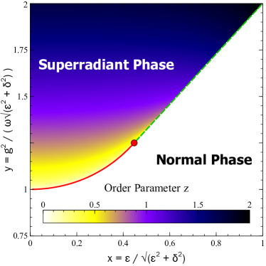
Figure 2: The phase diagram of the tricritical Dicke model. The order parameter $z$ vanishes in the normal phase and is finite in the superradiant phase. The quantum tricritical point (QTP) is marked by a red dot, which is located at the intersection of the second-order phase transition boundary (red solid line) and the first-order phase transition boundary (green dashed line).

While $H_{\mathrm{C}}$ determines the order parameter, $H_{\mathrm{Q}}$ in Eq. (10) gives the quantum fluctuation above the ground state, from which we can find the excitation gap and the ground state atom-light entanglement entropy. It is convenient to define the generalized position and momentum operators as

$$X_{i}=\frac{b_{i}+b_{i}^{{\dagger}}}{\sqrt{2\omega_{i}}},\,\;\;\;\;P_{i}=\sqrt{\frac{\omega_{i}}{2}}\frac{b_{i}-b_{i}^{{\dagger}}}{i}\,,\;\;\;i=1,2,3\,,$$

in terms of which, $H_{\mathrm{Q}}$ takes the form of a Hamiltonian that describes a 3-dimension harmonic oscillator:

$$H_{\mathrm{Q}} =\frac{1}{2}{\sum_{ij}P_{i}^{2}+\frac{1}{2}\left(\mathbf{\Omega}^{2}\right)_{ij}X_{i}X_{j}-}\frac{{\omega_{i}}}{{2}}\,,$$ (12)

$$\mathbf{\Omega}^{2} \mathbf{\equiv}\begin{pmatrix}\omega_{1}^{2}&\lambda_{12}&\lambda_{13}\\ \lambda_{12}&\omega_{2}^{2}&0\\ \lambda_{13}&0&\omega_{3}^{2}\end{pmatrix}\,,\;\;\lambda_{ij}\equiv\sqrt{\frac{\omega_{i}\omega_{j}}{2}}g\cos\theta_{j}\,.$$

Here $X_{1}$ and $P_{1}$ represent the original photonic degrees of freedom, while $X_{2,3}$ and $P_{2,3}$ represent the atomic degrees of freedom.

From Hamiltonian (12), it follows that the lowest excitation energy, i.e., the excitation gap, $\Delta$, is given by the smallest eigenvalue of $\mathbf{\Omega}$, and the ground state wave function $\Psi_{G}$ is a Gaussian of the form

$$\Psi_{G}\left(\mathbf{X}\right)=\left(\frac{\det\mathbf{\Omega}}{\pi^{3}}\right)^{1/4}\exp\left(-\frac{\Omega_{ij}X_{i}X_{j}}{2}\right)\,,$$ (13)

from which we can calculate the reduced density matrix of the light field by integrating out the atomic degrees of freedom:

$$\rho\left(X_{1},X_{1}^{\prime}\right)=C\exp\left(-\frac{1}{2}A_{+}\left(X_{1}^{2}+X_{1}^{\prime 2}\right)+A_{-}X_{1}X_{1}^{\prime}\right)\,,$$ (14)

where$\,A_{\pm}\equiv\frac{1}{2}\left(\Omega_{11}\pm\frac{\det\mathbf{\Omega}}{\Omega_{33}\Omega_{22}-\Omega_{23}^{2}}\right)$ and $C$ is a normalization factor. The von Neumann entropy, which measures the entanglement between the light and atoms, can be calculated as Lambert et al. (2004)

$$S\equiv-\mathrm{Tr}\left(\rho\ln\rho\right)=\frac{\gamma}{e^{\gamma}-1}-\ln\left(1-e^{-\gamma}\right)\,,$$ (15)

where $\gamma\equiv\cosh^{-1}\left(A_{+}/A_{-}\right)$. In the limit $\gamma\ll 1$, we have $S\approx 1-\ln\gamma$. We calculate $\Delta$ and $S$ numerically and display the results in Fig. 3. These two quantities, unlike the order parameter or $H_{\mathrm{C}}$ which only depends on $x$ and $y$, also depend on $\lambda\equiv\omega/\omega_{0}$ like $H_{\mathrm{Q}}$. Therefore the full diagram should be 3-dimensional. In Fig. 3, we plot $\Delta$ and $S$ on the $\left(x,y\right)$-plane for $\lambda=0.1,\,1,\,10$. Although it is difficult to distinguish the two phases (normal and superradiant) through $\Delta$ and $S$, the phase boundary is quite clear in the plots. On the 2nd-order phase transition boundary, the gap closes and the critical entanglement entropy diverges logarithmically. By contrast, on the 1st-order phase transition boundary, both $\Delta$ and $S$ have finite jumps across the phase boundary.

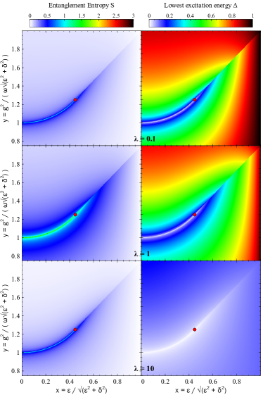
Figure 3: The atom-light entanglement entropy $S$ (left panel) and the lowest excitation energy $\Delta$ (right panel) as functions of $x$ and $y$ for $\lambda\equiv\omega/\omega_{0}=0.1$, 1, 10 (from top to bottom). The QTP is marked by the red dot as in Fig. 2.

Critical behavior — Let us now turn to the critical behavior of the tricritical Dicke model. One is often concerned with how the order parameter behaves near the critical line (i.e., the 2nd-order phase boundary). Consider a point $(x,y)$ in the superradiance region and close to the critical line, if we draw a line perpendicular to the critical line through this point and intercepts the critical line at $(x_{c},y_{c})$, then the order parameter at $\left(x,y\right)$ can be obtained by expanding $f(z)$ in powers of $z$

$$z^{2}=\frac{2\sqrt{y_{c}^{-2}+4x_{c}^{2}y_{c}^{2}}}{1-\allowbreak 5x_{c}^{2}\allowbreak\allowbreak}n+o\left(n\right)\,,$$ (16)

where $n$ is the distance between $\left(x,y\right)$ and the critical line. Hence, the critical exponent $\alpha$ defined by $z\propto n^{\alpha}$ is 1/2. However, if the line through $(x,y)$ intercepts the critical line at the QTP $(x_{tc},y_{tc})$, we have a different scaling:

$$z^{4}=\frac{5\sqrt{21}}{6}n\,+o\left(n\right),$$ (17)

which yields an exponent $\alpha=1/4$ for the QTP. In this sense, the QTP does not belong to the same universality class of the other critical points in this model, consistent with the general Landau theory of phase transition.

The critical behavior of the order parameter as described above is determined by $H_{\mathrm{C}}$. Now let us examine the behavior of the excitation gap $\Delta$ and the entanglement $S$, both of which are governed by $H_{\mathrm{Q}}$. To this end, we need to find the matrix elements of $\mathbf{\Omega}$. It can be shown that, on the critical line, $\mathbf{\Omega}$ has eigenvalues $0$, $\omega_{0}$ and $\sqrt{1+\lambda^{2}}\omega_{0}$. The smallest eigenvalue is $0$ which indicates that the gap $\Delta$ vanishes, as expected. Furthermore, the entropy $S$ diverges logarithmically according to Eq. (15). Near the critical line, to the leading order in $\det\left(\Omega/\omega_{0}\right)$, we have

$$\Delta/\omega_{0} \sim\left(1+\lambda^{2}\right)^{-1/2}\det\left(\Omega/\omega_{0}\right)\,,$$ (18)

$$S \sim 1-\frac{1}{2}\ln\left[\frac{4\left(\lambda^{2}+1\right)\det\left(\Omega/\omega_{0}\right)}{\lambda^{2}}\right]\,,$$ (19)

which establishes a universal relation between $S$ and $\Delta$ in the critical region as

$$S\sim 1-\frac{1}{2}\ln\left[\frac{4\left(\lambda^{2}+1\right)^{3/2}\Delta}{\lambda\omega_{0}}\right]\,.$$ (20)

Equation (20) represents another key result of this work. Two important remarks are in order here. First, Eq. (20) does not explicitly contain $z$, which is due to the separation of the classical and the quantum degrees of freedom aforementioned. The harmonic oscillator modes, depicted by $H_{\mathrm{Q}}$, are collective modes involving both light and atoms, emerging above the mean-field ground state of $H_{\mathrm{C}}$ in the thermodynamic limit, and Eq. (20) is solely determined by these modes, therefore we can call Eq. (20) an emergent quantum universality. Second, Eq. (20) is valid near all the critical points despite of the fact that points around the QTP exhibit different scaling behavior for the order parameter. It is even valid in the normal phase region below the critical line where the order parameter vanishes.

Given a point $(x,y)$ sufficiently close to, and a distance $n$ away from, the critical line, the key factor $\det\left(\Omega/\omega_{0}\right)$ in Eq. (19) can be expressed by $n$ as

$$\det\left(\Omega^{2}/\omega_{0}^{2}\right)/\lambda^{2}=\beta\sqrt{y_{c}^{-2}+4x_{c}^{2}y_{c}^{2}}\,n\,+o\left(n\right),$$ (21)

where the coefficient $\beta$ takes different values in different critical regions. If $(x,y)$ is located in the superradiant phase, then $\beta=2$ unless $(x,y)$ approaches the QTP, in which case $\beta=4$. If $(x,y)$ is located in the normal phase where $z=0$, then $\beta=1$. The scaling exponent between $\det\left(\Omega/\omega_{0}\right)$ and $n,$ is always the same while the scaling amplitude varies. Consequently, we have $\Delta\propto n^{1/2}$ and the entropy diverges logarithmically in terms of $n$. Another point to remark is that, as a function of $\lambda$, the critical entanglement entropy takes the form $S\left(\lambda\right)\approx-\frac{1}{2}\ln\left(\lambda+\lambda^{-1}\right)+\mathrm{const}$, which indicates that the entanglement between light and atom is maximized under the resonance condition $\lambda=1$.

In our model, as in the conventional Dicke model, the strengths of the rotating and the counter-rotating terms are equal. Previous studies have considered a Dicke-type model where these two strengths can have different values and found that there exists a multicritical point in the ground state phase diagram Baksic and Ciuti (2014). However, in the presence of dissipation, the multicritical point disappears Soriente et al. (2018). This is related to the disappearance of the superradiance phase in the presence of dissipation when the counter-rotating terms are absent. Due to the presence of the counter-rotating terms, we expect that the QTP in our model should be robust against dissipation. Nevertheless, how the dissipation affect the universal scaling requires further study.

Conclusion — In conclusion, we have constructed a generalized Dicke model that supports a QTP. The phase boundary and the position of the QTP in the parameter space, as well as the scaling behavior of the order parameter, can be determined from the mean-field theory and are found analytically. From this, we explicitly show that the QTP belongs to a different universality class than other points on the critical line. We further investigated the quantum fluctuations above the mean-field ground state, and calculated the excitation gap and the entanglement entropy and their critical behavior near the critical line. We established a new universal relation between the excitation gap and the entanglement entropy in the entire critical regime that includes the QTP. The universality is the result of the separation of the quantum and the classical degrees of freedom in the thermodynamic limit, being the property of the emergent collective quantum modes. Our model could be realized using atoms and cavities, or maybe other platforms, with current technology. Our work opens up new opportunities to investigate quantum tricriticality.

We acknowledge the support from the NSF and the Welch Foundation (Grant No. C-1669).

References

- Griffiths (1970) R. B. Griffiths, Phys. Rev. Lett. 24, 715 (1970).
- Chang et al. (1973) T. S. Chang, A. Hankey, and H. E. Stanley, Phys. Rev. B 8, 346 (1973).
- Riedel (1972) E. K. Riedel, Phys. Rev. Lett. 28, 675 (1972).
- Henkel (2013) M. Henkel, Conformal Invariance and Critical Phenomena (Springer-Verlag Berlin Heidelberg, 2013).
- Sachdev (2011) S. Sachdev, Quantum phase transitions (Cambridge university press, 2011).
- Kaluarachchi et al. (2018) U. S. Kaluarachchi, V. Taufour, S. L. Bud’ko, and P. C. Canfield, Phys. Rev. B 97, 045139 (2018).
- Friedemann et al. (2018) S. Friedemann, W. J. Duncan, M. Hirschberger, T. W. Bauer, R. Küchler, A. Neubauer, M. Brando, C. Pfleiderer, and F. M. Grosche, Nature Physics 14, 62 (2018).
- Dicke (1954) R. H. Dicke, Phys. Rev. 93, 99 (1954).
- Garraway (2011) B. M. Garraway, Phil. Trans. R. Soc. A 369, 1137 (2011).
- Dimer et al. (2007) F. Dimer, B. Estienne, A. S. Parkins, and H. J. Carmichael, Phys. Rev. A 75, 013804 (2007).
- Nagy et al. (2010) D. Nagy, G. Kónya, G. Szirmai, and P. Domokos, Phys. Rev. Lett. 104, 130401 (2010).
- Baumann et al. (2010) K. Baumann, C. Guerlin, F. Brennecke, and T. Esslinger, Nature 464, 1301 (2010).
- Zhang et al. (2018) Z. Zhang, C. H. Lee, R. Kumar, K. J. Arnold, S. J. Masson, A. L. Grimsmo, A. S. Parkins, and M. D. Barrett, Phys. Rev. A 97, 043858 (2018).
- Lamata (2017) L. Lamata, Scientific Reports 7, 43768 (2017).
- Mezzacapo et al. (2014) A. Mezzacapo, U. Las Heras, J. Pedernales, L. DiCarlo, E. Solano, and L. Lamata, Scientific Reports 4, 7482 (2014).
- Langford et al. (2017) N. Langford, R. Sagastizabal, M. Kounalakis, C. Dickel, A. Bruno, F. Luthi, D. Thoen, A. Endo, and L. DiCarlo, Nature Communications 8, 1715 (2017).
- Li et al. (2018) X. Li, M. Bamba, N. Yuan, Q. Zhang, Y. Zhao, M. Xiang, K. Xu, Z. Jin, W. Ren, G. Ma, S. Cao, D. Turchinovich, and J. Kono, Science 361, 794 (2018).
- Wang and Hioe (1973) Y. K. Wang and F. T. Hioe, Phys. Rev. A 7, 831 (1973).
- Lambert et al. (2004) N. Lambert, C. Emary, and T. Brandes, Phys. Rev. Lett. 92, 073602 (2004).
- Lambert et al. (2005) N. Lambert, C. Emary, and T. Brandes, Phys. Rev. A 71, 053804 (2005).
- Pyrkov and Byrnes (2013) A. N. Pyrkov and T. Byrnes, New Journal of Physics 15, 093019 (2013).
- Ortiz et al. (2018) S. Ortiz, Y. Song, J. Wu, V. Ivannikov, and T. Byrnes, Phys. Rev. A 98, 043616 (2018).
- Wakayama (2017) M. Wakayama, Journal of Physics A: Mathematical and Theoretical 50, 174001 (2017).
- Niemczyk et al. (2010) T. Niemczyk, F. Deppe, H. Huebl, E. Menzel, F. Hocke, M. Schwarz, J. Garcia-Ripoll, D. Zueco, T. Hümmer, E. Solano, et al., Nature Physics 6, 772 (2010).
- Holstein and Primakoff (1940) T. Holstein and H. Primakoff, Phys. Rev. 58, 1098 (1940).
- Note (1) Following the standard procedure, we obtain the mean-field Hamiltonian by replacing the bosonic operator in the Hamiltonian , Eq. (1) with its expectation value : , with . The mean-field ground state is reached when the -th atom is polarized along the direction anti-parallel to , with the corresponding mean-field energy functional , which yields in Eq. (5) of the text.
- Note (2) Writing as a power series of : , we can extract the coefficients of the series and analytically obtain the equations which determines phase boundary and the tricritical point. For example, the critical line (2nd-order phase transition boundary) is determined by which yields . The QTP is determined by , which yields Eq. (11) of the text.
- Baksic and Ciuti (2014) A. Baksic and C. Ciuti, Phys. Rev. Lett. 112, 173601 (2014).
- Soriente et al. (2018) M. Soriente, T. Donner, R. Chitra, and O. Zilberberg, Phys. Rev. Lett. 120, 183603 (2018).