Integer Programming for Learning Directed Acyclic Graphs from Continuous Data
Abstract
Learning directed acyclic graphs (DAGs) from data is a challenging task both in theory and in practice, because the number of possible DAGs scales superexponentially with the number of nodes. In this paper, we study the problem of learning an optimal DAG from continuous observational data. We cast this problem in the form of a mathematical programming model which can naturally incorporate a super-structure in order to reduce the set of possible candidate DAGs. We use the penalized negative log-likelihood score function with both and regularizations and propose a new mixed-integer quadratic optimization (MIQO) model, referred to as a layered network (LN) formulation. The LN formulation is a compact model, which enjoys as tight an optimal continuous relaxation value as the stronger but larger formulations under a mild condition. Computational results indicate that the proposed formulation outperforms existing mathematical formulations and scales better than available algorithms that can solve the same problem with only regularization. In particular, the LN formulation clearly outperforms existing methods in terms of computational time needed to find an optimal DAG in the presence of a sparse super-structure.
1 Introduction
The study of Probabilistic Graphical Models (PGMs) is an essential topic in modern artificial intelligence [23]. A PGM is a rich framework that represents the joint probability distribution and dependency structure among a set of random variables in the form of a graph. Once learned from data or constructed from expert knowledge, PGMs can be utilized for probabilistic reasoning tasks, such as prediction; see [23, 24] for comprehensive reviews of PGMs.
Two most common classes of PGMs are Markov networks (undirected graphical models) and Bayesian networks (directed graphical models). A Bayesian Network (BN) is a PGM in which the conditional probability relationships among random variables are represented in the form of a Directed Acyclic Graph (DAG). BNs use the richer language of directed graphs to model probabilistic influence among random variables that have clear directionality; they are particularly popular in practice, with applications in genetics [45], biology [27], machine learning [23], and causal inference [39].
Learning BNs is a central problem in machine learning. An essential part of this problem entails learning the DAG structure that accurately represents the (hypothetical) joint probability distribution of the BN. Although one can form the DAG based on expert knowledge, acquisition of knowledge from experts is often costly and nontrivial. Hence, there has been considerable interest in learning the DAG directly from observational data [3, 6, 9, 10, 17, 29, 34, 39].
Learning the DAG which best explains observed data is an NP-hard problem [5]. Despite this negative theoretical result, there has been interest in developing methods for learning DAGs in practice. There are two main approaches for learning DAGs from observational data: constraint-based and score-based. In constraint-based methods, such as the well-known PC-Algorithm [39], the goal is to learn a completed partially DAG (CPDAG) consistent with conditional independence relations inferred from the data. Score-based methods, including the approach in this paper, aim to find a DAG that maximizes a score that measures how well the DAG fits the data.
Existing DAG learning algorithms can also be divided into methods for discrete and continuous data. Score-based methods for learning DAGs from discrete data typically involve a two-stage learning process. In stage 1, the score for each candidate parent set (CPS) of each node is computed. In stage 2, a search algorithm is used to maximize the global score, so that the resulting graph is acyclic. Both of these stages require exponential computation time [42]. For stage 2, there exist elegant exact algorithms based on dynamic programming [13, 21, 22, 30, 32, 36, 44], A⋆ algorithm [43, 44], and integer-programming [2, 3, 7, 8, 9, 10]. The A⋆ algorithm identifies the optimal DAG by solving a shortest path problem in an implicit state-space search graph, whereas integer programming (IP) directly casts the problem as a constrained optimization problem. Specifically, the variables in the IP model indicate whether or not a given parent set is assigned to a node in the network. Hence, the problem involves binary variables for nodes. To reduce the number of binary variables, a common practice is to limit the cardinality of each parent set [3, 9], which can lead to suboptimal solutions.
A comprehensive empirical evaluation of A⋆ algorithm and IP methods for discrete data is conducted in [26]. The results show that the relative efficiency of these methods varies due to the intrinsic differences between them. In particular, state-of-the-art IP methods can solve instances up to 1,000 CPS per variable regardless of the number of nodes, whereas A⋆ algorithm works for problems with up to 30 nodes, even with tens of thousands of CPS per node.
While statistical properties of DAG learning from continuous data have been extensively studied [15, 25, 34, 37, 41], the development of efficient computational tools for learning the optimal DAG from continuous data remains an open challenge. In addition, despite the existence of elegant exact search algorithms for discrete data, the literature on DAG learning from continuous data has primarily focused on approximate algorithms based on coordinate descent [14, 17] and non-convex continuous optimization [46]. To our knowledge, [29] and [42] provide the only exact algorithms for learning medium to large DAGs from continuous data. An IP-based model using the topological ordering of variables is proposed in [29]. An A⋆-lasso algorithm for learning an optimal DAG from continuous data with an regularization is developed in [42]. A⋆-lasso incorporates the lasso-based scoring method within dynamic programming to avoid an exponential number of parent sets and uses the A⋆ algorithm to prune the search space of the dynamic programming method.
Given the state of existing algorithms for DAG learning from continuous data, there is currently a gap between theory and computation: While statistical properties of exact algorithms can be rigorously analyzed [25, 41], it is much harder to assess the statistical properties of approximate algorithms [1, 14, 17, 46] that offer no optimality guarantees [21]. This gap becomes particularly noticeable in cases where the statistical model is identifiable from observational data. In this case, the optimal score from exact search algorithms is guaranteed to reveal the true underlying DAG when the sample size is large. Therefore, causal structure learning from observational data becomes feasible [25, 33].
In this paper, we focus on DAG learning for an important class of BNs for continuous data, where causal relations among random variables are linear. More specifically, we consider DAGs corresponding to linear structural equations models (SEMs). In this case, network edges are associated with the coefficients of regression models corresponding to linear SEMs. Consequently, the score function can be explicitly encoded as a penalized negative log-likelihood function with an appropriate choice of regularization [29, 35, 41]. Hence, the process of computing scores (i.e., stage 1) is completely bypassed, and a single-stage model can be formulated [42]. Moreover, in this case, IP formulations only require a polynomial, rather than exponential, number of variables, because each variable can be defined in the space of arcs instead of parent sets. Therefore, cardinality constraints on the size of parent sets, which are used in earlier methods to reduce the search space and may lead to suboptimal solutions, are no longer necessary.
Contributions
In this paper, we develop tailored exact DAG learning methods for continuous data from linear SEMs, and make the following contributions:
-
–
We develop a mathematical framework that can naturally incorporate prior structural knowledge, when available. Prior structural knowledge can be supplied in the form of an undirected and possibly cyclic graph (super-structure). An example is the skeleton of the DAG, obtained by removing the direction of all edges in a graph. Another example is the moral graph of the DAG, obtained by adding an edge between pairs of nodes with common children and removing the direction of all edges [39]. The skeleton and moral graphs are particularly important cases, because they can be consistently estimated from observational data under proper assumptions [20, 25]. Such prior information limits the number of possible DAGs and improves the computational performance.
-
–
We discuss three mathematical formulations, namely, cutting plane (CP), linear ordering (LO), and topological ordering (TO) formulations, for learning an optimal DAG, using both and -penalized likelihood scores. We also propose a new mathematical formulation to learn an optimal DAG from continuous data, the layered network (LN) formulation, and establish that other DAG learning formulations entail a smaller continuous relaxation feasible region compared to that of the continuous relaxation of the LN formulation (Propositions 3 and 4). Nonetheless, all formulations attain the same optimal continuous relaxation objective function value under a mild condition (Propositions 5 and 6). Notably, the number of binary variables and constraints in the LN formulation solely depend on the number of edges in the super-structure (e.g., moral graph). Thus, the performance of the LN formulation substantially improves in the presence of a sparse super-structure. The LN formulation has a number of other advantages; it is a compact formulation in contrast to the CP formulation; its relaxation can be solved much more efficiently compared with the LO formulation; and it requires fewer binary variables and explores fewer branch-and-bound nodes than the TO formulation. Our empirical results affirm the computational advantages of the LN formulation. They also demonstrate that the LN formulation can find a graph closer to the true underlying DAG. These improvements become more noticeable in the presence of a prior super-structure (e.g., moral graph).
-
–
We compare the IP-based method and the A⋆-lasso algorithm for the case of regularization. As noted earlier, there is no clear winner among A⋆-style algorithms and IP-based models for DAG learning from discrete data [26]. Thus, a wide range of approaches based on dynamic programming, A⋆ algorithm, and IP-based models have been proposed for discrete data. In contrast, for DAG learning from continuous data with complete super-structure, the LN formulation remains competitive with the state-of-art A⋆-lasso algorithm for small graphs, whereas it performs better for larger problems. Moreover, LN performs substantially better when a sparse super-structure is available. This is mainly because the LN formulation directly defines the variables based on the super-structure, whereas the A⋆-lasso algorithm cannot take advantage of the prior structural knowledge as effectively as the LN formulation.
In Section 2, we outline the necessary preliminaries, define the DAG structure learning problem, and present a general framework for the problem. Mathematical formulations for DAG learning are presented in Section 3. The strengths of different optimization problems are discussed in Section 4. Empirical results are presented in Sections 5 and 6. We end the paper with a summary and discussion of future research in Section 7.
2 Penalized DAG Estimation with Linear SEMs
The causal effect of (continuous) random variables in a DAG can be described by SEMs that represent each variable as a (nonlinear) function of its parents. The general form of these models is given by [31]
| (1) |
where is the random variable associated with node ; denotes the parents of node in , i.e., the set of nodes with arcs pointing to node ; is the number of nodes; and latent random variables, represent the unexplained variation in each node.
An important class of SEMs is defined by linear functions, , which can be described by linear regressions of the form
| (2) |
where represents the effect of node on for . In the special case where the random variables are Gaussian, Equations (1) and (2) are equivalent, in the sense that are coefficients of the linear regression model of on , , and for [35]. However, estimation procedures proposed in this paper are not limited to Gaussian random variables and apply more generally to linear SEMs [25, 35].
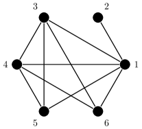
Let be an undirected and possibly cyclic super-structure graph with node set and edge set . From , generate a bi-directional graph where . Throughout the paper, we refer to directed edges as arcs and to undirected edges as edges.
Consider i.i.d. observations from the linear SEM (2). Let be the data matrix with rows representing i.i.d. samples, and columns representing random variables. The linear SEM (2) can be compactly written as
| (3) |
where is a matrix with for and for all ; is the noise matrix. More generally, defines a directed graph on nodes such that arc appears in if and only if .
Let denote the variance of . We assume that all noise variables have equal variances, i.e., . This condition implies the identifiability of DAGs from Gaussian [33] and non-Gaussian [25] data. Under this condition, the negative log likelihood for linear SEMs with Gaussian or non-Gaussian noise is proportional to
| (4) |
where and is the identity matrix [25].
In practice, we are often interested in learning sparse DAGs. Thus, a regularization term is used to obtain a sparse estimate. For the linear SEM (2), the optimization problem corresponding to the penalized negative log-likelihood with super-structure (PNL) for learning sparse DAGs is given by
| PNL | (5a) | |||
| s.t., | (5b) | |||
The objective function (5a) consists of two parts: the quadratic loss function, , from (4), and the regularization term, . Popular choices for include -regularization or lasso [40], , and -regularization, , where if , and 0 otherwise. The tuning parameter controls the degree of regularization. The constraint (5b) stipulates that the resulting directed subgraph (digraph) has to be an induced DAG from .
When the super-structure is a complete graph, PNL reduces to the classical PNL. In this case, the consistency of sparse PNL for DAG learning from Gaussian data with an penalty follows from an analysis similar to [41]. In particular, we have
where is the estimate of the true structure . An important advantage of the PNL estimation problem is that its consistency does not require the (strong) faithfulness assumption [33, 41].
The mathematical model (5) incorporates a super-structure (e.g., moral graph) into the PNL model. When is the moral graph, the consistency of sparse PNL follows from the analysis in [25], which studies the consistency of the following two-stage framework for estimating sparse DAGs: (1) infer the moral graph from the support of the inverse covariance matrix; and (2) choose the best-scoring induced DAG from the moral graph. The authors investigate conditions for identifiability of the underlying DAG from observational data and establish the consistency of the two-stage framework.
3 Mathematical Formulations
Prior to presenting mathematical formulations for solving PNL, we discuss a property of DAG learning from continuous data that distinguishes it from the corresponding problem for discrete data. To present this property in Proposition 1, we need a new definition.
Definition 1.
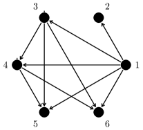
A tournament is a directed graph obtained by specifying a direction for each edge in the super-structure graph (see Figure 1).
Proposition 1.
There exists an optimal solution to PNL (5) with an (or an ) regularization that is a cycle-free tournament.
All proofs are given in Appendix I. Proposition 1 implies that for DAG learning from continuous variables, the search space reduces to acyclic tournament structures. This is a far smaller search space when compared with the super-exponential search space of DAGs for discrete variables. However, one has to also identify the optimal parameters. This search for optimal parameters is critical, as it further reduces the super-structure to the edges of the DAG by removing the edges with zero coefficients.
A solution method based on brute force enumeration of all tournaments requires computational time when is complete, where denotes the computational time associated with solving PNL given a known tournament structure. This is because when is complete, the total number of tournaments (equivalently the total number of permutations) is . However, when is incomplete, the number of DAGs is fewer than . The topological search space is regardless of the structure of and several topological orderings can correspond to the same DAG. The TO formulation [29] is based on this search space. In Section 3.2, we discuss a search space based on the layering of a DAG, which uniquely identifies a DAG, and propose the corresponding Layered Network (LN) formulation, which effectively utilizes the structure of . We first discuss existing mathematical formulations for the PNL optimization problem (5) in the next section. Given the desirable statistical properties of regularization [41] and the fact that existing mathematical formulations are given for regularization, we present the formulations for regularization. We outline the necessary notation below.
Indices
: index set of random variables
: index set of samples
Input
: an undirected super-structure graph (e.g., the moral graph)
: the bi-directional graph corresponding to the undirected graph
, where and denotes th sample () of random variable
tuning parameter (penalty coefficient)
Continuous optimization variables
: weight of arc representing the regression coefficients
Binary optimization variables
3.1 Existing Mathematical Models
The main source of difficulty in solving PNL is due to the acyclic nature of DAG imposed by the constraint in (5b). A popular technique for ensuring acyclicity is to use cycle elimination constraints, which were first introduced in the context of the Traveling Salesman Problem (TSP) in [11].
Let be the set of all possible cycles and be the set of arcs defining a cycle and define . Then, the -PNL model can be formulated as
| (6a) | |||||
| (6b) | |||||
| (6c) | |||||
| (6d) | |||||
Following [29], the objective function (6a) is an expanded version of in PNL (multiplied by ) with an regularization. The constraints in (6b) stipulate that only if , where is a sufficiently large constant. The constraints in (6c) rule out all cycles. Note that for , constraints in (6c) ensure that at most one arc exists among two nodes. The last set of constraints specifies the binary nature of the decision vector . Note that variables are continuous and unrestricted; however, in typical applications, they can be bounded by a finite number . This formulation requires binary variables and an exponential number of constraints. A cutting plane method [28] that adds the cycle elimination inequalities as needed is often used to solve this problem. We refer to this formulation as the cutting plane (CP) formulation.
Remark 1.
For a complete super-structure , it suffices to impose the set of constraints in (6c) only for cycles of size 2 and 3 given by
In other words, the CP formulation (both with and regularizations) needs a polynomial number of constraints for complete super-structure .
The second formulation is based on a well-known combinatorial optimization problem, known as linear ordering (LO) [16]. Given a finite set with elements, a linear ordering of is a permutation where denotes the set of all permutations with elements. In the LO problem, the goal is to identify the best permutation among nodes. The “cost” for a permutation depends on the order of the elements in a pairwise fashion. Let denote the order of node in permutation . Then, for two nodes , the cost is if the order of node precedes the order of node () and is otherwise (). A binary variable indicates whether . Because and , one only needs variables to cast the LO problem as an IP formulation [16].
The LO formulation for DAG learning from continuous data has two noticeable differences compared with the classical LO problem: (i) the objective function is quadratic, and (ii) an additional set of continuous variables, i.e., s, is added. Cycles are ruled out by directly imposing the linear ordering constraints. The PNL can be formulated as (8).
| (8a) | |||||
| (8b) | |||||
| (8c) | |||||
| (8d) | |||||
| (8e) | |||||
| (8f) | |||||
| (8g) | |||||
The interpretation of constraints (8b)-(8d) is straightforward. The constraints in (8c) imply that if node appears after node in a linear ordering (), then there should not exist an arc from to (). The set of inequalities (8e) implies that if and , then . This ensures the linear ordering of nodes and removes cycles.
The third approach for ruling out cycles is to impose a set of constraints such that the nodes follow a topological ordering. A topological ordering is a linear ordering of the nodes of a graph such that the graph contains an arc if node appears before node in the linear order. Define decision variables for all . This variable takes value 1 if topological order of node (i.e., ) equals , and 0, otherwise. If a topological ordering is known, the DAG structure can be efficiently learned in polynomial time [35], but the problem remains challenging when the ordering is not known. The topological ordering prevents cycles in the graph. This property is used in [29] to model the problem of learning a DAG with regularization. We extend their formulation to regularization. The topological ordering (TO) formulation is given by
| (9a) | |||||
| (9b) | |||||
| (9c) | |||||
| (9d) | |||||
| (9e) | |||||
| (9f) | |||||
| (9g) | |||||
| (9h) | |||||
| (9i) | |||||
| (9j) | |||||
In this formulation, is an auxiliary binary variable which takes value 1 if an arc exists from node to node . Recall that, if . The constraints in (9c) enforce the correct link between and , i.e., has to take value zero if . The constraints in (9d) imply that there should not exist a bi-directional arc among two nodes. This inequality can be replaced with equality (Corollary 1). The constraints in (9e) remove cycles by imposing an ordering among nodes. The set of constraints in (9f)-(9g) assigns a unique topological order to each node. The last two sets of constraints indicate the binary nature of decision variables and .
Corollary 1, which is a direct consequence of Proposition 1, implies that we can use for all and reduce the number of binary variables.
Corollary 1.
The constraints in (9d) can be replaced by .
In constraints (9b)-(9i), both variables and are needed to correctly model the regularization term in the objective function (see Figure 2(a)). This is because the constraints (9e) satisfy the transitivity property: if for and for , then for , since implies that ; similarly, implies . If we sum both inequalities, we have , which enforces . Such a transitivity relation, however, need not hold for the decision vector . In other words, the decision variable is used to keep track of the number of non-zero weights associated with the arc , and the decision vector is used to remove cycles via the set of constraints in (9e) by creating an acyclic tournament on the super-structure . A tournament on super-structure assigns a direction for each edge in an undirected super-structure . In other words, if we were to let for and hence use the decision variable in the objective, then we would be counting the number of edges, equal to , instead of number of non-zero values.
3.2 A New Mathematical Model: The Layered Network (LN) Formulation
As an alternative to the existing mathematical formulations, we propose a new formulation for imposing acyclicity constraints that is motivated by the layering of nodes in DAGs [18]. More specifically, our formulation ensures that the resulting graph is a layered network, in the sense that there exists no arc from a layer to layer , where . Let be the layer value for node . One may interpret as for all , where the variables are as defined in the TO formulation. However, note that the notion of is more general because need not be integer. Figure 3 depicts the layered network encoding of a DAG. With this notation, our layered network (LN) formulation can be written as
| (10a) | |||||
| (10b) | |||||
| (10c) | |||||
| (10d) | |||||
| (10e) | |||||
| (10f) | |||||
| (10g) | |||||
| (10h) | |||||
The interpretation of the constraints (10b)-(10c) is straightforward. The constraints in (10e) ensure that the graph is a layered network. The last set of constraints indicates the continuous nature of the decision variable and gives the tightest valid bound for . It suffices to consider any real number for layer values as long as layer values of any two nodes differ by at least one if there exists an arc between them. Additionally, LN uses a tighter inequality compared to TO, by replacing with parameter in (10e). This is because the difference between the layer values of two nodes can be at most for a DAG with nodes. The next proposition establishes the validity of the LN formulation.
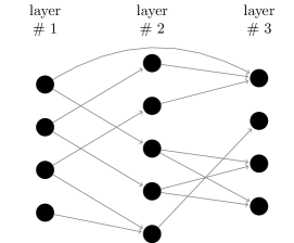
The LN formulation highlights a desirable property of the layered network representation of a DAG in comparison to the topological ordering representation. Let us define nodes in layer 1 as the set of nodes that have no incoming arcs in the DAG, nodes in layer 2 as the set of nodes that have incoming arcs only from nodes in the layer 1, layer 3 as the set of nodes that have incoming arcs from layer 2 (and possibly layer 1), etc. (see Figure 3). The minimal layer number of a node is the length of the longest directed path from any node in layer 1 to that node. For a given DAG, there is a unique minimal layer number, but not a unique topological order. As an example, Figure 2(a) has three valid topological orders: (i) 1,2,4,3, (ii) 1,4,2,3, and (iii) 4,1,2,3. In contrast, it has a unique layer representation, 1,2,3,1.
There is a one-to-one correspondence between minimal layer numbering and a DAG. However, the solutions of the LN formulation, i.e., variables (layer values), do not necessarily correspond to the minimal layer numbering. This is because the LN formulation does not impose additional constraints to enforce a minimal numbering and can output solutions that are not minimally numbered. However, because branch-and-bound does not branch on continuous variables, alternative (non-minimal) feasible solutions for the variables do not impact the branch-and-bound process. On the contrary, we have multiple possible representations of the same DAG with topological ordering. Because topological ordering variables are binary, the branch-and-bound method applied to the TO formulation explores multiple identical DAGs as it branches on the topological ordering variables. This enlarges the size of the branch-and-bound tree and increases the computational burden.
Layered network representation also has an important practical implication: Using this representation, the search space can be reduced to the total number of ways we can layer a network (or equivalently the total number of possible minimal layer numberings) instead of the total number of topological orderings. When the super-structure is complete, both quantities are the same, and equal to . Otherwise, a brute-force search for finding the optimal DAG has computational time , where denotes the total number of minimal layered numberings, and is the computational complexity of solving PNL given a known tournament structure.
We close this section by noting that a set of constraints similar to (10e) was introduced in [7] for learning pedigree. However, the formulation in [7] requires an exponential number of variables. In more recent work on DAGs for discrete data, Cussens and colleagues have focused on a tighter formulation for removing cycles, known as cluster constraints [8, 9, 10]. To represent the set of cluster constraints, variables have to be defined according to the parent set choice leading to an exponential number of variables. Thus, such a representation is not available in the space of arcs.
3.2.1 Layered Network with regularization
Because of its convexity, the structure learning literature has utilized the -regularization for learning DAGs from continuous variables [17, 29, 35, 42, 46]. The LN formulation with -regularization can be written as
| (11a) | |||||
| (11b) | |||||
Remark 2.
For a complete super-structure , . Thus, the LN formulations (both and ) can be encoded without variables by writing (10e) as
Remark 3.
CP and LO formulations reduce to the same formulation for regularization when the super-structure is complete by letting in formulation (8) for all .
| Incomplete (moral) | Complete (moral) | ||||||||
| CP | LO | TO | LN | CP | LO | TO | LN | ||
| Binary Vars () | |||||||||
| Binary Vars () | |||||||||
| Constraints | |||||||||
| (both and ) | Exp | 2 | 2 | ||||||
An advantage of the -regularization for DAG learning is that all models (CP, LO, TO and LN) can be formulated without decision variables , since counting the number of non-zero is no longer necessary.
Table 1 shows the number of binary variables and the number of constraints associated with cycle prevention constraints in each model. Evidently, models require additional binary variables compared to the corresponding models. Note that the number of binary variables and constraints for the LN formulation solely depend on the number of edges in the super-structure . This property is particularly desirable when the super-structure is sparse. The LN formulation requires the fewest number of constraints among all models. The LN formulation also requires fewer binary variables than the TO formulation. More importantly, different topological orders for the same DAG are symmetric solutions to the associated TO formulation. Consequently, branch-and-bound requires exploring multiple symmetric formulations as it branches on fractional TO variables. As for the LO formulation, the number of constraints is which makes its continuous relaxation cumbersome to solve in the branch-and-bound process. The LN formulation is compact, whereas the CP formulation requires an exponential number of constraints for incomplete super-structure . The CP formulation requires fewer binary variables for formulation than LN; both formulations need the least number of binary variables for regularization.
In the next section, we discuss the theoretical strength of these mathematical formulations and provide a key insight on why the LN formulation performs well for learning DAGs from continuous data.
4 Continuous Relaxation
One of the fundamental concepts in IP is relaxations, wherein some or all constraints of a problem are loosened. Relaxations are often used to obtain a sequence of easier problems which can be solved efficiently yielding bounds and approximate, not necessarily feasible, solutions for the original problem. Continuous relaxation is a common relaxation obtained by relaxing the binary variables of the original mixed-integer quadratic program (MIQP) and allowing them to take real values. Continuous relaxation is at the heart of branch-and-bound methods for solving MIQPs. An important concept when comparing different MIQP formulations is the strength of their continuous relaxations.
Definition 2.
A formulation is said to be stronger than formulation if where and correspond to the feasible regions of continuous relaxations of and , respectively.
Proposition 3.
The LO formulation is stronger than the LN formulation, that is,
.
Proposition 4.
When the parameter in (9e) is replaced with , the TO formulation is stronger than the LN formulation, that is, .
These propositions are somewhat expected because the LN formulation uses the fewest number of constraints. Hence, the continuous relaxation feasible region of the LN formulation is loosened compared to the other formulations. The next two results justify the advantages of the LN formulation.
Proposition 5.
Let denote the optimal coefficient associated with an arc from (5). For both and regularizations, the initial continuous relaxations of the LN formulation attain as tight an optimal objective function value as the LO, CP, TO formulations if .
Proposition 5 states that although the LO and TO formulations are tighter than the LN formulation with respect to the feasible region of their continuous relaxations, the continuous relaxation of all models attain the same objective function value (root relaxation).
Proposition 6.
For the same variable branching in the branch-and-bound process, the continuous relaxations of the LN formulation for both and regularizations attain as tight an optimal objective function value as LO, CP and TO, if .
Proposition 6 is at the crux of this section. It shows that not only does the tightness of the optimal objective function value of the continuous relaxation hold for the root relaxation, but it also holds throughout the branch-and-bound process under the specified condition on , if the same branching choices are made. Thus, the advantages of the LN formulation are due to the fact that it is a compact formulation that entails the fewest number of constraints, while attaining the same optimal objective value of continuous relaxation as tighter models.
5 Comparison of MIQP Formulations
We present numerical results comparing the proposed LN formulation with existing approaches. Experiments are performed on a cluster operating on UNIX with Intel Xeon E5-2640v4 2.4GHz. All MIQP formulations are implemented in the Python programming language. Gurobi 8.0 is used as the MIQP solver. A time limit of (in seconds), where denotes the number of nodes, is imposed across all experiments after which runs are aborted. Unless otherwise stated, an MIQP optimality gap of is imposed across all experiments; the gap is calculated by where UB denotes the objective value associated with the best feasible integer solution (incumbent) and LB represents the best obtained lower bound during the branch-and-bound process.
For CP, instead of incorporating all constraints given by (6c), we begin with no constraint of type (6c). Given an integer solution with cycles, we detect a cycle and impose a new cycle prevention constraint to remove the detected cycle. Depth First Search (DFS) can detect a cycle in a directed graph with complexity . Gurobi Lazy Callback is used, which allows adding cycle prevention constraints in the branch-and-bound algorithm, whenever an integer solution with cycles is found. The same approach is used by [29]. Note that Gurobi solver follows a branch-and-cut implementation and adds many general-purpose and special-purpose cutting planes.
To select the parameter in all formulations we use the proposal of [29]. Specifically, given , we solve each problem without cycle prevention constraints. We then use the upper bound . The results provided in [29] computationally confirm that this approach gives a large enough value of . We also confirmed the validity of this choice across all our test instances.
5.1 Synthetic datasets
We use the R package pcalg to generate random Erdős-Rényi graphs. Firstly, we create a DAG using randomDAG function and assign random arc weights (i.e., ) from a uniform distribution, . This ground truth DAG is used to assess the quality of estimates. Next, the resulting DAG and random coefficients are input to the rmvDAG function, which uses linear regression as the underlying model, to generate multivariate data (columns of matrix ) with the standard normal error distribution.
We consider nodes and samples. The average outgoing degree of each node, denoted by , is set to 2. We generate 10 random graphs for each setting (, , ). The raw observational data, , for the datasets with is the same as first 100 rows of the datasets with .
We consider two types of problem instances: (i) a set of instances for which the moral graph corresponding to the true DAG is available; (ii) a set of instances with a complete undirected graph, i.e., assuming no prior knowledge. The first class of problems is referred to as moral instances, whereas the second class is called complete instances. The raw observational data, , for moral and complete instances are the same. The function moralize(graph) in the pcalg R-package is used to generated the moral graph from the true DAG. The moral graph can also be (consistently) estimated from data using penalized estimation procedures with polynomial complexity [20, 25]. However, since the quality of the moral graph equally affects all optimization models, the true moral graph is used in our experiments.
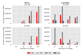
We use the following IP-based metrics to measure the quality of a solution: Optimality gap (MIQP GAP), computation time in seconds (Time), Upper Bound (UB), Lower Bound (LB), computational time of root continuous relaxation (Time LP), and the number of explored nodes in the branch-and-bound tree.
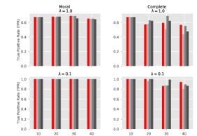
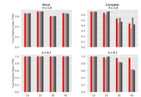
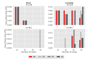
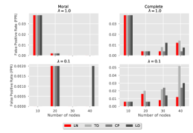
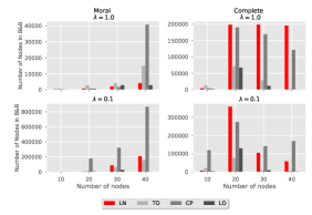
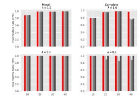
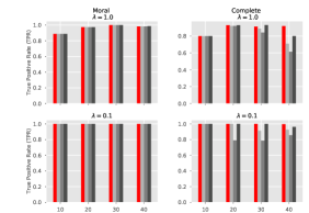
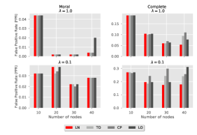
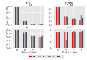
We also evaluate the quality of the estimated DAGs by comparing them with the ground truth. To this end, we use the average structural Hamming distance , as well as true positive (TPR) and false positive rates (FPR). These criteria evaluate different aspects of the quality of the estimated DAGs: counts the number of differences (addition, deletion, or arc reversal) required to transform predicted DAG to the true DAG; TPR is the number of correctly identified arcs divided by the total number of true arcs, ; FPR is the number of incorrectly identified arcs divided by the total number of negatives (non-existing arcs), . For brevity, TPR and FPR plots are presented in Appendix II.
5.2 Comparison of formulations
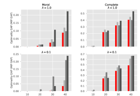
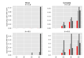
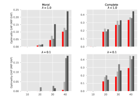
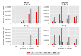
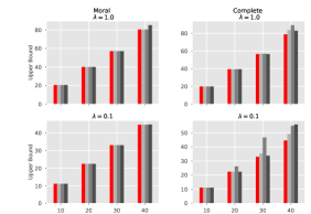
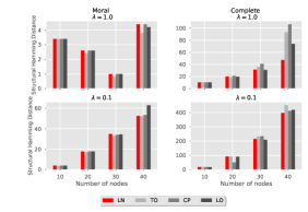
Figure 5 reports the average metrics across 10 random graphs for formulations with . The LO formulation fails to attain a reasonable solution for one graph (out of 10) with and . This is due to the large computation time for solving its continuous relaxation. We excluded these two instances from LO results.
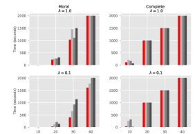
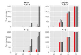
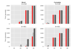
Figure 5(a) shows that the LN formulation outperforms other formulations in terms of the average optimality gap across all number of nodes and regularization parameters, . The difference becomes more pronounced for moral instances. For moral instances, the number of binary variables and constraints for LN solely depends on the size of moral graph. Figure 5(b) also indicates that the LN formulation requires the least computational time for small instances, whereas all models hit the time limit for larger instances.
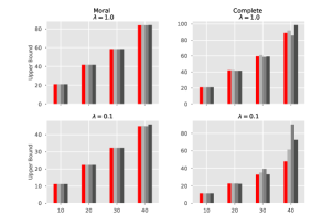
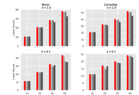
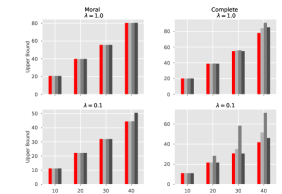
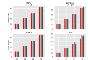
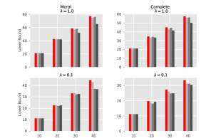
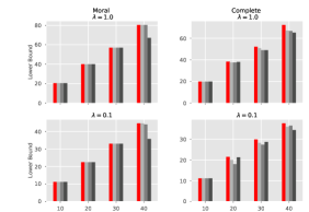
Figures 5(c)-(d) show the performance of all methods in terms of their upper and lower bounds. For easier instances (e.g., complete instances with and moral instances), all methods attain almost the same upper bound. Nonetheless, LN performs better in terms of improving the lower bound. For more difficult instances, LN outperforms other methods in terms of attaining a smaller upper bound (feasible solution) and a larger lower bound.
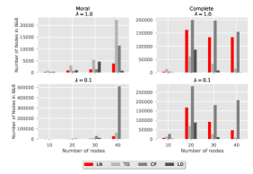
Figures 5(e)-(f) show the continuous relaxation time of all models, and the number of explored nodes in the branch-and-bound tree, respectively. The fastest computational time for the continuous relaxation is for the TO formulation followed by the LN formulation. However, the number of explored nodes provides more information about the performance of mathematical formulations. In small instances, i.e., , where an optimal solution is attained, the size of the branch-and-bound tree for the LN formulation is smaller than the TO formulation. This is because the TO formulation has a larger number of binary variables, leading to a larger branch-and-bound tree. On the other hand, for large instances, the number of explored nodes in the LN formulation is larger than the TO formulation. This implies that the LN formulation explores more nodes in the branch-and-bound tree given a time limit. This may be because continuous relaxations of the LN formulation are easier to solve in comparison to the continuous relaxations of the TO formulation in the branch-and-bound process. As stated earlier, the branch-and-bound algorithm needs to explore multiple symmetric formulations in the TO formulation as it branches on fractional topological ordering variables. This degrades the performance of the TO formulation. The LO formulation is very slow because its continuous relaxation becomes cumbersome as the number of nodes, , increases. Thus, we can see a substantial decrease in the number of explored nodes in branch-and-bound trees associated with the LO formulation. The CP formulation is implemented in a cutting-plane fashion. Hence, its number of explored nodes is not directly comparable with other formulations.
Figures 5(a)-(f) show the importance of incorporating available structural knowledge (e.g., moral graph). The average optimality gap and computational time are substantially lower for moral instances compared to complete instances. Moreover, the substantial difference in the optimality gap elucidates the importance of incorporating structural knowledge. Similar results are obtained for samples; see Appendix II.
We next discuss the performance of different methods in terms of estimating the true DAG. The choice of tuning parameter , the number of samples , and the quality of the best feasible solution (i.e., upper bound) influence the resulting DAG. Because our focus in this paper is on computational aspects, we fixed the values of for a fair comparison between the formulations, and used based on results in preliminary experiments. Thus, we focus on the impact of sample size as well as the quality of the feasible solution in the explanation of our results.
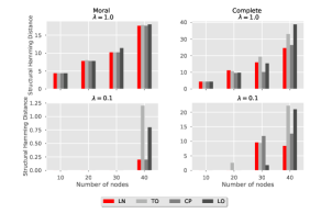
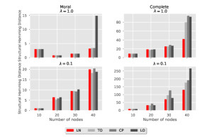
Figures 6(a)-(b) show the SHDs for all formulations for and , respectively. Comparing Figure 6(a) with Figure 6(b), we observe that the SHD tends to increase as the number of samples decreases. As discussed earlier, when , penalized likelihood likelihood estimate with an regularization ensures identifiability in our setting [33, 41]. However, for a finite sample size, identifiability may not be guaranteed. Moreover, the appropriate choice of for may be different than the corresponding for .
Figure 6(a) shows that all methods learn the true DAG with , and given a moral graph for . In addition, SHD is negligible for LN and CP formulations for . However, we observe a substantial increase in SHD (e.g., from 0.2 to near 10 for LN) for complete graphs. These figures indicate the importance of incorporating available structural knowledge (e.g., a moral graph) for better estimation of the true DAG.
While, in general, LN performs well compared with other formulations, we do not expect to see a clear dominance in terms of accuracy of DAG estimation either due to finite samples or the fact that none of the methods could attain a global optimal solution for larger instances. On the contrary, we retrieve the true DAG for smaller graphs for which optimal solutions are obtained. As pointed out in [29], a slight change in the objective function value could significantly alter the estimated DAG. Our results corroborate this observation.

5.3 Comparison of formulations
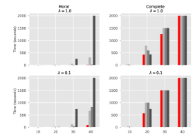
Figure 7 shows various average metrics across 10 random graphs for regularization with samples. Figure 7(a) shows that the LN formulation clearly outperforms other formulations in terms of average optimality gap across all number of nodes, , and regularization parameters, . Moreover, Figure 7(b) shows that the LN formulation requires significantly less computational time in moral instances, and in complete instances with compared to other methods. In complete instances, all methods hit the time limit for . Figures 7(c)-(f) can be interpreted similar to the Figures 5(c)-(f) for regularization. Similar to regularization, Figures 7(a)-(b) demonstrate the importance of incorporating structural knowledge (e.g., a moral graph) for regularization. Similar results are observed for samples; see Appendix II.
As expected, the DAG estimation accuracy with regularization is inferior to the regularization. This is in part due to the bias associated with the regularization, which could be further controlled with, for example, adaptive -norm regularization [47]. Nonetheless, formulations for regularization require less computational time and are easier to solve than the corresponding formulations for regularization.


6 Comparison with the A⋆-lasso algorithm
In this section, we compare the LN formulation with A⋆-lasso [42], using the MATLAB code made available by the authors. For this comparison, the same true DAG structures are taken from [42] and the strength of arcs () are chosen from . The number of nodes in the 10 true DAGs varies from to (see Table 2). The true DAG and resulting random coefficients are used to generate samples for each column of data matrix .
A time limit of six hours is imposed across all experiments after which runs are aborted. In addition, for a fairer comparison with A⋆-lasso, we do not impose an MIQP gap termination criterion of 0.001 for LN and use the Gurobi default optimality gap criterion of 0.0001.
Similar to synthetic data described in Section 5.1, we consider two cases: (i) moral instances and (ii) complete instances. For the former case, the moral graph is constructed from the true DAG as done in Section 5.1. The raw observational data (i.e., ) for moral and complete instances are the same.
We compare the LN formulation with A⋆-lasso using regularization. Note that A⋆-lasso cannot solve the model with regularization. Furthermore, the original A⋆-lasso algorithm assumes no super-structure. Therefore, to enhance its performance, we modified the MATLAB code for A⋆-lasso in order to incorporate the moral graph structure, when available. We consider two values for for our comparison. As decreases, identifying an optimal DAG becomes more difficult. Thus, it is of interest to evaluate the computational performance of both methods for (i.e., no regularization) to assess the performance of these approaches on difficult cases (see, e.g., the computational results in [46] and the statistical analysis in [25] for ). We note that model selection methods (such as Bayesian Information Criterion [38]) can be used to identify the best value of . However, in this section, our focus is to evaluate the computational performance of these approaches for a given value.
Table 2 shows the solution times (in seconds) of A⋆-lasso versus the LN formulation for complete and moral instances. For the LN formulation, if the algorithm cannot prove optimality within the 6-hour time limit, we stop the algorithm and report, in parentheses, the optimality gap at termination. For complete instances with , the results highlight that for small instances (up to 14 nodes) A⋆-algorithm performs better, whereas the LN formulation outperforms A⋆-lasso for larger instances. In particular, we see that the LN formulation attains the optimal solution for the Cloud data set in 810.47 seconds and it obtains a feasible solution that is provably within 99.5% of the optimal objective value for Funnel and Galaxy data sets. For moral instances, we observe significant improvement in the computational performance of the LN formulation, whereas the improvement in A⋆-lasso is marginal in comparison. This observation highlights the fact that dynamic programming-based approaches cannot effectively utilize the super-structure knowledge, whereas an IP-based approach, particularly the LN formulation, can significantly reduce the computational times. For instance, LN’s computational time for the Cloud data reduces from seconds to less than two seconds when the moral graph is provided. In contrast, the reduction in computational time for A⋆-algorithm with the moral graph is negligible. For , the problem is easier to solve. Nevertheless, LN performs well in comparison to A⋆-lasso and the performance of the LN formulation improves for moral instances.
For DAG learning from discrete data, an IP-based model (see e.g., [19]) outperforms A⋆ algorithms when a cardinality constraint on the number of the parent set for each node is imposed; A⋆ tends to perform better if such constraints are not enforced. This is mainly because an IP-based model for discrete data requires an exponential number of variables which becomes cumbersome if such cardinality constraints are not permitted. In contrast, for DAG learning from continuous data with linear SEMs, our results show that an IP-based approach does not have such a limitation because variables are encoded in the space of arcs (instead of parent sets). That is why LN performs well even for complete instances (i.e., no restriction on the cardinality of parent set).
There are several fundamental advantages of IP-based modeling, particularly the LN formulation, compared to A⋆-lasso: (i) The variables in IP-based models (i.e., TO, LN, and CP) depend on the super-structure. Therefore, these IP-based models can effectively utilize the prior knowledge to reduce the search space, whereas A⋆-lasso cannot utilize the super-structure information as effectively. This is particularly important for the LN formulation, as the number of variables and constraints depend only on the super-structure; (ii) all IP-based models can incorporate both and regularizations, whereas A⋆-lasso can solve the problem only with regularization; (iii) all IP-based methods in general enjoy the versatility to incorporate a wide variety of structural constraints, whereas A⋆-lasso and dynamic programming approaches cannot accommodate many structural assumptions. For instance, a modeler may prefer restricting the number of arcs in the DAG, this is achievable by imposing a constraint on an IP-based model, whereas one cannot impose such structural knowledge on A⋆-lasso algorithm; (iv) A⋆-lasso is based on dynamic programming; therefore, one cannot abrupt the search with the aim of achieving a feasible solution. On the other hand, one can impose a time limit or an optimality gap tolerance to stop the search process in a branch-and-bound tree. The output is then a feasible solution to the problem, which provides an upper bound as well as a lower bound which guarantees the quality of the feasible solution; (v) algorithmic advances in integer optimization alone (such as faster continuous relaxation solution, heuristics for better upper bounds, and cutting planes for better lower bounds) have resulted in 29,000 factor speedup in solving IPs [4] using a branch-and-bound process. Many of these advances have been implemented in powerful state-of-the-art optimization solvers (e.g., Gurobi), but they cannot be used in dynamic programming methods, such as A⋆-lasso.
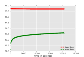
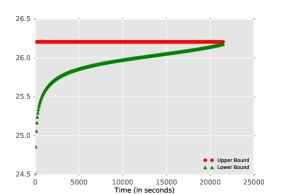
Figures 9(a)-(b) illustrate the progress of upper bound versus lower bound in the branch-and-bound process for the Factor dataset and highlight an important practical implication of an IP-based model: such models often attain high quality upper bounds (i.e., feasible solutions) in a short amount of time whereas the rest of the time is spent to close the optimality gap by increasing the lower bound.
The results for the moral graph in Figure 9(b) highlight another important observation. That is, providing the moral graph can significantly accelerate the progress of the lower bound in the branch-and-bound process. In other words, information from the moral graph helps close the optimality gap more quickly.
| Moral | Complete | Moral | Complete | ||||||||||||
| Graphs (Data sets) | m | A⋆-lasso | LN | A⋆-lasso | LN | A⋆-lasso | LN | A⋆-lasso | LN | ||||||
| dsep | 6 | 16 | 0.017 | 0.378 | 0.0261 | 0.388 | 0.455 | 0.025 | 0.429 | 0.108 | |||||
| Asia | 8 | 40 | 0.016 | 0.401 | 0.152 | 0.887 | 0.195 | 0.071 | 0.191 | 0.319 | |||||
| Bowling | 9 | 36 | 0.018 | 0.554 | 0.467 | 1.31 | 0.417 | 0.225 | 0.489 | 0.291 | |||||
| Insurancesmall | 15 | 76 | 391 | 2.719 | 547.171 | 613.543 | 2.694 | 1.135 | 3.048 | 0.531 | |||||
| Rain | 14 | 70 | 119.15 | 1.752 | 101.33 | 246.25 | 51.737 | 0.632 | 69.404 | 3.502 | |||||
| Cloud | 16 | 58 | 4433.29 | 1.421 | 18839 | 810.471 | 1066.08 | 0.426 | 2230.035 | 7.249 | |||||
| Funnel | 18 | 62 | 6 hrs | 1.291 | 6 hrs | 6 hrs (.002) | 6 hrs | 0.395 | 6 hrs | 3.478 | |||||
| Galaxy | 20 | 76 | 6 hrs | 1.739 | 6 hrs | 6 hrs (.005) | 6 hrs | 0.740 | 6 hrs | 9.615 | |||||
| Insurance | 27 | 168 | 6 hrs | 131.741 | 6 hrs | 6 hrs (.162) | 6 hours | 12.120 | 6 hrs | 6 hrs (.031) | |||||
| Factors | 27 | 310 | 6 hrs | 6 hrs (.001) | 6 hrs | 6 hrs (.081) | 6 hours | 55.961 | 6 hrs | 6 hrs (.01) | |||||
7 Conclusion
In this paper, we study the problem of learning an optimal DAG from continuous observational data using a score function, where the causal effect among the random variables is linear. We cast the problem as a mathematical program and use a penalized negative log-likelihood score function with both and regularizations. The mathematical programming framework can naturally incorporate a wide range of structural assumptions. For instance, it can incorporate a super-structure (e.g., skeleton or moral graph) in the form of an undirected and possibly cyclic graph. Such super-structures can be estimated from observational data. We review three mathematical formulations: cutting plane (CP), topological ordering (TO), and Linear Ordering (LO), and propose a new mixed-integer quadratic optimization (MIQO) formulation, referred to as the layered network (LN) formulation. We establish that the continuous relaxations of all models attain the same optimal objective function value under a mild condition. Nonetheless, the LN formulation is a compact formulation in contrast to CP, its relaxation can be solved much more efficiently compared to LO, and enjoys a fewer number of binary variables and traces a fewer number of branch-and-bound nodes than TO.
Our numerical experiments indicate that these advantages result in considerable improvement in the performance of LN compared to other MIQP formulations (CP, LO, and TO). These improvements are particularly pronounced when a sparse super-structure is available, because LN is the only formulation in which the number of constraints and binary variables solely depend on the super-structure. Our numerical experiments also demonstrate that the LN formulation has a number of advantages over the A⋆-lasso algorithm, especially when a sparse super-structure is available.
At least two future research avenues are worth exploring. First, one of the difficulties of estimating DAGs using mathematical programming techniques is the constraints in (6b). The big- constraint is often very loose, which makes the convergence of branch-and-bound process slow. It is of interest to study these constraints in order to improve the lower bounds obtained from continuous relaxations. Second, in many real-world applications, the underlying DAG has special structures. For instance, the true DAG may be a polytree [12]. Another example is a hierarchical structure. In that case, it is natural to learn a DAG such that it satisfies the hierarchy among different groups of random variables. This problem has important applications in discovering the genetic basis of complex diseases (e.g., asthma, diabetes, atherosclerosis).
References
- [1] Bryon Aragam and Qing Zhou. Concave penalized estimation of sparse Gaussian Bayesian networks. Journal of Machine Learning Research, 16:2273–2328, 2015.
- [2] Mark Bartlett and James Cussens. Advances in Bayesian network learning using integer programming. arXiv preprint arXiv:1309.6825, 2013.
- [3] Mark Bartlett and James Cussens. Integer linear programming for the Bayesian network structure learning problem. Artificial Intelligence, 244:258–271, 2017.
- [4] Dimitris Bertsimas, Angela King, Rahul Mazumder, et al. Best subset selection via a modern optimization lens. The annals of statistics, 44(2):813–852, 2016.
- [5] David Maxwell Chickering. Learning Bayesian networks is NP-complete. In Learning from data, pages 121–130. Springer, 1996.
- [6] David Maxwell Chickering. Optimal structure identification with greedy search. Journal of machine learning research, 3(Nov):507–554, 2002.
- [7] James Cussens. Maximum likelihood pedigree reconstruction using integer programming. In WCB@ ICLP, pages 8–19, 2010.
- [8] James Cussens. Bayesian network learning with cutting planes. arXiv preprint arXiv:1202.3713, 2012.
- [9] James Cussens, David Haws, and Milan Studenỳ. Polyhedral aspects of score equivalence in Bayesian network structure learning. Mathematical Programming, 164(1-2):285–324, 2017.
- [10] James Cussens, Matti Järvisalo, Janne H Korhonen, and Mark Bartlett. Bayesian network structure learning with integer programming: Polytopes, facets and complexity. J. Artif. Intell. Res.(JAIR), 58:185–229, 2017.
- [11] George Dantzig, Ray Fulkerson, and Selmer Johnson. Solution of a large-scale traveling-salesman problem. Journal of the operations research society of America, 2(4):393–410, 1954.
- [12] Sanjoy Dasgupta. Learning polytrees. In Proceedings of the Fifteenth conference on Uncertainty in artificial intelligence, pages 134–141. Morgan Kaufmann Publishers Inc., 1999.
- [13] Daniel Eaton and Kevin Murphy. Exact Bayesian structure learning from uncertain interventions. In Artificial Intelligence and Statistics, pages 107–114, 2007.
- [14] Fei Fu and Qing Zhou. Learning sparse causal Gaussian networks with experimental intervention: regularization and coordinate descent. Journal of the American Statistical Association, 108(501):288–300, 2013.
- [15] Asish Ghoshal and Jean Honorio. Information-theoretic limits of Bayesian network structure learning. In Aarti Singh and Jerry Zhu, editors, Proceedings of the 20th International Conference on Artificial Intelligence and Statistics, volume 54 of Proceedings of Machine Learning Research, pages 767–775, Fort Lauderdale, FL, USA, 20–22 Apr 2017. PMLR.
- [16] Martin Grötschel, Michael Jünger, and Gerhard Reinelt. On the acyclic subgraph polytope. Mathematical Programming, 33(1):28–42, 1985.
- [17] Sung Won Han, Gong Chen, Myun-Seok Cheon, and Hua Zhong. Estimation of directed acyclic graphs through two-stage adaptive lasso for gene network inference. Journal of the American Statistical Association, 111(515):1004–1019, 2016.
- [18] Patrick Healy and Nikola S Nikolov. A branch-and-cut approach to the directed acyclic graph layering problem. In International Symposium on Graph Drawing, pages 98–109. Springer, 2002.
- [19] Tommi Jaakkola, David Sontag, Amir Globerson, and Marina Meila. Learning Bayesian network structure using LP relaxations. In Proceedings of the Thirteenth International Conference on Artificial Intelligence and Statistics, pages 358–365, 2010.
- [20] Markus Kalisch and Peter Bühlmann. Estimating high-dimensional directed acyclic graphs with the PC-algorithm. Journal of Machine Learning Research, 8(Mar):613–636, 2007.
- [21] Mikko Koivisto. Advances in exact Bayesian structure discovery in Bayesian networks. arXiv preprint arXiv:1206.6828, 2012.
- [22] Mikko Koivisto and Kismat Sood. Exact Bayesian structure discovery in Bayesian networks. Journal of Machine Learning Research, 5(May):549–573, 2004.
- [23] Daphne Koller and Nir Friedman. Probabilistic graphical models: principles and techniques. MIT press, 2009.
- [24] Steffen L. Lauritzen. Graphical Models. Oxford University Press, 1996.
- [25] Po-Ling Loh and Peter Bühlmann. High-dimensional learning of linear causal networks via inverse covariance estimation. The Journal of Machine Learning Research, 15(1):3065–3105, 2014.
- [26] Brandon Malone, Kustaa Kangas, Matti Järvisalo, Mikko Koivisto, and Petri Myllymäki. Predicting the hardness of learning Bayesian networks. In AAAI, pages 2460–2466, 2014.
- [27] Florian Markowetz and Rainer Spang. Inferring cellular networks–a review. BMC bioinformatics, 8(6):S5, 2007.
- [28] George L Nemhauser and Laurence A Wolsey. Integer programming and combinatorial optimization. Wiley, Chichester. GL Nemhauser, MWP Savelsbergh, GS Sigismondi (1992). Constraint Classification for Mixed Integer Programming Formulations. COAL Bulletin, 20:8–12, 1988.
- [29] Young Woong Park and Diego Klabjan. Bayesian network learning via topological order. The Journal of Machine Learning Research, 18(1):3451–3482, 2017.
- [30] Pekka Parviainen and Mikko Koivisto. Exact structure discovery in Bayesian networks with less space. In Proceedings of the Twenty-Fifth Conference on Uncertainty in Artificial Intelligence, pages 436–443. AUAI Press, 2009.
- [31] Judea Pearl et al. Causal inference in statistics: An overview. Statistics surveys, 3:96–146, 2009.
- [32] Eric Perrier, Seiya Imoto, and Satoru Miyano. Finding optimal Bayesian network given a super-structure. Journal of Machine Learning Research, 9(Oct):2251–2286, 2008.
- [33] Jonas Peters and Peter Bühlmann. Identifiability of Gaussian structural equation models with equal error variances. Biometrika, 101(1):219–228, 2013.
- [34] Garvesh Raskutti and Caroline Uhler. Learning directed acyclic graphs based on sparsest permutations. arXiv preprint arXiv:1307.0366, 2013.
- [35] Ali Shojaie and George Michailidis. Penalized likelihood methods for estimation of sparse high-dimensional directed acyclic graphs. Biometrika, 97(3):519–538, 2010.
- [36] Tomi Silander and Petri Myllymaki. A simple approach for finding the globally optimal Bayesian network structure. arXiv preprint arXiv:1206.6875, 2012.
- [37] Liam Solus, Yuhao Wang, Lenka Matejovicova, and Caroline Uhler. Consistency guarantees for permutation-based causal inference algorithms. arXiv preprint arXiv:1702.03530, 2017.
- [38] A Sondhi and A Shojaei. The reduced PC-algorithm: Improved causal structure learning in large random networks. arXiv preprint arXiv:1806.06209, 2018.
- [39] Peter Spirtes, Clark N Glymour, and Richard Scheines. Causation, prediction, and search. MIT press, 2000.
- [40] Robert Tibshirani. Regression shrinkage and selection via the lasso. Journal of the Royal Statistical Society. Series B (Methodological), pages 267–288, 1996.
- [41] Sara van de Geer and Peter Bühlmann. -penalized maximum likelihood for sparse directed acyclic graphs. The Annals of Statistics, 41(2):536–567, 2013.
- [42] Jing Xiang and Seyoung Kim. A* lasso for learning a sparse Bayesian network structure for continuous variables. In Advances in neural information processing systems, pages 2418–2426, 2013.
- [43] Changhe Yuan and Brandon Malone. Learning optimal Bayesian networks: A shortest path perspective. Journal of Artificial Intelligence Research, 48:23–65, 2013.
- [44] Changhe Yuan, Brandon Malone, and Xiaojian Wu. Learning optimal Bayesian networks using A* search. In IJCAI proceedings-international joint conference on artificial intelligence, volume 22, page 2186, 2011.
- [45] Bin Zhang, Chris Gaiteri, Liviu-Gabriel Bodea, Zhi Wang, Joshua McElwee, Alexei A Podtelezhnikov, Chunsheng Zhang, Tao Xie, Linh Tran, Radu Dobrin, et al. Integrated systems approach identifies genetic nodes and networks in late-onset Alzheimer’s disease. Cell, 153(3):707–720, 2013.
- [46] Xun Zheng, Bryon Aragam, Pradeep Ravikumar, and Eric P Xing. DAGs with NO TEARS: smooth optimization for structure learning. arXiv preprint arXiv:1803.01422, 2018.
- [47] Hui Zou. The adaptive lasso and its oracle properties. Journal of the American statistical association, 101(476):1418–1429, 2006.
Appendix I
PROOF OF PROPOSITION 1
Let be an optimal solution for (5) with an optimal objective value . Let us refer to the DAG structure corresponding to this optimal solution by . Suppose that for some , we have . To prove the proposition, we construct an optimal solution which satisfies for all pairs of and meets the following conditions: (i) this corresponding DAG (tournament) is cycle free (ii) this tournament has the same objective value, i.e., , as an optimal DAG.
Select a pair of nodes, say from for which . If there is a directed path from to (respectively to ), then we can add the following arc (respectively, ). This arc does not create a cycle in the graph. If there is no directed path between and , we can add an arc in either direction. In all cases, set value corresponding to the added arc to zero. We repeat this process for all pairs of nodes with .
We can add such arcs without creating any cycle. This is because if we cannot add an arc in either direction, it implies that we should have a directed path from to and a directed path from to in graph which is a contradiction because it implies a directed cycle in an optimal DAG. Note that in each step, we maintain a DAG. Hence, by induction we conclude that condition (i) is satisfied. The pair of nodes can be chosen arbitrarily.
Since in the constructed solution we set for the added arcs as zero, the objective value does not change. This satisfies condition (ii), and completes the proof.
PROOF OF PROPOSITION 2
First we prove that (10e) removes all cycles. Suppose, for contradiction, that a cycle of size is available and represented by . This implies , and . Then,
We sum the above inequalities and conclude , a contradiction.
To complete the proof, we also need to prove that any DAG is feasible for the LN formulation. To this end, we know that each DAG has a topological ordering. For all the existing arcs in the DAG, substitute and assign a topological ordering number to the variables in LN. Then, the set of constraints in (10e) is always satisfied.
PROOF OF PROPOSITION 3
The LO formulation is in -space whereas LN is in -space. Hence, we first construct a mapping between these decision variables.
Given a feasible solution for all in the LO formulation, we define , and , . Let be a function which takes value 1 if and 0 otherwise. Given for all and for in the LN formulation, we map for all and for all . Note that -space is defined for all pair of nodes whereas -space is defined for the set of arcs in . In every correct mapping, we have .
Fixing and for each and summing the left hand-side of inequalities (8e) over we obtain
where the equivalences follow from constraints (8d). Given our mapping, for all and for , the above set of constraints can be written as
which satisfies (10e) in the LN formulation. This implies for -regularization. For -regularization, we need to add that . This implies for regularization.
To show strict containment, we give a point that is feasible to the LN formulation that cannot be mapped to any feasible point in the LO formulation. Consider , , , for , with an appropriate choice of . It is easy to check that this is a feasible solution to the LN formulation. Because we must have , we have . Therefore, the corresponding point is infeasible to the LO formulation and this completes the proof.
PROOF OF PROPOSITION 4
This proof is for TO formulation when the parameter on (9e) is replaced with .
In the TO formulation, define the term as and the term as . Further, remove the set of constraints in (9f), (9g), and (9i). This implies that . To see strict containment, consider the point described in the proof of Proposition 3, which is feasible to the LN formulation. For this point, there can be no feasible assignment of the decision matrix such that , hence .
PROOF OF PROPOSITION 5
Let denote the optimal objective value associated with the continuous relaxation of model .
Part A. .
Case 1. regularization
Suppose () is an optimal solution associated with the continuous relaxation of the LN formulation (10a)-(10g) and () is an optimal solution associated with continuous relaxation of the LO formulation with -regularization.
Given Proposition 3, we conclude that . We prove that also holds in an optimal solution. To this end, we map an optimal solution in continuous relaxation of the -LN formulation to a feasible solution in continuous relaxation of the -LO formulation with the same objective function. This implies .
Given an optimal solution () to the continuous relaxation of the -LN formulation, we construct a feasible solution to the continuous relaxation of the LO formulation as
and let .
We now show that this mapping is always valid for the -LO formulation. Recall that for the regularization, we do not have the decision vector in the formulation. Three set of constraints have to be satisfied in the -LO formulation.
The set of constraints (8b) is trivially satisfied because we set . The set of constraints (8d) is trivially satisfied. The set of constraints (8e) is satisfied because the left hand side of inequality can take at most given this mapping. Therefore, . This completes this part of the proof.
Case 2. regularization
Suppose () is an optimal solution associated with a continuous relaxation of the -LN formulation, and () is an optimal solution associated with a continuous relaxation of the -LO formulation.
Given Proposition 3, . We now prove that, in an optimal solution also holds.
Given an optimal solution () for the continuous relaxation of the -LN formulation, we construct a feasible solution for the continuous relaxation of the -LO formulation as
and let and .
We now show that this mapping is always valid for the LO formulation. Four sets of constraints have to be satisfied in the LO formulation.
The set of constraints in (8d) is satisfied similar to case. The proof that constraints (8b), (8c), and (8e) are also met is more involved. If the -LN formulation attains a solution for which (we dropped subscript LN), then our mapping leads to an infeasible solution to the -LO formulation, because it forces for -LO. Next we show that this will not be the case and that our mapping is valid. To this end, we show that in an optimal solution for the continuous relaxation of -LN, we always have . Note that in the LN formulation, we have and (we dropped the subscript LN). Suppose that . In this case, the objective function forces to be at most . Note that the objective function can reduce up to and decreases the regularization term without any increase on the loss function. This is because can be replaced by without any restriction on because . Therefore, our mapping is valid and implies that .
Part B. .
Case 1. regularization
Given Proposition 4, we conclude that . We now prove that also holds in an optimal solution. We map an optimal solution in continuous relaxation of the -LN formulation to a feasible solution in continuous relaxation of the -TO formulation with the same objective value. This implies .
Next we construct a feasible solution to the TO formulation. Given an optimal solution (, ) for a continuous relaxation of the LN formulation, rank the in non-descending order. Ties between values can be broken arbitrarily in this ranking. Then, for each variable , where denotes the rank of in a non-descending order (the first element is ranked 0). This mapping satisfies the two assignment constraints (9f)-(9g). Let , . This gives a feasible solution for the TO formulation. Thus,
Case 2. regularization
Define . The rest of the proof is similar to the previous proofs.
Part C. .
To prove this, we first prove the following Lemma.
Lemma. The LO formulation is at least as strong as the CP formulation, that is .
Consider the set of constraints in CP given by (6c) as
Consider the same mapping as in Proposition 3. Select an arbitrary constraint from (6c). Without loss of generality, consider . We arrange the terms in (8d)-(8e) as
Summing the above set of inequalities and substituting , when appropriate, gives . Thus, we conclude that .
Given this lemma and Proposition 3, we conclude that .
PROOF OF PROPOSITION 6
This is a generalization of Proposition 5. Suppose we have branched on variable in the LO formulation or correspondingly on variable in the LN formulation. If , then . In this case, it is as if we now need to solve the original model with . Thus, Proposition 5 (Part A) implies that both models attain the same continuous relaxation. On the other hand, if in LO (or correspondingly in LN), we define our mapping as
where is the set of for which . The rest of the proof follows from Proposition 5 (Part A).
The proofs for the TO and CP formulations are almost identical with Proposition 5. Suppose we have branched on variable on any of the models (CP, LO, TO). If , then . In this case, it is as if we now need to solve the original model with . If , one defines the mapping in Proposition 5. The proof follows from Proposition 5 parts B and C, respectively.
Appendix II