Fractional Calculus in Pharmacokinetics

Abstract

We are witnessing the birth of a new variety of pharmacokinetics where non-integer-order differential equations are employed to study the time course of drugs in the body: this is dubbed “fractional pharmacokinetics”. The presence of fractional kinetics has important clinical implications such as the lack of a half-life, observed, for example with the drug amiodarone and the associated irregular accumulation patterns following constant and multiple-dose administration. Building models that accurately reflect this behaviour is essential for the design of less toxic and more effective drug administration protocols and devices. This article introduces the readers to the theory of fractional pharmacokinetics and the research challenges that arise. After a short introduction to the concepts of fractional calculus, and the main applications that have appeared in literature up to date, we address two important aspects. First, numerical methods that allow us to simulate fractional order systems accurately and second, optimal control methodologies that can be used to design dosing regimens to individuals and populations.

Introduction

Background

Diffusion is one of the main mechanisms of various transport processes in living species and plays an important role in the distribution of drugs in the body. Processes such as membrane permeation, dissolution of solids and dispersion in cellular matrices are considered to take place by diffusion. Diffusion is typically described by Fick’s law, which, in terms of the pharmacokinetics of drugs, gives rise to exponential washout curves that have a characteristic time scale, usually expressed as a half-life. However, in the last few decades, strong experimental evidence has suggested that this is not always true and diffusion processes that deviate from this law have been observed. These are either faster (super-diffusion) or slower (sub-diffusion) modes of diffusion compared to the regular case West and Deering (1994); Ionescu et al (2017).

Such types of diffusion give rise to kinetics that are referred to as anomalous to indicate the fact that they stray from the standard diffusion dynamics West and Deering (1994). Moreover, anomalous kinetics can also result from reaction-limited processes and long-time trapping. Anomalous kinetics introduces memory effects into the distribution process that need to be accounted for to correctly describe it. An distinctive feature of anomalous power-law kinetics is that it lacks a characteristic time scale contrary to exponential kinetics. A mathematical formulation that describes such anomalous kinetics is known as fractal kinetics Kopelman (1988); Macheras (1996); Pereira (2010) where explicit power functions of time in the form of time-dependent coefficients are used to account for the memory effects replacing the original rate constants. In pharmacokinetics several datasets have been characterised by power laws, epmpirically Wise (1985); Tucker et al (1984), while the first article that utilised fractal kinetics in pharmacokinetics was Macheras (1996). Molecules that their kinetics presents power law behaviour incude those distributed in deeper tissues, such as amiodarone Weiss (1999) and bone-seeking elements, such as calcium, lead, strontium and plutonium Macheras (1996); Phan et al (2006).

An alternative theory to describe anomalous kinetics employs fractional calculus Sokolov et al (2002); Podlubny (1999), which introduces derivatives and integrals of fractional order, such as half or three quarters. Although fractional calculus was introduced by Leibniz more than 300 years ago, it is only within the last couple of decades that real-life applications have been explored Magin (2004a, b, c). It has been shown that differential equations with fractional derivatives (FDEs) describe experimental data of anomalous diffusion more accurately. Although fractional-order derivatives were first introduced as a novel mathematical concept with unclear physical meaning, nowadays, a clear connection between diffusion over fractal spaces (such as networks of capillaries) and fractional-order dynamics has been established Butera and Paola (2014); Chen et al (2010); Metzler et al (1994); Copot et al (2014). In particular, in anomalous diffusion the standard assumption that the mean square displacement $\langle x^{2}\rangle$ is proportional to time does not hold. Instead, it is $\langle x^{2}\rangle\sim t^{\nicefrac{{2}}{{d}}}$, where $d\neq 2$ is the associated fractal dimension Gmachowski (2015); Klafter and Sokolov (2011); Eirich (1990).

Fractional kinetics Dokoumetzidis and Macheras (2011) was introduced in the pharmaceutical literature in Dokoumetzidis and Macheras (2009) and the first example of fractional pharmacokinetics which appeared in that article was amiodarone, a drug known for its power-law kinetics Tucker et al (1984). Since then, other applications of fractional pharmacokinetics have appeared in the literature. Kytariolos et al. Kytariolos et al (2010) presented an application of fractional kinetics for the development of nonlinear in vitro-in vivo correlations. Popović et al. have presented several applications of fractional pharmacokinetics to model drugs, namely for diclofenac Popović et al (2010), valproic acid Popović et al (2011), bumetanide Popović et al (2013) and methotrexate Popović et al (2015). Copot et al. have further used a fractional pharmacokinetics model for propofol Copot et al (2013). In most of these cases the fractional model has been compared with an equivalent ordinary PK model and was found superior. FDEs have been proposed to describe drug response too, apart from their kinetics. Verotta has proposed several alternative fractional PKPD models that are capable of describing pharmacodynamic times series with favourable properties Verotta (2010). Although these models are empirical, i.e., they have no mechanistic basis, they are attractive since the memory effects of FDEs can link smoothly the concentration to the response with a variable degree of influence, while the shape of the responses generated by fractional PKPD models can be very flexible and parsimonious (modelled using few parameters).

Applications of FDEs in pharmacokinetics fall in the scope of the newly-coined discipline of mathematical pharmacology Van der Graaf et al (2015) to which this issue is dedicated. Mathematical pharmacology utilises applied mathematics, beyond the standard tools used commonly in pharmacometrics, to describe drug processes in the body and assist in controlling them.

This paper introduces the basic principles of fractional calculus and FDEs, reviews recent applications of fractional calculus in pharmacokinetics and discusses their clinical implications. Moreover, some aspects of drug dosage regimen optimisation based on control theory are presented for the case of pharmacokinetic models that follow fractional kinetics. Indeed, in clinical pharmacokinetics and therapeutic drug monitoring, dose optimisation is carried out usually by utilising Bayesian methodology. Optimal control theory is a powerful approach that can be used to optimise drug administration, which can handle complicated constraints and has not been used extensively for this task. The case of fractional pharmacokinetic models is of particular interest for control theory and poses new challenges.

A problem that has hindered the applications of fractional calculus is the lack of efficient general-purpose numerical solvers, as opposed to ordinary differential equations. However, in the past few years significant progress has been achieved in this area. This important issue is discussed in the paper and some techniques for numerical solution of FDEs are presented.

Fractional derivatives

Derivatives of integer order $n\in\mathbb{N}$, of functions $f:\mathbb{R}\to\mathbb{R}$ are well defined and their properties have been extensively studied in real analysis. The basis for the extension of such derivatives to real orders $\alpha\in\mathbb{R}$ commences with the definition of an integral of order $\alpha$ which hinges on Cauchy’s iterated ($n$-th order) integral formula and gives rise to the celebrated Riemann-Liouville integral ${{}_{0}^{\mathrm{rl}}\mathrm{I}}^{\alpha}_{t}$ Hennion and Hanert (2013):

$${{}_{0}^{\mathrm{rl}}\mathrm{I}}^{\alpha}_{t}f(t)={}_{0}\mathrm{D}_{t}^{-\alpha}f(t)=\tfrac{1}{\Gamma(\alpha)}\int_{0}^{t}(t-\tau)^{\alpha-1}f(\tau)\mathrm{d}\tau,$$ (1)

where $\Gamma$ is the Euler gamma function. In Eq. (1) we assume that $f$ is such that the involved integral is well-defined and finite. This is the case if $f$ is continuous everywhere except at finitely many points and left-bounded, i.e., $\{f(x);0\leq x\leq t\}$ is bounded for every $t\geq 0$. Note that for $\alpha\in\mathbb{N}$, ${{}_{0}^{\mathrm{rl}}\mathrm{I}}^{\alpha}_{t}f$ is equivalent to the ordinary $\alpha$-th order integral. Hereafter, we focus on derivatives of order $\alpha\in[0,1]$ as only these are of interest to date in the study of fractional pharmacokinetics.

The left-side subscript $0$ of the ${}_{0}\mathrm{D}_{t}^{\alpha}$ and ${{}_{0}^{\mathrm{rl}}\mathrm{I}}_{t}^{\alpha}$ operators, denotes the lower end of the integration limits, which in this case has been assumed to be zero. However, alternative lower bounds can be considered leading to different definitions of the fractional derivative with slightly different properties. When the lower bound is $-\infty$, the entire history of the studied function is accounted for, which is considered preferable in some applications and is referred to as the Weyl definition Magin (2004a).

It is intuitive to define a fractional-order derivative of order $\alpha$ via ${}_{0}\mathrm{D}_{t}^{\alpha}=\mathrm{D}^{1}{\,}_{0}\mathrm{D}_{t}^{\alpha-1}=\mathrm{D}^{1}\,{{}_{0}^{\mathrm{rl}}\mathrm{I}}^{\alpha-1}$, (where $\mathrm{D}^{1}$ is the ordinary derivative of order $1$), or equivalently

$${}_{0}\mathrm{D}_{t}^{\alpha}f(t)=\tfrac{\mathrm{d}}{\mathrm{d}t}\left[\tfrac{1}{\Gamma(1-\alpha)}\int_{0}^{t}\frac{f(\tau)}{(t-\tau)^{\alpha}}\mathrm{d}\tau\right]$$ (2)

This is the Riemann-Liouville definition — one of the most popular constructs in fractional calculus. One may observe that the fractional integration is basically a convolution between function $f$ and a power law of time, i.e., ${}_{0}\mathrm{D}_{t}^{-\alpha}f(t)=t^{\alpha-1}\ast f(t)$, where $\ast$ denotes the convolution of two functions. This explicitly demonstrates the memory effects of the studied process. Fractional derivatives possess properties that are not straightforward or intuitive; for example, the half derivative of a constant $f(t)=\lambda$ with respect to $t$ does not vanish and instead is ${}_{0}\mathrm{D}_{t}^{\nicefrac{{1}}{{2}}}\lambda=\nicefrac{{\lambda}}{{\sqrt{\pi t}}}$.

Perhaps the most notable shortcoming of the Riemann-Liouville definition with the $0$ lower bound is that when used in differential equations it gives rise to initial conditions that involve the fractional integral of the function and are difficult to interpret physically. This is one of the reasons the Weyl definition was introduced, but this definition may not be very practical for most applications either, as it involves an initial condition at time $-\infty$ Magin (2004a); Samko et al (1993).

A third definition of the fractional derivative, which is referred to as the Caputo definition is preferable for most physical processes as it involves explicitly the initial condition at time zero. The definition is:

$${}_{0}^{\mathrm{c}}\mathrm{D}_{t}^{\alpha}f(t)=\tfrac{1}{\Gamma(1-\alpha)}\int_{0}^{t}\frac{\tfrac{\mathrm{d}f(\tau)}{\mathrm{d}\tau}}{(t-\tau)^{\alpha}}\mathrm{d}\tau$$ (3)

where the upper-left superscript $\mathrm{c}$ stands for Caputo. The Caputo derivative is interpreted as ${}_{0}^{\mathrm{c}}\mathrm{D}_{t}^{\alpha}={{}_{0}^{\mathrm{rl}}\mathrm{I}}^{\alpha-1}\mathrm{D}^{1}$, that is $\mathrm{D}^{1}$ and ${{}_{0}^{\mathrm{rl}}\mathrm{I}}^{\alpha-1}$ are composed in the opposite way compared to the Riemann-Liouville definition. The Caputo derivative gives rise to initial value problems of the form

$${}_{0}^{\mathrm{c}}\mathrm{D}_{t}^{\alpha}x(t) =F(x(t)),$$ (4a)

$$x(0) =x_{0}.$$ (4b)

This definition for the fractional derivative, apart from the more familiar initial conditions, comes with some properties similar to those of integer-order derivatives, one of them being that the Caputo derivative of a constant is in fact zero. Well-posedeness conditions, for the existence and uniqueness of solutions, for such fractional-order initial value problems are akin to those of integer-order problems Deng and Deng (2014),(Podlubny, 1999, Chap. 3). The various definitions of the fractional derivative give different results, but these are not contradictory since they apply for different conditions and it is a matter of choosing the appropriate one for each specific application. All definitions collapse to the usual derivative for integer values of the order of differentiation.

A fourth fractional derivative definition, which is of particular interest is the Grünwald-Letnikov, which allows the approximate discretisation of fractional differential equations. The Grünwald-Letnikov derivative, similar to integer order derivatives, is defined via a limit of a fractional-order difference. Let us first define the Grünwald-Letnikov difference of order $\alpha$ and step-size $h$ of a left-bounded function $f$ as

$${{}^{\mathrm{gl}}\Delta}^{\alpha}_{h}f(t)=\tfrac{1}{h^{\alpha}}\sum_{j=0}^{\left\lfloor\nicefrac{{t}}{{h}}\right\rfloor}c_{j}^{\alpha}f(t-jh),$$ (5)

with $c^{\alpha}0=1$ and for $j\in\mathbb{N}_{>0}$

$$c_{j}^{\alpha}=(-1)^{j}\prod_{i=0}^{j-1}\frac{\alpha-i}{i+1}.$$ (6)

The Grünwald-Letnikov difference operator leads to the definition of the Grünwald-Letnikov derivative of order $\alpha$ which is defined as (Samko et al, 1993, Section 20)

$${{}^{\mathrm{gl}}\mathrm{D}}_{t}^{\alpha}f(t)=\lim_{h\to 0^{+}}{{}^{\mathrm{gl}}\Delta}^{\alpha}_{h}f(t),$$ (7)

insofar as the limit exists. This definition is of great importance in practice, as it allows us to replace ${{}^{\mathrm{gl}}\mathrm{D}}_{t}$ with ${{}^{\mathrm{gl}}\Delta}_{h}^{\alpha}$ provided that $h$ is adequately small, therefore it serves as an Euler-type discretisation of fractional-order continuous time dynamics. By doing so, we produce a discrete-time yet infinite-dimensional approximation of the system since ${{}^{\mathrm{gl}}\Delta}_{h}^{\alpha}f(t)$ depends on $f(t-jh)$ for all $j\in\mathbb{N}_{>0}$. However, we may truncate this series up to a finite history $\nu$, defining

$${{}^{\mathrm{gl}}\Delta}_{h,\nu}^{\alpha}f(t)=\tfrac{1}{h^{\alpha}}\sum_{j=0}^{\min\{\nu,\left\lfloor\nicefrac{{t}}{{h}}\right\rfloor\}}c_{j}^{\alpha}f(t-jh).$$ (8)

This leads to discrete-time finite-memory approximations which are particularly useful as we shall discuss in what follows.

Fractional Kinetics

The most common type of kinetics encountered in pharmaceutical literature are the so called “zero order” and “first order”. Here the “order” refers to the order of linearity and is not to be confused with the order of differentiation, i.e., a zero order process refers to a constant rate and a first order to a proportional rate. The fractional versions of these types of kinetics are presented below and take the form of fractional-order ordinary differential equations. Throughout this presentation the Caputo version of the fractional derivative is considered for reasons already explained.

Zero-order kinetics

The simplest kinetic model is the zero-order model where it is assumed that the rate of change of the quantity $q$, expressed in [mass] units, is constant and equal to $k_{0}$, expressed in [mass]/[time] units. Zero-order systems are governed by differential equations of the form

$$\frac{\mathrm{d}q}{\mathrm{d}t}=k_{0}.$$ (9)

The solution of this equation with initial condition $q(0)=0$ is

$$q(t)=k_{0}t.$$ (10)

The fractional-order counterpart of such zero-order kinetics can be obtained by replacing the derivative of order $1$ by a derivative of fractional order $\alpha$, that is

$${}_{0}^{\mathrm{c}}\mathrm{D}_{t}^{\alpha}q(t)=k_{0,f},$$ (11)

where $k_{0,f}$ is a constant with units [mass]/[time]^α. The solution of this equation for initial condition $q(0)=0$ is a power law for $t>0$ Podlubny (1999)

$$q(t)=\frac{k_{0,f}}{\Gamma(\alpha+1)}t^{\alpha}.$$ (12)

First-order kinetics

The first-order differential equation, where the rate of change of the quantity $q$ is proportional to its current value, is described by the ordinary differential equation

$$\frac{\mathrm{d}q}{\mathrm{d}t}=-k_{1}q(t).$$ (13)

Its solution with initial condition of $q(0)=q_{0}$ is given by the classical equation of exponential decay

$$q(t)=q_{0}\exp(-k_{1}t).$$ (14)

Likewise, the fractional-order analogue of such first-order kinetics is derived by replacing $\nicefrac{{\mathrm{d}}}{{\mathrm{d}t}}$ by the fractional-order derivative ${}_{0}^{\mathrm{c}}\mathrm{D}_{t}^{\alpha}$ yielding the following fractional differential equation

$${}_{0}^{\mathrm{c}}\mathrm{D}_{t}^{\alpha}q(t)=-k_{1,f}q(t),$$ (15)

where $k_{1,f}$ is a constant with [time]^-α units. The solution of this equation can be found in most books or papers of the fast growing literature on fractional calculus Podlubny (1999) and for initial condition $q(0)=q_{0}$ it is

$$q(t)=q_{0}\mathcal{E}_{\alpha}(-k_{1,f}t^{\alpha}),$$ (16)

where $\mathcal{E}_{\alpha}$ is the Mittag-Leffler function Podlubny (1999) which is defined as

$$\mathcal{E}_{\alpha}(t)=\sum_{k=0}^{\infty}\frac{t^{k}}{\Gamma(\alpha k+1)}.$$ (17)

The function $\mathcal{E}_{\alpha}(t)$ is a generalisation of the exponential function and it collapses to the exponential when $\alpha=1$, i.e., $\mathcal{E}_{1}(t)=\exp(t)$. Alternatively, Eq. (16) can be reparametrised by introducing a time scale parameter with regular time units, $\tau_{f}=k_{1,f}^{-1/\alpha}$ and then becomes $q(t)=q_{0}\mathcal{E}_{\alpha}(-(t/\tau_{f})^{\alpha})$. The solution of Eq. (15) basically means that the fractional derivative of order $\alpha$ of the function $\mathcal{E}_{\alpha}(t^{\alpha})$ is itself a function of the same form, exactly like the classic derivative of an exponential is also an exponential.

It also makes sense to restrict $\alpha$ to values $0\leq\alpha\leq 1$, since for values of a larger than $1$ the solution of Eq. (15) is not monotonic and negative values for $q$ may appear, therefore, it is not applicable in pharmacokinetics and pharmacodynamics. Based on these elementary equations the basic relations for the time evolution in drug disposition can be formulated, with the assumption of diffusion of drug molecules taking place in heterogeneous space. The simplest fractional pharmacokinetic model is the one-compartment model with i.v. bolus administration and the concentration, c, can be expressed by Eq. (16) divided by a volume of distribution, as

$$c(t)=c_{0}\mathcal{E}_{\alpha}(-k_{1,f}t^{\alpha}),$$ (18)

with $\alpha\leq 1$ and $c_{0}$ is the ratio [dose]/[apparent volume of distribution]. This equation for times $t\ll 1$ behaves as a stretched exponential, i.e., as ${\sim}\exp(-k_{1,f}t^{\alpha}/\Gamma(1+\alpha))$, while for large values of time it behaves as a power-law, ${\sim}t^{-\alpha}/\Gamma(1-\alpha)$ (see Figure 1) Mainardi (2014). This kinetics is, therefore, a good candidate to describe various datasets exhibiting power-law-like kinetics due to the slow diffusion of the drug in deeper tissues. Moreover, the relevance of the stretched exponential (Weibull) function with the Mittag-Leffler function probably explains the successful application of the former function in describing drug release in heterogeneous media Papadopoulou et al (2006). Eq. (18) is a relationship for the simplest case of fractional pharmacokinetics. It accounts for the anomalous diffusion process, which may be considered to be the limiting step of the entire kinetics. Classic clearance may be considered not to be the limiting process here and is absent from the equation.

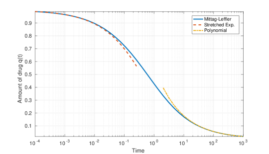
Figure 1: Amount-time profile according to Eq. (16) for $\alpha=0.5$ (solid curve) along with its approximation at values of $t$ close to $0$ by a stretched exponential function $\exp(-t^{\nicefrac{{1}}{{2}}}/\Gamma(1.5))$ (bottom dashed curve) and an approximation at high values of $t$ by a power function $t^{-\nicefrac{{1}}{{2}}}/\Gamma(0.5)$ (top dashed-dotted curve). Note that the time axis is logarithmic. The evolution of the amount of drug starts as a stretched exponential and eventually shapes as a power function.

The Laplace transform for FDEs

Fractional differential equations (FDEs) can be easily written in the Laplace domain since each of the fractional derivatives can be transformed similarly to the ordinary derivatives, as follows, for order $\alpha\leq 1$:

$$\mathcal{L}\{{}_{0}^{\mathrm{c}}\mathrm{D}_{t}^{\alpha}f(t)\}=s^{\alpha}F(s)-s^{\alpha-1}f(0^{+}),$$ (19)

where $F(s)$ is the Laplace transform of $f(t)$ Podlubny (1999). For $\alpha=1$, Eq. (19) reduces to the classic well-known expression for ordinary derivatives, that is, $\mathcal{L}\{\dot{f}(t)\}=sF(s)-f(0^{+})$.

Let us take as an example the following simple FDE

$${}_{0}^{\mathrm{c}}\mathrm{D}_{t}^{1/2}q(t)=-q(t),$$ (20)

with initial value $q(0)=1$ which can be written in the Laplace domain, by virtue of Eq. (19), as follows

$$s^{\nicefrac{{1}}{{2}}}Q(s)-s^{-\nicefrac{{1}}{{2}}}q(0)=-Q(s),$$ (21)

where $Q(s)=\mathcal{L}\{q(t)\}(s)$ is the Laplace transform of $q$. After simple algebraic manipulations, we obtain

$$Q(s)=\frac{1}{s+\sqrt{s}}.$$ (22)

By applying the inverse Laplace transform to Eq. (22) the closed-form analytical solution of this FDE can be obtained; this involves a Mittag-Leffler function of order one half. In particular,

$$q(t)=\mathcal{E}_{\nicefrac{{1}}{{2}}}(-t^{\nicefrac{{1}}{{2}}})=e^{t}(1+\operatorname{erf}(-\sqrt{t})).$$ (23)

Although more often than not it is easy to transform an FDE in the Laplace domain, it is more difficult to apply the inverse Laplace transform so as to solve it explicitly for the system variables so that an analytical solution in the time domain is obtained. However, it is possible to perform that step numerically using a numerical inverse Laplace transform (NILT) algorithm De Hoog et al (1982) as described above.

Fractional Pharmacokinetics

Multi-compartmental models

A one-compartment pharmacokinetic model with i.v. bolus administration can be easily fractionalised as in Eq. (15) by changing the derivative on the left-hand-side of the single ODE to a fractional order. However, in pharmacokinetics and other fields where compartmental models are used, two or more ODEs are often necessary and it is not as straightforward to fractionalise systems of differential equations, especially when certain properties such as mass balance need to be preserved.

When a compartmental model with two or more compartments is built, typically an outgoing mass flux becomes an incoming flux to the next compartment. Thus, an outgoing mass flux that is defined as a rate of fractional order, cannot appear as an incoming flux into another compartment, with a different fractional order, without violating mass balance Dokoumetzidis et al (2010a). It is therefore, in general, impossible to fractionalise multi-compartmental systems simply by changing the order of the derivatives on the left hand side of the ODEs.

One approach to the fractionalisation of multi-compartment models is to consider a common fractional order that defined the mass transfer from a compartment $i$ to a compartment $j$: the outflow of one compartment becomes an inflow to the other. This implies a common fractional order known as a commensurate order. In the general case, of non-commensurate-order systems, a different approach for fractionalising systems of ODEs needs to be applied.

In what follows, a general form of a fractional two-compartment system is considered and then generalised to a system of an arbitrary number of compartments, which first appeared in Dokoumetzidis et al (2010b). A general ordinary linear two-compartment model, is defined by the following system of linear ODEs,

$$\frac{\mathrm{d}q_{1}(t)}{\mathrm{d}t} =-k_{12}q_{1}(t)+k_{21}q_{2}(t)-k_{10}q_{1}(t)+u_{1}(t),$$ (24a)

$$\frac{\mathrm{d}q_{2}(t)}{\mathrm{d}t} =k_{12}q_{1}(t)-k_{21}q_{2}(t)-k_{20}q_{2}(t)+u_{2}(t),$$ (24b)

where $q_{1}(t)$ and $q_{2}(t)$ are the mass or molar amounts of material in the respective compartments and the $k_{ij}$ constants control the mass transfer between the two compartments and elimination from each of them. The notation convention used for the indices of the rate constants is that the first corresponds to the source compartment and the second to the target one, e.g. $k_{12}$ corresponds to the transfer from compartment 1 to 2, $k_{10}$ corresponds to the elimination from compartment 1, etc. The units of all the $k_{ij}$ rate constants are (1/[time]). $u_{i}(t)$ are input rates in each compartment which may be zero, constant or time dependent. Initial values for $q_{1}$ and $q_{2}$ have to be considered also, $q_{1}(0)$ and $q_{2}(0)$, respectively.

In order to fractionalise this system, first the ordinary system is integrated, obtaining a system of integral equations and then the integrals are fractionalised as shown in Dokoumetzidis et al (2010b). Finally, the fractional integral equations, are differentiated in an ordinary way. The resulting fractional system contains ordinary derivatives on the left hand side and fractional Riemann-Liouville derivatives on the right hand side:

$$\frac{\mathrm{d}q_{1}(t)}{\mathrm{d}t} =-k_{12,f}{\,}_{0}\mathrm{D}_{t}^{1-\alpha_{12}}q_{1}(t)+k_{21,f}{\,}_{0}\mathrm{D}_{t}^{1-\alpha_{21}}q_{2}(t)-k_{10,f}{\,}_{0}\mathrm{D}_{t}^{1-\alpha_{10}}q_{1}(t)+u_{1}(t),$$ (25a)

$$\frac{\mathrm{d}q_{2}(t)}{\mathrm{d}t} =k_{12,f}{\,}_{0}\mathrm{D}_{t}^{1-\alpha_{12}}q_{1}(t)-k_{21,f}{\,}_{0}\mathrm{D}_{t}^{1-\alpha_{21}}q_{2}(t)-k_{20,f}{\,}_{0}\mathrm{D}_{t}^{1-\alpha_{20}}q_{2}(t)+u_{2}(t),$$ (25b)

where $0<\alpha_{ij}\leq 1$ is a constant representing the order of the specific process. Different values for the orders of different processes may be considered, but the order of the corresponding terms of a specific process are kept the same when these appear in different equations, e.g., there can be an order $\alpha_{12}$ for the transfer from compartment 1 to 2 and a different order $\alpha_{21}$ for the transfer from compartment 2 to 1, but the order for the corresponding terms of the transfer, from compartment 1 to 2, $\alpha_{12}$, is the same in both equations. Also the index $f$ in the rate constant was added to emphasise the fact that these are different to the ones of Eq. (24) and carry units [time]^-α.

It is convenient to rewrite the above system Eq. (25) with Caputo derivatives. An FDE with Caputo derivatives accepts the usual type of initial conditions involving the variable itself, as opposed to RL derivatives which involve an initial condition on the derivative of the variable, which is not practical. When the initial value of $q_{1}$ or $q_{2}$ is zero then the respective RL and Caputo derivatives are the same. This is convenient since a zero initial value is very common in compartmental analysis. When the initial value is not zero, converting to a Caputo derivative is possible, for the particular term with a non-zero initial value. The conversion from a RL to a Caputo derivative of the form that appears in Eq. (25) is done with the following expression:

$${}_{0}\mathrm{D}_{t}^{1-\alpha_{ij}}q_{i}(t)={}_{0}^{\mathrm{c}}\mathrm{D}_{t}^{1-\alpha_{ij}}q_{i}(t)+\frac{q_{i}(0)t^{\alpha_{ij}-1}}{\Gamma(\alpha_{ij})}.$$ (26)

Summarising the above remarks about initial conditions, we may identify three cases: (i) The initial condition is zero and then the derivative becomes a Caputo by definition. (ii) The initial condition is non-zero, but it is involved in a term with an ordinary derivative so it is treated as usual. (iii) The initial condition is non-zero and is involved in a fractional derivative which means that in order to present a Caputo derivative, an additional term, involving the initial value appears, by substituting Eq. (26). Alternatively, a zero initial value for that variable can be assumed, with a Dirac delta input to account for the initial quantity for that variable. So, a general fractional model with two compartments, Eq. (25), was formulated, where the fractional derivatives can always be written as Caputo derivatives. It is easy to generalise the above approach to a system with an arbitrary number of $n$ compartments as follows

$$\frac{\mathrm{d}q_{i}(t)}{\mathrm{d}t}=-k_{i0}{\,}_{0}^{\mathrm{c}}\mathrm{D}_{t}^{1-\alpha_{i0}}q_{i}(t)-\sum_{j\neq i}k_{ij}{\,}_{0}^{\mathrm{c}}\mathrm{D}_{t}^{1-\alpha_{ij}}q_{i}(t)+\sum_{j\neq i}k_{ji}{\,}_{0}^{\mathrm{c}}\mathrm{D}_{t}^{1-\alpha_{ji}}q_{j}(t)+u_{i}(t),$$ (27)

for $i=1,\ldots,n$, where Caputo derivatives have been considered throughout since, as explained above, this is feasible. This system of Eqs. (27) is too general for most purposes as it allows every compartment to be connected with every other. Typically the connection matrix would be much sparser than that, with most compartments being connected to just one neighbouring compartment while only a few “hub” compartments would have more than one connections. The advantage of the described approach of fractionalisation is that each transport process is fractionalised separately, rather than fractionalising each compartment or each equation. Thus, processes of different fractional orders can co-exist since they have consistent orders when the corresponding terms appear in different equations. Also, it is important to note that dynamical systems of the type (27) do not suffer from pathologies such as violation of mass balance or inconsistencies with the units of the rate constants.

As mentioned, FDEs can be easily written in the Laplace domain. In the case of FDEs of the form of Eq. (27), where the fractional orders are $1-\alpha_{ij}$, the Laplace transform of the Caputo derivative becomes

$$\mathcal{L}\{{}_{0}^{\mathrm{c}}\mathrm{D}_{t}^{1-\alpha_{ij}}q_{i}(t)\}=s^{1-\alpha_{ij}}Q_{i}(s)-s^{-\alpha_{ij}}q_{i}(0).$$ (28)

An alternative approach for fractionalisation of non-commensurate fractional pharmacokinetic systems has been proposed in Popović et al (2013), where the conditions that the pharmacokinetic parameters need to satisfy for the mass balance to be preserved have been defined.

A one-compartment model with constant rate input

After the simplest fractional pharmacokinetic model with one-compartment and i.v. bolus of Eq. (18), the same model with fractional elimination, but with a constant rate input is considered Dokoumetzidis et al (2010b). Even in this simple one-compartment model, it is necessary to employ the approach of fractionalising each process separately, described above, since the constant rate of infusion is not of fractional order. That would have been difficult if one followed the approach of changing the order of the derivative of the left hand side of the ODE, however here it is straightforward. The system can be described by the following equation

$$\frac{\mathrm{d}q(t)}{\mathrm{d}t}=k_{01}-k_{10,f}{\,}_{0}^{\mathrm{c}}\mathrm{D}_{t}^{1-\alpha}q(t),$$ (29)

with $q(0)=0$ and where $k_{01}$ is a zero-order input rate constant, with units [mass]/[time], $k_{10,f}$ is a rate constant with units [time]^-α and $\alpha$ is a fractional order less than $1$. Eq. (29) can be written in the Laplace domain as

$$sQ(s)-q(0)=\frac{k_{01}}{s}-k_{10,f}(s^{1-\alpha}Q(s)-s^{-\alpha}q(0)).$$ (30)

Since $q(0)=0$, Eq. (30) can be solved to obtain

$$Q(s)=\frac{k_{01}s^{\alpha-2}}{s^{\alpha}+k_{10,f}}.$$ (31)

By applying the following inverse Laplace transform formula (Equation (1.80) in Podlubny (1999), page 21):

$$\mathcal{L}^{-1}\left\{\frac{s^{\mu-\nu}}{s^{\mu}+k}\right\}=t^{\nu-1}\mathcal{E}_{\mu,\nu}(-kt^{\mu}),$$ (32)

where $\mathcal{E}_{\mu,\nu}$ is the Mittag-Leffler function with two parameters. For $\mu=\alpha$ and $\nu=2$, we obtain

$$q(t)=k_{01}t\mathcal{E}_{\alpha,2}(-k_{10,f}t^{\alpha}).$$ (33)

In Theorem 1.4 of Podlubny (1999), the following expansion for the Mittag-Leffler function is proven to hold asymptotically as $|z|\to\infty$:

$$\mathcal{E}_{\mu,\nu}(z)=-\sum_{k=1}^{p}\frac{z^{-k}}{\Gamma(\nu-\mu)}+\mathcal{O}(|z|^{1-p}).$$ (34)

Applying this formula for Eq. (33) and keeping only the first term of the sum since the rest are of higher order, the limit of Eq. (33) for $t$ going to infinity can be shown that it is $\lim_{t\to\infty}q(t)=\infty$ for all $0<\alpha<1$ Dokoumetzidis et al (2010b).

The fact that the limit of $q(t)$ in Eq. (33) diverges as $t$ goes to infinity, for $\alpha<1$, means that unlike the classic case, for $\alpha=1$ — where (33) approaches exponentially the steady state $\nicefrac{{k_{01}}}{{k_{10,f}}}$, for $\alpha<1$ — there is infinite accumulation. In Figure 2 a plot of (33) is shown for $\alpha=0.5$ demonstrating that in the fractional case the amount grows unbounded. In the inset of Figure 2 the same profiles are shown a 100-fold larger time span, demonstrating the effect of continuous accumulation.

The lack of a steady state under constant rate administration which results to infinite accumulation is one of the most important clinical implications of fractional pharmacokinetics. It is clear that this implication extents to repeated doses as well as constant infusion, which is the most common dosing regimen, and can be important in chronic treatments. In order to avoid accumulation, the constant rate administration must be adjusted to a rate which decreases with time. Indeed, in Eq. (29), if the constant rate of infusion $k_{01}$ is replaced by the term $f(t)=k_{01}t^{1-\alpha}$, Hennion and Hanert (2013) the solution of the resulting FDE is, instead of Eq. (33), the following

$$q(t)=k_{01}\Gamma(\alpha)t^{\alpha}\mathcal{E}_{\alpha,\alpha+1}(-k_{10,f}t^{\alpha}).$$ (35)

The drug quantity $q(t)$ in Eq. (35) converges to the steady state $\Gamma(\alpha)\nicefrac{{k_{01}}}{{k_{10,f}}}$ as time goes to infinity, while for the special case of $\alpha=1$, the steady state is the usual $\nicefrac{{k_{01}}}{{k_{10,f}}}$. Similarly, for the case of repeated doses, if a steady state is intended to be achieved, in the presence of fractional elimination of order $\alpha$, then the usual constant rate of administration, e.g., a constant daily dose, needs to be replaced by an appropriately decreasing rate of administration. As shown in Hennion and Hanert (2013), this can be either the same dose, but given at increasing inter-dose intervals, i.e., $T_{i}=(T_{i-1}^{\alpha}+\alpha\Delta\tau^{\alpha})^{\nicefrac{{1}}{{\alpha}}}$, where $T_{i}$ is the time of the $i$-th dose and $\Delta\tau$ is the inter-dose interval of the corresponding kinetics of order $\alpha=1$; or a decreasing dose given at constant intervals, i.e., $q_{0,i}=\nicefrac{{q_{0}}}{{\alpha}}((i+1)^{\alpha}-i^{\alpha})$. In this way, an ever decreasing administration rate is implemented which compensates the decreasing elimination rate due to the fractional kinetics.

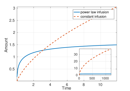
Figure 2: Amount-time profiles for $\alpha=0.5$: (solid line) amount of drug versus time according to Eq. (33) with constant infusion where there is unbounded accumulation of drug, (dashed line) time-profile according to Eq. (35), with power-law infusion where the amount of drug approaches a steady state. (Inset) The same profiles for $100$ times longer time span.

A two-compartment i.v. model

Based on the generalised approach for the fractionalisation of compartmental models, which allows mixing different fractional orders, developed above, a two-compartment fractional pharmacokinetic model is considered, shown schematically in Figure 3. Compartment 1 (central) represents general circulation and well perfused tissues while compartment 2 (peripheral) represents deeper tissues. Three transfer processes (fluxes) are considered: elimination from the central compartment and a mass flux from the central to the peripheral compartment, which are both assumed to follow classic kinetics (order 1), while a flux from the peripheral to the central compartment is assumed to follow slower fractional kinetics accounting for tissue trapping Petráš and Magin (2011); Dokoumetzidis and Macheras (2009).

The system is formulated mathematically as follows:

$$\frac{\mathrm{d}q_{1}(t)}{\mathrm{d}t} =-(k_{12}+k_{10})q_{1}(t)+k_{21,f}{\,}_{0}^{\mathrm{c}}\mathrm{D}_{t}^{1-\alpha}q_{2}(t),$$ (36a)

$$\frac{\mathrm{d}q_{2}(t)}{\mathrm{d}t} =k_{12}q_{1}(t)-k_{21,f}{\,}_{0}^{\mathrm{c}}\mathrm{D}_{t}^{1-\alpha}q_{2}(t),$$ (36b)

where $\alpha<1$ and initial conditions are $q_{1}(0)=q_{1,0}$, $q_{2}(0)=0$ which account for a bolus dose injection and no initial amount in the peripheral compartment. Note, that it is allowed to use Caputo derivatives here since the fractional derivatives involve only terms with $q_{2}$ for which there is no initial amount, which means that Caputo and RL derivatives are identical.

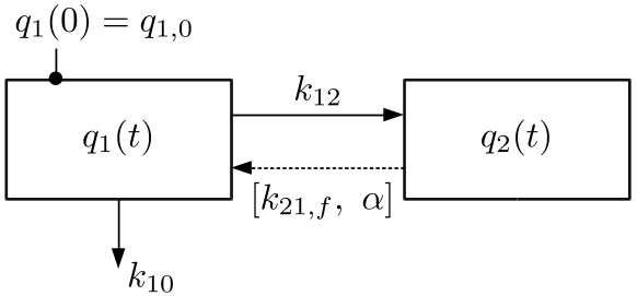
Figure 3: A fractional two-compartment PK model with an i.v. bolus. Elimination from the central compartment and a mass flux from the central to the peripheral compartment, which are both assumed to follow classic kinetics (order 1), while a flux from the peripheral to the central compartment is assumed to follow slower fractional kinetics, accounting for tissue trapping (dashed arrow).

Applying the Laplace transform, to the above system the following algebraic equations are obtained:

$$sQ_{1}(s)-q_{1}(0) =-(k_{12}+k_{10})Q_{1}(s)+k_{21}(s^{1-\alpha}Q_{2}(s)-s^{-\alpha}q_{2}(0)),$$ (37a)

$$sQ_{2}(s)-q_{2}(0) =k_{12}Q_{1}(s)-k_{21,f}(s^{1-\alpha}Q_{2}(s)-s^{-\alpha}q_{2}(0)).$$ (37b)

Solving for $Q_{1}(s)$ and $Q_{2}(s)$ and substituting the initial conditions,

$$Q_{1}(s) =\frac{q_{1,0}(s^{\alpha}+k_{21,f})}{(s+k_{12}+k_{10})(s^{\alpha}+k_{21,f})-k_{12}k_{21,f}}$$ (38a)

$$Q_{2}(s) =\frac{q_{1,0}s^{\alpha-1}k_{12}}{(s+k_{12}+k_{10})(s^{\alpha}+k_{21,f})-k_{12}k_{21,f}}$$ (38b)

Using the above expression for $Q_{1}$ and $Q_{2}$, Eq. (38a) and Eq. (38b), respectively, can be used to simulate values of $q_{1}(t)$ and $q_{2}(t)$ in the time domain by an NILT method. Note, that primarily, $q_{1}(t)$ is of interest, since in practice we only have data from this compartment. The output for $q_{1}(t)$ from this numerical solution may be combined with the following equation

$$c(t)=\frac{q_{1}(t)}{V},$$ (39)

where $c$ is the drug concentration in the blood and $V$ is the apparent volume of distribution. Eq. (39) can be fitted to pharmacokinetic data in order to estimate parameters $V$, $k_{10}$, $k_{12}$, $k_{21,f}$ and $\alpha$.

The closed-form analytical solution of Eq. (36), can be expressed in terms of an infinite series of generalised Wright functions as demonstrated in the book by Kilbas et al. Kilbas et al (2006), but these solutions are hard to implement and apply in practice. Moloni in Moloni (2015) derived analytically the inverse Laplace transform of $Q_{1}(s)$ as:

$$q_{1}(t) =q_{1,0}\sum_{n=0}^{\infty}(-1)^{n}k_{21,f}^{n}\sum_{l=0}^{n}\frac{k_{10}^{l}n!}{(n-l)!l!}\Big{(}t^{l+\alpha n}\mathcal{E}_{1,l+\alpha n+1}^{n+1}(-(k_{10}+k_{12})t)$$

$$+t^{l+\alpha(n+1)}\mathcal{E}_{1,l+\alpha(n+1)+1}^{n+1}(-(k_{10}+k_{12})t)\Big{)},$$ (40a)

while for $$Q_{2}$$ the inverse Laplace transform works out to be Moloni (2015):

$$q_{2}(t)=q_{1,0}k_{12}\sum_{n=0}^{\infty}(-1)^{n}k_{21,f}^{n}\sum_{l=0}^{n}\frac{k_{10}^{l}n!}{(n-l)!l!}t^{l+\alpha n}\mathcal{E}_{1,l+\alpha n+2}^{n+1}(-(k_{10}+k_{12})t).$$ (40b)

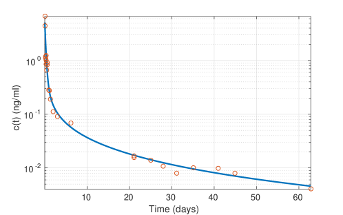
Figure 4: Concentration-time profile of amiodarone in the central compartment. The solid line corresponds to the fractional-order pharmacokinetic model of Eq. (36) with the parameter estimates: $\alpha=0.587$, $k_{10}=1.49\,\mathrm{days}^{-1}$, $k_{12}=2.95\,\mathrm{days}^{-1}$, $k_{21,f}=0.48\,\mathrm{days}^{-\alpha}$ and $\nicefrac{{q_{0}}}{{V}}=4.72\,\nicefrac{\mathrm{ng}}{\mathrm{ml}}$. The circles correspond to experimental measurements.

An application of the fractional two compartment model, the system of Eq. (36) to amiodarone PK data was presented in Dokoumetzidis et al (2010b). Amidarone is an antiarrhythmic drug known for its anomalous, non-exponential pharmacokinetics, which has important clinical implications due to the accumulation pattern of the drug in long-term administration. The fractional two-compartment model of the previous section was used to analyse an amiodarone i.v. data-set which first appeared in Holt et al (1983) and estimates of the model parameters were obtained. Analysis was carried out in MATLAB while the values for $q_{1}(t)$ of Eq. (40a) were simulated using a NILT algorithm De Hoog et al (1982) from the expression of $Q_{1}(s)$ in the Laplace domain. In Figure 4 the model-based predictions are plotted together the data demonstrating good agreement for the 60 day period of this study. The estimated fractional order was $\alpha=0.587$ and the non-exponential character of the curve is evident, while the model follows well the data both for long and for short times, unlike empirical power-laws which explode at $t=0$.

Numerical methods for fractional-order systems

For simple fractional-order models, as we discussed previously, there may exist closed-form analytical solutions which involve the one-parameter or two-parameters Mittage-Leffler function, or are given by more intricate analytical expressions such as Eq. (40). Interestingly, even for simple analytical solutions such as Eq. (16), the Mittag-Leffler function itself is evaluated by solving an FDE numerically Kaczorek (2011). This fact, without discrediting the value of analytical solutions, necessitates the availability of reliable numerical methods that allow us to simulate and study fractional-order systems. The availability of accurate discrete-time approximations of the trajectories of such systems is important not only for simulating, but also for the design of open-loop or closed-loop administration strategies, based on control theory Sopasakis et al (2015). Time-domain approximations are less parsimonious than $s$-domain ones, but are more suitable for control applications as we discuss in the next section.

There can be identified four types of solutions for fractional-order differential equations: (i) closed-form analytical solutions, (ii) approximations in the Laplace $s$-domain using integer-order rational transfer functions, (iii) numerical approximation schemes in the discrete time domain and (iv) numerical inverse Laplace transforms. Each of these comes with certain advantages as well as limitations; for example, closed-form analytical solutions are often not available, while the inverse Laplace function requires an explicit closed form for $u_{i}(t)$ so it cannot be used for administration rates that are defined implicitly or are arbitrary signals. Approximations in the $s$-domain are powerful modelling tools, but they fail to provide error bounds on the concentration of the administered drug in the time domain which are necessary in clinical practice.

In regard to closed-form analytical solutions, when available, they involve special functions such as the Mittag-Leffler function $\mathcal{E}_{\alpha,\beta}(t)=\sum_{k=0}^{\infty}{t^{k}}/{\Gamma(\alpha k+\beta)}$ whose evaluation calls, in turn, for some numerical approximation scheme. Analytical closed-form solutions of fractional differential equations are available for pharmacokinetic systems Verotta (2010). Typically for the evaluation of this function we resort to solving an FDE numerically Garrappa (2015); Seybold and Hilfer (2009); Gorenflo et al (2002) because the series in the definition of $\mathcal{E}_{\alpha,\beta}(t)$ converges rather slowly and no exact error bounds as available so as to establish meaningful termination criteria.

Transfer functions and integer-order approximations

Fractional-order systems, like their integer-order counterparts, can be modelled in the Laplace $s$-domain via transfer functions, that is,

$$F_{ij}(s)=\frac{Q_{j}(s)}{U_{i}(s)},$$ (41)

where $Q_{j}(s)$ and $U_{i}(s)$ are the Laplace transforms of the drug quantity $q_{j}(t)$ and the administration rate $u_{i}(t)$. If the pharmacokinetics is described by linear fractional-order models such as the ones discussed above, $F_{ij}$ will be a fractional-order rational function (a quotient of polynomials with real exponents).

Rational approximations aim at approximating such transfer functions — which involve terms of the form $s^{\alpha}$, $\alpha\in\mathbb{R}$ — by ordinary transfer functions of the form

$$\tilde{F}_{ij}(s)=\frac{P_{ij}(s)}{S_{ij}(s)},$$ (42)

where $P_{ij}$ and $S_{ij}$ are polynomials and the degree of $P_{ij}$ is no larger than the degree of $S_{ij}$. For convenience with notation, we henceforth drop the subscripts $ij$.

Padé Approximation: The Padé approximation of order $[m/n]$, $m,n\in\mathbb{N}$, at a point $s_{0}$ is rather popular and leads to rational functions with $\deg P=m$ and $\deg S=n$ Silva et al (2006).

Matsuda-Fujii continuous fractions approximation: This method consists in interpolating a function $F(s)$, which is treated as a black box, across a set of logarithmically spaced points Matsuda and Fujii (1993). By letting the selected points be $s_{k}$, $k=0,1,2,\dots$, the approximation is written as the continued fractions expansion

$$F(s)=\alpha_{0}+\frac{s-s_{0}}{\alpha_{1}+\frac{s-s_{1}}{\alpha_{2}+\frac{s-s_{2}}{\alpha_{3}+\dots}}}$$ (43)

where, $\alpha_{i}=\upsilon_{i}(s_{i})$, $\upsilon_{0}(s)=H(s)$ and $\upsilon_{i+1}(s)=\frac{s-s_{i}}{\upsilon_{i}(s)-\alpha_{i}}$.

Oustaloup’s method: Oustaloup’s method is based on the approximation of a function of the form:

$$H(s)=s^{\alpha},$$ (44)

with $\alpha>0$ by a rational function

$$\widehat{H}(s)=c_{0}\prod_{k=-N}^{N}\frac{s+\omega_{k}}{s+\omega^{\prime}_{k}},$$ (45)

within a range of frequencies from $\omega_{b}$ to $\omega_{h}$ Oustaloup et al (2000). The Oustaloup method offers an approximation at frequencies which are geometrically distributed about the characteristic frequency $\omega_{u}=\sqrt{\omega_{b}\omega_{h}}$ — the geometric mean of $\omega_{b}$ and $\omega_{h}$. The parameters $\omega_{k}$ and $\omega_{k}^{\prime}$ are determined via the design formulas Petráš (2011)

$$\omega_{k}^{\prime}=\omega_{b}\left(\frac{\omega_{h}}{\omega_{b}}\right)^{\frac{k+N+0.5(1+\alpha)}{2N+1}},$$ (46a)

$$\omega_{k}=\omega_{b}\left(\frac{\omega_{h}}{\omega_{b}}\right)^{\frac{k+N+0.5(1-\alpha)}{2N+1}},$$ (46b)

$$c_{0}=\left(\frac{\omega_{h}}{\omega_{b}}\right)^{-\frac{r}{2}}\prod_{k=-N}^{N}\frac{\omega_{k}}{\omega_{k}^{\prime}}.$$ (46c)

Parameters $\omega_{b}$, $\omega_{h}$ and $N$ are design parameters of the Oustaloup method.

There are a few more methods which have been proposed in the literature to approximate fractional-order systems by rational transfer functions such as Charef et al (1992); Carlson and Halijak (1964), as well as data-driven system identification techniques Gao and Liao (2012).

Time domain approximations

Several methods have been proposed which attempt to approximate the solution to a fractional-order initial value problem in the time domain.

Grünwald-Letnikov: This is the method of choice in the discrete time domain where ${{}^{\mathrm{gl}}\mathrm{D}}_{t}^{\alpha}x(t)$ is approximated by its discrete-time finite-history variant $({{{}^{\mathrm{gl}}\Delta}}^{\alpha}_{h,\nu}x)_{k}$ which is proven to have bounded error with respect to $({{{}^{\mathrm{gl}}\Delta}}_{h}^{\alpha}x)_{k}$ Sopasakis and Sarimveis (2017). The boundedness of this approximation error is a singular characteristic of this approximation method and is suitable for applications in drug administration where it is necessary to guarantee that the drug concentration in the body will remain within certain limits Sopasakis and Sarimveis (2017). As an example, system (15) is approximated (with sampling time $h$) by the discrete-time linear system

$$\tfrac{1}{h^{\alpha}}\sum_{j=0}^{\min\{\nu,\left\lfloor\nicefrac{{t}}{{h}}\right\rfloor\}}c_{j}^{\alpha}q_{k+1-j}=-k_{1,f}q_{k},$$ (47)

where $q_{k}=q(kh)$.

The discretisation of the Grünwald-Letnikov derivative suffers from the fact that the required memory grows unbounded with the simulation time. The truncation of the Grünwald-Letnikov series up to some finite memory gives rise to viable solution alorithms which can be elegantly described using triangular strip matrices as described in Podlubny (2000) and are available as a MATLAB toolbox.

Approximation by parametrisation: Approximate time-domain solutions can be obtained by assuming a particular parametric form for the solution. Such a method was proposed by Hennion and Hanert Hennion and Hanert (2013) where $q(t)$ is approximated by finite-length expansions of the form $\sum_{j=0}^{N}A_{j}\phi_{j}(t)$, where $\phi_{j}$ are Chebyshev polynomials and $A_{j}$ are constant coefficients. By virtue of the computability of fractional derivatives of $\phi_{j}$, the parametric approximation is plugged into the fractional differential equation which, along with the initial conditions, yields a linear system. What is notable in this method is that expansions as short as $N=10$ lead to very low approximation errors. Likewise, other parametric forms can be used. For example, Zainal and Kılıçman (2014) used a Fourier-type expansion and Kumar and Agrawal (2006) used piecewise quadratic functions.

Numerical integration methods: Fractional-order initial value problems can be solved with various numerical methods such as the Adams-Bashforth-Moulton predictor-corrector (ABMPC) method Zayernouri and Matzavinos (2016) and fractional linear multi-step methods (FLMMs) Lubich (1986); Garrappa (2015). These methods are only suitable for systems of FDEs in the form

$${}_{0}^{\mathrm{c}}\mathrm{D}_{t}^{\gamma}x(t) =f(t,x(t)),$$ (48a)

$$x^{(k)}(0) =x_{0,k},\,k=0,\dots,m-1$$ (48b)

where $\gamma$ is a rational, and $m=\lceil\gamma\rceil$. Typically in pharmacokinetics we encounter cases with $0<\gamma\leq 1$, therefore, we will have $m=1$.

Let us give an example on how this applies to the two-compartment model we presented above. In order to bring Eq. (36) in the above form, we need to find a rational approximation of two derivatives, $1-\alpha$ and $1$. If we can find a satisfying rational approximation of $1-a\approxeq p/q$, then the first order derivative follows trivially. Now, Eq. (36) can be written as

$${}_{0}^{\mathrm{c}}\mathrm{D}_{t}^{\gamma}x_{0} =x_{1}$$ (49a)

$${}_{0}^{\mathrm{c}}\mathrm{D}_{t}^{\gamma}x_{1} =x_{2}$$ (49b)

$$\ \,\vdots$$

$${}_{0}^{\mathrm{c}}\mathrm{D}_{t}^{\gamma}x_{q-1} =-(k_{12}+k_{10})x_{0}{+}k_{21,f}x_{q+p}{+}u$$ (49c)

$${}_{0}^{\mathrm{c}}\mathrm{D}_{t}^{\gamma}x_{q} =x_{q+1}$$ (49d)

$$\ \,\vdots$$

$${}_{0}^{\mathrm{c}}\mathrm{D}_{t}^{\gamma}x_{2q-1} =k_{12}x_{0}-k_{21,f}x_{q+p}$$ (49e)

with initial conditions $x_{0}(0)=q_{1}(0)$, $x_{q}(0)=q_{2}(0)$ and $x_{i}(0)=0$ for $i\notin\{1,q\}$, and $\gamma=1/q$. This system is in fact a linear fractional-order system for which closed-form analytical solutions are available (Kaczorek, 2011, Thm. 2.5). In particular, Eq. (49) can be written concisely in the form

$${}_{0}^{\mathrm{c}}\mathrm{D}_{t}^{\gamma}\mathbf{x}(t) =A\mathbf{x}(t)+Bu(t)$$ (50a)

$$\mathbf{x}(0) =\mathbf{x}_{0},$$ (50b)

where $\mathbf{x}=(x_{0},x_{1},\ldots,x_{2q-1})$ and $\mathbf{x}_{0}=(x_{0}(0),\ldots,x_{2q-1}(0))$ and matrices $A$ and $B$ can be readily constructed from the above dynamical equations. This fractional-order initial value problem has the closed-form analytical solution (Kaczorek, 2011, Thm. 2.5)

$$\mathbf{x}(t)=\mathcal{E}_{\gamma}(At^{\gamma})\mathbf{x}_{0}+\int_{0}^{t}\sum_{k=0}^{\infty}\frac{A^{k}(t-\tau)^{k\gamma}}{\Gamma((k+1)\gamma)}Bu(\tau)\mathrm{d}\tau.$$ (51)

Evidently, the inherent complexity of this closed-form analytical solution — which would require the evaluation of slowly-converging series — motivates and necessitates the use of numerical methods.

The number of states of system (49) is $2q$, therefore, the rational approximation should aim at a small $q$. Yet another reason to choose small $q$ is that small values of $\gamma$ render the system hard to simulate numerically because they increase the effect of and dependence on the memory.

Adams-Bashforth-Moulton predictor-corrector (ABMPC): Methods of the ABMPC type have been generalised to solve fractional-order systems. The key idea is to evaluate $({{{}_{0}^{\mathrm{rl}}\mathrm{I}}}^{\gamma}f)(t,x(t))$ by approximating $f$ with appropriately selected polynomials. Solutions of Eq. (48) satisfy the following integral representation

$$x(t)=\sum_{k=0}^{m-1}x_{0,k}\frac{t^{k}}{k!}+({{{}_{0}^{\mathrm{rl}}\mathrm{I}}}^{\gamma}f)(t,x(t)),$$ (52)

where the first term on right hand side will be denoted by $T_{m-1}(t).$ This is precisely an integral representation of Eq. (48). The integral on the right hand side of the previous equation can be approximated, using an uniformly spaced grid $t_{n}=nh$, by $\frac{h^{\gamma}}{\gamma(\gamma+1)}\sum_{j=0}^{n+1}a_{j,n+1}f(t_{j})$ for suitable coefficients $a_{j,n+1}$ Diethelm et al (2002). The numerical approximation of the solution of Eq. (48) is

$$x(t_{n+1}) =T_{m-1}(t_{n+1})+\tfrac{h^{\gamma}}{\Gamma(\gamma+2)}f(t_{n+1},x_{p}(t_{n+1}))+\sum_{j=1}^{n}a_{j,n+1}f(t_{j},x(t_{j})).$$ (53a)

The equation above is usually referred to as the corrector formula and $$x_{p}(t_{n+1})$$ is given by the predictor formula

$$x_{P}(t_{n+1})=T_{m-1}(t_{n}) +\tfrac{1}{\Gamma(\gamma)}\sum_{j=0}^{n}b_{j,n+1}f(t_{j},x(t_{j})).$$ (53b)

Unfortunately, the convergence error of ABMPC when $0<\gamma<1$ is $\mathcal{O}(h^{1+\gamma})$, therefore, a rather small step size $h$ is required to attain a reasonable approximation error. A modification of the basic predictor-corrector method with more favourable computational cost is provided in Garrappa (2010) for which the MATLAB implementation fde12 is available.

Lubich’s method: Fractional linear multi-step methods (FLMM) Lubich (1986) are a generalisation of linear multi-step methods (LMM) for ordinary differential equations. The idea is to approximate the Riemann-Liouville fractional-order integral operator (1) with a discrete convolution, known as a convolution quadrature, as

$$({{}_{0}^{\mathrm{rl}}\mathrm{I}}_{h}^{\gamma}f)(t)\approxeq h^{\gamma}\sum_{j=0}^{n}\omega_{n-j}f(t_{j})+h^{\gamma}\sum_{j=0}^{s}w_{n,j}f(t_{j}),$$ (54)

for $t_{j}=jh$, where ($w_{n,j}$) and ($\omega_{n}$) are independent of $h$. Surprisingly, the latter can be constructed from any linear multistep method for arbitrary fractional order $\gamma$ Lubich (1986). FLMM constructed this way will inherit the same convergence rate and at least the same stability properties as the original LMM method Lubich (1985).

A MATLAB implementation of Lubich’s method, namely flmm2 Garrappa (2015) which is based on Garrappa (2015) is available. However, these methods do not perform well for small $\gamma$. According to Herceg et al (2017), for the case of amiodarone, it is reported that values of $\gamma$ smaller than $0.1$ give poor results and often do not converge, while using a crude approximation given by $\gamma=1/5$, flmm2 was shown to outperform fde12 in terms of accuracy and stability at bigger step sizes $h$.

Numerical inverse Laplace

The inverse Laplace transform of a transfer function $F(s)$ — on the Laplace $s$-domain — is given by the complex integral

$$f(t)=\mathcal{L}^{-1}\{F\}(t)=\lim_{T\rightarrow\infty}\frac{1}{2\pi i}\int_{\sigma-iT}^{\sigma+iT}e^{st}F(s)\mathrm{d}s,$$ (55)

where $\sigma$ is any real number larger than the real parts of the poles of $F$. The numerical inverse Laplace (NILT) approach aims at approximating the above integral numerically. Such numerical methods apply also to cases where $F$ is not rational as it is the case with fractional-order systems (55).

In the approach of De Hoog et al., the integral which appears in Eq. (55) is cast as a Fourier transform which can then be approximated by a Fourier series followed by standard numerical integration (e.g., using the trapezoid rule) De Hoog et al (1982). Though quite accurate for a broad class of functions, these methods are typically very demanding from the computational point of view. An implementation of the above method is available online Hollenbeck (1998).

In special cases analytical inversion can be done by means of Mittag-Leffler function Lin and Lu (2013); Kexue and Jigen (2011). A somewhat different approach is taken by Valsa and Brančik (1998), where authors approximate $e^{st}$, the kernel of the inverse Laplace transformation, by a function of the form $\tfrac{e^{st}}{1+e^{-2a}e^{2st}}$ and choose $a$ appropriately so as to achieve an accurate inversion.

In general, numerical inversion methods can achieve high precision, but they are not suitable for control design purposes, especially for optimal control problems. Moreover, there is not one single method that gives the most accurate inversion for all types of functions. An overview of the most popular inversion methods used in engineering practice is given in Hassanzadeh and Pooladi-Darvish (2007).

Drug administration for fractional pharmacokinetics

Approaches for drug administration scheduling can be classified according to the desired objective into methods where (i) we aim at stabilising the concentration in certain organs or tissues towards certain desired values (set points) Sopasakis et al (2014) and (ii) the drug concentration needs to remain within certain bounds which define a therapeutic window Sopasakis et al (2015).

Another level of classification alludes to the mode of administration where we identify the (i) continuous administration by, for instance, intravenous continuous infusion, (ii) bolus administration, where the medicine is administered at discrete time instants Sopasakis et al (2015); Rivadeneira et al (2015) and (iii) oral administration where the drug is administered both at discrete times and from a discrete set of dosages (e.g., tablets) Sopasakis and Sarimveis (2012).

Drug administration is classified according to the way in which decisions are made in regard to how often, at what rate and/or what amount of drug needs to be administered to the patient. We can identify (i) open-loop administration policies where the patient follows a prescribed dosing scheme without adjusting the dosage and (ii) closed-loop administration where the dosage is adjusted according to the progress of the therapy Sopasakis et al (2014). The latter is suitable mainly for hospitalised patients who are under monitoring and where drug concentration measurements are available or the effect of the drug can be quantified. Such is the case of controlled anaesthesia Krieger and Pistikopoulos (2014). However, applications of closed-loop policies extend beyond hospitals, such as in the case of glucose control in diabetes Favero et al (2014).

Despite the fact that optimisation-based methods are well-established in numerous scientific disciplines along with their demonstrated advantages over other approaches, to date, empirical approaches remain popular Kannikeswaran et al (2016); Fukudo et al (2017); De Ocenda et al (2016); Savic et al (2017).

In the following sections we propose decision making approaches for optimal drug administration using as a benchmark a fractional two-compartment model using, arbitrarily and as a benchmark, the parameters values of amiodarone. We focus on the methodological framework rather than devising an administration scheme for a particular compound. We discuss three important topics in optimal administration of compounds which are governed by fractional pharmacokinetics. Next, we formulate the drug administration problem as an optimal control problem we prescribe optimal therapeutic courses to individuals with known pharmacokinetic parameters. Lastly, we design optimal administration strategies for populations of patients whose pharmacokinetic parameters are unknown or inexactly known. We present an advanced closed-loop controlled administration methodology based on model predictive control.

Individualised administration scheduling

In this section we present an optimal drug administration scheme based on the two-compartment fractional model of Eq. (36) and assuming that the drug is administered into the central compartment continuously. We will show that the same model and the same approach can be modified to form the basis for bolus administration.

In order to state the optimal control problem for optimal drug administration we first need to discretise the two-compartment model (36) with a (small) sampling time $t_{c}$

$$t_{c}^{-1}(x_{k+1}-x_{k})=Ax_{k}+F\,{{}^{\mathrm{gl}}\Delta}^{1-a}_{t_{c},\nu}x_{k}+Bu_{k}$$ (56)

where $x_{k}=\left[q_{1}(kt_{c})\,\,q_{2}(kt_{c})\right]^{\prime}$ and $u_{k}$ is the administration rate at the discrete time $k$. The left hand side of (56) corresponds to the forward Euler approximation of the first-order derivative, and we shall refer to $t_{c}=10^{-2}\,\mathrm{days}$ as the control sampling time. On the right hand side of (56), ${{}^{\mathrm{gl}}\Delta}^{1-a}_{t_{c},\nu}$ has replaced the fractional-order operator ${}_{0}^{\mathrm{c}}\mathrm{D}_{t}^{1-\alpha}$. Matrices $A,F$ and $B$ are

$$A=\begin{bmatrix}-(k_{12}+k_{10})&0\\ k_{21,f}&0\\ \end{bmatrix},F=\begin{bmatrix}0&k_{21,f}\\ 0&-k_{21,f}\\ \end{bmatrix},B=\begin{bmatrix}1\\ 0\\ \end{bmatrix}.$$ (57)

The discrete-time dynamic equations of the system can now be stated as

$$x_{k+1}=x_{k}+t_{c}\bigg{(}Ax_{k}+\frac{F}{t_{c}^{1-a}}\sum_{j=0}^{\nu}c_{j}^{1-a}x_{k-j}+Bu_{k}\bigg{)},$$ (58)

where $c_{j}^{\alpha}=(-1)^{j}\binom{\alpha}{j}$. By augmenting the system with past values as $\mathbf{x}_{k}=(x_{k},x_{k-1},\dots,x_{k-\nu+1})$ we can rewrite Eq. (58) as a finite-dimension linear system

$$\mathbf{x}_{k+1}=\hat{A}\mathbf{x}_{k}+\hat{B}u_{k}.$$ (59)

Matrices $\hat{A}$ and $\hat{B}$ are straightforward to derive and are given in Sopasakis and Sarimveis (2017). The therapeutic session will last for $N_{d}=Nt_{c}=7\,\mathrm{days}$ in total, where $N$ is called the prediction horizon. Since it is not realistic to administer the drug to the patient too frequently, we assume that the patient is to receive their treatment every $t_{d}=0.5\,\mathrm{days}$. The administration schedule must ensure that the concentration of drug in all compartments never exceeds the minimum toxic concentration limits while tracking the prescribed reference value as close as possible. To this aim we formulate the constrained optimal control problem Bertsekas (2017)

$$\min_{u_{0},\ldots,u_{N_{d}-1}}J =\sum_{k=0}^{\nicefrac{{N_{d}}}{{t_{c}}}+1}(x_{\mathrm{ref},k}-x_{k})^{\prime}Q(x_{\mathrm{ref},k}-x_{k})$$ (60a)

subject to the constraints

$$\mathbf{x}_{k+1} =\hat{A}\mathbf{x}_{k}+\hat{B}u_{j},\text{ for }\ kt_{c}=jt_{d}$$ (60b)

$$\mathbf{x}_{k+1} =\hat{A}\mathbf{x}_{k},\text{ otherwise}$$ (60c)

$$0 \leq x_{k}\leq 0.5$$ (60d)

$$0 \leq u_{j}\leq 0.5$$ (60e)

for $$k=0,\ldots,N j=0,\ldots,N_{d}-1$$; .

In the above formulation $x_{\mathrm{ref},k}$ is the desired drug concentration at time $k$ and operator ^′ denotes vector transposition. Any deviation from set point is penalised by a weight matrix $Q$, where here we chose $Q=\mathrm{diag}([0\;1])$. Note that we are tracking only the second state. Our underlying GL model has a relative history of $t_{c}\nu=5\,\mathrm{days}$. Optimal drug concentrations are denoted by $u^{\star}_{k}$, for $k=0,\dots,N_{d}-1$ and they correspond to dosages administered intravenously at times $kt_{d}$. In the optimal control formulation we have implicitly assumed that $t_{d}$ is an integer multiple of $t_{c}$, which is not restrictive since $t_{c}$ can be chosen arbitrarily. In Figure 5 we present the pharmacokinetic profile of a patient following the prescribed optimal administration course.

Finally, the problem in Eq. (60) is a standard quadratic problem with simple equality and inequality constraints that can be solved at low computational complexity. Such problems can be easily formulated in YALMIP Löfberg (2004) or ForBES Stella et al (2017) for MATLAB or CVXPY Diamond and Boyd (2016) for Python.

Figure 5: Drug administration scheduling via optimal control. The behaviour of the controlled system was simulated using the ABMPC method (dashed red line). The predicted pharmacokinetic profile using the Grünwald-Letnikov approximation (solid blue line) and fde12 are indistinguishable. The set-point on $q_{2}$ (dashed orange line) and the maximum allowed concentration (black solid lines) are shown in the figure.

The optimal control framework offers great flexibility in using arbitrary system dynamics, constraints on the administration rate and the drug concentration in the various compartments, and cost functions which encode the administration objectives.

The quadratic function which we proposed in Eq. (60) is certainly not the only admissible choice. For instance, other possible choices are

1. $J=\sum_{k=0}^{\nicefrac{{N_{d}}}{{t_{c}}}+1}(x_{\mathrm{ref},k}-x_{k})^{\prime}Q(x_{\mathrm{ref},k}-x_{k})+\beta u_{k}^{2}$, where we also penalise the total amount of drug that is administered throughout the prediction horizon,

2. $J=\sum_{k=0}^{\nicefrac{{N_{d}}}{{t_{c}}}+1}\mathrm{dist}^{2}(x_{k},[\underline{$x$},\bar{x}])$, where $[\underline{$x$},\bar{x}]$ is the therapeutic window and $\mathrm{dist}^{2}(\cdot,[\underline{$x$},\bar{x}])$ is the squared distance function defined as $\mathrm{dist}^{2}(x_{k},[\underline{$x$},\bar{x}])=\min_{z_{k}}\{\|x_{k}-z_{k}\|^{2};\ \underline{$x$}\leq z_{k}\leq\bar{x}\}$.

Administration scheduling for populations

In the previous section, we assumed that the pharmacokinetic parameters are known aiming at an individualised dose regimen. When designing an administration schedule for a population of patients — without the ability to monitor the distribution of the drug or the progress of the therapy — then $J$ becomes a function of the pharmacokinetic parameters (in our case $k_{10}$, $k_{12}$, $k_{21,f}$ and $\alpha$). That said, $J$ becomes a random quantity which follows an — often unknown or inexactly known — probability distribution. In order to formulate an optimal control problem we now need to extract a characteristic value out of the random quantity $J$. There are two popular ways to do so leading to different problem statements.

First, we may consider the maximum value of $J$, $\max J$, over all possible values of $k_{10}$, $k_{12}$, $k_{21,f}$ and $\alpha$. This leads to robust or minimax problem formulations which consist in solving Bertsekas (2017)

$$\min_{u_{0},\ldots,u_{N_{d}-1}}\max_{k_{10},k_{12},k_{21,f},\alpha}J(u_{0},\ldots,u_{N_{d}-1},k_{10},k_{12},k_{21,f},\alpha),$$ (61)

subject to the system dynamics and constraints. In Eq. (61), the maximum is taken with respect to the worst-case values of $k_{10}$, $k_{12}$, $k_{21,f}$ and $\alpha$, that is, their minimum and maximum values. Apparently, the minimax approach does not make use of any probabilistic or statistical information which is typically available for the model parameters. As a result, it is likely to be overly conservative and lead to poor performance.

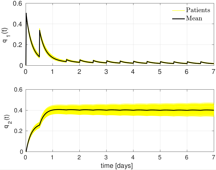
Figure 6: Drug administration to a population of $100$ (randomly generated) individuals by stochastic optimal control. The yellow thin lines correspond to the predicted individual responses to the administration and the black lines represent the average response.

On the other hand, in the stochastic approach we minimise the Bertsekas and Shreve (1996) expected cost $\mathbb{E}J$

$$\min_{u_{0},\ldots,u_{N_{d}-1}}\mathbb{E}_{k_{10},k_{12},k_{21,f},\alpha}\ J(u_{0},\ldots,u_{N_{d}-1},k_{10},k_{12},k_{21,f},\alpha),$$ (62)

subject to the system dynamics and constraints. Open-loop stochastic optimal control methodologies have been proposed for the optimal design of regimens under uncertainty for classical integer-order pharmacokinetics Schumitzky et al (1983); Lago (1992); Bayard et al (1994), yet, to the best of our knowledge, no studies have been conducted for the effectiveness of stochastic optimal control for fractional pharmacodynamics.

The expectation in Eq. (62) can be evaluated empirically given a data-set of estimated pharmacokinetic parameters $(k_{10}^{(i)},k_{12}^{(i)},k_{21,f}^{(i)},\alpha^{(i)})_{i=1}^{L}$ by minimising the sample average of $J$, that is

$$\min_{u_{0},\ldots,u_{N_{d}-1}}\tfrac{1}{L}\sum_{i=1}^{L}J(u_{0},\ldots,u_{N_{d}-1},k_{10}^{(i)},k_{12}^{(i)},k_{21,f}^{(i)},\alpha^{(i)}).$$ (63)

The effect of $L$ on the accuracy of the derived optimal decisions is addressed in Campi et al (2009) where probabilistic bounds are provided. Simulation results with the stochastic optimal control methodology on a population of $100$ patients using $L=20$ are shown in Figure 6. Note that in both the minimax and the stochastic approach, a common therapeutic course $u_{0},\ldots,u_{N_{d}-1}$ is sought for the whole population of patients.

In stochastic optimal control it is customary to adapt the state constraints in a probabilistic context requiring that they be satisfied with certain probability, that is

$$\mathrm{P}[x_{k}\leq x_{\max}]\geq 1-\beta,$$ (64)

where $\beta\in[0,1]$ is a desired level of confidence. Such constraints are known as chance constraints or probabilistic constraints. Such problems, unless restrictive assumptions are imposed on the distribution of $x_{k}$, lead to nonconvex optimisation problems and solutions can be approximated by Monte Carlo sampling methods (Shapiro et al, 2009, Sec. 5.7.1) or by means of convex relaxations known as ambiguous chance constraints where (64) are replaced by $\mathrm{AV@R}_{\beta}[x_{k}]\leq x_{\max}$, where $\mathrm{AV@R}_{\beta}[x_{k}]$ is the average value-at-risk of $x_{k}$ at level $\beta$ (Shapiro et al, 2009, Sec. 6.3.4).

The minimax and the expectation operator are the two “extreme” choices with the former relating to complete lack of probabilistic information and the latter coming with the assumption of exact knowledge of the underlying distribution of pharmacokinetic parameters. Other operators can be chosen to account for imperfect knowledge of that distribution, therefore, bridging the gap between minimax and stochastic optimal control. Suitable operators for optimal control purposes are the coherent risk measures which give rise to risk-averse optimal control which is the state of the art in optimsation under uncertainty Herceg et al (2017).

Model Predictive Control

Model predictive control fuses an optimal control open-loop decision making process with closed-loop control when feedback is available. Following its notable success and wide adoption in the industry, MPC has been proposed for several cases of drug administration for drugs that follow integer-order kinetics such as erythropoietin Gaweda et al (2008), lithium ions Sopasakis et al (2015), propofol for anaesthesia Ionescu et al (2008) and, most predominantly, insulin administration to diabetic patients Schaller et al (2016); Hovorka et al (2004); Toffanin et al (2013); Parker et al (1999).

In MPC, at every time instant, we solve an optimal control problem which produces a plan of future drug dosages over a finite prediction horizon by minimising a performance index $J$. The future distribution of the drug in the organism is predicted with a dynamical model such as the ones based on the Grünwald-Letnikov discretisation presented in the previous sections. Out of the planned sequence of dosages, the first one is actually administered to the patient. At the next time instant, the drug concentration is measured and the same procedure is repeated in a fashion known as receding horizon control Rawlings and Mayne (2009).

A fractional variant of the classical PID controller, namely a PI^λD^μ fractional-order controller, has been proposed in Sopasakis and Sarimveis (2014) for the controlled administration. However, the comparative advantage of MPC is that it can inherently account for administration rate, drug amount and drug concentration constraints which are of capital importance. In Sopasakis et al (2015); Sopasakis and Sarimveis (2017), the truncated Grünwald-Letnikov approximation serves as the basis to formulate MPC formulations with guaranteed asymptotic stability and satisfaction of the constraints at all time instants. We also single out impulsive MPC, which was proposed in Sopasakis et al (2015), which is particularly well-suited for applications of bolus administration where the patient is injected the medication (e.g., intravenously), thus abruptly increasing the drug concentration. In such cases, it is not possible to achieve equilibrium, but instead the objective becomes to keep the concentration within certain therapeutic limits. Model predictive control can further be combined with stochastic Patrinos et al (2014); Sopasakis et al (2017) and risk-averse Herceg et al (2017) optimal control aiming at a highly robust administration that is resilient to the inexact knowledge of the pharmacokinetic parameters of the patient as well as potential time varying phenomena (e.g., change in the PK/PD parameter values due to illness, drug-drug interactions and alternations due to other external influences).

Furthermore, in feedback control scenarios, state information is often partially available. For example, when a multi-compartment model is used, concentration measurement from only a single compartment is available. As an example, in the case of multi-compartment physiologically based models, we would normally only have information from the blood compartment. In such cases, a state observer can be used to produce estimates of concentrations or amounts of drug in compartments where we do not have access. A state observer is a dynamical system which, using observations of (i) those concentrations that can be measures and (ii) amount or rate of administered drug at every time instant, produces estimates $\hat{q}_{i}$ of those amounts/concentrations of drug to which we do not have access. State observers are designed so that $\hat{q}_{i}(t)-q_{i}(t)\to 0$ as $t\to\infty$, that is, although at the beginning (at $t=0$) we only have an estimate $\hat{q}_{i}(0)$ of $q_{i}(0)$, we shall eventually obtain better results which converge to the actual concentrations. State observers, such as the Kalman filter, have been successfully employed in the administration of compounds following integer-order dynamics Sopasakis et al (2014) including applications of artificial pancreas Patek et al (2007); Wang et al (2014).

Observers are, furthermore, employed to filter out measurement errors and modelling errors. When the system model is inexact, the system dynamics in Eq. (59) becomes

$$\mathbf{x}_{k+1}=\hat{A}\mathbf{x}_{k}+\hat{B}u_{k}+d_{k},$$ (65)

where $d_{k}$ serves as a model mismatch term. We may then assume that $d_{k}$ follows itself some dynamics often as trivial as $d_{k+1}=d_{k}$. We may then formulate the following linear dynamical system with state $(\mathbf{x}_{k},d_{k})$

$$\begin{bmatrix}\mathbf{x}_{k+1}\\ d_{k+1}\end{bmatrix}=\begin{bmatrix}\hat{A}&I\\ 0&I\end{bmatrix}\begin{bmatrix}\mathbf{x}_{k}\\ d_{k}\end{bmatrix}+\begin{bmatrix}\hat{B}\\ 0\end{bmatrix}u_{k},$$ (66)

and build a state observer for $(\mathbf{x}_{k},d_{k})$ jointly. The estimates $(\hat{\mathbf{x}}_{k},\hat{d}_{k})$ are then fed to the MPC. This leads to an MPC formulation known as offset-free MPC Sopasakis et al (2014) that can control systems with biased estimates of the pharmacokinetic parameters.

Model predictive control is a highly appealing approach because it can account for imperfect knowledge of the pharmacokinetic parameters of the patient, measurement noise, partial availability of measurements and constraints while it decides the amount of administered drug by optimising a cost function thus leading to unparalleled performance. Moreover, the tuning of MPC is more straightforward compared to other control approaches such as PID or fractional PID. In MPC the main tuning knob is the cost function $J$ of the involved optimal control problem which reflects and encodes exactly the control objectives.

Conclusions

Fractional kinetics offers an elegant description of anomalous kinetics, i.e., non-exponential terminal phases, the presence of which has been acknowledged in pharmaceutical literature extensively. The approach offers simplicity and a valid scientific basis, since it has been applied in problems of diffusion in physics and biology. It introduces the Mittag-Leffler function which describes power law behaved data well, in all time scales, unlike the empirical power-laws which describe the data only for large times. Despite the mathematical difficulties, fractional pharmacokinetics offer undoubtedly a powerful and indispensable approach for the toolbox of the pharmaceutical scientist.

Solutions of fractional-order systems involve Mittag-Leffler-type functions, or other special functions whose numerical evaluation is nontrivial. Several approximation techniques have been proposed as we outlined above for fractional systems with different levels of accuracy, parsimony and suitability for optimal administration scheduling or control. In particular, those based on discrete time-domain approximations of the system dynamics with bounded approximation error, such as the truncated Grünwald-Letnikov approximation, are most suitable for optimal control applications. There nowadays exist software that implement most of the algorithms that are available in the literature and facilitate their practical use. Further research effort needs to be dedicated in deriving error bounds in the time domain for available approximation methods that will allow their adoption in optimal control formulations.

The optimal control framework is suitable for the design of administration courses both to individuals as well as to populations where the intra-patient variability of pharmacokinetic parameters needs to be taken into account. In fact, stochastic optimal control offers a data-driven decision making solution that enables us to go from sample data to administration schemes for populations. Optimal control offers great flexibility in formulating optimal drug dosing problems and different problem structures arise naturally for different modes of administration (continuous, bolus intravenous, oral and more). At the same time, further research is necessary to make realistic assumptions and translate them into meaningful optimisation problems.

MPC methodologies are becoming popular for controlled drug administration. Yet, their potential for fractional-order pharmacokinetics and their related properties, especially in regard to stochastic systems and the characterisation of invariant sets, needs to be investigated.

Overall, at the intersection of fractional systems theory, pharmacokinetics, numerical analysis, optimal control and model predictive control, spring numerous research questions which are addressed in the context of mathematical pharmacology.

References

- West and Deering (1994) West BJ, Deering W (1994) Fractal physiology for physicists: Lévy statistics. Physics Reports 246(1):1–100
- Ionescu et al (2017) Ionescu C, Lopes A, Copot D, Machado J, Bates J (2017) The role of fractional calculus in modeling biological phenomena: A review. Communications in Nonlinear Science and Numerical Simulation 51:141 – 159, DOI http://dx.doi.org/10.1016/j.cnsns.2017.04.001
- Kopelman (1988) Kopelman R (1988) Fractal reaction kinetics. Science 241(4873):1620 – 1626
- Macheras (1996) Macheras P (1996) A fractal approach to heterogeneous drug distribution: calcium pharmacokinetics. Pharmaceutical research 13(5):663–670
- Pereira (2010) Pereira L (2010) Fractal pharmacokinetics. Computational and Mathematical Methods in Medicine 11:161–184
- Wise (1985) Wise ME (1985) Negative power functions of time in pharmacokinetics and their implications. Journal of pharmacokinetics and biopharmaceutics 13(3):309–346
- Tucker et al (1984) Tucker G, Jackson P, Storey G, Holt D (1984) Amiodarone disposition: polyexponential, power and gamma functions. European journal of clinical pharmacology 26(5):655–656
- Weiss (1999) Weiss M (1999) The anomalous pharmacokinetics of amiodarone explained by nonexponential tissue trapping. Journal of pharmacokinetics and biopharmaceutics 27(4):383–396
- Phan et al (2006) Phan G, Le Gall B, Deverre JR, Fattal E, Bénech H (2006) Predicting plutonium decorporation efficacy after intravenous administration of DTPA formulations: study of pharmacokinetic-pharmacodynamic relationships in rats. Pharmaceutical research 23(9):2030–2035
- Sokolov et al (2002) Sokolov IM, Klafter J, Blumen A (2002) Fractional kinetics. Physics Today 55(11):48–54
- Podlubny (1999) Podlubny I (1999) Fractional differential equations, Mathematics in Science and Engineering, vol 198. Academic Publisher, San Diego, California
- Magin (2004a) Magin RL (2004a) Fractional calculus in bioengineering, part 1. Critical Reviews™ in Biomedical Engineering 32(1):1–104
- Magin (2004b) Magin RL (2004b) Fractional calculus in bioengineering, part3. Critical Reviews™ in Biomedical Engineering 32(3 – 4):195–377
- Magin (2004c) Magin RL (2004c) Fractional calculus in bioengineering, part 2. Critical Reviews™ in Biomedical Engineering 32(2):105–194
- Butera and Paola (2014) Butera S, Paola MD (2014) A physically based connection between fractional calculus and fractal geometry. Annals of Physics 350:146 – 158, DOI http://dx.doi.org/10.1016/j.aop.2014.07.008
- Chen et al (2010) Chen W, Sun H, Zhang X, Korošak D (2010) Anomalous diffusion modeling by fractal and fractional derivatives. Computers & Mathematics with Applications 59(5):1754 – 1758, DOI http://dx.doi.org/10.1016/j.camwa.2009.08.020
- Metzler et al (1994) Metzler R, Glöckle WG, Nonnenmacher TF (1994) Fractional model equation for anomalous diffusion. Physica A: Statistical Mechanics and its Applications 211(1):13 – 24, DOI http://dx.doi.org/10.1016/0378-4371(94)90064-7
- Copot et al (2014) Copot D, Ionescu CM, Keyser RD (2014) Relation between fractional order models and diffusion in the body. In: IFAC World Congress, Cape Town, South Africa, vol 47, pp 9277–9282, DOI http://dx.doi.org/10.3182/20140824-6-ZA-1003.02138
- Gmachowski (2015) Gmachowski L (2015) Fractal model of anomalous diffusion. European Biophysics Journal 44(8):613–621, DOI 10.1007/s00249-015-1054-5
- Klafter and Sokolov (2011) Klafter J, Sokolov IM (2011) First Steps in Random Walks: From Tools to Applications. Oxford University Press
- Eirich (1990) Eirich FR (1990) The fractal approach to heterogeneous chemistry, surfaces, colloids, polymers, vol 28. John Wiley & Sons, New York, DOI https://doi.org/10.1002/pol.1990.140280608
- Dokoumetzidis and Macheras (2011) Dokoumetzidis A, Macheras P (2011) The changing face of the rate concept in biopharmaceutical sciences: from classical to fractal and finally to fractional. Pharmaceutical Research 28(5):1229–1232
- Dokoumetzidis and Macheras (2009) Dokoumetzidis A, Macheras P (2009) Fractional kinetics in drug absorption and disposition processes. Journal of pharmacokinetics and pharmacodynamics 36(2):165–178
- Kytariolos et al (2010) Kytariolos J, Dokoumetzidis A, Macheras P (2010) Power law IVIVC: An application of fractional kinetics for drug release and absorption. European Journal of Pharmaceutical Sciences 41(2):299–304
- Popović et al (2010) Popović JK, Atanacković MT, Pilipović AS, Rapaić MR, Pilipović S, Atanacković TM (2010) A new approach to the compartmental analysis in pharmacokinetics: fractional time evolution of diclofenac. Journal of pharmacokinetics and pharmacodynamics 37(2):119–134
- Popović et al (2011) Popović JK, Dolićanin D, Rapaić MR, Popović SL, Pilipović S, Atanacković TM (2011) A nonlinear two compartmental fractional derivative model. European journal of drug metabolism and pharmacokinetics 36(4):189–196
- Popović et al (2013) Popović JK, Poša M, Popović KJ, Popović DJ, Milošević N, Tepavčević V (2013) Individualization of a pharmacokinetic model by fractional and nonlinear fit improvement. European journal of drug metabolism and pharmacokinetics 38(1):69–76
- Popović et al (2015) Popović JK, Spasić DT, Tošić J, Kolarović JL, Malti R, Mitić IM, Pilipović S, Atanacković TM (2015) Fractional model for pharmacokinetics of high dose methotrexate in children with acute lymphoblastic leukaemia. Communications in Nonlinear Science and Numerical Simulation 22(1):451–471
- Copot et al (2013) Copot D, Chevalier A, Ionescu CM, De Keyser R (2013) A two-compartment fractional derivative model for propofol diffusion in anesthesia. In: IEEE International Conference on Control Applications, pp 264–269, DOI https://doi.org/10.1109/CCA.2013.6662769
- Verotta (2010) Verotta D (2010) Fractional dynamics pharmacokinetics-pharmacodynamic models. Journal of pharmacokinetics and pharmacodynamics 37(3):257–276
- Van der Graaf et al (2015) Van der Graaf PH, Benson N, Peletier LA (2015) Topics in mathematical pharmacology. Journal of Dynamics and Differential Equations 28(3-4):1337–1356, DOI 10.1007/s10884-015-9468-4
- Hennion and Hanert (2013) Hennion M, Hanert E (2013) How to avoid unbounded drug accumulation with fractional pharmacokinetics. Journal of Pharmacokinetics and Pharmacodynamics 40(6):691–700, DOI 10.1007/s10928-013-9340-2
- Samko et al (1993) Samko S, Kilbas A, Marichev O (1993) Fractional integral and derivatives. Gordon & Breach Science Publishers
- Deng and Deng (2014) Deng J, Deng Z (2014) Existence of solutions of initial value problems for nonlinear fractional differential equations. Applied Mathematics Letters 32:6 – 12, DOI http://dx.doi.org/10.1016/j.aml.2014.02.001
- Mainardi (2014) Mainardi F (2014) On some properties of the Mittag-Leffler function , completely monotone for with . Discrete and Continuous Dynamical Systems – Series B 19(7):2267–2278, DOI 10.3934/dcdsb.2014.19.2267
- Papadopoulou et al (2006) Papadopoulou V, Kosmidis K, Vlachou M, Macheras P (2006) On the use of the weibull function for the discernment of drug release mechanisms. International Journal of Pharmaceutics 309(1):44 – 50, DOI https://doi.org/10.1016/j.ijpharm.2005.10.044
- De Hoog et al (1982) De Hoog FR, Knight J, Stokes A (1982) An improved method for numerical inversion of Laplace transforms. SIAM Journal on Scientific and Statistical Computing 3(3):357–366
- Dokoumetzidis et al (2010a) Dokoumetzidis A, Magin R, Macheras P (2010a) A commentary on fractionalization of multi-compartmental models. Journal of pharmacokinetics and pharmacodynamics 37(2):203–207
- Dokoumetzidis et al (2010b) Dokoumetzidis A, Magin R, Macheras P (2010b) Fractional kinetics in multi-compartmental systems. Journal of Pharmacokinetics and Pharmacodynamics 37(5):507–524
- Popović et al (2013) Popović JK, Pilipović S, Atanacković TM (2013) Two compartmental fractional derivative model with fractional derivatives of different order. Communications in Nonlinear Science and Numerical Simulation 18(9):2507 – 2514, DOI http://dx.doi.org/10.1016/j.cnsns.2013.01.004
- Petráš and Magin (2011) Petráš I, Magin RL (2011) Simulation of drug uptake in a two compartmental fractional model for a biological system. Communications in Nonlinear Science and Numerical Simulation 16(12):4588 – 4595, DOI https://doi.org/10.1016/j.cnsns.2011.02.012
- Kilbas et al (2006) Kilbas AA, Srivastava HM, Trujillo JJ (2006) Theory and applications of fractional differential equations, vol 204. Elsevier Science Limited
- Moloni (2015) Moloni S (2015) Applications of fractional calculus to pharmacokinetics. Master’s thesis, University of Patras, Department of Mathematics, Patras, Greece
- Holt et al (1983) Holt DW, Tucker GT, Jackson PR, Storey GC (1983) Amiodarone pharmacokinetics. American Heart Journal 106(4):840–847, DOI http://dx.doi.org/10.1016/0002-8703(83)90006-6
- Kaczorek (2011) Kaczorek T (2011) Selected Problems of Fractional Systems Theory. Springer Berlin Heidelberg
- Sopasakis et al (2015) Sopasakis P, Ntouskas S, Sarimveis H (2015) Robust model predictive control for discrete-time fractional-order systems. In: IEEE Mediterranean Conference on Control and Automation, pp 384–389
- Verotta (2010) Verotta D (2010) Fractional compartmental models and multi-term Mittag–Leffler response functions. Journal of Pharmacokinetics and Pharmacodynamics 37(2):209–215, DOI 10.1007/s10928-010-9155-3
- Garrappa (2015) Garrappa R (2015) Numerical evaluation of two and three parameter Mittag-Leffler functions. SIAM Journal of Numerical Analysis 53:1350–1369, DOI http://doi.org/10.1137/140971191
- Seybold and Hilfer (2009) Seybold H, Hilfer R (2009) Numerical algorithm for calculating the generalized mittag-leffler function. SIAM Journal on Numerical Analysis 47(1):69–88, DOI 10.1137/070700280, URL https://doi.org/10.1137/070700280
- Gorenflo et al (2002) Gorenflo R, Loutchko J, Luchko Y (2002) Computation of the mittag-leffler function and its derivatives. Fractional Calculus & Applied Analysis 5:1–26
- Silva et al (2006) Silva M, Machado J, Barbosa R (2006) Comparison of different orders Padé fractional order PD0.5 control algorithm implementations. IFAC Proceedings Volumes 39(11):373–378
- Matsuda and Fujii (1993) Matsuda K, Fujii H (1993) H(infinity) optimized wave-absorbing control - analytical and experimental results. Journal of Guidance, Control, and Dynamics 16(6):1146–1153
- Oustaloup et al (2000) Oustaloup A, Levron F, Mathieu B, Nanot FM (2000) Frequency-band complex noninteger differentiator: characterization and synthesis. IEEE Transactions on Circuits and Systems I: Fundamental Theory and Applications 47(1):25–39
- Petráš (2011) Petráš I (2011) Fractional derivatives, fractional integrals, and fractional differential equations in matlab. In: Assi A (ed) Engineering Education and Research Using MATLAB, InTech, DOI http://doi.org/10.5772/19412
- Charef et al (1992) Charef A, Sun HH, Tsao YY, Onaral B (1992) Fractal system as represented by singularity function. IEEE Transactions on Automatic Control 37(9):1465–1470
- Carlson and Halijak (1964) Carlson G, Halijak C (1964) Approximation of fractional capacitors by a regular Newton process. IEEE Transactions on Circuits Theory 11(2):210–213, DOI https://doi.org/10.1109/TCT.1964.1082270
- Gao and Liao (2012) Gao Z, Liao X (2012) Rational approximation for fractional-order system by particle swarm optimization. Nonlinear Dynamic 67(2):1387–1395, DOI https://doi.org/10.1007/s11071-011-0075-6
- Sopasakis and Sarimveis (2017) Sopasakis P, Sarimveis H (2017) Stabilising model predictive control for discrete-time fractional-order systems. Automatica 75:24–31
- Podlubny (2000) Podlubny I (2000) Matrix approach to discrete fractional calculus. Fractional Calculus & Applied Analysis 3:359–386
- Zainal and Kılıçman (2014) Zainal NH, Kılıçman A (2014) Solving fractional partial differential equations with corrected fourier series method. Abstract and Applied Analysis 2014:1–5, DOI 10.1155/2014/958931
- Kumar and Agrawal (2006) Kumar P, Agrawal OP (2006) An approximate method for numerical solution of fractional differential equations. Signal Processing 86(10):2602–2610, DOI http://dx.doi.org/10.1016/j.sigpro.2006.02.007
- Zayernouri and Matzavinos (2016) Zayernouri M, Matzavinos A (2016) Fractional Adams-Bashforth/Moulton methods: An application to the fractional Keller-Segel chemotaxis system. Journal of Computational Physics 317:1–14
- Lubich (1986) Lubich C (1986) Discretized fractional calculus. SIAM Journal on Mathematical Analysis 17(3):704–719
- Garrappa (2015) Garrappa R (2015) Trapezoidal methods for fractional differential equations: Theoretical and computational aspects. Mathematics and Computers in Simulation 110:96–112
- Diethelm et al (2002) Diethelm K, Ford NJ, Freed AD (2002) A predictor-corrector approach for the numerical solution of fractional differential equations. Nonlinear Dynamic 29(1):3–22, DOI https://doi.org/10.1023/A:1016592219341
- Garrappa (2010) Garrappa R (2010) On linear stability of predictor-corrector algorithms for fractional differential equations. International Journal of Computer Mathematics 87(10):2281–2290, DOI http://doi.org/10.1080/00207160802624331
- Lubich (1985) Lubich C (1985) Fractional linear multistep methods for Abel-Volterra integral equations of the second kind. Mathematics of Computation 45(172):463–469
- Garrappa (2015) Garrappa R (2015) Software for fractional differential equations. https://www.dm.uniba.it/Members/garrappa/Software, accessed:
- Herceg et al (2017) Herceg D, Ntouskas S, Sopasakis P, Dokoumetzidis A, Macheras P, Sarimveis H, Patrinos P (2017) Modeling and administration scheduling of fractional-order pharmacokinetic systems. In: IFAC World Congress, Toulouse, France
- Hollenbeck (1998) Hollenbeck KJ (1998) INVLAP.M: A MATLAB function for numerical inversion of Laplace transforms by the de Hoog algorithm. http://www.mathworks.com/matlabcentral/answers/uploaded_files/1034/invlap.m, accessed:
- Lin and Lu (2013) Lin SD, Lu CH (2013) Laplace transform for solving some families of fractional differential equations and its applications. Advances in Difference Equations 2013(1):137
- Kexue and Jigen (2011) Kexue L, Jigen P (2011) Laplace transform and fractional differential equations. Applied Mathematics Letters 24(12):2019 – 2023
- Valsa and Brančik (1998) Valsa J, Brančik L (1998) Approximate formulae for numerical inversion of Laplace transforms. International Journal of Numerical Modelling: Electronic Networks, Devices and Fields 11(3):153–166
- Hassanzadeh and Pooladi-Darvish (2007) Hassanzadeh H, Pooladi-Darvish M (2007) Comparison of different numerical Laplace inversion methods for engineering applications. Applied Mathematics and Computation 189(2):1966 – 1981
- Sopasakis et al (2014) Sopasakis P, Patrinos P, Sarimveis H (2014) Robust model predictive control for optimal continuous drug administration. Computer Methods and Programs in Biomedicine 116(3):193–204, DOI http://dx.doi.org/10.1016/j.cmpb.2014.06.003
- Sopasakis et al (2015) Sopasakis P, Patrinos P, Sarimveis H, Bemporad A (2015) Model predictive control for linear impulsive systems. IEEE Transactions on Automatic Control 60:2277–2282, DOI http://dx.doi.org/10.1109/TAC.2014.2380672
- Rivadeneira et al (2015) Rivadeneira PS, Ferramosca A, González AH (2015) MPC with state window target control in linear impulsive systems. In: 5th IFAC Conference on Nonlinear Model Predictive Control NMPC 2015, vol 48, pp 507–512, DOI http://dx.doi.org/10.1016/j.ifacol.2015.11.329
- Sopasakis and Sarimveis (2012) Sopasakis P, Sarimveis H (2012) An integer programming approach for optimal drug dose computation. Computer Methods and Programs in Biomedicine 108(3):1022–1035, DOI http://dx.doi.org/10.1016/j.cmpb.2012.06.008
- Krieger and Pistikopoulos (2014) Krieger A, Pistikopoulos EN (2014) Model predictive control of anesthesia under uncertainty. Computers & Chemical Engineering 71:699 – 707, DOI https://doi.org/10.1016/j.compchemeng.2014.07.025
- Favero et al (2014) Favero SD, Bruttomesso D, Palma FD, Lanzola G, Visentin R, Filippi A, Scotton R, Toffanin C, Messori M, Scarpellini S, Keith-Hynes P, Kovatchev BP, DeVries JH, Renard E, Magni L, Avogaro A, and CC (2014) First use of model predictive control in outpatient wearable artificial pancreas. Diabetes Care 37(5):1212–1215, DOI 10.2337/dc13-1631
- Kannikeswaran et al (2016) Kannikeswaran N, Lieh-Lai M, Malian M, Wang B, Farooqi A, Roback MG (2016) Optimal dosing of intravenous ketamine for procedural sedation in children in the ED — a randomized controlled trial. The American Journal of Emergency Medicine 34(8):1347 – 1353, DOI https://doi.org/10.1016/j.ajem.2016.03.064
- Fukudo et al (2017) Fukudo S, Matsueda K, Haruma K, Ida M, Hayase H, Akiho H, Nakashima Y, Hongo M (2017) Optimal dose of ramosetron in female patients with irritable bowel syndrome with diarrhea: A randomized, placebo-controlled phase II study. Neurogastroenterology & Motility 29(6):e13,023, DOI 10.1111/nmo.13023
- De Ocenda et al (2016) De Ocenda VR, Almeida-Prieto S, Luzardo-Álvarez A, Barja J, Otero-Espinar F, Blanco-Méndez J (2016) Pharmacokinetic model of florfenicol in turbot (scophthalmus maximus): establishment of optimal dosage and administration in medicated feed. Journal of Fish Diseases 40(3):411–424, DOI 10.1111/jfd.12525
- Savic et al (2017) Savic R, Weiner M, MacKenzie W, Engle M, WC W, Johnson J, Nsubuga P, Nahid P, Nguyen N, Peloquin C, Dooley K, Dorman S (2017) Defining the optimal dose of rifapentine for pulmonary tuberculosis: Exposure-response relations from two phase II clinical trials. Clinical Pharmacology & Therapeutics 102(2):321–331, DOI 10.1002/cpt.634
- Bertsekas (2017) Bertsekas DP (2017) Dynamic Programming and Optimal Control, 4th edn. Athena Scientific, Nashua, USA
- Löfberg (2004) Löfberg J (2004) YALMIP: A toolbox for modeling and optimization in MATLAB. In: IEEE International Symposium on Computer Aided Control Systems Design, New Orleans, LA, USA, pp 284–289, DOI http://doi.org/10.1109/CACSD.2004.1393890
- Stella et al (2017) Stella L, Themelis A, Patrinos P (2017) Forward–backward quasi-newton methods for nonsmooth optimization problems. Computational Optimization and Applications 67(3):443–487, DOI 10.1007/s10589-017-9912-y, forBES Software available at https://github.com/kul-forbes/ForBES
- Diamond and Boyd (2016) Diamond S, Boyd S (2016) CVXPY: A Python-embedded modeling language for convex optimization. Journal of Machine Learning Research 17(83):1–5
- Bertsekas and Shreve (1996) Bertsekas DP, Shreve SE (1996) Stochastic Optimal Control: The Discrete-Time Case. Athena Scientific, Nashua, USA
- Schumitzky et al (1983) Schumitzky A, Milman M, Katz D, D’Argenio DZ, Jelliffe RW (1983) Stochastic control of pharmacokinetic systems. In: The Seventh Annual Symposium on Computer Applications in Medical Care, 1983. Proceedings., pp 222–225, DOI 10.1109/SCAMC.1983.764595
- Lago (1992) Lago P (1992) Open-loop stochastic control of pharmacokinetic systems: A new method for design of dosing regimens. Computers and Biomedical Research 25(1):85–100, DOI 10.1016/0010-4809(92)90037-b
- Bayard et al (1994) Bayard D, Milman M, Schumitzky A (1994) Design of dosage regimens: A multiple model stochastic control approach. International Journal of Bio-Medical Computing 36(1):103 – 115, DOI http://dx.doi.org/10.1016/0020-7101(94)90100-7
- Campi et al (2009) Campi MC, Garatti S, Prandini M (2009) The scenario approach for systems and control design. Annual Reviews in Control 33(2):149 – 157, DOI http://dx.doi.org/10.1016/j.arcontrol.2009.07.001
- Shapiro et al (2009) Shapiro A, Dentcheva D, Ruszczyński (2009) Lectures on stochastic programming: modeling and theory. SIAM
- Herceg et al (2017) Herceg D, Sopasakis P, Bemporad A, Patrinos P (2017) Risk-averse model predictive control. https://arxiv.org/abs/1704.00342
- Gaweda et al (2008) Gaweda AE, Jacobs AA, Aronoff GR, Brier ME (2008) Model predictive control of erythropoietin administration in the anemia of ESRD. American Journal of Kidney Diseases 51(1):71–79, DOI 10.1053/j.ajkd.2007.10.003
- Ionescu et al (2008) Ionescu CM, Keyser RD, Torrico BC, Smet TD, Struys MM, Normey-Rico JE (2008) Robust predictive control strategy applied for propofol dosing using BIS as a controlled variable during anesthesia. IEEE Transactions on Biomedical Engineering 55(9):2161–2170, DOI 10.1109/TBME.2008.923142
- Schaller et al (2016) Schaller S, Lippert J, Schaupp L, Pieber TR, Schuppert A, Eissing T (2016) Robust PBPK/PD-based model predictive control of blood glucose. IEEE Transactions on Biomedical Engineering 63(7):1492–1504, DOI 10.1109/TBME.2015.2497273
- Hovorka et al (2004) Hovorka R, Canonico V, Chassin L, Haueter U, Massi-Benedetti M, Federici M, Pieber T, Schaller H, Schaupp L, Vering T, Wilinska M (2004) Nonlinear model predictive control of glucose concentration in subjects with type 1 diabetes. Physiological Measurement 25(4):905–920, DOI 10.1088/0967-3334/25/4/010
- Toffanin et al (2013) Toffanin C, Messori M, Palma FD, Nicolao GD, Cobelli C, Magni L (2013) Artificial pancreas: Model predictive control design from clinical experience. Journal of Diabetes Science and Technology 7(6):1470–1483, DOI 10.1177/193229681300700607
- Parker et al (1999) Parker RS, Doyle FJ, Peppas NA (1999) A model-based algorithm for blood glucose control in type I diabetic patients. IEEE Transactions on Biomedical Engineering 46(2):148–157, DOI 10.1109/10.740877
- Rawlings and Mayne (2009) Rawlings J, Mayne D (2009) Model Predictive Control: Theory and Design. Nob Hill Publishing
- Sopasakis and Sarimveis (2014) Sopasakis P, Sarimveis H (2014) Controlled drug administration by a fractional PID. In: IFAC World Congress, Cape Town, South Africa, pp 8421–8426
- Patrinos et al (2014) Patrinos P, Sopasakis P, Sarmiveis H, Bemporad A (2014) Stochastic model predictive control for constrained discrete-time Markovian switching systems. Automatica 50(10):2504–2514, DOI http://dx.doi.org/10.1016/j.automatica.2014.08.031
- Sopasakis et al (2017) Sopasakis P, Herceg D, Patrinos P, Bemporad A (2017) Stochastic economic model predictive control for Markovian switching systems. In: IFAC World Congress
- Patek et al (2007) Patek SD, Breton MD, Chen Y, Solomon C, Kovatchev B (2007) Linear quadratic gaussian-based closed-loop control of type 1 diabetes. Journal of Diabetes Science and Technology 1(6):834–841
- Wang et al (2014) Wang Q, Molenaar P, Harsh S, Freeman K, Xie J, Gold C, Rovine M, Ulbrecht J (2014) Personalized state-space modeling of glucose dynamics for type 1 diabetes using continuously monitored glucose, insulin dose, and meal intake. Journal of Diabetes Science and Technology 8(2):331–345, DOI 10.1177/1932296814524080