A Rapid Fault Reconstruction Strategy Using a Bank of Sliding Mode Observers

Abstract

This paper deals with the design of a model-based rapid fault detection and isolation strategy using sliding mode observers. To address this problem, a new scheme is proposed by adaptively combining the information provided by a bank of observers. In this regard, a new structure for sliding mode observers is considered. Then, the well-known recursive least square algorithm is utilized to merge individual state estimations suitably such that the system fault is detected faster. The required condition for enhancing perfect state estimation is derived, and the stability of the overall system is proven via Lyapunov’s direct method. The supremacy of proposed scheme is fully discussed through mathematical analyses as well as simulations.

I Introduction

Reconstructing unknown inputs of a given process is of great significance from both practical and theoretical aspects. One example of unknown inputs is exogenous disturbances. It is well-known that if such disturbances are not identified and compensated properly, they will deteriorate performance of the closed-loop system. To tackle this problem, several disturbance observers have been developed in the control literature [1, 2, 3]. System components fault, which frequently occurs in engineering systems, is another example of unknown inputs. Occurrence of fault may cause irrecoverable damages and even failure of the whole process. To avoid such circumstances, one solution is to consider redundancy for critical components of the process and always check the signals provided by these duplicated components. By using such structures and employing a voting mechanism, it is possible to detect faulty signals, and in turn, select the appropriate signals. This strategy has been widely used in industries to obtain a process with high availability. Although such a simple approach has proven to provide reliable schemes in practice, one cannot turn a blind eye on the fact that it is costly and not energy efficient. Moreover, in some applications it is not possible to duplicate system components due to the nature of the understudy problem, space limitations, accumulation of noise, etc. To avoid such problems, in the past few decades, several attempts have been made to reconstruct faults using automatic strategies [4, 5, 6, 7]. In [5], Sliding Mode Observers (SMOs) are employed to design a model-based structure to reconstruct waste-gate faults in turbocharged gasoline engines. In [6], an algorithm is presented for fault detection in linear time-varying discrete systems using Luenberger observers. Partial kernel principle component analysis is employed for health monitoring of aero-derivative industrial turbines in [8].

Many existing methodologies in control literature assume that all system states are accessible [9]. However, this assumption is not always realistic. It is well-known that this issue can be addressed by employing suitable observers. In the past decades, several observers and observer-based strategies have been presented for linear and nonlinear systems [10, 11, 12, 13]. Among these observers, SMOs, which are capable of rejecting impacts of disturbances on the final estimations, have obtained great deal of attentions from fault detection community. This feature, disturbance rejection, is employed for fault detection, isolation, and input reconstruction in [14, 15, 16, 17].

On the other hand, it should be emphasized that not only does late detection of such malfunctions cause fault propagation and failure of the whole process, but it also put the process operators’ lives in jeopardy. Hence, early detection of such malfunctions has received a considerable attention, and several attempts have been made to design rapid fault detection methodologies [18, 19, 20]. In [18], an intelligent modular method is proposed for fast fault detection and classification in power systems. A robust fast fault detection approach is presented for T-S fuzzy systems in [19]. Assuming the time derivative of system output, $\dot{y}(t)$, is available for measurement; an algorithm is presented for rapid actuator fault detection in [20]. On the other hand, it is well-known that by using multiple observers one can estimate system states with better transient response [21, 22], which can be employed for fault detection purposes. In [23], a new identification scheme is presented for Linear Time Invariant (LTI) systems in order to improve the parameter estimation performance. In this regard, a convex combination of all information provided by multiple models is utilized to estimate system unknown parameters. Applying this idea to different systems with unknown parameters (e.g., LTI systems [24], linear systems with unknown periodic parameters [25, 26], nonlinear systems [27, 28], and twin-rotor system [29]) has shown that this approach is also capable of providing satisfactory performance in various cases.

In this paper, a novel fault reconstruction scheme is presented using a convex combination of the state estimations obtained from a bank of SMOs. The method is composed of a new structure for multiple SMOs and the Recursive Least Squares (RLS) algorithm. The main contributions of this paper are as follows: I) A new structure for state estimation of systems with unknown inputs is presented by adaptively combining multiple SMOs state estimations. II) Using the properties of convex combination, the existence of some unknown constant parameters that provide a perfect state estimation is guaranteed. III) The stability of the proposed scheme, consisting of interconnection of multiple dynamical systems, is investigated, and it is proved that the estimations converge to the actual values. IV) The mathematical performance analysis of the proposed scheme is provided which shows that the presented strategy is capable of resulting in a better transient response in comparison to the conventional SMOs. V) The presented fault reconstruction methodology does not require accessibility of all system states.

The remainder of paper is structured as follows: The problem statement and SMO are presented in Section 2. In Section 3, the proposed observer scheme is introduced; then, the existence of a perfect state estimation is assured. Furthermore, the stability of proposed structure and its performance are also discussed in this section. Simulation results are included in Section 4, and finally, Section 5 provides the conclusions.

II Sliding Mode Observers

Consider the following uncertain system

$$\begin{split}\dot{x}&=Ax+Bu+D\xi(t,x,u),\\ y&=Cx,\end{split}$$ (1)

where $x\in{\mathcal{R}}^{n}$ is the state vector, $u\in\mathcal{R}^{m}$ is the bounded control input which stabilizes the system, $y\in\mathcal{R}^{p}$ is the system output, and $\xi(t,x,u)\in\mathcal{R}^{q}$ denotes an unknown bounded function satisfying the following inequality

$$\|\xi(t,x,u)\|\leq\overline{\xi},$$ (2)

Moreover, it is assumed that $p\geq q$ and $B$, $C$, and $D$ are full rank matrices [11].

To estimate the state of the system, a SMO with the following structure can be utilized

$$\begin{split}\dot{\hat{x}}&=A\hat{x}+Bu-G_{l}\tilde{y}+G_{n}\nu(\hat{x}),\\ \hat{y}&=C\hat{x},\end{split}$$ (3)

where $\hat{x}$ and $\hat{y}$ represent estimations of $x$ and $y$, respectively, $\tilde{y}=\hat{y}-y$ is the output estimation error, and $\nu$ is a discontinuous term about the hyperplane

$$\mathcal{S}_{o}=\{\tilde{x}\in\mathcal{R}^{n}:C\tilde{x}=0\};\tilde{x}=\hat{x}-x,$$

Moreover, $G_{l}\in\mathcal{R}^{n\times p}$ and $G_{n}\in\mathcal{R}^{n\times p}$ are gain matrices to be determined. Note that in order to estimate the system states precisely, it is needed to reject the effects of unknown term $\xi$ on $\hat{x}$. The following definitions, lemmas, and theorem are used throughout the paper.

Definition 1 ([30])

The Rosenbrock matrix $\mathbb{R}(s)$ of the system $(A,D,C)$ is given by

$$\mathbb{R}(s)=\begin{bmatrix}sI_{n}-A&D\\ C&0\end{bmatrix}$$ (4)

The values of $s_{0}$ such that $\text{rank}(\mathbb{R}(s_{0}))<n+q$ are called invariant zeros of the system $(A,D,C)$.

Definition 2 ([31])

A set $\mathcal{K}$ in a linear space $\mathcal{L}$ is called convex if the line segment $ab$ is contained in $\mathcal{K}$ for any elements $a,b\in\mathcal{K}$, i.e., $(1-\lambda)a+\lambda b\in\mathcal{K}$ for any pair $(a,b)\in\mathcal{K}$ and any $\lambda\in[0,1]$.

Lemma 1 ([31])

Let $a_{1},a_{2},\cdots,a_{m}\in\mathcal{L}$ where $\mathcal{L}$ is a linear space. The intersection of all convex sets in $\mathcal{L}$ containing $a_{i}$s is called the convex hull $\mathcal{K}$ of {$a_{i}(i=1,2,\cdots,m)$} and any element of which, $a^{\prime}$, can be expressed as follows:

$$a^{\prime}=\sum\limits_{i=1}^{m}\beta_{i}a_{i}$$

where $\beta_{i}\in[0,1]$ is a constant term satisfying $\sum\nolimits_{i=1}^{m}\beta_{i}=1$.

Lemma 2 ([32])

Let $F$ be a bounded linear operator on an arbitrary Banach space $\mathcal{L}$. If $\|F\|<1$, then $I-F$ has a bounded inverse as follows

$$(I-F)^{-1}=I+\sum_{k=1}^{\infty}F^{k}$$

Theorem 1 ([33])

Consider the uncertain system (1), SMO (3), and let

$$\nu(\hat{x})=\begin{cases}-\rho\frac{P_{2}\tilde{y}}{\|P_{2}\tilde{y}\|}&\text{if }\tilde{y}\neq 0\\ 0&\text{otherwise}\end{cases}$$

where $P_{2}\in\mathcal{R}^{p\times p}$ and $\rho\geq\overline{\xi}+\gamma_{0}$ with $\gamma_{0}>0$. Then there exist matrices $G_{l}$, $G_{n}$, and $P_{2}$ such that $A_{0}=A-G_{l}C$ is a Hurwitz matrix and the state estimation obtained from (3) converges to the state of the plant if and only if:

• $\text{rank}(CD)=q$.

• invariant zeros of the system $(A,D,C)$ lie in the open left-hand side of complex plane, i.e., $\text{rank}(\mathbb{R}(s))=n+q$ for all $s$ with non-negative real part.

In the sequel, it is assumed that the conditions of Theorem 1 are satisfied, and a new observation scheme with more preferable performance is presented.

III The Main Results

In this section, the structure of the proposed observation scheme and its performance are fully discussed. Then, by utilizing the presented observation strategy, the unknown input reconstruction scheme as well as its stability analysis are addressed.

III-A Structure of the Proposed Multiple Sliding Mode Observer

In order to estimate the system states precisely with better transient response, the estimated states are provided by combining the observations obtained from multiple SMOs.

The proposed observer scheme is composed of $N$ SMOs with the following dynamics,

$$\begin{split}\dot{\hat{x}}_{i}(\alpha,t)&=A\hat{x}_{i}(\alpha,t)+Bu(t)-G_{l}\tilde{y}_{i}(\alpha,t)\\ &+G_{n}\nu(\sum\limits_{i=1}^{N}\alpha_{i}\hat{x}_{i}(\alpha,t),t),\\ \hat{y}_{i}(\alpha,t)&=C\hat{x}_{i}(\alpha,t),\end{split}$$ (5)

where $i=1,2,\cdots,N$ ($N\geq n+1$), $\tilde{y}_{i}(\alpha)=\hat{y}_{i}(\alpha)-y$ , $\hat{x}_{i}(\alpha,0)=\hat{x}_{i}(0)$, and

$$\nu(\sum\limits_{i=1}^{N}\alpha_{i}\hat{x}_{i}(\alpha))=\begin{cases}-\rho\frac{P_{2}\sum\limits_{i=1}^{N}\alpha_{i}\tilde{y}_{i}(\alpha)}{\|P_{2}\sum\limits_{i=1}^{N}\alpha_{i}\tilde{y}_{i}(\alpha)\|}&\text{if }\sum\limits_{i=1}^{N}\alpha_{i}\tilde{y}_{i}(\alpha)\neq 0,\\ 0&\text{otherwise},\end{cases}$$

with $0\leq\alpha_{i}\leq 1$, $\sum\nolimits_{i=1}^{N}{\alpha_{i}}=1$, and $\alpha=\begin{bmatrix}\alpha_{1}&\alpha_{2}&\cdots&\alpha_{N}\end{bmatrix}^{T}$. To use the full information provided by the aforementioned $N$ observers and obtain promising estimation, the final state estimation $\hat{x}_{o}$ is considered as a convex combination of the above estimations, i.e.,

$$\hat{x}_{o}(t)=\sum\limits_{i=1}^{N}\alpha_{i}\hat{x}_{i}(\alpha,t).$$ (6)

In the sequel, the analysis is divided into two parts: the algebraic part and the analytic part. In the former part, it is guaranteed that there exist unknown fixed $\alpha_{i}^{*}$s such that by choosing $\alpha_{i}=\alpha_{i}^{*}$s the perfect state estimation is obtained. The latter part covers derivation of appropriate adaptive laws for estimating these parameters. The following lemma is presented to obtain the required condition for the existence of $\alpha_{i}^{*}$s.

Lemma 3

If the initial conditions of $N$ ($N\geq n+1$) SMOs with the structure of (5), $\hat{x}_{i}(0)$s, are chosen such that the initial condition of the uncertain system (1), $x(0)$, lies in their convex hull $\mathcal{K}$, then there exist some fixed $\alpha_{i}^{*}$s such that

$$x(t)=\sum\limits_{i=1}^{N}\alpha_{i}^{*}\hat{x}_{i}(\alpha^{*},t)$$ (7)

where $0\leq\alpha_{i}^{*}\leq 1$, $\sum\nolimits_{i=1}^{N}{\alpha_{i}^{*}}=1$, and $\alpha^{*}=\begin{bmatrix}\alpha_{1}^{*}&\alpha_{2}^{*}&\cdots&\alpha_{N}^{*}\end{bmatrix}^{T}$.

Proof. There exists a change of coordinates, using a non-singular matrix $J$ that transforms the triple $(A,D,C)$ of system (1) to new coordinates $(\mathcal{A},\mathcal{D},\mathcal{C})$ such that [33]:

$$\begin{split}\dot{x}_{I}&=\mathcal{A}_{11}x_{I}+\mathcal{A}_{12}y+\mathcal{B}_{1}u\\ \dot{y}&=\mathcal{A}_{21}x_{I}+\mathcal{A}_{22}y+\mathcal{B}_{2}u+\mathcal{D}_{2}\xi\end{split}$$ (8)

where $x_{I}\in\mathcal{R}^{(n-p)}$, $y\in\mathcal{R}^{p}$, $\mathcal{A}=JAJ^{-1}$, $\mathcal{B}=JB$, $\mathcal{C}=CJ^{-1}$, $\mathcal{D}=JD$, and $\mathcal{A}_{11}$ is a stable matrix. On the other hand by using (5), (6), and the fact that $\alpha_{i}$s are constant, one can obtain the dynamics of state estimation as

$$\begin{split}\dot{\hat{x}}_{o}&=A\hat{x}_{o}+Bu-G_{l}\tilde{y}_{o}+G_{n}\nu(\hat{x}_{o}),\\ \hat{y}_{o}&=C\hat{x}_{o},\end{split}$$ (9)

where $\tilde{y}_{o}=\hat{y}_{o}-y$, $\hat{x}_{o}(0)=\sum_{i=1}^{N}\alpha_{i}\hat{x}_{i}(0)$, and

$$\nu(\hat{x}_{o})=\begin{cases}-\rho\frac{P_{2}\tilde{y}_{o}}{\|P_{2}\tilde{y}_{o}\|}&\text{if }\tilde{y}_{o}\neq 0,\\ 0&\text{otherwise}.\end{cases}$$

Similarly, the following dynamics can be obtained from (9) using the aforementioned transition matrix $J$:

$$\begin{split}\dot{\hat{x}}_{I}&=\mathcal{A}_{11}\hat{x}_{I}+\mathcal{A}_{12}\hat{y}+\mathcal{B}_{1}u(t)-\mathcal{G}_{l1}\tilde{y}_{o}\\ \dot{\hat{y}}&=\mathcal{A}_{21}\hat{x}_{I}+\mathcal{A}_{22}\hat{y}+\mathcal{B}_{2}u(t)-\mathcal{G}_{l2}\tilde{y}_{o}+\mathcal{G}_{n2}\nu\end{split}$$ (10)

where $\mathcal{G}_{l}=\begin{bmatrix}\mathcal{G}_{l1}^{T}&\mathcal{G}_{l2}^{T}\end{bmatrix}^{T}=JG_{l}$ and $\mathcal{G}_{n}=\begin{bmatrix}0&\mathcal{G}_{n2}^{T}\end{bmatrix}^{T}=JG_{n}$. Let us select the design parameters as

$$\begin{split}\mathcal{G}_{l1}=\mathcal{A}_{12},\quad\mathcal{G}_{l2}=\mathcal{A}_{22}-\mathcal{A}_{22}^{s},\quad\mathcal{G}_{n2}=\|\mathcal{D}_{2}\|I_{p}\end{split}.$$ (11)

where $\mathcal{A}_{22}^{s}$ is a design Hurwitz matrix. Now, a Lyapunov function candidate as $V(\tilde{x}_{I},\tilde{y}_{o})=\tilde{x}_{I}^{T}P_{1}\tilde{x}_{I}+\tilde{y}_{o}^{T}P_{2}\tilde{y}_{o}$ with $\tilde{x}_{I}=\hat{x}_{I}-x_{I}$ can be considered. In addition, two symmetric positive definite design matrices are defined as $Q_{1}\in\mathcal{R}^{(n-p)\times(n-p)}$ and $Q_{2}\in\mathcal{R}^{p\times p}$, and $P_{1}$ and $P_{2}$ are the symmetric positive definite matrices that satisfy the following Lyapunov equations

$$P_{2}\mathcal{A}_{22}^{s}+(\mathcal{A}_{22}^{s})^{T}P_{2} =-Q_{2}$$ (12)

$$P_{1}\mathcal{A}_{11}+\mathcal{A}_{11}^{T}P_{1} =-(\mathcal{A}_{21}^{T}P_{2}Q_{2}^{-1}P_{2}\mathcal{A}_{21}+Q_{1})$$

Then, following a procedure similar to what presented in [33], it can be shown that $\dot{V}<0$, and in turn, one can conclude that

$$V(t)<V(0)$$ (13)

To show that there exist some $\alpha_{i}^{*}$s satisfying (7), one can employ the transformation matrix $J$ and rewrite the Lyapunov function $V$ as follows:

$$\begin{split}V&=\tilde{x}_{o}^{T}P\tilde{x}_{o},\\ P&=J^{T}\begin{bmatrix}P_{1}&0\\ 0&P_{2}\end{bmatrix}J\end{split}$$ (14)

where $\tilde{x}_{o}=\hat{x}_{o}-x$ is the observation error. By considering the equation of

$$\underline{\lambda}(P)\tilde{x}_{o}^{T}\tilde{x}_{o}\leq V\leq\overline{\lambda}(P)\tilde{x}_{o}^{T}\tilde{x}_{o},$$ (15)

where $\underline{\lambda}(P)$ and $\overline{\lambda}(P)$ respectively are the smallest and largest eigenvalues of $P$, one can rewrite (13) as

$$\|\tilde{x}_{o}(t)\|\leq\sqrt{\frac{\overline{\lambda}(P)}{\underline{\lambda}(P)}}\|\tilde{x}_{o}(0)\|.$$ (16)

It is obvious that if $\tilde{x}_{o}(0)=0$, the right-hand side of the preceding inequality is zero, and consequently, $\tilde{x}_{o}(t)$ will maintain zero for all $t\geq 0$. Therefore, to conclude the proof, it is sufficient to find the conditions under which $\tilde{x}_{o}(t=0)$ is zero. Towards this end, one can use Lemma 1 and conclude that if the initial conditions of SMOs, i.e., $\hat{x}_{i}(0)$s, are chosen such that $x(0)$ is in the convex hull $\mathcal{K}$ of $\hat{x}_{i}(0)$s, then fixed $\alpha_{i}^{*}$s exist such that

$$x(0)=\sum\limits_{i=1}^{N}\alpha_{i}^{*}\hat{x}_{i}(0)$$

Hence, one can compare the preceding equation with (6) and see that the required condition for the perfect state estimation, $\tilde{x}_{o}(t=0)=0$, is satisfied. $\square$

It is worth noting that for $x(0)$ lies in the convex hull $\mathcal{K}$ of $\hat{x}_{i}(0)$s, one should at least utilize $N=n+1$ SMOs.

So far, it has been shown that there exist some $\alpha_{i}^{*}$s that provide perfect state estimation. However, these parameters are required to be estimated since they are unknown. Let us define $\tilde{x}_{i}=\hat{x}_{i}-x$, and use (7) and $\sum\nolimits_{i=1}^{N}\alpha_{i}^{*}=1$ to obtain $\sum\nolimits_{i=1}^{N}\alpha_{i}^{*}\tilde{x}_{i}(\alpha^{*},t)=0$. On the other hand, because $\alpha_{N}^{*}=1-\sum\nolimits_{i=1}^{N-1}\alpha^{*}_{i}$ and $\tilde{x}_{i}(\alpha^{*})-\tilde{x}_{N}(\alpha^{*})=\hat{x}_{i}(\alpha^{*})-\hat{x}_{N}(\alpha^{*})$, one can get

$$\sum\limits_{i=1}^{N-1}\alpha_{i}^{*}(\hat{x}_{i}(\alpha^{*},t)-\hat{x}_{N}(\alpha^{*},t))=-\tilde{x}_{N}(\alpha^{*},t)$$ (17)

Now, one can employ (5) to obtain

$$\dot{\hat{x}}_{i}(\alpha^{*},t)-\dot{\hat{x}}_{N}(\alpha^{*},t)=(A-G_{l}C)(\hat{x}_{i}(\alpha^{*},t)-\hat{x}_{N}(\alpha^{*},t))$$ (18)

It can be seen that $\hat{x}_{i}(\alpha^{*},t)-\hat{x}_{N}(\alpha^{*},t)$ is obtained from a linear system and in turn, only depends on $\hat{x}_{i}(0)-\hat{x}_{N}(0)$; therefore, if a matrix $E$ is considered such that its $i$th column is equal to $\hat{x}_{i}(\alpha^{*},t)-\hat{x}_{N}(\alpha^{*},t)$, it is independent of $\alpha^{*}$. As a result, (17) is rewritten as follows

$$E(t)\bar{\alpha}^{*}=-\tilde{x}_{N}(\bar{\alpha}^{*},t)$$ (19)

where $\bar{\alpha}^{*}=\begin{bmatrix}\alpha_{1}^{*}&\alpha_{2}^{*}&\cdots&\alpha_{N-1}^{*}\end{bmatrix}^{T}$. If $\tilde{x}_{N}(\alpha^{*})$ was known, the previous equation could be utilized for estimating $\bar{\alpha}^{*}$; however, it is unknown since $x$ and $\hat{x}_{N}(\bar{\alpha}^{*})$ are not available. Nonetheless, one can premultiply (19) by $C$ and get

$$CE(t)\bar{\alpha}^{*}=-\tilde{y}_{N}(\bar{\alpha}^{*},t)$$ (20)

Since $\hat{y}_{N}(\bar{\alpha}^{*})$ is unknown in the the preceding equation, the RLS algorithm cannot be employed for estimating $\bar{\alpha}^{*}$. However, it is proposed to employ a modification of the RLS algorithm as follows

$$\dot{\hat{\bar{\alpha}}}(t) =-R(t)E(t)^{T}C^{T}(CE(t)\hat{\bar{\alpha}}(t)+\tilde{y}_{N}(\hat{\bar{\alpha}}(t),t)),$$ (21)

$$\dot{R}(t) =-R(t)E(t)^{T}C^{T}CE(t)R(t),$$

where $\hat{\bar{\alpha}}(0)=\hat{\bar{\alpha}}_{0}$, $R(0)=\mu I$, $\hat{\bar{\alpha}}$ is an estimation of $\bar{\alpha}^{*}$, $\tilde{y}_{N}(\hat{\bar{\alpha}})=\hat{y}_{N}(\hat{\bar{\alpha}})-y$, $I$ is the identity matrix, and $\mu$ is a positive constant. Moreover, since $E(t)$ is independent of $\bar{\alpha}^{*}$, its $i$th column is considered as $\hat{x}_{i}(\hat{\bar{\alpha}}(t),t)-\hat{x}_{N}(\hat{\bar{\alpha}}(t),t)$. Even though $\tilde{y}_{N}(\hat{\bar{\alpha}})$ is employed instead of $\tilde{y}_{N}({\bar{\alpha}}^{*})$, it will be shown later that the previous equation is able to provide an estimation of $\bar{\alpha}^{*}$ suitable for estimating the state of the plant. Now, the obtained $\hat{\bar{\alpha}}$ can be exploited in the following SMOs for estimating the state variables

$$\begin{split}\dot{\hat{x}}_{i}(\hat{\bar{\alpha}})&=A\hat{x}_{i}(\hat{\bar{\alpha}})+Bu-G_{l}\tilde{y}_{i}(\hat{\bar{\alpha}})+G_{n}\nu(\hat{x}_{o}),\\ \hat{x}_{o}&=\sum\limits_{i=1}^{N-1}\hat{\alpha}_{i}\hat{x}_{i}(\hat{\bar{\alpha}})+(1-\sum\limits_{i=1}^{N-1}\hat{\alpha}_{i})\hat{x}_{N}(\hat{\bar{\alpha}})\end{split}$$ (22)

where $\tilde{y}_{i}(\hat{\bar{\alpha}})=C\hat{x}_{i}(\hat{\bar{\alpha}})-y$ and

$$\nu(\hat{x}_{o})=\begin{cases}-\rho\frac{P_{2}\sum\limits_{i=1}^{N}\hat{\alpha}_{i}\tilde{y}_{i}(\hat{\bar{\alpha}})}{\|P_{2}\sum\limits_{i=1}^{N}\hat{\alpha}_{i}\tilde{y}_{i}(\hat{\bar{\alpha}})\|}&\text{if }\sum\limits_{i=1}^{N}\hat{\alpha}_{i}\tilde{y}_{i}(\hat{\bar{\alpha}})\neq 0,\\ 0&\text{otherwise},\end{cases}$$

Now, it is required to investigate the stability of the proposed observation scheme, constructed from two interconnected systems (21) and (22), as well as the estimation error. In this regard, the following theorem is presented.

Theorem 2

For system (1), consider the modified RLS algorithm (21) and $N$ SMOs (22). If a non-singular matrix $J$ that transforms (1) to (8) is considered, the design matrices are chosen as

$$G_{l}=J^{-1}\begin{bmatrix}\mathcal{A}_{12}\\ \mathcal{A}_{22}-\mathcal{A}_{22}^{s}\end{bmatrix},G_{n}=\|\mathcal{D}_{2}\|J^{-1}\begin{bmatrix}0\\ I_{p}\end{bmatrix}$$ (23)

and $P_{2}$ satisfies (12), then it can be guaranteed that the observation error system is quadratically stable. Moreover, $\hat{x}_{i}$s are uniformly ultimately bounded, and $\hat{\bar{\alpha}}$ and $R$ are bounded.

Proof. Throughout the proof, it is required to employ the upper bounds of $\|E(t)\|$ and $\|R(t)\|$. In this regard, one can employ the definition of $E$ and (18) to obtain

$$\dot{E}(t)=A_{0}E(t)$$ (24)

where $A_{0}=A-G_{l}C$ is a Hurwitz matrix. Therefore, we have $E(t)=e^{A_{0}t}E(0)$, and $\|E(t)\|\leq\|e^{A_{0}t}\|\|E(0)\|$. In order to obtain an upper bound for $\|e^{A_{0}t}\|$, a Lyapunov function candidate $L=\operatorname{Tr}[e^{A_{0}^{T}t}P_{0}e^{A_{0}t}]$ with $P_{0}A_{0}+A_{0}^{T}P_{0}=-I$ is considered. Hence it can be obtained that $\dot{L}=-\operatorname{Tr}[e^{A_{0}^{T}t}e^{A_{0}t}]$. On the other hand, we have

$$\underline{\lambda}(P_{0})\operatorname{Tr}[e^{A_{0}^{T}t}e^{A_{0}t}]\leq L(t)\leq\overline{\lambda}(P_{0})\operatorname{Tr}[e^{A_{0}^{T}t}e^{A_{0}t}]$$ (25)

where $\underline{\lambda}(P_{0})$ and $\overline{\lambda}(P_{0})$ are the smallest and largest eigenvalues of $P_{0}$, respectively. One can use the preceding equation to get $\dot{L}\leq-({1}/{\overline{\lambda}(P_{0})})L$. Now, it is valid to say

$$L(t)\leq e^{-\frac{1}{\overline{\lambda}(P_{0})}t}L(0)$$

Moreover, by using (25), one has

$$\operatorname{Tr}[e^{A_{0}^{T}t}e^{A_{0}t}]\leq n\frac{\overline{\lambda}(P_{0})}{\underline{\lambda}(P_{0})}e^{-\frac{1}{\overline{\lambda}(P_{0})}t}$$

In addition, the equation $\|e^{A_{0}t}\|^{2}\leq\operatorname{Tr}[e^{A_{0}^{T}t}e^{A_{0}t}]$ can be employed for rewriting the preceding equation as follows

$$\|e^{A_{0}t}\|\leq ke^{-\lambda t}$$ (26)

where $k=\sqrt{n{\overline{\lambda}(P_{0})}/{\underline{\lambda}(P_{0})}}$ and $\lambda=1/(2\overline{\lambda}(P_{0}))$. By using the obtained upper bound of $\|e^{A_{0}t}\|$, we get

$$\|E(t)\|\leq ke^{-\lambda t}\|E(0)\|$$ (27)

For $R(t)$, the fact that it is a positive definite matrix can be employed. On the other hand, from (21) it can be seen that $\dot{R}(t)\leq 0$; therefore, by using $R(0)=\mu I$, we have $0\leq R(t)\leq\mu I$, i.e., $R(t)$ is bounded. Now it can be said that

$$\|R(t)\|\leq\mu$$ (28)

For obtaining the preceding equation, $\|R(t)\|^{2}=\overline{\lambda}(R(t))^{2}$ with the largest eigenvalue of $R(t)$ as $\overline{\lambda}(R(t))$ is employed, which is valid since $R(t)$ is a symmetric matrix.

Now, the obtained upper bounds can be used for proving the stability of the observation error system. In this regard, the state estimation (22) and the definition of $E$ can be utilized to obtain

$$\tilde{x}_{o}=E\hat{\bar{\alpha}}+\tilde{x}_{N}(\hat{\bar{\alpha}})$$ (29)

where $\tilde{x}_{o}=\hat{x}_{o}-x$ and $\tilde{x}_{N}=\hat{x}_{N}-x$. By using the previous equation and (21), we have

$$\dot{\hat{\bar{\alpha}}}=-RE^{T}C^{T}C\tilde{x}_{o}$$ (30)

Moreover, the observation error system of the $N$th observer can be obtained using (1) and (22) as follows

$$\dot{\tilde{x}}_{N}(\hat{\bar{\alpha}})=A_{0}\tilde{x}_{N}(\hat{\bar{\alpha}})+G_{n}\nu(\hat{x}_{o})-D\xi(t,x,u)$$ (31)

By taking the derivative of (29) and using (24), (30), and (31), one can obtain the observation error system as follows

$$\dot{\tilde{x}}_{o}=A_{0}\tilde{x}_{o}+G_{n}\nu(\hat{x}_{o})-D\xi(t,x,u)-ERE^{T}C^{T}C\tilde{x}_{o}$$ (32)

To show that the error system (32) is stable, let us start with the the following nominal error system

$$\dot{\tilde{x}}_{o}=A_{0}\tilde{x}_{o}+G_{n}\nu(\hat{x}_{o})-D\xi(t,x,u)$$

One can compare the preceding equation with the observation error system for the SMO (3) and see that they are the same. As a result, by choosing the design matrices as (23), the error system is quadratically stable [33]. Hence, there exists a Lyapunov function $V(\tilde{x}_{o})$ for the nominal error systems satisfying

$$\begin{split}c_{1}\|\tilde{x}_{o}\|^{2}\leq V(\tilde{x}_{o})&\leq c_{2}\|\tilde{x}_{o}\|^{2}\\ \frac{\partial V}{\partial t}+\frac{\partial V}{\partial\tilde{x}_{o}}[A_{0}\tilde{x}_{o}&+G_{n}\nu(\hat{x}_{o})-D\xi(t,x,u)]\leq-c_{3}\|\tilde{x}_{o}\|^{2}\\ \|\frac{\partial V}{\partial\tilde{x}_{o}}\|\leq c_{4}\|\tilde{x}_{o}\|\end{split}$$ (33)

for some positive constants $c_{1}$, $c_{2}$, $c_{3}$, and $c_{4}$ [34]. By considering $V(\tilde{x}_{o})$ as a Lyapunov function candidate for the observation error (32), one can get

$$\begin{split}\dot{V}(\tilde{x}_{o})&\leq\frac{\partial V}{\partial t}+\frac{\partial V}{\partial\tilde{x}_{o}}[A_{0}\tilde{x}_{o}+G_{n}\nu(\hat{x}_{o})-D\xi(t,x,u)]\\ &-\frac{\partial V}{\partial\tilde{x}_{o}}ERE^{T}C^{T}C\tilde{x}_{o}\end{split}$$

Using (33) and performing some basic manipulations on the preceding equation result in

$$\dot{V}(\tilde{x}_{o})\leq-c_{3}\|\tilde{x}_{o}\|^{2}+c_{4}\|E\|^{2}\|R\|\|C\|^{2}\|\tilde{x}_{o}\|^{2}$$

One can employ (27) and (28) to get

$$\dot{V}(\tilde{x}_{o})\leq-c_{3}\|\tilde{x}_{o}\|^{2}+c_{5}e^{-2\lambda t}\|\tilde{x}_{o}\|^{2}$$

where $c_{5}=c_{4}k^{2}\mu\|E(0)\|^{2}\|C\|^{2}$. By considering (33), we have

$$\dot{V}(\tilde{x}_{o})\leq(-\frac{c_{3}}{c_{2}}+\frac{c_{5}}{c_{1}}e^{-2\lambda t})V(\tilde{x}_{o})$$

Therefore, the following equation is satisfied

$$V(t)\leq e^{-\frac{c_{3}}{c_{2}}t}e^{\frac{c_{5}}{2\lambda c_{1}}(1-e^{-2\lambda t})}V(0)$$

Moreover, $e^{\frac{c_{5}}{2\lambda c_{1}}(1-e^{-2\lambda t})}\leq e^{\frac{c_{5}}{2\lambda c_{1}}}$; hence

$$V(t)\leq k_{1}e^{-\frac{c_{3}}{c_{2}}t}V(0)$$

where $k_{1}=e^{\frac{c_{5}}{2\lambda c_{1}}}$. Moreover, one can employ (33) and obtain

$$\|\tilde{x}_{o}(t)\|\leq k_{2}e^{-\frac{c_{3}}{2c_{2}}t}\|\tilde{x}_{o}(0)\|$$ (34)

with $k_{2}=\sqrt{k_{1}\frac{c_{2}}{c_{1}}}$. From the previous equation it can be concluded that the observation error converges to zero exponentially fast.

For proving the boundedness of $\hat{\bar{\alpha}}$, the integral of (30) is considered as follows

$$\hat{\bar{\alpha}}(t)=\hat{\bar{\alpha}}(0)-\int_{0}^{t}R(\tau)E(\tau)^{T}C^{T}C\tilde{x}_{o}(\tau)d\tau$$

Now, one can use (27), (28), and (34) to get

$$\begin{split}\|\hat{\bar{\alpha}}(t)\|&\leq\|\hat{\bar{\alpha}}(0)\|+\mu kk_{2}\|E(0)\|\|C\|^{2}\|\tilde{x}_{o}(0)\|\int_{0}^{t}e^{-\lambda\tau}e^{-\frac{c_{3}}{2c_{2}}\tau}d\tau\end{split}$$

By considering $\int_{0}^{t}e^{-\lambda\tau}e^{-\frac{c_{3}}{2c_{2}}\tau}d\tau\leq{2c_{2}}/(2\lambda c_{2}+c_{3})$, it can be seen that $\hat{\bar{\alpha}}$ is bounded.

For $\hat{x}_{i}(\hat{\bar{\alpha}})$s, one can consider the estimation error of the $i$th observer as $\tilde{x}_{i}=\hat{x_{i}}-x$ and a Lyapunov function candidate $V_{i}(\tilde{x}_{i}(\hat{\bar{\alpha}}))=\tilde{x}_{i}(\hat{\bar{\alpha}})^{T}P_{0}\tilde{x}_{i}(\hat{\bar{\alpha}})$ with $P_{0}A_{0}+A_{0}^{T}P_{0}=-I$. Therefore, by using (1) and (22) we can get

$$\begin{split}\dot{V}_{i}(\tilde{x}_{i}(\hat{\bar{\alpha}}))&\leq-\|\tilde{x}_{i}(\hat{\bar{\alpha}})\|^{2}+2\|\tilde{x}_{i}(\hat{\bar{\alpha}})\|\|P_{0}\|\\ &\times(\|G_{n}\|\|\nu(\hat{x}_{o})\|+\|D\|\|\xi\|)\end{split}$$

On the other hand, we have $\|\nu(\hat{x}_{o})\|\leq\rho$ and $\|\xi\|\leq\rho$. As a result, $\dot{V}_{i}(\tilde{x}_{i}(\hat{\bar{\alpha}}))<0$ for $\|\tilde{x}_{i}(\hat{\bar{\alpha}})\|>2\rho\|P_{0}\|(\|G_{n}\|+\|D\|)$. In other words, since $x$ is bounded, $\hat{x}_{i}$s are uniformly ultimately bounded. $\square$

The presented theorem states that the proposed observation scheme is able to provide a state estimation that converges to the state of the plant. In the next section, the performance of this observation scheme is investigated to obtain conditions that result in a better state estimation.

III-B Performance Investigation

This section is aimed at analyzing the performance of the proposed observer to see whether it is able to provide better state estimations than a single sliding mode observer. In order to investigate this improvement, the following lemma needs to be considered.

Lemma 4

For system (1), if the pair $(A,C)$ is observable, then the system $(A,D,C)$ has no invariant zero.

Proof. According to the Popov-Belevitch-Hautus rank test, the following matrix has full column rank since $(A,C)$ is observable

$$\mathbb{P}(s)=\begin{bmatrix}sI_{n}-A\\ C\end{bmatrix}$$

Therefore, $\text{rank}(\mathbb{P}(s))=n$. On the other hand, by considering the Rosenbrock matrix (4) and the fact that $D$ has full rank, one can conclude that $\text{rank}(\mathbb{R}(s))=\text{rank}(\mathbb{P}(s))+q$, which means there is no $s_{0}$ that makes $\mathbb{R}(s_{0})$ lose rank. $\square$

It can be seen from Lemma 4 that if $\text{rank}(CD)=q$ and $(A,C)$ is observable, the conditions of Theorem 1 are satisfied, and in turn, the results of the previous sections are still valid. As a result, in this section, it is assumed that the pair $(A,C)$ is observable. In addition, we assume that $x(0)$ is in the convex hull $\mathcal{K}$ of $\hat{x}_{i}(0)$s; hence (19) is satisfied, and one can rewrite (29) as follows

$$\tilde{x}_{o}=E\tilde{\bar{\alpha}}+\hat{x}_{N}(\hat{\bar{\alpha}})-\hat{x}_{N}({\bar{\alpha}}^{*})$$ (35)

where $\tilde{\bar{\alpha}}=\hat{\bar{\alpha}}-{\bar{\alpha}}^{*}$. For analyzing the preceding equation, the definition of $\nu$ and the fact that by choosing $\alpha_{i}=\alpha_{i}^{*}$s, the equality $\hat{x}_{o}(t)=x(t)$ is valid, can be considered to get

$$\dot{\hat{x}}_{N}({\bar{\alpha}}^{*})=A\hat{x}_{N}({\bar{\alpha}}^{*})+Bu-G_{l}e_{N}({\bar{\alpha}}^{*})$$

Therefore, we have

$$\frac{d}{dt}[\hat{x}_{N}(\hat{\bar{\alpha}})-\hat{x}_{N}({\bar{\alpha}}^{*})]=A_{0}[\hat{x}_{N}(\hat{\bar{\alpha}})-\hat{x}_{N}({\bar{\alpha}}^{*})]+G_{n}\nu(\hat{x}_{o})$$

Since $\hat{x}_{N}(\hat{\bar{\alpha}}(0),0)=\hat{x}_{N}({\bar{\alpha}}^{*},0)$, the following equation can be obtained

$$\hat{x}_{N}(\hat{\bar{\alpha}}(t),t)-\hat{x}_{N}({\bar{\alpha}}^{*},t)=\int_{0}^{t}e^{A_{0}(t-\tau)}G_{n}\nu(\hat{x}_{o}(\tau))d\tau$$

Now, by using (26) and $\|\nu(\hat{x}_{o})\|\leq\rho$, one has

$$\|\hat{x}_{N}(\hat{\bar{\alpha}}(t),t)-\hat{x}_{N}({\bar{\alpha}}^{*},t)\|\leq\frac{1}{\lambda}k\rho\|G_{n}\|(1-e^{-\lambda t})$$ (36)

The preceding equation and (35) can be employed to get

$$\|\tilde{x}_{o}(t)\|\leq\|E(t)\tilde{\bar{\alpha}}(t)\|+\frac{1}{\lambda}k\rho\|G_{n}\|(1-e^{-\lambda t})$$ (37)

To proceed with the analysis, it is required to consider $\|E(t)\tilde{\bar{\alpha}}(t)\|$. In this regard, $\eqref{alpha-dot}$ and (35) can be utilized to get

$$\dot{\tilde{\bar{\alpha}}}=-RE^{T}C^{T}C(E\tilde{\bar{\alpha}}+\hat{x}_{N}(\hat{\bar{\alpha}})-\hat{x}_{N}({\bar{\alpha}}^{*}))$$ (38)

On the other hand, one can use (21) and $\frac{dR^{-1}}{dt}=-R^{-1}\dot{R}R^{-1}$ to obtain the following equation

$$\frac{dR^{-1}}{dt}=E^{T}C^{T}CE$$ (39)

Therefore, by employing (38) we have

$$\frac{d(R^{-1}\tilde{\bar{\alpha}})}{dt}=-E^{T}C^{T}C(\hat{x}_{N}(\hat{\bar{\alpha}})-\hat{x}_{N}({\bar{\alpha}}^{*}))$$

One can take the integral of the previous equation and premultiply it by $R(t)$ to get

$$\tilde{\bar{\alpha}}=\frac{R(t)}{\mu}[\tilde{\bar{\alpha}}_{0}-\mu\int_{0}^{t}E(\tau)^{T}C^{T}C(\hat{x}_{N}(\hat{\bar{\alpha}}(\tau),\tau)-\hat{x}_{N}({\bar{\alpha}}^{*},\tau))d\tau]$$ (40)

where $\tilde{\bar{\alpha}}_{0}=\hat{\bar{\alpha}}_{0}-{\bar{\alpha}}^{*}$. It is worth noting that $R(0)=\mu I$ is used for obtaining the preceding equation.

In what follows, the goal is to obtain $\frac{1}{\mu}R(t)$ which exists in (40). Towards this end, (39) is employed to show that

$$R(t)^{-1}-\frac{1}{\mu}I=\int_{0}^{t}E(\tau)^{T}C^{T}CE(\tau)d\tau$$

Using $E(t)=e^{A_{0}t}E(0)$, we have

$$\frac{R(t)}{\mu}=[I+\mu E(0)^{T}\int_{0}^{t}e^{A_{0}^{T}\tau}C^{T}Ce^{A_{0}\tau}d\tau E(0)]^{-1}$$ (41)

Since it is assumed that $(A,C)$ is observable, it can be easily shown that the pair $(A_{0},C)$ is also observable. As a result, the observability Gramian

$$W_{o}(t)=\int_{0}^{t}e^{A_{0}^{T}\tau}C^{T}Ce^{A_{0}\tau}d\tau$$ (42)

is nonsingular for any $t>0$. It follows that there exists a constant $b_{1}>0$ such that $b_{1}I\leq W_{o}(t)$. Hence $W_{o}(t)^{-1}\leq\frac{1}{b_{1}}I$; and since $W_{o}(t)=W_{o}(t)^{T}$, we have $\|W_{o}(t)^{-1}\|^{2}=\overline{\lambda}(W_{o}(t)^{-1})^{2}$ which follows that

$$\|W_{o}(t)^{-1}\|\leq\frac{1}{b_{1}}$$ (43)

Now by substituting (42) into (41) and using the matrix inversion lemma, one has

$$\frac{1}{\mu}R(t)=I-\mu E(0)^{T}[W_{o}(t)^{-1}+\mu E(0)E(0)^{T}]^{-1}E(0)$$

By using the fact that $E(0)$ is $n\times(N-1)$ and $N-1\geq n$, we can assume that $E(0)E(0)^{T}$ is invertible. Therefore, we have

$$\frac{1}{\mu}R(t)=I-E(0)^{T}(E(0)E(0)^{T})^{-1}Q_{0}(t)E(0)$$ (44)

where

$$Q_{0}(t)=[I+\frac{1}{\mu}W_{o}(t)^{-1}(E(0)E(0)^{T})^{-1}]^{-1}$$ (45)

It is required to rewrite (45) into an infinite series. In this regard, we will use Lemma 2. In order to employ the Lemma 2, (43) and $\|(E(0)E(0)^{T})^{-1}\|=b_{2}$ can be used to get

$$\|W_{o}(t)^{-1}(E(0)E(0)^{T})^{-1}\|\leq\frac{b_{2}}{b_{1}}$$

Thus by choosing $\mu>b_{2}/b_{1}$, the condition of Lemma 2 is satisfied and (45) can be considered as

$$Q_{0}(t)=I+\sum_{k=1}^{\infty}[-\frac{1}{\mu}W_{o}(t)^{-1}(E(0)E(0)^{T})^{-1}]^{k}$$

By considering (37) and (40), for obtaining $\|E(t)\tilde{\bar{\alpha}}(t)\|$, one needs to substitute the preceding equation into (44) and use $E(t)=e^{A_{0}t}E(0)$ to get

$$\frac{1}{\mu}E(t)R(t)=-e^{A_{0}t}\sum_{k=1}^{\infty}[-\frac{1}{\mu}W_{o}(t)^{-1}(E(0)E(0)^{T})^{-1}]^{k}E(0)$$

As a result, using (40) we have

$$\begin{split}E(t)\tilde{\bar{\alpha}}(t)&=Q_{1}(t)E(0)\tilde{\bar{\alpha}}_{0}\\ &-Q_{2}(t)\int_{0}^{t}e^{A_{0}^{T}\tau}C^{T}C(\hat{x}_{N}(\hat{\bar{\alpha}}(\tau),\tau)-\hat{x}_{N}({\bar{\alpha}}^{*},\tau))d\tau\end{split}$$ (46)

where

$$Q_{1}(t) =-e^{A_{0}t}\sum_{k=1}^{\infty}[-\frac{1}{\mu}W_{o}(t)^{-1}(E(0)E(0)^{T})^{-1}]^{k}$$

$$Q_{2}(t) =e^{A_{0}t}W_{o}(t)^{-1}(I+\sum_{k=1}^{\infty}[-\frac{1}{\mu}(E(0)E(0)^{T})^{-1}W_{o}(t)^{-1}]^{k})$$

Using $\mu>b_{2}/b_{1}$ and (26) follows that

$$\|Q_{1}(t)\| \leq ke^{-\lambda t}\sum_{k=1}^{\infty}[\frac{1}{\mu}\frac{b_{2}}{b_{1}}]^{k}=k\frac{b_{2}}{\mu b_{1}-b_{2}}e^{-\lambda t}$$

$$\|Q_{2}(t)\| \leq ke^{-\lambda t}\frac{1}{b_{1}}(1+\sum_{k=1}^{\infty}[\frac{1}{\mu}\frac{b_{2}}{b_{1}}]^{k})=k\frac{\mu}{\mu b_{1}-b_{2}}e^{-\lambda t}$$

Utilizing the obtained upper bounds, (26), and (46) results

$$\begin{split}\|E(t)\tilde{\bar{\alpha}}(t)\|&\leq k\frac{b_{2}}{\mu b_{1}-b_{2}}\|E(0)\tilde{\bar{\alpha}}_{0}\|e^{-\lambda t}\\ &+k^{2}\frac{\mu}{\mu b_{1}-b_{2}}\|C\|^{2}e^{-\lambda t}\\ &\times\int_{0}^{t}e^{-\lambda\tau}\|(\hat{x}_{N}(\hat{\bar{\alpha}}(\tau),\tau)-\hat{x}_{N}({\bar{\alpha}}^{*},\tau))\|d\tau\end{split}$$

Now, (36) and (37) are employed to get

$$\begin{split}\|\tilde{x}_{o}(t)\|&\leq k\frac{b_{2}}{\mu b_{1}-b_{2}}\|E(0)\tilde{\bar{\alpha}}_{0}\|e^{-\lambda t}+\\ &\frac{1}{\lambda^{2}}\frac{\mu}{\mu b_{1}-b_{2}}k^{3}\rho\|C\|^{2}\|G_{n}\|e^{-\lambda t}\times\\ &(\frac{1}{2}-e^{-\lambda t}+\frac{1}{2}e^{-2\lambda t})+\frac{1}{\lambda}k\rho\|G_{n}\|(1-e^{-\lambda t})\end{split}$$

Finally, since $1-e^{-\lambda t}\leq 1$ and $e^{-\lambda t}({1}/{2}-e^{-\lambda t}+e^{-2\lambda t}/2)\leq 2/27$, we have

$$\begin{split}\|\tilde{x}_{o}(t)\|&\leq k\frac{b_{2}}{\mu b_{1}-b_{2}}\|E(0)\tilde{\bar{\alpha}}_{0}\|+\frac{2}{27}\frac{1}{\lambda^{2}}\frac{\mu}{\mu b_{1}-b_{2}}k^{3}\rho\|C\|^{2}\|G_{n}\|\\ &+\frac{1}{\lambda}k\rho\|G_{n}\|\end{split}$$ (47)

For performing the comparison, it is required to analyze the observation error of conventional SMO using a similar method. In this regard, let us to assume that $\dot{\hat{\bar{\alpha}}}(t)=0$. Hence we have ${\hat{\bar{\alpha}}}(t)={\hat{\bar{\alpha}}}_{0}$, and one can use (22) and consider a state estimation as follows

$$\hat{x}_{s}(t)=\sum\limits_{i=1}^{N-1}\hat{\alpha}_{i}(0)\hat{x}_{i}(\hat{\bar{\alpha}}_{0},t)+(1-\sum\limits_{i=1}^{N-1}\hat{\alpha}_{i}(0))\hat{x}_{N}(\hat{\bar{\alpha}}_{0},t)$$

By using (22) it can be concluded that

$$\dot{\hat{x}}_{s}=A{\hat{x}}_{s}+Bu-G_{l}e_{os}+G_{n}\nu({\hat{x}}_{s})$$

where $e_{os}=C{\hat{x}}_{s}-y$. By comparing the preceding equation with (3), it can be seen that if $\hat{x}_{s}(0)=\hat{x}(0)$, the obtained estimation from conventional SMO is equal to $\hat{x}_{s}(t)$. Therefore, by using (35) and considering $\dot{\hat{\bar{\alpha}}}(t)=0$, one can get

$$\tilde{x}(t)=E(t)\tilde{\bar{\alpha}}_{0}+\hat{x}_{N}(\hat{\bar{\alpha}}_{0},t)-\hat{x}_{N}({\bar{\alpha}}^{*},t)$$

Similar to (37) it can be obtained

$$\|\tilde{x}(t)\|\leq\|E(t)\tilde{\bar{\alpha}}_{0}\|+\frac{1}{\lambda}k\rho\|G_{n}\|(1-e^{-\lambda t})$$

Moreover, employing $E(t)=e^{A_{0}t}E(0)$ and (26) results

$$\|\tilde{x}(t)\|\leq k\|E(0)\tilde{\bar{\alpha}}_{0}\|+\frac{1}{\lambda}k\rho\|G_{n}\|$$ (48)

Finally, it can be seen that the right hand side of (47) can become arbitrary smaller than the upper bound of $\|\tilde{x}(t)\|$ in (48) if we choose $\mu$ and $\lambda$ big enough. In other words, based on the definition of $\lambda$, i.e., $\lambda=1/(2\overline{\lambda}(P_{0}))$ where $P_{0}A_{0}+A_{0}^{T}P_{0}=-I$, one can conclude that choosing $|\text{Re}(\lambda_{i}(A_{0}))|$s and $\mu$ big enough can result in a better estimation in comparison to conventional sliding mode observers.

III-C Fault Detection and Isolation

In this section, the fault of system (1) is approximated using the proposed observer. In this regard, it is required to show that a sliding motion takes place on the surface in the error space

$$\mathcal{S}=\{\tilde{x}_{o}\in\mathcal{R}^{n}:C\tilde{x}_{o}=0\}$$ (49)

Towards this end, the following lemma is presented.

Lemma 5

Let all conditions of Theorem 2 are satisfied. Then, a sliding motion takes place on $\mathcal{S}$ (49) in finite time.

Proof. By using the transition matrix $J$, one can transform the error system (32) to the following form

$$\begin{split}\dot{\tilde{x}}_{I}&=\mathcal{A}_{11}{\tilde{x}}_{I}-\mathcal{C}_{1}^{T}JERE^{T}J^{T}\mathcal{C}{\tilde{y}}_{o}\\ \dot{\tilde{y}}_{o}&=\mathcal{A}_{21}{\tilde{x}}_{I}+\mathcal{A}_{22}^{s}{\tilde{y}}_{o}+\|\mathcal{D}_{2}\|\nu(\hat{x}_{o})\\ &-\mathcal{D}_{2}\xi-\mathcal{C}^{T}JERE^{T}J^{T}\mathcal{C}{\tilde{y}}_{o}\end{split}$$ (50)

where $\mathcal{C}_{1}=\begin{bmatrix}I_{n-p}&0\end{bmatrix}^{T}$ and $\mathcal{C}=\begin{bmatrix}0&I_{p}\end{bmatrix}^{T}$. Now, $V_{s}({\tilde{y}}_{o})={\tilde{y}}_{o}^{T}P_{2}{\tilde{y}}_{o}$ with $P_{2}$ satisfying (12) is considered to get

$$\begin{split}\dot{V}_{s}&=-{\tilde{y}}_{o}^{T}Q_{2}{\tilde{y}}_{o}-2{\tilde{y}}_{o}^{T}P_{2}\mathcal{C}^{T}JERE^{T}J^{T}\mathcal{C}{\tilde{y}}_{o}\\ &+2{\tilde{y}}_{o}^{T}P_{2}(\mathcal{A}_{21}{\tilde{x}}_{I}+\|\mathcal{D}_{2}\|\nu(\hat{x}_{o})-\mathcal{D}_{2}\xi)\end{split}$$

One can use $\|\mathcal{C}\|=1$, (27), and (28) to obtain the following equation

$$\begin{split}\dot{V}_{s}&\leq(-\underline{\lambda}(Q_{2})+2\mu k^{2}\|P_{2}\|\|J\|^{2}\|E(0)\|^{2}e^{-2\lambda t})\|{\tilde{y}}_{o}\|^{2}\\ &+2{\tilde{y}}_{o}^{T}P_{2}(\mathcal{A}_{21}{\tilde{x}}_{I}+\|\mathcal{D}_{2}\|\nu(\hat{x}_{o})-\mathcal{D}_{2}\xi)\end{split}$$

It can be seen that there exists $T_{0}>0$ such that for $t\geq T_{0}$ we have

$$-\underline{\lambda}(Q_{2})+2\mu k^{2}\|P_{2}\|\|J\|^{2}\|E(0)\|^{2}e^{-2\lambda t}\leq 0$$

Hence, it is valid to say that

$$\dot{V}_{s}\leq 2{\tilde{y}}_{o}^{T}P_{2}(\mathcal{A}_{21}{\tilde{x}}_{I}+\|\mathcal{D}_{2}\|\nu(\hat{x}_{o})-\mathcal{D}_{2}\xi)\qquad\forall T_{0}\leq t$$

From the definition of $\nu$, it can be seen that ${\tilde{y}}_{o}^{T}P_{2}\nu(\hat{x}_{o})=-\rho\|P_{2}{\tilde{y}}_{o}\|$. Moreover, from (2) and the definition of $\rho$, we have $\|\xi\|\leq\rho-\gamma_{0}$. Therefore, it is obtained

$$\dot{V}_{s}\leq 2\|P_{2}{\tilde{y}}_{o}\|(\|\mathcal{A}_{21}{\tilde{x}}_{I}\|-\|\mathcal{D}_{2}\|\gamma_{0})\qquad\forall T_{0}\leq t$$

It can be seen from the preceding equation that in the domain $\Omega=\{{\tilde{x}}_{I}:\|\mathcal{A}_{21}{\tilde{x}}_{I}\|<\|\mathcal{D}_{2}\|\gamma_{0}-\delta\}$ with positive scalar $\delta$, the following equation is valid

$$\dot{V}_{s}\leq-2\delta\|P_{2}{\tilde{y}}_{o}\|$$

From Theorem 2, we know that the observation error system is quadratically stable; hence ${\tilde{x}}_{I}$ enters $\Omega$ in finite time. As a result, there exists $T_{0}\leq T_{1}$ such that for all $t\geq T_{1}$ the preceding equation is valid. In addition, since $\|P_{2}{\tilde{y}}_{o}\|^{2}=(P_{2}^{1/2}{\tilde{y}}_{o})^{T}P_{2}(P_{2}^{1/2}{\tilde{y}}_{o})$, it can obtained

$$\underline{\lambda}(P_{2})V_{s}\leq\|P_{2}{\tilde{y}}_{o}\|^{2}$$

By employing the previous equation, one can get

$$\dot{V}_{s}\leq-2\delta\sqrt{\underline{\lambda}(P_{2})}\sqrt{V_{s}}\qquad\forall T_{1}\leq t$$

Solving the obtained inequality results

$$\sqrt{V_{s}(t)}\leq\sqrt{V_{s}(T_{1})}-\delta\sqrt{\underline{\lambda}(P_{2})}(t-T_{1})$$

It can be easily seen that if $T_{s}=T_{1}+\sqrt{V_{s}(T_{1})/(\delta\underline{\lambda}(P_{2}))}$, $V_{s}(t)=0$ for all $t\geq T_{s}$. In another word, sliding motion takes place on $\mathcal{S}$ in finite time. $\square$

The presented lemma can be employed for fault reconstruction of (1). Since sliding motion takes place after a finite time, we have ${\tilde{y}}_{o}=0$ and $\dot{\tilde{y}}_{o}=0$, and equation (50) become

$$\dot{\tilde{x}}_{I} =\mathcal{A}_{11}{\tilde{x}}_{I}$$ (51)

$$0 =\mathcal{A}_{21}{\tilde{x}}_{I}+\|\mathcal{D}_{2}\|\nu_{{eq}}(\hat{x}_{o})-\mathcal{D}_{2}\xi$$ (52)

where $\nu_{{eq}}$ is the equivalent signal. According to the equivalent control method, the equivalent signal helps the sliding motion to be maintained [35]. Moreover, since $\mathcal{A}_{11}$ is Hurwitz, it can be seen from (51) that ${\tilde{x}}_{I}(t)\to 0$ as $t\to\infty$. Consequently, from (52) one can get

$$\|\mathcal{D}_{2}\|\nu_{{eq}}(\hat{x}_{o})\to\mathcal{D}_{2}\xi$$

It is worth noting that $\text{rank}(\mathcal{D}_{2})=q$ [33]. Therefore, we can reconstruct the fault as follows

$$\hat{\xi}_{o}=\|\mathcal{D}_{2}\|\mathcal{D}_{2}(\mathcal{D}_{2}^{T}\mathcal{D}_{2})^{-1}\mathcal{D}_{2}^{T}\nu_{{eq}}(\hat{x}_{o})$$ (53)

For obtaining the equivalent signal, the presented method in [15] can be considered. In this regard, the discontinuous term $\nu$ is replaced by its continuous approximation as follows

$$\nu_{\delta}(\hat{x}_{o})=-\rho\frac{P_{2}\tilde{y}_{o}}{\|P_{2}\tilde{y}_{o}\|+\delta}$$ (54)

where $\delta$ is a positive constant that determines the accuracy of approximation and needs to be chosen sufficiently small. Then, the equivalent signal can be obtained to any desired accuracy by using $\nu_{{eq}}=\nu_{\delta}$.

It is worth noting that by considering (53), one can see that the obtained fault reconstruction is based on the state estimation. On the other hand, it was shown in the preceding section that the proposed scheme is able to provide a more preferable state estimation. Therefore, one can conclude that it can also result in a better fault reconstruction in comparison to conventional sliding mode observers.

IV Simulation Results

In this section, the effectiveness of the proposed fault detection and reconstruction methodology is illustrated through simulation. Towards this end, consider the Matsumoto-Chua-Kobayashi (MCK) circuit, which is a chaotic system, as follows [36]:

$$\begin{split}\dot{x}&=Ax+D\xi\\ y&=Cx\end{split}$$ (55)

where

$$\begin{split}\xi(x)&=\begin{cases}0.2+3(x_{1}-x_{3}+1)&x_{1}-x_{3}<-1\\ -0.2(x_{1}-x_{3})&-1\leq x_{1}-x_{3}\leq 1\\ -0.2+3(x_{1}-x_{3}-1)&1<x_{1}-x_{3}\end{cases}\\ A&=\begin{bmatrix}0&-1&0&0\\ 1&0.7&0&0\\ 0&0&0&-10\\ 0&0&1.5&0\end{bmatrix},B=0,D=\begin{bmatrix}-1\\ 0\\ 10\\ 0\end{bmatrix}\\ C&=\begin{bmatrix}1&0&0&0\\ 0&1&0&1\end{bmatrix}\end{split}$$ (56)

The system initial condition is considered as $x(0)=\begin{bmatrix}-0.1&0&0.2&0\end{bmatrix}^{T}$.

In order to estimate the state variables and reconstruct the fault rapidly, it is required to design the matrices $G_{l}$ and $G_{n}$ in the proposed methodology. Towards this end, the eigenvalues of $\mathcal{A}_{11}$ are selected as $\{-4,-6\}$, and the presented algorithm in [33] is utilized to obtain the following transformation matrix

$$J=\begin{bmatrix}10&22.857&1&22.857\\ 0&-63.265&0&-64.265\\ 1&0&0&0\\ 0&1&0&1\end{bmatrix}$$

Now, one can employ the aforementioned transition matrix and transform (55) into the equivalent form (8). Consequently, matrices $(A,D,C)$ defined in (56) are transformed into new coordinates $(\mathcal{A},\mathcal{D},\mathcal{C})$ as follows

$$\begin{split}\mathcal{A}&=\left[\begin{array}[]{c c | c c}34.285&16&-320&234.571\\ -96.398&-44.285&900.714&-642.653\\ \cline{1-4}\cr 0&-1&0&-64.265\\ 1.5&0.7&-14&10.7\end{array}\right],\\ \mathcal{D}&=\left[\begin{array}[]{c}0\\ 0\\ \hline\cr-1\\ 0\end{array}\right],\mathcal{C}=\left[\begin{array}[]{c c | c c}0&0&1&0\\ 0&0&0&1\end{array}\right]\end{split}$$

where $\mathcal{A}=JAJ^{-1},\mathcal{D}=JD,\mathcal{C}=CJ^{-1}$. Then by considering $\mathcal{A}_{22}^{s}=-10I_{2}$ and employing (10) and (11), one can get

$$\mathcal{G}_{l}=\begin{bmatrix}-320&234.571\\ 900.714&-642.653\\ 10&-64.265\\ -14&20.7\end{bmatrix},\mathcal{G}_{n}=\begin{bmatrix}0&0\\ 0&0\\ 1&0\\ 0&1\end{bmatrix}$$

Finally, the design matrices can be obtained using $G_{l}=J^{-1}\mathcal{G}_{l}$ and $G_{n}=J^{-1}\mathcal{G}_{n}$. Moreover, $P_{2}=I_{2}$, $\rho=10$, and $\delta=0.01$ are employed to design $\nu_{\delta}$ as (54).

As stated through the paper, the initial conditions $\hat{x}_{i}(0)$s should be chosen such that $x(0)$ lies in their convex hull $\mathcal{K}$, and for performance improvement, $E(0)E(0)^{T}$ needs to be invertible. In this regard, five sliding mode observers (22) ($N=5$) with the following initial conditions are considered

$$\begin{split}\hat{x}_{1}(0)&=\begin{bmatrix}+1&-1&+1&-1\end{bmatrix}^{T}\\ \hat{x}_{2}(0)&=\begin{bmatrix}-1&+1&-1&+1\end{bmatrix}^{T}\\ \hat{x}_{3}(0)&=\begin{bmatrix}+1&+1&+1&-1\end{bmatrix}^{T}\\ \hat{x}_{4}(0)&=\begin{bmatrix}+1&-1&-1&+1\end{bmatrix}^{T}\\ \hat{x}_{5}(0)&=\begin{bmatrix}+1&-1&+1&+1\end{bmatrix}^{T}\end{split}$$

Then, the initial conditions of the RLS algorithm (21) are chosen as $\hat{\bar{\alpha}}_{0}=\begin{bmatrix}0.2&0.2&0.2&0.2\end{bmatrix}^{T}$ and $R(0)=\mu I_{4}$ with $\mu=10^{2}$.

In addition to the proposed scheme, one sliding mode observer with the same design matrices, parameters, and initial conditions, i.e., $\hat{x}(0)=\sum_{N=1}^{5}\hat{\alpha}_{i}(0)\hat{x}_{i}(0)=\begin{bmatrix}0.6&-0.2&0.2&0.2\end{bmatrix}^{T}$, is utilized to obtain state estimation and fault reconstruction. This assists us to demonstrate that the proposed observation scheme results in more accurate estimations in comparison to single sliding mode observers.

The obtained simulation results are presented in Fig. 1 and Fig. 2. From these figures, it can be easily seen that the consequence of employing the proposed observer is a state estimation with more preferable transient response.

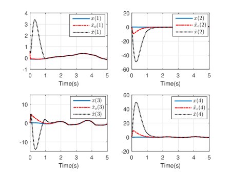
Figure 1: State variables, $x$, and their estimations using the proposed scheme, $\hat{x}_{o}$, and single sliding mode observer, $\hat{x}$, for $\mu=10^{2}$.

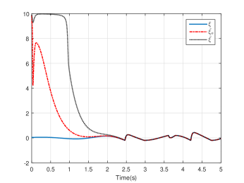
Figure 2: Fault signal, $\xi$, and its estimations using the proposed scheme, $\hat{\xi}_{o}$, and single sliding mode observer, $\hat{\xi}$, for $\mu=10^{2}$.

In order to demonstrate that choosing $\mu$ big enough results in a superior performance, the simulation is also performed for $\mu=10^{10}$. Fig. 3 and Fig. 4 show the obtained state and fault estimations for this value. The figures validate the theory and show that choosing $\mu$ results in a better performance in comparison to the conventional SMO.

V Conclusions

In this research a novel fault reconstruction scheme was presented using the concept of second level adaptation and SMOs. In the proposed scheme, the information provided by multiple SMOs with suitably chosen initial conditions was employed to reconstruct the system states and the fault (unknown input) rapidly. In this regard, it was shown that if the initial condition of system lies inside the convex hull of SMOs initial conditions, there exist some constant coefficients that provide a perfect state estimation. An estimation of these coefficients was obtained using the RLS algorithm. Mathematical analyses/justifications were provided to highlight performance of the proposed observation strategy. The stability of the overall system as well as the structure of the fault reconstruction scheme were fully addressed. Since the proposed approach employs the collective information obtained from multiple SMOs, it results in estimations with more preferable transient response in comparison to conventional SMO-based fault detection strategies.

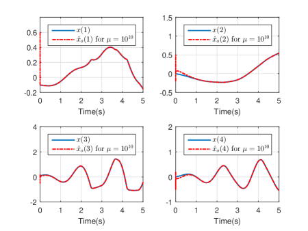
Figure 3: State variables, $x$, and their estimations using the proposed scheme, $\hat{x}_{o}$, for $\mu=10^{10}$.

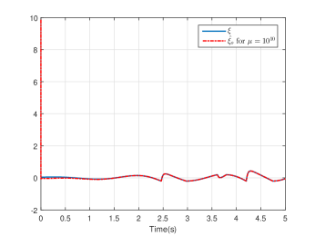
Figure 4: Fault signal, $\xi$, and its estimation using the proposed scheme, $\hat{\xi}_{o}$, for $\mu=10^{10}$.

References

- [1] S. Li, H. B. Sun, J. Yang, and X. H. Chen, “Disturbance-observer-based control and related methods-an overview,” IEEE Transactions on Industrial Electronics, vol. 63, no. 2, pp. 1083–1095, 2016.
- [2] S. Y. Lin, J. Y. Yen, M. S. Chen, S. H. Chang, and C. Y. Kao, “An adaptive unknown periodic input observer for discrete-time lti siso systems,” IEEE Transactions Automic Control, vol. 26, no. 8, pp. 4073–4079, 2017.
- [3] J. Zhang, P. Shi, and W. Lin, “Extended sliding mode observer based control for markovian jump linear systems with disturbances,” Automatica, vol. 70, pp. 140–147, 2017.
- [4] H. A. Talebi, K. Khorasani, and S. Tafazoli, “A recurrent neural-network-based sensor and actuator fault detection and isolation for nonlinear systems with application to the satellite’s attitude control subsystem,” IEEE Transactions Neural Networks, vol. 20, no. 1, pp. 45–60, 2009.
- [5] R. Salehi, G. Vossoughi, and A. Alasty, “A second-order sliding mode observer for fault detection and isolation of turbocharged si engines,” IEEE Transactions Industrial Electronics, vol. 62, no. 12, pp. 7795–7803, 2015.
- [6] M. Zhong, S. X. Ding, and D. Zhou, “A new scheme of fault detection for linear discrete time-varying systems,” IEEE Transactions Automatic Control, vol. 61, no. 9, pp. 2597–2602, 2016.
- [7] P. P. Menon and C. Edwards, “A sliding mode observer for monitoring and fault estimation in a network of dynamical systems,” International Journal of Robust and Nonlinear Control, vol. 24, pp. 2669–2685, 2014.
- [8] M. Navi, M. R. Davoodi, and N. Meskin, “Sensor fault detection and isolation of an industrial gas turbine using partial kernel pca,” IFAC-Papers OnLine, vol. 48, no. 21, pp. 1389–1396, 2015.
- [9] K. Esfandiari, F. Abdollahi, and H. A. Talebi, “Adaptive near-optimal neuro controller for continuous-time nonaffine nonlinear systems with constrained input,” Neural Networks, vol. 93, pp. 195–204, 2017.
- [10] G. David, “An introduction to observers,” IEEE Transactions Automatic Control, vol. 16, no. 6, pp. 596–602, 1971.
- [11] C. Edwards and S. Spurgeon, Sliding mode control: theory and applications. CRC Press, 1998.
- [12] K. Esfandiari, F. Abdollahi, and H. A. Talebi, “Adaptive output feedback tracking control for nonaffine nonlinear systems,” 2015 23rd Iranian Conference on Electrical Engineering, pp. 976–981, 2015.
- [13] K. Esfandiari, F. Abdollahi, and H. A. Talebi, “Stable adaptive output feedback controller for a class of uncertain non-linear systems,” IET Control Theory and Applications, vol. 9, no. 9, pp. 1329–1337, 2015.
- [14] H. Rios, J. Davila, L. Fridman, and C. Edwards, “Fault detection and isolation for nonlinear systems via high-order-sliding-mode multiple-observer,” International Journal of Robust and Nonlinear Control, vol. 25, pp. 2871–2893, 2015.
- [15] C. Edwards, S. K. Spurgeon, and R. J. Patton, “Sliding mode observers for fault detection and isolation,” Automatica, vol. 36, no. 4, pp. 541–553, 2000.
- [16] R. Galvan-Guerra, L. Fridman, and J. Davila, “High-order sliding-mode observer for linear time-varying systems with unknown inputs,” International Journal of Robust and Nonlinear Control, vol. 27, pp. 2338–2356, 2017.
- [17] C. P. Tan and C. Edwards, “Robust fault reconstruction in uncertain linear systems using multiple sliding mode observers in cascade,” IEEE Transactions on Automatic Control, vol. 55, no. 4, pp. 855–867, 2010.
- [18] F. N. Chowdhury and J. L. Aravena, “A modular methodology for fast fault detection and classification in power systems,” IEEE Transactions on Control Systems and Technology, vol. 16, no. 5, pp. 623–634, 1998.
- [19] H. Li, F. You, F. Wang, and S. Guan, “Robust fast adaptive fault estimation and tolerant control for t-s fuzzy systems with interval time-varying delay,” International Journal of Systems and Science, vol. 48, no. 8, pp. 1708–1730, 2017.
- [20] K. Zhang, B. Jiang, and P. Shi, “Fast fault estimation and accommodation for dynamical systems,” IET Control Theory and Applications, vol. 3, no. 2, pp. 189–199, 2009.
- [21] R. Postoyan, M. H. A. Hamid, and J. Daafouz, “A multi-observer approach for the state estimation of nonlinear systems,” in 54th IEEE Conference on Decision and Control (CDC), vol. 54th IEEE Conference on Decision and Control (CDC), 2015, pp. 1793–1798.
- [22] M. S. Chong, D. Nešić, R. Postoyan, and L. Kuhlmann, “Parameter and state estimation of nonlinear systems using a multi-observer under the supervisory framework,” IEEE Transactions on Automatic Control, vol. 60, no. 9, pp. 2336–2349, 2015.
- [23] Z. Han and K. S. Narendra, “New concepts in adaptive control using multiple models,” IEEE Transactions Automatic Control, vol. 57, no. 1, pp. 78–89, 2012.
- [24] W. Chen, J. Chen, and J. Sun, “A combination of second level adaptation and switching scheme for uncertain linear system,” in Control Conference (CCC), 2014 33rd Chinese.
- [25] K. S. Narendra and K. Esfandiari, “Adaptation in periodically varying environments using second level adaptation,” Technical Report, Yale University, arXiv preprint arXiv:, no. 1802, 2018.
- [26] K. S. Narendra and K. Esfandiari, “Adaptive control of linear periodic systems using multiple models,” 2018 IEEE Conference on Decision and Control (CDC), pp. 589–594, 2018.
- [27] V. K. Pandey, I. Kar, and C. Mahanta, “Adaptive control of nonlinear systems using multiple models with second-level adaptation,” in Systems Thinking Approach for Social Problems. Springer, 2015, pp. 239–252.
- [28] M. Shakarami, K. Esfandiari, A. A. Suratgar, and H. A. Talebi, “On the peaking attenuation and transient response improvement of high-gain observers,” 2018 IEEE Conference on Decision and Control (CDC), pp. 577–582, 2018.
- [29] V. K. Pandey, I. Kar, and C. Mahanta, “Control of twin-rotor mimo system using multiple models with second level adaptation,” IFAC-PapersOnLine, vol. 49, no. 1, pp. 676–681, 2016.
- [30] G. Bartolini, L. Fridman, A. Pisano, and E. Usai, “Modern sliding mode control theory: New perspectives and applications, volume 375 of lecture notes in control and information sciences,” 2008.
- [31] I. J. Bakelman, Convex analysis and nonlinear geometric elliptic equations. Springer Science & Business Media, 2012.
- [32] V. L. Hansen, Functional analysis: entering Hilbert space. World Scientific Publishing Co Inc, 2015.
- [33] C. Edwards and S. K. Spurgeon, “On the development of discontinuous observers,” International Journal of control, vol. 59, no. 5, pp. 1211–1229, 1994.
- [34] H. K. Khalil and J. Grizzle, Nonlinear systems. Prentice hall New Jersey, 1996, vol. 3.
- [35] V. I. Utkin, Sliding modes in control and optimization. Springer Science & Business Media, 2013.
- [36] A. Tamasevicius, “Hyperchaotic circuits: state of the art,” in Proc. 5th Int. Workshop Nonlinear Dynamics Electronic Systems (NDES’97), 1997, pp. 97–102.