The effect of tides on the Sculptor dwarf spheroidal galaxy

Abstract

Dwarf spheroidal galaxies (dSphs) appear to be some of the most dark matter dominated objects in the Universe. Their dynamical masses are commonly derived using the kinematics of stars under the assumption of equilibrium. However, these objects are satellites of massive galaxies (e.g. the Milky Way) and thus can be influenced by their tidal fields. We investigate the implication of the assumption of equilibrium focusing on the Sculptor dSph by means of ad-hoc $N$-body simulations tuned to reproduce the observed properties of Sculptor following the evolution along some observationally motivated orbits in the Milky Way gravitational field. For this purpose, we used state-of-the-art spectroscopic and photometric samples of Sculptor’s stars. We found that the stellar component of the simulated object is not directly influenced by the tidal field, while $\approx 30\%-60\%$ the mass of the more diffuse DM halo is stripped. We conclude that, considering the most recent estimate of the Sculptor proper motion, the system is not affected by the tides and the stellar kinematics represents a robust tracer of the internal dynamics. In the simulations that match the observed properties of Sculptor, the present-day dark-to-luminous mass ratio is $\approx 6$ within the stellar half-light radius ($\approx 0.3$ kpc) and $>50$ within the maximum radius of the analysed dataset ($\approx 1.5^{\circ}\approx 2$ kpc).

1 Introduction

Dwarf galaxies are the most numerous galaxies in the Universe (Ferguson & Binggeli, 1994): around the Local Group, about 70% of galaxies are dwarfs (McConnachie, 2012). The fraction remains this high also considering the Local Volume within 11 Mpc from the Milky Way (Dale et al., 2009). Understanding their structure, formation and evolution is a fundamental goal for astrophysics and cosmology (Klypin et al., 1999; Moore et al., 1999; Bullock et al., 2000; Grebel et al., 2003; Boylan-Kolchin et al., 2011; Mayer, 2011; Anderhalden et al., 2013; Battaglia et al., 2013; Walker, 2013; Read et al., 2017). Among them, the dwarf spheroidal galaxies (dSphs), satellites of the Milky Way, are close enough to measure the kinematics of individual stars (e.g.  Kleyna et al., 2002; Tolstoy et al., 2004; Battaglia et al., 2008; Muñoz et al., 2006a; Koch et al., 2007; Walker et al., 2009a; Massari et al., 2018). The analysis of kinematic dataset with equilibrium models leads to the finding that these galaxies are some of the most dark matter (DM) dominated object known to date (Mateo, 1998; Gilmore et al., 2007), with dynamical mass-to-light ratios up to several 100s (e.g. Mateo et al. 1993; Muñoz et al. 2006b; Battaglia et al. 2008; Koposov et al. 2011; Battaglia et al. 2011; see Mateo 1998 and Battaglia et al. 2013 for further information on the mass-to-light ratios of dSphs). Therefore, these objects are ideal laboratories to test theories on DM physics and cosmology (Navarro et al., 1996; Read et al., 2016; Macciò & Fontanot, 2010; Walker, 2013; Kennedy et al., 2014; Kubik et al., 2017).

However, since these dSphs are orbiting in the gravitational field of the MW, it is possible that the stellar tracers used to infer the dynamical state of these objects are influenced by tides and the assumption of equilibrium could introduce severe biases in the mass estimate (Kroupa, 1997; Fleck & Kuhn, 2003; Metz & Kroupa, 2007; Dabringhausen et al., 2016). For example, stars in undetected tidal tails (too faint or along the line-of-sight) could “pollute” the kinematic samples inflating the velocity dispersion, with a consequent overestimate the DM content, if inferred using equilibrium dynamical models (see e.g. Klimentowski et al., 2009; Read et al., 2006).

Several works have focused on the effects of the host gravitational field on the internal properties of dwarf galaxies by means of $N$-body simulations (e.g. Read et al., 2006; Peñarrubia et al., 2008, 2009a; Frings et al., 2017; Fattahi et al., 2018). The effect of tides on these galaxies strongly depends on their orbital history and the degree of pollution of tidally perturbed stars depends on the relative orientation of the internal part of the tides with respect to the line of sight. Therefore, the natural step forward is to perform similar analysis focusing on the properties of specific dSphs orbiting around the Milky Way. These works are based on $N$-body simulations tuned to reproduce the observed properties of the analysed dSph after their orbital evolution in the Milky Way tidal field. Works of this kind have been applied to Carina (Ural et al., 2015), Leo I (Sohn et al., 2007; Mateo et al., 2008), Fornax (Battaglia et al., 2015) and to the recently discovered Crater II (Sanders et al., 2018). However, one of the biggest source of uncertainty is the estimate of the proper motions that are indispensable to put the objects in realistic orbits to measure the actual effect of tides on the observables. The choice of a well-motivated orbit is essential to consider the right amount of tidal disturbance suffered by the dSphs and to rightly evaluate the degree of tidally perturbed stars contaminating the observed dataset. Luckily, at the moment we are living in the golden era of proper motion measurements thanks to the revolutionary Gaia DR2 catalogue (Gaia Collaboration et al., 2018a; Gaia Collaboration et al., 2018b; Fritz et al., 2018) and the very long baseline supplied by the HST measurements (e.g. Sohn et al., 2017).

Following the work of Battaglia et al. (2015), focused on the Fornax dwarf spheroidal, the aim of this paper is to investigate and quantify the effects of the tides on the structure and kinematics of the Sculptor dwarf spheroidal. Battaglia et al. (2015) found that in the case of Fornax tides have an almost negligible effect on the observed structure and kinematics of the stellar component, even considering the most eccentric orbits compatible with the observational constraints. Similarly to Fornax, the Sculptor dSph is one of the best studied Milky Way satellites (see e.g. Battaglia et al., 2008; Peñarrubia et al., 2009a; Walker et al., 2009b; Breddels & Helmi, 2014; Tolstoy, 2014; Strigari et al., 2018; Massari et al., 2018), so we can rely on high-quality spectroscopic data against which to compare our models (Walker et al., 2009a; Battaglia & Starkenburg, 2012). Moreover, the predicted Sculptor orbit is less external (smaller pericentre) than that of Fornax, so we expect that it could be more influenced by tides. For this aim, we ran a set of $N$-body simulations following the evolution of the structural and kinematic properties of Sculptor-like objects on orbits around the Milky Way that are consistent with the most recent observational constraints. Then, simulating “observations” in the last snapshot of the simulations, we investigated whether the observed kinematics of the stars is a robust tracer for the current dynamical state of Sculptor or the tides are introducing non-negligible biases.

The paper is organised as follows. In Sec. 2 we summarise Sculptor’s observational properties and we present a clean sample of Sculptor’s member stars that we use to analyse the kinematics and dynamics of Sculptor. In Sec. 3 we determine the possible Sculptor’s orbits around the Milky Way making use of the most recent and accurate Sculptor’s proper motion estimates. In Sec. 4, we use the information obtained in the previous sections to define a dynamical model of Sculptor compatible with the observable properties. Then, in Sec. 5 we describe the set-up of $N$-body simulations, whose results are presented in Sec. 6. Finally, in Sec. 7 we summarise and discuss the main results of this work.

2 Observed properties of the Sculptor dSph

2.1 Structure

Parameter	Value	Reference
($\ell$, $b$)	($287.53^{\circ}$, $-83.16^{\circ}$)	1
$D$	$86\pm 6^{\dagger}$ kpc	2
$L_{*}$	$2.3\times 10^{6}\ \,{\rm L}_{\odot}$	1
$\Upsilon_{*}$	$2$	3
$R_{\text{h}}$	$11.30\arcmin\pm 1.60\arcmin$ ($283\pm 45\ \,{\rm pc}^{\dagger}$)	1
$b_{*}$	$11.15\arcmin\pm 0.18\arcmin$ ($279\pm 4.5\ \,{\rm pc}^{\dagger}$)	C
$\epsilon$	$0.226\pm 0.014$	C
$PA$	$97.4^{\circ}\pm 1.2^{\circ}$	C
$V_{\text{sys}}$	$111.6\pm 0.2\ \,{\rm km\,s}^{-1}$	T
$\sigma_{\text{los}}(R<R_{\text{h}})$	$8.4\pm 0.2\ \,{\rm km\,s}^{-1}$	T
$\sigma_{\text{los}}(R<1.5^{\circ})$	$8.9\pm 0.2\ \,{\rm km\,s}^{-1}$	T

Table 1: Sculptor’s observational parameters. From the top to the bottom: Galactic coordinates ($\ell$,$b$), distance $D$, total luminosity in the $V$ band $L_{*}$, stellar mass-to-light ratio in the $V$ band $\Upsilon_{*}$, half-light radius $R_{\text{h}}$, best-fit Plummer scale length $b_{*}$, ellipticity $\epsilon$, position angle $PA$ (see Sec. 2.2); line-of-sight (los) systemic velocity $V_{\text{sys}}$, los velocity dispersion $\sigma_{\text{los}}$ estimated considering all the Sculptor’s stars within the half-light radius and $1.5^{\circ}$ (roughly the radial extent of our dataset, see Sec. 2.3.2). References: 1) McConnachie (2012); 2) Pietrzyński et al. (2008); 3) Mateo (1998); C) Cicuéndez, private communication; T) this work. $\dagger$Assuming the distance in the table the angular to physical scale conversion is $f_{\text{scale}}=25.02\pm 1.75\ \,{\rm pc}/\arcmin$.

The Sculptor dwarf spheroidal galaxy is a satellite of the Milky Way located close to the Galactic South Pole at Galactic coordinates ($\ell$, $b$)=($287.53^{\circ}$, $-83.16^{\circ}$). The distance to Sculptor has been measured with different methods: photometry of variable stars (RR Lyrae, e.g. Martínez-Vázquez et al. 2015; Miras, e.g. Menzies et al. 2011), of horizontal branch stars (e.g. Salaris et al. 2013), using the tip of the red giant branch (e.g. Rizzi et al. 2007) and analysing the colour magnitude diagram of the stars in the galaxy (e.g. Weisz et al. 2014). We decided to take as a reference the value $D=86\pm 6\ \,{\rm km\,s}^{-1}$, adopting the distance modulus obtained by Pietrzyński et al. (2008) using the near-infrared photometry ($J$ and $K$ bands) of a sample of 76 RR Lyrae stars. This value is compatible with the recent estimate by Garofalo et al. (2018).

There is evidence that Sculptor contains two distinct distinct stellar populations: a more concentrated metal rich population with low velocity dispersion ($\approx 6-7\ \,{\rm km\,s}^{-1}$) and a more extended metal poor population with high velocity dispersion ($\approx 10-12\ \,{\rm km\,s}^{-1}$); see e.g. Tolstoy et al. (2004); Battaglia et al. (2008); Walker & Peñarrubia (2011). As well known, the existence of two populations can be exploited to constrain the mass distribution of the galaxy (e.g. Battaglia et al. 2008; Amorisco & Evans 2012; Walker & Peñarrubia 2011; Strigari et al. 2017). However, since the purpose of this work is not a detailed study of the internal dynamics of Sculptor, we assume for simplicity the presence of a single stellar component. We discuss the possible implications of this assumption in Sec. 7.

The properties of the light distribution have been derived employing the same state-of-the-art technique used by Cicuéndez et al. (2018) for the Sextans dwarf spheroidal applying it on a publicly available VST/ATLAS $g$-band and $r$-band photometric catalogue of stellar sources covering $\approx$ 4 deg² on the line of sight to Sculptor (Cicuéndez, private communication). The best-fit (constant) ellipticity is $\epsilon=0.226\pm 0.014$ (axial ratio $q\approxeq 0.77$) and the best fit position angle is $PA=97.4^{\circ}\pm 1.2^{\circ}$, in agreement with the values of Battaglia et al. (2008). The best fit to the observed surface number-density profile is a (projected) Plummer profile

$$N_{*}\propto\left(1+\frac{R^{2}_{\text{ell}}}{b^{2}_{*}}\right)^{-2},$$ (1)

where $R_{\text{ell}}$ is the elliptical radius corresponding the to major axis of the elliptical iso-density contours and the best fit scale length is $b_{*}=11.15\arcmin\pm 0.18\arcmin=279\pm 5\ \text{pc}$. The main observed properties of Sculptor are summarised in Tab. 1.

2.2 Proper motions

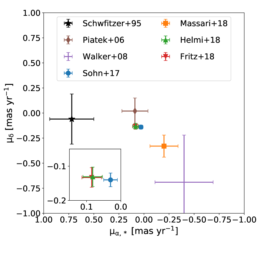
Figure 1: Sculptor’s proper motion estimates: Schweitzer et al. (1995) (black star), Piatek et al. (2006) (brown diamond), Walker et al. (2008) (violet cross), Walker & Peñarrubia (2011) (pink pentagon), Sohn et al. (2017) (blue dot), Massari et al. (2018) (orange square), Gaia Collaboration et al. (2018b) (green up-triangle), Fritz et al. (2018) (red down-triangle). The inset shows a zoom-in in the region around the recent Gaia DR2 proper motion estimates. Note that $\mu_{\alpha,*}=\mu_{\alpha}\cos\delta$.

There are several direct estimates of the systemic proper motion of Sculptor from astrometric measurements (Schweitzer et al., 1995; Piatek et al., 2006; Sohn et al., 2017; Massari et al., 2018; Gaia Collaboration et al., 2018b; Fritz et al., 2018) and indirect estimates by Walker et al. (2008); Walker & Peñarrubia (2011) using the apparent velocity gradient along the direction of the proper motion. The currently available estimates of the Sculptor’s proper motion are summarised in Fig. 1. While the first measurements were quite uncertain and not all in agreement among each other, in the last couple of years the long time baseline of the HST data and the high-quality astrometric data from Gaia (Gaia Collaboration et al., 2016; Gaia Collaboration et al., 2018a) have drastically improved the proper motion estimate for Sculptor. In particular, those obtained using the Gaia DR2 astrometry (Gaia Collaboration et al. 2018b; Fritz et al. 2018) and the one obtained from the HST with a $\approx 11$ yr long baseline (Sohn et al., 2017) converge toward a likely “definitive” value. In the rest of the paper we consider only the four most recent estimates: Sohn et al. (2017) (S17), Massari et al. (2018) (M18), Gaia Collaboration et al. (2018b) (H18) and Fritz et al. (2018) (F18). We assumed the errors for the H18 and F18 proper motions (see Fig. 1 and Tab. 3.1) as the quadratic sum of the nominal errors reported in the corresponding papers and the Gaia DR2 proper motions systematic error $\delta\mu_{\text{s}}\approx 0.028\ \text{mas}\ \text{yr}^{-1}$. This last value has been estimated from Eq. 18 in Gaia Collaboration et al. (2018a) considering a spatial scale of $1^{\circ}$ roughly corresponding to the extension of the bulk of the Gaia DR2 Sculptor’s member analysed in H18 (see Sec. 7 for a discussion about the assumed systematic errors). Considering the older proper motion estimates it is interesting to compare the two non-astrometric measurements (Walker et al., 2008; Walker & Peñarrubia, 2011) with the most recent ones. In these older works the Sculptor’s proper motion was estimated assuming that any possible line-of-sight velocity gradient is entirely caused by the relative motion between Sculptor and the Sun (see Sec. 2.3.3). However, if a significant intrinsic rotation is present, the results of this analysis can be heavily biased. Therefore, a significant difference with respect to the astrometric proper motion measurements could be an indication of an intrinsic rotation. We found that the non-astrometric measurement are consistent within $\approx 1\sigma$ with M18 and within $\approx 2\sigma$ with S17, H18 and F18. Even if the differences are not significant, we note that these results are mainly driven by the large errors reported in Walker et al. (2008); Walker & Peñarrubia (2011). Hence, a strong claim in favour or against the presence of intrinsic rotation cannot be made from a simple comparison of astrometric and non-astrometric proper motion measurements.

2.3 Internal kinematics

2.3.1 The sample

We derive the line-of-sight (los) velocity dispersion profile of Sculptor using a state-of-the-art dataset obtained combining the MAGELLAN/MIKE catalogue presented in Walker et al. (2009a) (1541 stars, W09 hereafter) and the VLT/FLAMES-GIRAFFE catalogue Battaglia & Starkenburg (2012) (1073 star, BS12 hereafter). The BS12 catalogue contains stars from the original catalogues by Tolstoy et al. (2004), Battaglia et al. (2008) and Starkenburg et al. (2010).

2.3.2 Member selection

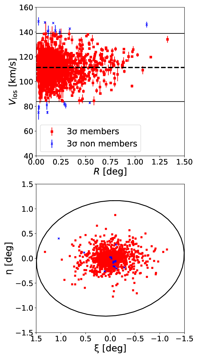
Figure 2: Sculptor’s member selection. Sculptor’s members and contaminants (likely unresolved binaries) are shown as red squares and blue x-crosses, respectively. Top panel: line-of-sight velocity, $\,{V}_{\rm los}$, versus circular projected radius, $R$; the horizontal lines denote the mean systemic velocity $\,{V}_{\rm sys}$ (dashed) of Sculptor and the $\pm 3\sigma$ region (solid). Bottom panel: position of the stars with respect to the Sculptor centre ($\xi$ and $\eta$ represent the gnomonic projection of the Galactic sky coordinates); the ellipse is centred on the Sculptor centre: it has a major axis $a=1.5^{\circ}$, ellipticity $\epsilon=0.226$ and position angle $PA=97.4^{\circ}$ (see Sec. 2.1 and Tab. 1).

The two catalogues contain both genuine Sculptor’s members and Milky Way interlopers. To start with, for the stars in BS12, we applied the cleaning of contaminants using the equivalent width of the Mg I line at $8806.8$ Å as described in BS12. For the stars in W09, we removed all the objects with a member probability lower than 0.5 (see W09 for details on the Sculptor’s member probability estimate). Then, we cross-matched the spectroscopic sample with the Gaia DR2 catalogue (Gaia Collaboration et al., 2018a) to complement it with proper motion and parallax estimates. We removed all the stars that are not compatible with the H18 Sculptor proper motion and with zero parallax within three times the error. For the parallax, the error corresponds to the uncertainty on the individual parallax measurement; for the proper motion the error is a quadratic sum of the uncertainty in the individual measurement, the error on the systemic proper motion and the systematic error of 0.028 mas/yr (see Lindegren et al., 2018, see also Sec. 2.2). Finally, we removed all the stars with los velocities $V_{\rm los}$ differing at least by $50\ \,{\rm km\,s}^{-1}$ from $111\ \,{\rm km\,s}^{-1}$ (roughly the Sculptor systemic velocity). After the selection cuts, we are left with 540 stars from BS12 and 1312 stars from W09.

In order to identify and analyse duplicate objects, we cross-matched the two catalogues considering a search-window of $1\arcsec$ and we found 276 duplicated stars. For each of them we estimate the velocity difference $\Delta V_{\rm los}=V_{\rm los,BS12}-V_{\rm los,W09}$ and the related uncertain $\delta\Delta V_{\rm los}=\sqrt{\delta V^{2}_{\rm los,BS12}+\delta V^{2}_{\rm los,W09}}$. We considered that all the stars with $|\Delta V_{\rm los}/\delta\Delta V_{\rm los}|>3$ are unresolved binary systems and we filtered them out from the two catalogues. Among the duplicated stars, only 17 have been removed, resulting in a $6\%$ fraction of unresolved binaries. Considering the los velocity distribution of the 259 remaining stars, we found and correct a velocity offset of $\simeq-1\,{\rm km\,s}^{-1}$ of the stars in BS12 with respect the stars in W09. Finally, these stars are combined in a single dataset estimating the $V_{\rm los}$ as the error-weighted mean of the single velocity measurements.

The joined Sculptor’s stars catalogue contains 1559 stars ($\approx 66\%$ from W09, $\approx 17\%$ from BS12 and $\approx 17\%$ from both catalogues). As a final conservative cleaning criterion, we applied an iterative $3\sigma$ clipping removing 16 stars with large deviation from the systemic velocity. Fig. 2 shows that most of these stars are located in the central part of Sculptor, hence it is unlikely that they are Milky Way contaminants survived to the selection cuts. Rather, we considered these stars (with single observations in BS12 or W09) as likely unresolved binaries. The fraction of the removed objects ($\approx 1\%$) is roughly compatible with the binary fraction estimated analysing the stars duplicated among the two catalogues. We stress that the $\sigma$ clipping method used to filter binary systems is capable to select only short-period binaries (few days; see Minor 2013; Spencer et al. 2018) for which the typical orbital velocities are significantly higher than the los velocity errors ( $\langle\delta V_{\text{los}}\rangle\approx 2\ \,{\rm km\,s}^{-1}$) and/or than the dwarf velocity dispersion ($\sigma_{\text{los}}\approx 9\,{\rm km\,s}^{-1}$, see Fig. 3). Given the expected distribution of binary periods (Duquennoy & Mayor, 1991; Minor, 2013), the short-period systems represent only a tiny fraction of the binaries. Therefore, our estimated binary fraction represents a strong lower limit (Minor 2013 estimated a 0.6 binary fraction for Sculptor). However, even if most of the stars in our final sample are in fact part of binary systems, their expected radial velocities due to the orbital motions are smaller or compatible with the velocity errors and much smaller than the intrinsic velocity dispersion of the system. Therefore, the kinematic bias introduced by the binary stars on the estimate of the velocity dispersion profile (Sec. 2.3.3) and on the dynamical mass (Sec. 4.2) is negligible (see e.g. Hargreaves et al., 1996; Olszewski et al., 1996).

The final catalogue contains 1543 objects. The systemic velocity of Sculptor, estimated as the mean velocity of its members, is $V_{\rm sys}=111.6\ \pm 0.2\ \,{\rm km\,s}^{-1}$; the velocity dispersion is $\sigma_{\text{los}}=8.9\ \pm 0.2\ \,{\rm km\,s}^{-1}$ considering the whole catalogue and $\sigma_{\text{los}}=8.4\ \pm 0.2\ \,{\rm km\,s}^{-1}$ considering only stars within the half-light radius. The errors on these values have been estimated using the bootstrap technique (Feigelson & Babu, 2012).

2.3.3 Velocity dispersion profile

The relative motion of Sculptor with respect to the Sun causes an artificial los velocity gradient along the proper motion direction (see e.g.  Walker et al., 2008). Therefore, we corrected the measured los velocity for this perspective effect through the methodology described in the Appendix A of Walker et al. (2008) using the systemic proper motion estimated in H18 and the systemic los velocity reported in Tab. 1. The errors on the corrected $V_{\text{los}}$ have been estimated with a Monte Carlo simulation considering the observational uncertainties on $V_{\text{los}}$, the errors on $V_{\text{sys}}$ and distance (Tab. 1), and the error on the proper motions (Tab. 3.1).

The radial profile of los velocity dispersion $\sigma_{\text{los}}(R)$, has been obtained grouping Sculptor’s members in (circular) radial bins. In order to have the best compromise between good statistics and spatial resolution (bin width), we decided to select the bin edges so that each bin contains 150 stars. Since the outermost bin remains with 41 stars only, we merged it with the adjacent bin, obtaining a wider outermost bin with 192 stars. For each of the final 10 bins, we estimated the mean los velocity $\overline{V}_{\text{los}}$ and the velocity dispersion $\sigma_{\text{los}}$ fitting a Gaussian model and taking into account the $V_{\text{los}}$ uncertainties through an extreme-deconvolution technique (Bovy et al., 2011). Similarly, we estimated the representative radius of each bin taking the mean of the circular radius of the stars. The errors on these values have been estimated using the bootstrap technique (Feigelson & Babu, 2012). The resultant $\sigma_{\text{los}}(R)$ profile is shown and compared with the profiles from Walker et al. (2009b) and Breddels & Helmi (2013) in Fig. 3. The two profiles are compatible with our profile within the half-light radius. Beyond this radius the $\sigma_{\text{los}}$ estimated in this work are systematically lower with respect to the values of Breddels & Helmi (2013), but compatible with the Walker et al. (2009b) estimates. This discrepancy is not due to the predominance of stars from W09 in our joined catalogue (see Sec. 2.3.2), because the two outermost bins are dominated by stars taken from BS12 (see bottom bars in Fig. 3). The most likely explanation is that the velocity dispersion profile reported in Breddels & Helmi (2013) is slightly inflated by residual Milky Way interlopers.

The assumptions we made to obtain the final binned profile are discussed below.

• $N_{\text{star}}$ per bin. We repeated the analysis described above changing the number of stars per bin from 100 to 350 in steps of 50. The increase of the number of stars per bin reduces the errors in $\sigma_{\text{los}}$ but it decreases the spatial resolution. The final profiles are all compatible, but the chosen value of 150 represents the best compromise between the two kinds of uncertainties.

• Velocity gradient. The correction for the perspective velocity gradient due to the relative motion between the Sun and Sculptor has been applied using the H18 proper motion. We repeated the correction procedure considering also the M18 and S17 proper motions. The differences on the final velocity dispersion profiles are negligible ($<1\%$). Even if some residual shallow velocity gradient should still be present, e.g. due to an intrinsic rotational motion (e.g. Battaglia et al. 2008, see also Sec. 2.2; Zhu et al. 2016, see also Sec. 2.2), any possible bias in the velocity dispersion should be important only in the outermost bins where the ratio between the velocity dispersion and the rotation velocity is larger. Considering as a test a rotation velocity of $7\ \,{\rm km\,s}^{-1}$ and a velocity dispersion of $10\ \,{\rm km\,s}^{-1}$ and a sample of 150 stars uniformly distributed along the azimuthal angle, we found that the increase of the velocity dispersion is expected to be lower than $10\%$. This value is “safely” within the error bars of the outermost points of the estimated velocity dispersion profile.

• Circular vs elliptical bins. We estimated new velocity dispersion profiles as a function of the elliptical radius $R_{\text{ell}}=\sqrt{x^{2}+y^{2}/q^{2}}$ and of the circularised radius $R_{\text{circ}}=\sqrt{x^{2}q+y^{2}/q}$, where $q$ is the observed Sculptor’s axial ratio (see Sec. 2.1) and $(x,y)$ are the Cartesian coordinates in the reference aligned with the Sculptor’s principal axes. The $\sigma_{\text{los}}(R_{\text{ell}})$ and $\sigma_{\text{los}}(R_{\text{circ}})$ profiles are practically coincident and both the normalisation and the radial trend are compatible with the los velocity dispersion profile shown in Fig. 3.

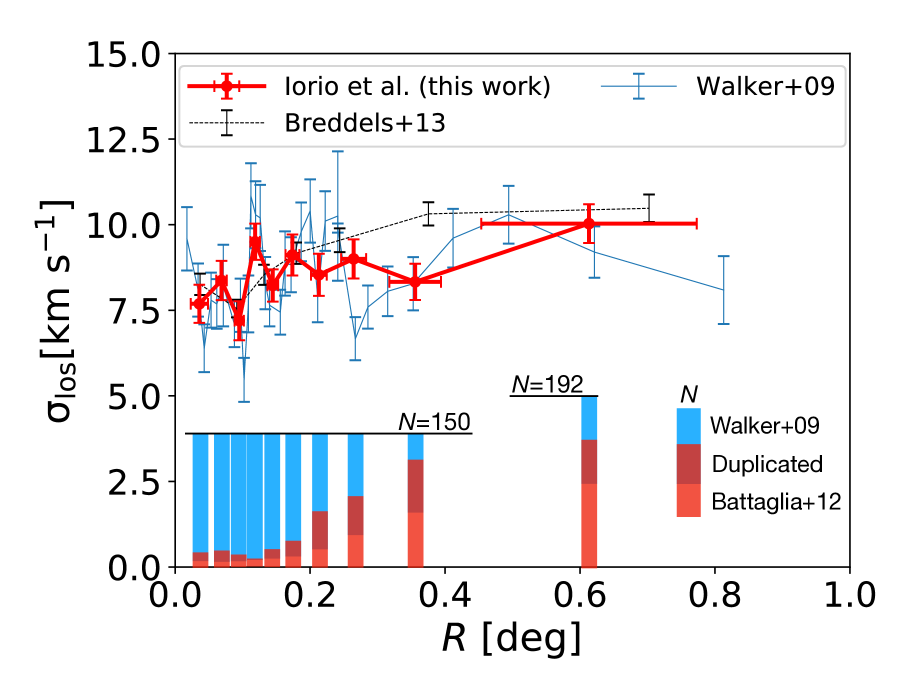
Figure 3: Velocity dispersion profile of Sculptor: this work (red points and line), Walker et al. (2009b) (blue line), Breddels & Helmi (2013) (black dashed line). The histograms in the bottom part of the plot indicate the fraction of stars in each bin belonging to the original samples of W09 (blue bars) and of BS12 (red bars). The dark-red areas, coming from the intersection of the blue and red bars, represent the fraction of common stars between the two samples (see Sec. 2.3.2). All bins have 150 stars, but the outermost bin that has 192 stars. See the text for the detailed description of our binning technique.

We stress that the aim of this paper is not the detailed study of the velocity dispersion profile in Sculptor, but rather we want to have a self-consistent way to infer the velocity dispersion profile both in observations and in simulations. The performed analysis and the comparison of our profile with results in the literature (Fig. 3) ensures that our “simple” technique and our assumptions do not cause severe biases in the final estimate of $\sigma_{\text{los}}$.

3 The orbit of Sculptor

3.1 Milky Way model

			Milky Way model
	Proper motions		B14		J95
Model	$\mu_{\alpha,*}$ ($\text{mas}\ \text{yr}^{-1}$) (1a)	$\mu_{\delta}$ ($\text{mas}\ \text{yr}^{-1}$) (1b)	$\,{r}_{\rm apo}$ [kpc] (2a)	$\,{r}_{\rm peri}$ [kpc] (2b)	$\,{r}_{\rm apo}$ [kpc] (3a)	$\,{r}_{\rm peri}$ [kpc] (3b)
[HTML]CCCCCC    [HTML]CCCCCCH18		$0.082\pm 0.028^{\dagger}$	$-0.131\pm 0.028^{\dagger}$	$145^{+17}_{-23}$ $[99,246]$	$65^{+6}_{-7}$ $[45,83]$	$105^{+8}_{-7}$ $[84,132]$	$54^{+6}_{-4}$ $[36,74]$
F18	$0.085\pm 0.029^{\dagger}$	$-0.133\pm 0.029^{\dagger}$	$143^{+17}_{-22}$ $[99,244]$	$64^{+6}_{-6}$ $[45,83]$	$105^{+7}_{-8}$ $[83,130]$	$54^{+6}_{-7}$ $[36,74]$
[HTML]CCCCCC    [HTML]CCCCCCM18		$-0.200\pm 0.140$	$-0.330\pm 0.110$	$361^{+425}_{-273}$ $[81,2428]$	$81^{+7}_{-9}$ $[21,101]$	$141^{+49}_{-55}$ $[73,811]$	$78^{+11}_{-11}$ $[18,101]$
S17	$0.030\pm 0.020$	$-0.140\pm 0.020$	$152^{+17}_{-21}$ $[111,266]$	$67^{+5}_{-11}$ $[54,85]$	$108^{+8}_{-8}$ $[87,135]$	$60^{+5}_{-6}$ $[45,76]$

Table 2: Orbital parameters estimated for different proper motions of Sculptor: H18, F18, M18 and S17 (Cols. 1a/1b). For each of them, we integrated $10^{5}$ orbits varying all the Sculptor (Tab. 1) and Milky Way parameters accordingly with their errors (see the text). The columns report the statistics of the posterior distributions obtained for the radius of the apocentre (Cols. 2a/3a) and of the pericentre (Cols. 2b/3b) assuming the Milky Way models B14 and J95. The numbers indicate the values obtained considering the fiducial value for the Sculptor and Milky Way parameters, the superscript and the subscript represent the interval that contains the $68\%$ ($1\sigma$) of the distribution. The values inside the square brackets indicate the interval containing the $99.7\%$ ($3\sigma$) of the distribution. $\dagger$The errors are the quadratic sum of the nominal errors reported in H18 and F18 and the $0.028\ \text{mas}\ \text{yr}^{-1}$ Gaia systematic error (Lindegren et al., 2018).

Despite a large number of studies focusing on the Milky Way dynamics, the detailed gravitational potential of the Galaxy is still far from being nailed down. Although there is convergence in the mass estimate in the inner part of the DM halo ($r\lesssim 50\$ kpc, e.g. Wilkinson & Evans, 1999; Xue et al., 2008; Deason et al., 2012; Gibbons et al., 2014), results of different works predict a relative wide range of values for the Galactic virial mass $M_{200}$ (Wang et al., 2015, and reference therein). We can roughly divide the different results in three groups: works predicting a “heavy” Milky Way with $M_{\text{200}}\gtrsim 2\times 10^{12}\ \,{\rm M}_{\odot}$ (e.g. Li & White, 2008), works predicting a “light” Milky Way with $M_{\text{200}}\lesssim 1\times 10^{12}\ \,{\rm M}_{\odot}$ (e.g. Battaglia et al., 2005; Gibbons et al., 2014) and other works in between with $M_{\text{200}}\approx 1.2-1.8\times 10^{12}\ \,{\rm M}_{\odot}$ (e.g. Piffl et al., 2014, see also recent estimates by Contigiani et al. 2018; Monari et al. 2018; Posti & Helmi 2018).

In this work we considered two “extreme” analytical Milky Way dynamical models: the “heavy” model by Johnston et al. (1995, J95), and the “light” model by Bovy (2014, B14). We decided to investigate the orbital properties of Sculptor both in the J95 and B14 potentials. The J95 model consists in a Miyamoto-Nagai disk (Miyamoto & Nagai, 1975) with mass $M=10^{11}\ \,{\rm M}_{\odot}$, a spherical Hernquist bulge (Hernquist, 1990) with mass $M=3.40\times 10^{10}\ \,{\rm M}_{\odot}$ and a spherical logarithmic dark halo. The B14 model includes a Miyamoto-Nagai disk with mass $M=6.80\times 10^{10}\ \,{\rm M}_{\odot}$, a spherical bulge with a truncated power-law density profile with mass $M=0.45\times 10^{10}\ \,{\rm M}_{\odot}$ and a spherical Navarro-Frenk-White (NFW; Navarro et al. 1996) dark halo. The mass profile in J95 rises from $\simeq 0.5\times 10^{12}\ \,{\rm M}_{\odot}$ at $50\ \,{\rm kpc}$ to $\simeq 2.3\times 10^{12}\ \,{\rm M}_{\odot}$ at $300\ \,{\rm kpc}$. In the same radial range the mass in B14 increases from $\simeq 0.3\times 10^{12}\ \,{\rm M}_{\odot}$ to $\simeq 1.0\times 10^{12}\ \,{\rm M}_{\odot}$.

We set a left-handed Cartesian reference frame $(x_{\text{g}},y_{\text{g}},z_{\text{g}})$ centred in the Galactic centre and such that the Galactic disc lies in the $x_{\text{g}}$-$y_{\text{g}}$ plane, the Sun lies on the positive $x$-axis and the Sun rotation velocity is $\dot{y}_{\text{g}}>0$. In this frame of reference, the Sun is at a distance of $R_{\odot}=8.0\pm 0.5$ kpc (Bovy et al., 2012) from the Galactic centre and the rotational velocity of the local standard of rest (lsr) is $V_{\text{lsr}}=218.0\pm 6.0\ \,{\rm km\,s}^{-1}$ (Bovy et al., 2012). Finally, we used the estimate of the solar proper motion with respect to the lsr reported in Schönrich (2012): ($U_{\odot},\ V_{\odot},\ W_{\odot}$)=($-11.1\pm 1.3,\ 12.2\pm 2.1,\ 7.25\pm 0.6$) $\,{\rm km\,s}^{-1}$. Therefore, the motion of the Sun in the Galactic frame of reference is $\vec{\upsilon}_{\odot}=(U_{\odot},\ V_{\odot}+V_{\text{lsr}},\ W_{\odot})$. The estimated solar motion ($\vec{\upsilon}_{\odot}$) is used in Sec. 3.2 to obtain the velocity of Sculptor in the Galactocentric frame of reference from the observed kinematics (proper motions and los velocity).

3.2 Orbital parameters

We used the leapfrog orbit integrator in the Python module galpy (Bovy, 2015) to investigate the orbits of Sculptor. Combining the the proper motion estimates (H18, F18, M18 and S17, see Sec. 2.2) and the two Milky Way potentials (J95 and B14; see Sec. 3.1) we consider 8 families of orbits. For each family, we performed $10^{5}$ orbit integrations drawing the values of the proper motions, the Sculptor systemic velocity, the Sculptor distance, the Sun position and motion in the Galactic frame of reference from Gaussian distributions centred on the measured values and with dispersion given by the corresponding errors. In the case of H18 and F18, we took into account the reported proper motion correlation extracting the values of $\mu_{\alpha,*}$ and $\mu_{\delta}$ from a bidimensional normal distribution. Each orbit has been integrated backward from the present-day position of Sculptor for $8$ Gyr. The chosen integration time represents a good compromise between a time long enough to explore the effect of tides and a time window in which the mass evolution of the Milky Way can be considered almost negligible. In particular, we notice that the last significant Milky Way merger likely happened 8-11 Gyr ago (Belokurov et al., 2018; Myeong et al., 2018; Helmi et al., 2018; Kruijssen et al., 2018).

The final apocentre and pericentre distributions for each of the 8 investigated families of orbits are summarised in Tab. 3.1. The H18, F18 and S17 proper motion estimates give very similar results, largely compatible within the error. As expected the orbits in the “light” Milky Way potential (B14) have both larger apocentre and pericentre with respect to the case of the “heavy” Milky Way model (J95). The results obtained for M18 using the fiducial proper motion values are slightly offset towards more external orbits, however given the larger proper motion errors, the overall results are still compatible with the other estimates. It is worth noting that the pericentres found assuming the H18, F18 and S17 proper motions are consistent with the first estimate of the Sculptor’s pericentre, $\,{r}_{\rm peri}=68\ \,{\rm kpc}$, obtained by Piatek et al. (2006).

	$R_{\odot}$ [kpc] (1)	$\vec{v}_{\odot}$ $(V_{x},V_{y},V_{z})$ [$\,{\rm km\,s}^{-1}$] (2)	$V_{\text{sys}}$ [$\,{\rm km\,s}^{-1}$] (3)	$D$ [kpc] (4)	$\vec{\mu}$ $(\mu_{\alpha,*},\mu_{\delta})$ [$\text{mas}\ \text{yr}^{-1}$] (5)
FH18	$8.0$	$(-11.1,230.2,7.3)$	$111.6$	$86.0$	$(0.085,-0.133)$
EH18	$8.2$	$(-10.9,213.3,7.9)$	$111.8$	$82.3$	$(0.125,-0.164)$

Table 3: Parameters that give rise to the two orbits used in the $N$-body simulations. (1) distance of the Sun from the Galactic centre; (2) proper motion of the Sun in the Galactic frame of reference (see text); (3) Sculptor’s los systemic velocity; (4) Sculptor’s distance from the Sun; (5) Sculptor’s proper motion.

Given the similarity of the orbital properties, we decided, without loss of generality, to consider the distribution of orbital parameters obtained with the H18 proper motions as our reference to set up of $N$-body simulations. Moreover, since we are interested in the influence of Milky Way tidal field on the observed properties of Sculptor, we make the conservative choice to consider in the simulations the J95 Milky Way potential model. If no strong tidal effects are found using this potential, it is likely that we can safely extend this result to any other realistic axisymmetric Milky Way potential model.

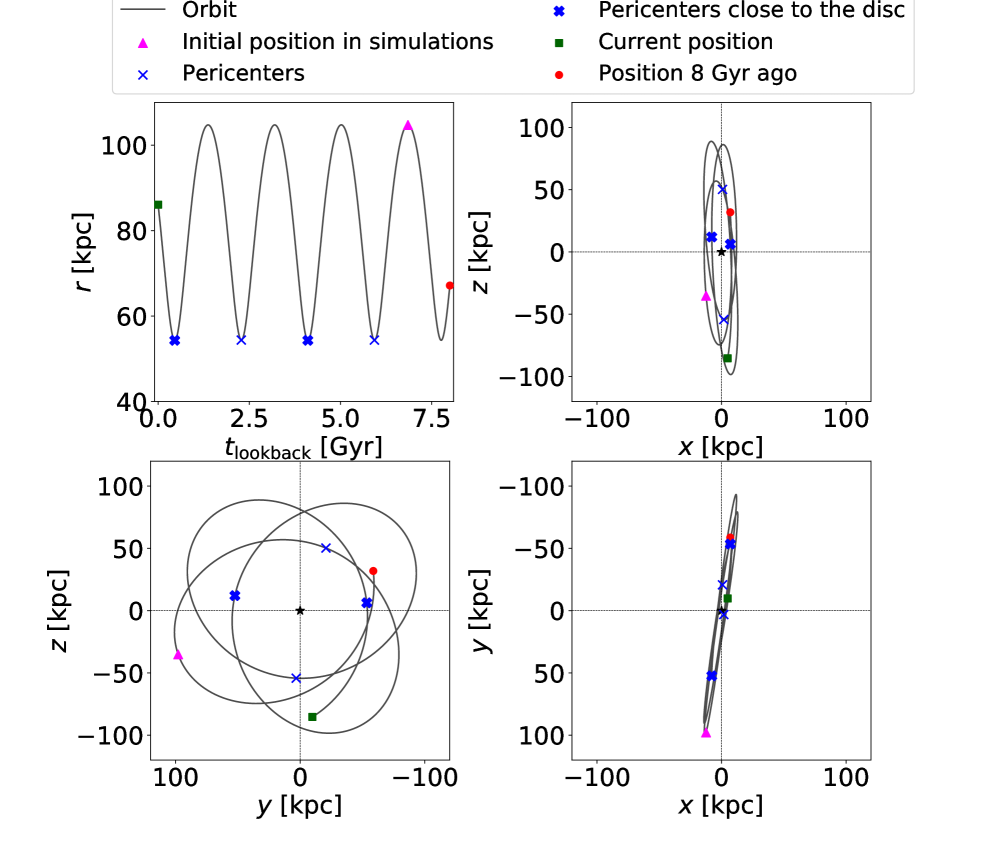
Figure 4: FH18 orbit of Sculptor (see Tab. 3) integrated backward for 8 Gyr from the present position (green square). The $(x,y,z)$ Galactocentric frame of reference is defined in Sec. 3.1 and $r=\sqrt{x^{2}+y^{2}+z^{2}}$ is the Galactocentric radius. The lookback time $t_{\text{lookback}}$ indicates the time in the past considering the backward orbit integration. The red circle is the position at the end of the orbit integration. The magenta triangles indicate the starting location of Sculptor in the $N$-body simulation (see Sec. 5.2.2). The blue crosses indicate the positions of the pericentres, the thicker crosses highlight the pericentres located close to the Galactic plane ($z<20\ \,{\rm kpc}$). The black stars indicate the Galactic centre.

In the $N$-body simulations (Sec. 5) we consider two different orbits. The first, labelled FH18, has been obtained using the fiducial values of all the Sculptor and Milky Way parameters reported in Tab. 1, Tab. 3.1 and Sec. 3.1. The second, labelled EH18, is the orbit that, among all the $10^{5}$ realisations, has the pericentric radius closest to the left $3\sigma$ extreme of the pericentre distribution. The FH18 orbit has pericentre $\,{r}_{\rm peri}=54\ \,{\rm kpc}$, apocentre $\,{r}_{\rm apo}=105\ \,{\rm kpc}$, eccentricity $e=0.32$, and radial orbital period $T=1.6\ \text{Gyr}$. In the EH18 case, the orbit has pericentre $\,{r}_{\rm peri}=36\ \,{\rm kpc}$, apocentre $\,{r}_{\rm apo}=94\ \,{\rm kpc}$, eccentricity $e=0.44$, and radial orbital period $T=1.3\ \text{Gyr}$. The projections of the FH18 and EH18 orbits in the Galactic planes are shown in Fig. 4 and Fig. 5, respectively. In both the FH18 and EH18 orbits Sculptor is currently heading towards its next apocentre after the last pericentric passage ($\approx 0.5\ \text{Gyr}$ ago). The parameters that give rise to the orbits FH18, EH18 and EM18 are summarised in Tab. 3.

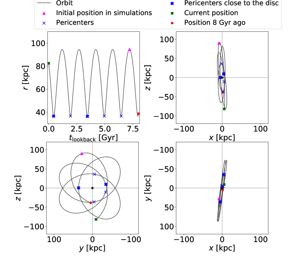
Figure 5: Same as Fig. 4 bur for the EH18 orbit (see Tab. 3).

4 Dynamical models of Sculptor

In order to set up the initial conditions of the $N$-body simulations (Sec. 5) we have to define a density model for both the DM halo and the stellar component of Sculptor. As a startig point, in the present section we construct spherically symmetric equilibrium dynamical models that represent Sculptor as it is observed today.

4.1 Density distributions

4.1.1 Stars

Based on the observed light distribution of Sculptor (see Sec. 2.1), we used a 3D Plummer profile to model the density law for the stellar component,

$$\rho_{*}(r)=\rho_{0}\left(1+\frac{r^{2}}{b^{2}_{\text{*}}}\right)^{-2.5}.$$ (2)

In Eq. 2 the angular length of the Plummer core radius, $b_{*}=11.15\arcmin$, is set from the fit to the observed light profile of Sculptor (Sec. 2.1) and the physical length depends on the assumed distance that can vary in different orbits (see Tab. 3). Thus $b_{*}=0.279\ \,{\rm kpc}$ for the FH18 orbit ($D=86.0$ kpc) and $b_{*}=0.267\ \,{\rm kpc}$ for the EH18 orbit ($D=82.3$ kpc). The normalisation factor is

$$\rho_{0}=M_{*}\frac{3}{4\pi b^{3}_{*}}\left(\frac{b^{2}_{*}+R^{2}_{*}}{R^{2}_{*}}\right),$$ (3)

where $R_{*}=1.5^{\circ}\simeq 8b_{*}$ ($\approx 2.2\ \,{\rm kpc}$ and $\approx 2.1\ \,{\rm kpc}$ for FH18 and EH18 orbits respectively) is a reference (projected) radius that is equal to the length of the major axis of the ellipse containing all the stars in our sample (see Fig. 2). Given the Plummer surface density profile

$$\Sigma_{*}(R)=\rho_{0}\int^{\infty}_{R}\text{d}r\left(1+\frac{r^{2}}{b^{2}_{\text{*}}}\right)^{-2.5}\frac{r}{\sqrt{r^{2}-R^{2}}}=\Sigma_{0}\left(1+\frac{R^{2}}{b^{2}_{*}}\right)^{-2},$$ (4)

the value of the parameter $\rho_{0}$ introduced in Eq. 3 is fixed by the condition $2\pi\int_{0}^{R_{*}}\Sigma_{*}(R)R\text{d}R=M_{*}$, where $M_{*}=\Upsilon_{*}L_{*}=4.6\times 10^{6}\ \,{\rm M}_{\odot}$ and $L_{*}=2.3\times 10^{6}$ is the total luminosity of Sculptor (Tab. 1) and $\Upsilon_{*}=2$ is the assumed mass-to-light ratio (Battaglia et al., 2008; Woo et al., 2008). The choice of $R_{*}$ is relatively arbitrary, but this parameter does not have significant impact in the results of our dynamical model fitting (see Sec. 4.2), given that for $R_{*}\gg b_{*}$ the central density (Eq. 3) tends to the constant value $3M_{*}\left(4\pi b^{3}_{*}\right)^{-1}$.

4.1.2 Dark Matter

Pure $N$-body cosmological simulations in the $\Lambda$ cold dark matter framework produce DM haloes with a double power-law density structure and an inner cusp, the so-called NFW profile (Navarro et al., 1996). However, a number of baryonic processes are able to “carve” a core in the original DM cusp (e.g. Pontzen & Governato, 2012; Nipoti & Binney, 2015; Read et al., 2016). Different studies point out that cored DM density profiles provide better fits to kinematic data of dwarf galaxies. This is a strong observational evidence in dwarf irregulars (e.g. Read et al. 2017). It is less clear in dwarf spheroidals (see e.g.  Breddels & Helmi 2013; Zhu et al. 2016), though in some cases cuspy haloes are strongly disfavoured by the data (see e.g.  Pascale et al. 2018, but see also Read et al. 2018).

In order to gain the flexibility to include a core while maintaining the general properties of the NFW profile, we define the density profile of Sculptor’s DM halo as

$$\rho_{\text{DM}}(r)=\rho_{\text{crit}}\delta_{c}\left(\frac{r^{2}_{\text{c}}+r^{2}}{r^{2}_{\text{s}}}\right)^{-0.5}\left(1+\frac{r}{r_{\text{s}}}\right)^{-2}.$$ (5)

Eq. 5 is a modified version of the NFW density profile with an inner core length $r_{\text{c}}$ (it gives the NFW law for $r_{\text{c}}=0$), while the other terms are the usual NFW parameters: $r_{\text{s}}$ is the radial scale length,

$$\delta_{c}=\frac{200}{3}\frac{c^{3}}{\ln(1+c)-c/(1+c)}$$ (6)

is the concentration factor that depends on the concentration parameter $c=r_{\text{200}}r^{-1}_{s}$. For $r\gg r_{\text{c}}$, Eq. 5 has the same properties as an NFW density profile.

In particular, since in our application $r_{\text{c}}\approx 0.05r_{\text{s}}$ (see Sec. 4.3) and $c>10$ (see Tab. 4), the virial mass, $M_{\text{200}}=M_{\text{DM}}(<r_{\text{200}})$, derived from Eq. 5 is nearly equal to the case of a classical NFW halo with the same $r_{\text{s}}$ and $c$. We reduce the number of model parameters using the semi-analytical concentration-mass relation derived by Diemer & Joyce 2019. Specifically, we computed the value of the concentration parameter for given virial mass with the Python module Colossus (Diemer, 2017) assuming cosmological model “planck15” (Planck Collaboration et al., 2016), concentration model “diemer19” and redshift $z=0$. Therefore, each DM model is fully described with only two parameters: the core radius, $r_{\text{c}}$, and the virial mass, $M_{\text{200}}$. The concentrations parameter of the dwarf simulated in this work ranges approximately between 12 and 15 (see Tab. 4). Considering the typical virial mass of dwarf galaxies ($M_{200}\sim 10^{9}-10^{10}\,{\rm M}_{\odot}$, see Sec. 4.3), the virial radius $r_{\text{200}}$ can be as large as several tens of kpc. Due to the tidal field of the Milky Way (see Sec. 5.1), we do not expect the halo of Sculptor to extend out to $r_{200}$, nonetheless it is useful to consider such kind of theoretical model to determine the expected dark matter distribution within the truncation radius.

4.2 Fitting the line-of-sight velocity distribution

We obtained the DM halo parameters for Sculptor ($r_{\text{c}}$, $M_{\text{200}}$) fitting the corrected (see Sec. 2.3.3) $V_{\text{los}}$ distribution of Sculptor’s members (Sec. 2.3.2) through a Jeans analysis. Assuming spherical symmetry and isotropic velocity dispersion, the velocity dispersion $\sigma_{\text{los}}$ along the line of sight and the total matter distribution $M_{\text{tot}}(r)$ are related by (Mamon & Łokas, 2005)

$$\sigma^{2}_{\text{los}}(R)=2G\Sigma^{-1}_{*}(R)\int^{\infty}_{R}\frac{\text{d}r}{r}\rho_{*}(r)M_{\text{tot}}(r)\sqrt{1-\frac{R^{2}}{r^{2}}},$$ (7)

where $M_{\text{tot}}(r)$, and thus $\sigma_{\text{los}}(R)$, depend on $r_{\text{c}}$ and $M_{\text{200}}$. In Eq. 7, $\Sigma_{*}$ is the observed surface density profile (Eq. 1) and $\rho_{*}$ the 3D stellar density distribution, which in our case is represented by the Plummer profile (Eq. 2).

Eq. 7 can be used to fit directly the velocity dispersion profile estimated from the observations (Fig. 3). This method has been used widely in the dynamical analysis of dwarf spheroidals, but it depends on the binning procedure (see Sec. 2.3.3) and it is not straightforward to the take into account the $\,{V}_{\rm los}$ uncertainties of the single stars. In our analysis, we decided to exploit all the information of our Sculptor members catalogue (Sec. 2.3.2) considering the $\,{V}_{\rm los}$ of each star (see e.g. Pascale et al. 2018).

In particular, the posterior distribution for the DM halo parameter $\vec{\theta}=(r_{\text{c}},M_{\text{200}})$ are estimated exploiting the Bayes theorem and using the (logarithmic) likelihood

$$\ln\mathcal{L}=-0.5\sum^{N_{\text{Scl}}}_{i=1}\left(\frac{\left(V_{\text{los,i}}-V_{\text{sys}}\right)^{2}}{\delta V^{2}_{\text{los,i}}+\sigma^{2}_{\text{los}}(R_{i};\vec{\theta})}+\ln\left(\delta V^{2}_{\text{los,i}}+\sigma^{2}_{\text{los}}(R_{i};\vec{\theta}\right)\right),$$ (8)

where $V_{\text{los,i}}$, $\delta V_{\text{los,i}}$ and $R_{i}$ represent the los velocity, its related error and the projected (circular) radius of the $i$-th star among the $N_{\text{Scl}}$ Sculptor’s members. The systemic velocity $V_{\text{sys}}$ can be treated as a nuisance parameter. We have assumed prior probability distribution uniform for $r_{\text{c}}$ ($P(r_{\text{c}}/\text{kpc})=\mathcal{U}(0,10)$), uniform for $\log M_{\text{200}}$ ($P(\log M_{\text{200}}/M_{\odot})=\mathcal{U}(7,12)$, corresponding to $P(M_{\text{200}})\propto M^{-1}_{\text{200}}$) and normal for $V_{\text{sys}}$ ($P(V_{\text{sys}}/\,{\rm km\,s}^{-1})=\mathcal{N}(111.6,0.2)$, see Tab. 1).

The likelihood in Eq. 8 derives from the assumption that the distribution of the los velocities are Gaussian. This is not necessarily the case even in simple spherical isotropic models (see e.g. van der Marel & Franx 1993). Indeed, deviation from a normal distribution can be used as additional information to discern between different dynamical models (see e.g. Gerhard, 1993; Breddels & Helmi, 2013; Pascale et al., 2018). We checked the $\,{V}_{\rm los}$ distribution of Sculptor’s members in each bin used to estimate the Sculptor velocity dispersion profile (Sec. 2.3.3). We did not found any strong systematic deviation from a Gaussian in any of them. Therefore, we conclude that the assumption of normal distributed $V_{\text{los}}$ is good enough for the purpose of this work.

Finally, the posterior distributions have been sampled using the affine-invariant ensemble sampled Markov chain Monte Carlo method implemented in the Python module emcee (Foreman-Mackey et al., 2013). We used 300 walkers evolved for 300 steps after 100 burn-in steps.

4.3 Best-fitting dynamical models

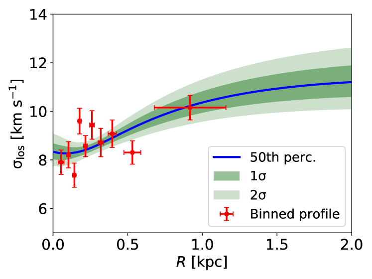
Figure 6: Line-of-sight velocity dispersion profile of Sculptor (dots) compared with that of our dynamical model (curve and bands). In the model we show the posterior distribution for $\sigma_{\text{los}}(R)$ obtained using the likelihood in Eq. 8 and assuming $D=86$ kpc as Sculptor distance (FH18 case, see Sec. 3.2). The line shows the median $\sigma_{\text{los}}(R)$, while dark and light green bands indicate, respectively, the $68\%$ ($1\sigma$) and $95\%$ ($2\sigma$) confidence intervals. The red points are the same as in Fig. 3, assuming $D=86$ kpc. We stress that the model does not fit the binned $\sigma_{\text{los}}$ profile but is determined using individually the line-of-sight velocities of Sculptor’s members.

The posterior distributions of the predicted velocity dispersion profile is shown in Fig. 6 for the FH18 case (see Sec. 3.2) compared with the observed velocity dispersion profile (Sec. 2.3.3). The results are similar also considering the Sculptor distance assumed in the EH18 orbit. The posterior distributions of $\,{r}_{\rm c}$ and $M_{\text{200}}$ indicate that these two parameters are quite correlated so that we can obtain similar results with a lower (higher) virial mass and a smaller (larger) core radius. However, in all the analysed cases the core radius is not compatible with 0, rather it is of the same order of the (projected) stellar half-light radius and it is about $8\%$ of the NFW scale length $r_{\text{s}}$.

The estimated core lengths are compatible with the theoretical predictions of transformation from primordial cuspy to cored DM density profiles due to effect of baryons (e.g. Nipoti & Binney 2015; Bermejo-Climent et al. 2018). The presence of a core in the DM halo model is needed to reproduce the velocity dispersion profile in the inner part of Sculptor (Fig. 6), at least under the assumption of isotropic stellar velocity distribution. In the case of cuspy DM profiles (like a pure NFW model), the galaxies result more resilient to the influence of the tidal fields (Peñarrubia et al., 2008, 2010; Frings et al., 2017). In this context, the presence of extended cores in our model DM halo is compatible with the conservative strategy to set up our simulation in the most favourable conditions to maximise the effect of tides. For this reason, we did not run simulations with “cuspy” DM halos.

In the case of FH18 (assumed distance $D=86.0$ kpc) we obtained $V_{\text{sys}}=111.4\pm 0.2\,{\rm km\,s}^{-1}$, $r_{\text{c}}=0.14\pm 0.05$ kpc and $\log\left(\,{M}_{200}/\,{\rm M}_{\odot}\right)=9.39\pm 0.10$ ($c=14.89$), while for EH18 ($D=82.3$ kpc) we obtained $V_{\text{sys}}=111.4\pm 0.2\,{\rm km\,s}^{-1}$, $r_{\text{c}}=0.15\pm 0.04$ kpc and $\log\left(\,{M}_{200}/\,{\rm M}_{\odot}\right)=9.41\pm 0.09$ ($c=14.83$). The systematic differences in the DM halo parameters are mostly due do the fact that, assuming different distances for Sculptor, the physical distribution of Sculptor’s members as well the physical scales (e.g. $\,{r}_{\rm c}$ and $b_{*}$) are stretched or shrunk (EH18) with respect to the fiducial case (FH18). The DM dynamical model adapts to these changes reducing (or increasing) the core length and increasing (or reducing) the virial mass. However, we verified that the mass within $r\approx 1\,{\rm kpc}$ (a radius containing most of Sculptor’s members) is essentially independent of the distance ($M_{\text{DM}}\sim 10^{8}\,{\rm M}_{\odot}$, in agreement with the estimate by Zhu et al. 2016). Recently, Errani et al. (2018) estimated $M_{\text{DM}}=3.16^{+0.82}_{-0.65}\times 10^{7}\,{\rm M}_{\odot}$ at radius $r=1.8R_{\text{h}}\approx 0.5\ \,{\rm kpc}$ using a method that minimises the uncertainties due to the assumptions on the DM halo parameters. This value is largely consistent with our mass estimate at the same radius: $M_{\text{DM}}=3.35\pm 0.12\times 10^{7}\,{\rm M}_{\odot}$ for FH18 and $M_{\text{DM}}=3.32\pm 0.12\times 10^{7}\,{\rm M}_{\odot}$ for EH18. We also estimated the slope of the mass profile as $\Gamma(r)={\rm d}\ln M_{\text{tot}}(r)/{\rm d}\ln r$, finding, at the half-light radius $r=R_{\text{h}}$, $\Gamma=2.07\pm 0.10$ for FH18 and $\Gamma=2.10\pm 0.10$ for EH18. Exploiting the presence of two distinct chemodynamical stellar populations in Sculptor (see Sec. 2 and Sec. 7) Walker & Peñarrubia (2011) used a non parametric method, based on the only assumption $M(\approx R_{\text{h}})\propto R_{\text{h}}\sigma^{2}_{\text{los}}$ (see also Errani et al. 2018), to measure $\Gamma=2.95^{+0.51}_{-0.39}$ at Sculptor’s half-light radius. Investigating possible systematic effects behind this discrepancy, we found that the main cause is a slight difference of the “average” measured velocity dispersion. In fact, we estimated the los velocity dispersion of the two components modifying the likelihood in Eq. 8 so that it includes two Gaussian components with (constant) velocity dispersion ($\sigma_{1}$, $\sigma_{2}$) and the relative component fractions are set using the best-fit radial profiles reported in Walker & Peñarrubia (2011). We found $\sigma_{1}=7.01\pm 0.4\ \,{\rm km\,s}^{-1}$ and $\sigma_{2}=10.35\pm 0.4\ \,{\rm km\,s}^{-1}$, while Walker & Peñarrubia (2011) measured $\sigma_{1}=6.4\pm 0.4\ \,{\rm km\,s}^{-1}$ and $\sigma_{2}=11.6\pm 0.6\ \,{\rm km\,s}^{-1}$. These differences could be caused by the methods used to take into account the Milky Way interlopers and/or of the outliers (see also Strigari et al., 2017). A detailed study of the internal dynamics and mass content of Sculptor, which is not the focus of this paper, could be improved through a complete analysis of the distribution of individual stellar velocities (see Pascale et al., 2018).

In order to analyse the effect of the the baryonic mass-to-light ratio on the results of the dynamical fitting, we repeated the fit (for the FH18 case) adding the baryonic mass-to-light ratio in the V-band, $\Upsilon_{*}$, as an additional parameter assuming the uniform prior $P(\Upsilon_{*})=\mathcal{U}(0.01,100)$. The final posterior distribution for $\Upsilon_{*}$ is quite broad and asymmetric with a peak at $\Upsilon_{*}\approx 7$, a rapid decrease down to extreme values ($\Upsilon_{*}\approx 16$) and a more “gentle” decrease toward lower values. In conclusion, the addition of $\Upsilon_{*}$ as free parameter increases the uncertainties on the values of the DM halo parameters, but it does not improve significantly the quality of the fit (similar value of the best likelihood). In particular, if we limit the analysis to realistic $\Upsilon_{*}$ values (e.g. from few tenth to 4) the final maximum likelihoods are very similar. Hence, we decided to fix the mass-to-light ratio to $\Upsilon_{*}=2$ in the following $N$-body simulations (with the only exception of the mass-follows-light models of Sec.  6.4).

5 $N$-body Simulations

In order to investigate the effects of the Milky Way tidal field on the structure and kinematics of Sculptor, we ran a set of $N$-body simulations putting Sculptor-like objects in observationally motivated orbits (Sec. 3.2) around the Milky Way (Sec. 3.1). Our work is analogous to the investigation of the effect of tides on Fornax by Battaglia et al. (2015). Following that work, we iteratively changed the initial conditions of the Sculptor-like objects to reproduce the observed position and the observed properties of Sculptor (Tab. 1) in the last snapshot of the simulations. Finally, considering the known “intrinsic” properties of the simulated objects, we investigated whether the observed kinematics of the stars is a robust tracer for the current dynamical state of Sculptor (in other words, whether Sculptor can be considered stationary) or the tides are introducing non-negligible biases.

5.1 $N$-body realisations of Sculptor

The initial conditions for each $N$-body realisation of Sculptor have been produced using the Python module OpOpGadget developed by G. Iorio. The radii of the star and DM particles are randomly drawn to reproduce the input densities $\rho_{*,\text{Nb}}(r)$ and $\rho_{\text{DM},\text{Nb}}(r)$, respectively. Then, we assign to each star the spherical angles $\phi$ (azimuthal angle) and $\theta$ (zenithal angle) picking randomly from the uniform distributions $P(\phi)=\mathcal{U}(0,2\pi)$ and $P(\cos\theta)=\mathcal{U}(-1,1)$. In this way, we sample uniformly the sphere at each radius obtaining a spherical distribution of matter. Finally, the Cartesian coordinates are obtained as $x=r\sin\theta\cos\phi$, $y=r\sin\theta\sin\phi$ and $z=r\cos\theta$. In the next step, the velocity components of each star are assigned through an acceptance-rejection technique assuming isotropy and using the two-component ergodic distribution functions obtained with Eddington’s inversion (Binney & Tremaine, 2008). Once the positions and velocities have been assigned to each particle, the position ($r_{\text{COM}}$) and the velocity ($V_{\text{COM}}$) of the centre of mass (COM) are estimated and the phase-space coordinates of the particles are translated to correct for any “residual” displacement from $r_{\text{COM}}=0$ and $V_{\text{COM}}=0$. The method produces spherical and isotropic $N$-body realisations of systems in equilibrium, as we verified by running simulations with the same initial conditions of those presented in this work, but in isolation, i.e. without the MW external potential.

We produced Sculptor-like objects using the stellar density law

$$\rho_{*,\text{Nb}}(r;M_{*},b_{*})=\rho_{*}(r;M_{*},b_{*})\exp\left[-\left(\frac{r}{r_{\text{t}}}\right)^{2}\right],$$ (9)

where $\rho_{*}$ is the Plummer profile in Eq. 2, $M_{*}$ indicates the mass enclosed within the projected radius $R_{*}=1.5^{\circ}$ and $b_{*}$ is the Plummer core radius (see Sec. 4.1.1). Similarly, for the DM halo we used

$$\rho_{\text{DM},\text{Nb}}(r;\,{M}_{200},\,{r}_{\rm c})=\rho_{\text{DM}}(r;\,{M}_{200},\,{r}_{\rm c})\exp\left[-\left(\frac{r}{r_{\text{t}}}\right)^{2}\right],$$ (10)

where $\rho_{\text{DM}}$ is the cored NFW profile in Eq. 5 and the parameters $\,{M}_{200}$ and $\,{r}_{\rm c}$ indicate the virial mass and the halo core radius (see Sec. 4.1.2), respectively. The truncation radius is needed because both the Plummer and the NFW profile have a non-negliglible probability to have particles up to infinity. In particular the NFW mass diverges when $r\rightarrow\infty$. Moreover, from a physical point of view, the DM halo of Sculptor is expected to be truncated due to the presence of the Milky Way. We set $r_{\text{t}}=8.5\ \,{\rm kpc}$ for FH18 and $r_{\text{t}}=6.0\ \,{\rm kpc}$ for EH18, which, at the starting positions of the simulations, are of the order of (but slightly larger than) the Jacobi radius in the restricted three-body problem (the primary bodies are the MW and Sculptor, while the third body is a Sculptor’s star, see Binney & Tremaine 2008). The specific choice of the values of $r_{\text{t}}$ is not expected to be important for the final results of this work, because most of the DM halo particles close or beyond the truncation radius are stripped during the pericentric passages. Moreover, since the assumed truncation radii are much larger than the other involved physical scales ($b_{*}$, $\,{r}_{\rm c}$), we are confident that the presence of a density truncation does not have any effect on the results of the dynamical fit in Sec. 4.

For each $N$-body realisation we used $N_{*}=5\times 10^{4}$ stellar particles and $N_{\text{DM}}=4\times 10^{6}$ DM particles. Since the total masses of the stellar and DM components change in the different analysed cases (FH18, EH18) and in different stages of the iterative process, the mass ratio between DM and stellar particles changes accordingly. It ranges between $\approx 2.5$ for the first run of EH18 and $\approx 8$ for the last run of EH18 (see Col. 8 in Tab. 4). We re-run the simulations of the last iterative steps of FH18 and EH18 halving the number of star particles ($N_{\text{*}}=2.5\times 10^{4}$) to halve the DM to stellar particle mass ratio. The properties of the last snapshots of these additional simulations are compatible with the results presented in the following sections. Therefore we conclude that the results of this work (see Sec. 6) are not influenced by the adopted particle mass ratios.

5.2 Set up of the simulations

5.2.1 $N$-body code

The simulations have been performed using the collisionless code FVFPS (Londrillo et al., 2003; Nipoti et al., 2003) with the addition of the J95 Milky Way model (see Sec. 3.1) as external potential (Battaglia et al., 2015). We adopted $\theta_{\text{min}}=0.5$ as the minimum value of the opening parameter and we fixed the softening parameter to $\epsilon=10\ \text{pc}$. We decided to use a constant time step, $\Delta t=0.03t_{\text{dyn}}$, where

$$t_{\text{dyn}}=\sqrt{\frac{1}{G\bar{\rho}_{\text{h}}}}$$ (11)

is the initial dynamical time (Binney & Tremaine, 2008) of the Sculptor-like system and $\bar{\rho}_{\text{h}}$ is the average 3D density estimated considering the total matter (stars and DM) content within the stellar half-mass radius $r_{\text{h}}$. The dynamical time depends on the initial conditions of the $N$-body realisations, varying between $\approx 3\times 10^{5}\ \text{yr}$ and $\approx 5\times 10^{5}\ \text{yr}$ (see Col. 9 in Tab. 4).

We do not include the gas in our simulations. However, we note that the star formation in Sculptor was already almost turned-off 8 Gyr ago (roughly the starting time of our simulations), hence it is likely that, in the analysed time window, the gas was already absent or negligible with respect to the stellar and DM components.

5.2.2 Initial phase-space coordinates

We ran a series of simulations considering the two different orbital cases discussed in Sec. 3.2 and summarised in Tab. 3. In each of the simulations, we set the initial phase-space coordinates of the $N$-body realisations at the first apocentre occurred within a lookback time of 8 Gyr. The FH18 represents the fiducial orbit obtained considering the nominal proper motion reported in H18 and the nominal Milky Way parameters (see Sec. 3.1). The Sculptor-like object is placed at $(x,y,z)=(-12.43,\ 98.05,\ -36.70)\ \text{kpc}$ with initial velocity $(V_{x},V_{y},V_{z})=(-11.67,\ 44.19,\ 130.03)\ \,{\rm km\,s}^{-1}$. The EH18 represents one of the most extreme (at $3$-$\sigma$ level) eccentric orbit compatible with the H18 proper motion measurements and with the errors on the Milky Way parameters. The starting position is at $(x,y,z)=(-8.21,\ 26.56,\ 90.33)\ \text{kpc}$ and the initial velocity vector is $(V_{x},V_{y},V_{z})=(13.34,\ -109.23,\ 33.03)\,{\rm km\,s}^{-1}$.

5.2.3 Dynamical friction

In the orbital investigation described in Sec. 3, we have not considered dynamical friction (Binney & Tremaine, 2008), which could affect the orbits of massive satellites, like dwarfs, reducing their pericentre, and thus leading to stronger tidal effects. We can have an estimate of the dynamical friction time scale at a given Galactocentric radius, $r_{\text{g}}$, using equation (8.13) in Binney & Tremaine (2008):

$$t_{\text{f}}(r_{\text{g}})=\frac{1.17}{\ln\Lambda}\frac{M_{\text{MW}}(<r_{\text{g}})}{M_{\text{Scl}}}t_{\text{cross}}(r_{\text{g}}),$$ (12)

where $M_{\text{MW}}(<r_{\text{g}})$ is the Milky Way mass within a sphere of radius $r_{\text{g}}$ and $M_{\text{Scl}}$ is the total mass of Sculptor estimated at the truncation radius (see Sec. 4.3 and Sec. 5.1). The crossing time, $t_{\text{cross}}$, is defined as $r_{\text{g}}/v_{\text{c}}$, where $v_{\text{c}}=\sqrt{GM_{\text{MW}}(<r_{\text{g}})/r_{\text{g}}}$ is the circular speed at $r_{\text{g}}$. The Coulomb logarithm $\ln\Lambda=\ln b_{\text{max}}/b_{\text{90}}$ is estimated assuming maximum impact parameter $b_{\text{max}}=r_{\text{g}}$ and deflection radius $b_{\text{90}}$ equal to the half-mass (stars+DM) radius of Sculptor, $r_{\text{h,tot}}$. At the apocentres of the considered orbits ($r_{\text{g}}\approx 100\ \text{kpc}$, see Tab. 3.1) $M_{\text{MW}}\approx 9\times 10^{11}\ \,{\rm M}_{\odot}$, $r_{\text{t}}\approx 6-12\ \text{kpc}$, $M_{\text{Scl}}\approx 1-9\times 10^{9}\,{\rm M}_{\odot}$ and $r_{\text{h,tot}}\approx 3-5\ \text{kpc}$; while, at the pericentres ($r_{\text{g}}\approx 40\ \text{kpc}$, see Tab. 3.1) $M_{\text{MW}}\approx 4\times 10^{11}\ \,{\rm M}_{\odot}$, $r_{\text{t}}\approx 2-4\ \text{kpc}$, $M_{\text{Scl}}\approx 0.3-2.0\times 10^{9}\ \,{\rm M}_{\odot}$ and $r_{\text{h,tot}}\approx 1-3\ \text{kpc}$. The value of $t_{\text{f}}$ depends on the details of the considered family of simulations (FH18 or EH18), but we found that, considering both the apocentre and the pericentre, the dynamical friction time scale is always $t_{\text{f}}>13\ \text{Gyr}$. In conclusion, since the dynamical friction does not cause an appreciable difference in shaping the orbit of Sculptor, for simplicity we did not consider it in our simulations, in which the MW is represented by a fixed gravitational potential.

5.3 Iterative method

Following Battaglia et al. (2015) we have set up an iterative procedure in which we tune the initial parameters of the $N$-body realisations (Sec. 5.1) to reproduce in the last snapshot of the simulations the observed Sculptor properties, namely the position on the sky, the systemic velocity, the proper motions, the projected surface density, the los velocity dispersion profile and stellar mass (see Tab. 1). The steps of the iterative procedure are as follows.

1. For the first simulation, we make the $N$-body realisation assuming the stellar mass ($M_{*}=4.6\times 10^{6}\ \,{\rm M}_{\odot}$ within $R_{*}=1.5^{\circ}$, see Sec. 4.1.1) and the Plummer core length ($b_{*}=10.15\arcmin$) estimated from the observations. Concerning the DM halo parameters $\,{r}_{\rm c}$ and $\,{M}_{200}$, we use the values estimated from the dynamical models fitting in Sec. 4.3. The initial position and the initial velocity are set as described in Sec. 5.2.2. Accordingly, the initial integration time, $t_{\text{sim}}$, of each simulation is set to reproduce the current Sculptor position and velocities in the last snapshot ($t_{\text{sim}}=6.9$ Gyr for FH18 and $t_{\text{sim}}=7.2$ Gyr for EH18, see Sec. 3.2). However, they can change at different stages of the iterative process; see (iii) for further details.

2. At the end of each simulation, we use the tools developed in OpOpGadget to “simulate” an observation projecting the stellar particles on the plane of the sky (see Appendix A). We assume the centre of the Sculptor realisation as the position of the centre of the system (COS) of the stellar particle distribution (roughly, the peak of the stellar density) estimated with the iterative technique of Power et al. (2003). We define the COS velocity, as the mean velocity of the particle selected in the last iteration of the Power et al. (2003) technique. Then, we measure the stellar mass $M_{*,\text{sim}}$ within the projected radius $R_{*}=1.5^{\circ}$, the projected half-light radius $R_{\text{h,sim}}$ and two values of the los velocity dispersion, $\sigma_{\text{los,sim}}(<R_{\text{h,sim}})$ and $\sigma_{\text{los,sim}}(<R_{*})$, estimated considering all the stars within $R_{\text{h,sim}}$ and $R_{*}$, respectively.

3. Each one of the observed parameters is sensitive mostly to a particular dynamical parameter, thus we update our dynamical model using

   $$b_{*,\text{i+1}}=b_{*,\text{i}}\frac{R_{\text{h}}}{R_{\text{h,sim}}},\\ M_{*,\text{i+1}}=M_{*,\text{i}}\frac{M_{*}}{M_{\text{*,sim}}},\\ r_{\text{c},\text{i+1}}=r_{\text{c},\text{i}}\frac{\sigma_{\text{los,sim}}(<R_{\text{h,sim}})}{\sigma_{\text{los}}(<R_{\text{h}})},\\ M_{\text{vir},\text{i+1}}=M_{\text{vir},\text{i}}\frac{\sigma_{\text{los}}(<R_{*})}{\sigma_{\text{los,sim}}(<R_{*})},\\$$ (13)

   where with the index $i$ we refer to the values used to make the currently analysed $N$-body realisation. Due to the gravitational effect of the DM particles lost in the tidal tails, it is not guaranteed that the COS of the stellar distribution matches perfectly the current position of Sculptor in the last snapshot. In fact, at the end of the simulations the COS position is still close to the predicted orbital track (Sec. 3), but ahead or behind with respect to the expected position. In other terms, this effect introduces a time offset ($\Delta t\approx 10-300$ Myr) between the integration time predicted in the simple point-like orbit integration (Sec. 3) and the integration time of the simulation, $t_{\text{sim}}$, needed to bring the simulated object in the observed Sculptor position. We take into account this effect updating the integration time of the simulation as

   $$t_{\text{sim,i+1}}=t_{\text{sim,i}}-\Delta t.$$ (14)

The steps (ii) and (iii) are repeated until the sum of the relative differences between the observed quantities and those “observed” in the last snapshot of the simulation (see Eqs.  LABEL:eq:pcorr) are no longer improved by the iterative procedure. The simple time correction implemented with Eq. 14 is able to tune the simulation integration time so that in the last snapshot of all our final (last iteration) simulations the COS position and the COS velocity nicely match (relative errors within $5\%$) the observed position, the systemic velocity and the proper motion of Sculptor (see Sec. 6.1).

6 Results

	$M_{*}$ [$10^{6}\ \text{M}_{\odot}$] (1)	$b_{*}$ [kpc] (2)	$M_{*,\text{tot}}$ [$10^{6}\ \text{M}_{\odot}$] (3)	$M_{\text{200}}$ [$10^{9}\ \text{M}_{\odot}$] (4)	$r_{\text{c}}$ [kpc] (5)	$c$ (6)	$M_{\text{DM},\text{tot}}$ [$10^{9}\ \text{M}_{\odot}$] (7)	$M_{\text{tot}}(<1\ \text{kpc})$ [$10^{8}\ \text{M}_{\odot}$] (8)	$f_{\text{p}}$ (9)	$t_{\text{dyn}}$ [Myr] (10)	$t_{\text{sim}}$ [Gyr] (11)	$f_{*}$ $(<1\ \text{kpc},<2\ \text{kpc})$ (12)	$f_{\text{DM}}$ $(<1\ \text{kpc},<2\ \text{kpc})$ (13)
[HTML]C0C0C0 FH180	4.60	0.28	4.68	2.45	0.14	14.89	1.01	1.04	2.69	53.8	6.85	(96%, 98%)	(65%, 55%)
FH1814	4.62	0.26	4.69	6.31	0.13	13.80	1.95	1.49	5.20	44.69	6.79	(97%, 99%)	(69%, 60%)
[HTML]C0C0C0 EH180	4.60	0.27	4.68	2.57	0.15	14.83	0.84	1.05	2.23	52.41	7.19	(89%, 91%)	(37%, 23%)
EH1817	4.66	0.22	4.71	22.39	0.12	12.38	2.94	2.23	7.81	35.76	7.07	(95%, 98%)	(45%, 35%)

Table 4: Summary of simulation properties. For each analysed orbit (FH18 and EH18, see Tab. 3), we report data for the first and the last simulations in the iterative cycle (Sec.  5.3) as indicated by the subscript. (1)(2) stellar mass within $R_{*}=1.5^{\circ}$ and core radius of the initial 3D stellar density profile (Eq. 2 and Eq. 9); (3) total stellar mass ($5\times 10^{4}$ stellar particles); (4)(5)(6) viral mass, core radius and concentration parameter of the initial 3D DM density profile (see Sec. 4.1.2, Eq. 5 and Eq. 10); (7) DM total mass ($4\times 10^{6}$ DM particles); (8) total mass enclosed within $r=1$ kpc at $t=0$; (9) DM-to-stellar particle mass ratio; (10) initial dynamical time (it is used to set the simulation time step, see Sec. 5.2.1); (11) simulation integration time; (12) fraction of the initial stellar mass retained within (1, 2) kpc in the last snapshot ($t=t_{\text{sim}}$); (13) same as Col. (12), but for the DM mass.

In this Section, we present the results of the the families of simulations FH18 and EH18 whose properties and initial set-ups are described in Sec. 3.2 and Sec. 5. A subscript in the simulation name indicates what stage of the iterative cycle (Sec. 5.3) we are referring to. The index 0 indicates the initial runs performed using the parameters obtained from the observations (see Tab. 3 and Sec. 4.3; e.g. FH18₀ indicates the first simulations considering the FH18 orbit).

6.1 Results of the iterative process

The convergence of the iterative processes (Sec. 5.3) has been reached after 14 iterative steps considering the fiducial orbit FH18 and after 17 steps for the more eccentric EH18 orbit. Fig. 7 shows that, overall, the “observed” properties of the last snapshots of the simulations FH18₁₄ and EH18₁₇ nicely agree with the observed properties of Sculptor. The final positions of the simulated objects are slightly off-set with respect to the current Sculptor position, especially in the EH18₁₇ simulation ($\approx 30\arcmin$), due to the mismatch between the simulation orbit and the single-particle orbit (Sec. 3.2), as discussed in Sec. 5.3. However, the distribution of the stellar particles and the kinematic properties (proper motions, velocity dispersion profile) show an almost perfect agreement.

Within the radial extent of the Sculptor dataset ($R_{*}=1.5^{\circ}$) the iso-density contours of the simulated objects remain smooth and there are no signs of tails. Even beyond this radius, neither the distribution of stars nor the stellar kinematics shows evident sign of tidal disturbance. This is the case for both the fiducial orbit FH18 and the more eccentric orbit EH18. Beyond $R\approx 2^{\circ}$ the $\sigma_{\text{los}}$ profiles are inflated due to the combination of few stars escaping from the system and the small number of tracers that increases the amplitude of statistical oscillations (see the simulation videos, links at the end of Sec. 6.2).

Most of the stellar particles remains bound during the orbit integrations: at the end of the simulations only few percent of the stellar mass is lost considering a radius of 2 kpc as a boundary (see Tab. 4). This can be easily understood since the minimum truncation radius (estimated as the Jacobi radius, see Sec. 5.1) at the pericentre of the orbits ($r_{\text{t}}\approx 3\ \,{\rm kpc}$) is about twice the radius containing the bulk ($\approx 99\%$, see Fig. 9) of the stellar mass. We conclude that, given the current position of Sculptor and the most recent estimate of its proper motions, it is very likely that it has not developed any strong stellar tails due to the interaction with the Milky Way tidal field. As a consequence, the spectroscopic dataset of Sculptor, as the one used in this work (Sec. 2.3), should not be contaminated significantly by tidally stripped stars.

At the end of iterative procedure the initial DM halo has $r_{\text{c}}=0.13$ kpc and $M_{\text{200}}=6.31\times 10^{9}\ \,{\rm M}_{\odot}$ (total mass of $1.95\times 10^{9}\ \,{\rm M}_{\odot}$ considering the truncation) for FH18₁₄ and $r_{\text{c}}=0.12$ kpc and $M_{\text{200}}=2.24\times 10^{10}\ \,{\rm M}_{\odot}$ (total mass of $2.94\times 10^{9}\ \,{\rm M}_{\odot}$ considering the truncation) for EH18₁₇ (see Tab. 4).

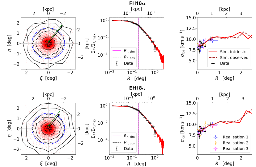
Figure 7: “Observed” properties (see Appendix A) of the last snapshot of the $\text{FH18}_{\text{14}}$ (upper panels) and $\text{EH18}_{\text{17}}$ (lower panels) simulations. Left-hand panels: distribution of the stellar particles in the sky-projected equatorial $\xi-\eta$ plane (see Fig. 2); the dashed circle with radius $R_{*}=1.5^{\circ}$ is centred on the projected COS (see Sec. 5.3); the green square indicates the observed position of Sculptor with respect to the COS; the arrows indicate the direction of Sculptor’s proper motion (green-thin line) and of the proper motion of the COS (black-thick line). Both proper motions have been corrected for the solar motions. The length of the arrows is proportional to the proper motion magnitude. The black iso-density contours indicate regions where the surface density is the (0.005, 0.01, 0.05, 0.1, 1, 10, 25, 50, 90) percent of the maximum value. Middle panels: “observed” surface density profile of the stellar particles (red line) compared with the (rescaled) Sculptor data (see Sec. 2.1); the vertical lines indicate the half-light radius measured for Sculptor (black-dashed) and estimated from the stellar particles (magenta), the two radii differ by less than 0.01 %. Right-hand panels: “observed” (brown-dashed line) and intrinsic (i.e. corrected for the Sun motion, red line) $\sigma_{\text{los}}$ profile of the stellar particles compared with the binned $\sigma_{\text{los}}$ profile of Sculptor (black points); the blue, yellow and magenta points represent binned profiles estimated with sub-samples of stellar particles (see Sec. 6.3) using the technique described in Sec. 2.3.3

6.2 The evolution of the stellar and DM components

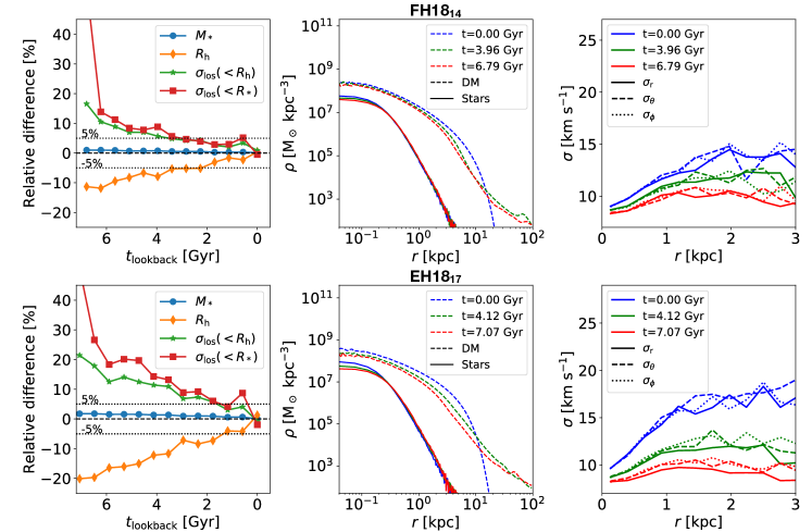
Figure 8: Time evolution of the properties of the FH18₁₄ (upper panels) and EH18₁₇ (lower panels) simulations. Left-hand panels: relative difference between the “observed” properties (see Appendix 1) of the stellar particles in the simulation and the related properties observed in Sculptor (see Tab. 1): stellar mass within $R_{*}=2.25\ \text{kpc}$ for FH18₁₄ and $R_{*}=2.15\ \text{kpc}$ for EH18₁₇ (blue circles), half-light radius $R_{\text{h}}$ (orange diamonds), los velocity dispersion profile within $R_{\text{h}}$ (green stars) and within $R_{*}$ (red squares); the value of $R_{*}$ is different for FH18₁₄ and EH18₁₇ because it is based on the definition of $R_{*}=1.5^{\circ}$ and the current assumed distance of Sculptor (see Sec. 2.3.2 and Tab. 3); see caption of Fig. 4 for the definition of $t_{\text{lookback}}$. Middle panels: 3D density profiles of the DM (dashed lines) and stellar (solid lines) particles at different times (initial conditions, blue lines; last snapshot, red lines; intermediate time, green lines). Right-hand panels: radial profile of the velocity dispersion components in spherical coordinates centred on the COS defined in Sec. 5.3 ($\sigma_{\text{r}}$, solid lines; $\sigma_{\theta}$ dashed lines; $\sigma_{\phi}$ dotted lines) at different times (initial conditions, blue lines; last snapshot, red lines; intermediate time, green lines).

During the orbital evolution, the extended DM halo is influenced by tides quite instantaneously developing significant trailing and leading tails. Fig. 8 shows that the density profile of the DM in FH18₁₄ evolves mostly in the outer part due to tidal stripping, while the strong tidal shocks experienced by the satellite in EH18₁₇ (due to the smaller pericentric radius ) cause also a significant depletion of DM mass in the innermost part. At the end of the simulations the fraction of initial DM mass retained within 2 kpc is 60% in FH18₁₄ and only $35\%$ in EH18₁₇ (see Tab. 4). Most of the evolution of the DM halo happens at the pericentric passages where the halo is heated by tidal shocks and it expands increasing the core radius, meanwhile in outer parts, it loses mass due to tidal stripping. Therefore, in order to reproduce the current properties of Sculptor, we had to start our simulations with smaller DM core radius and a larger DM total mass (about 2 and 3 times larger for FH18 and EH18, respectively, see Tab. 4).

Figs.  8 show cleary that, in both the FH18 and the EH18 simulations, the stellar component is not strongly affected by the MW tidal field. In particular, the left-hand panels of Fig. 8 show that the mass evolution within $R\approx 2\ \text{kpc}$ is almost negligible: only few stellar particles are stripped during the evolution ($\approx 1\%$ for FH18₁₄ and $\approx 2\%$ for EH18₁₇), so no stellar tidal signatures are visible in the last snapshots of the simulations (see Sec. 6.1). However, the evolution of the DM halo and the subsequent variation of the gravitational potential force the stellar component to find a new equilibrium modifying both its structure and its kinematics (Peñarrubia et al., 2008, 2009b; Battaglia et al., 2015). The stellar distribution tends to expand: in particular, the half-light radius increases by about 10% in FH18₁₄ and about 20% in EH18₁₇ as shown in the left-hand panel of Fig. 8. The DM loss and the evolution of the DM density distribution causes a decrease of all the velocity dispersion components (right-hand panels of Fig. 8). As a consequence, the los velocity dispersion decreases both in the inner parts (within the half-light radius) and in the outer parts (within $R\approx 2\ \text{kpc}$) by about 15-20 % in FH18₁₄ and about 25-30 % in EH18₁₇ considering the last $\approx 6$ Gyr of orbital evolution.

We analysed also the evolution of the shape and of the anisotropy of the stellar component. During the orbital evolution the stellar axial ratios remain close to the initial value of 1, more precisely they oscillate between 0.93 and 1 both in FH18₁₄ and EH18₁₇. Therefore, the flattening observed in Sculptor is likely an intrinsic property of Sculptor, rather than induced by tides (but see Sanders et al. 2018 for further details on the shape evolution of satellites in the MW tidal field). Concerning the stellar velocity anisotropy, the right-hand panels of Fig. 8 show that the values of the three spherical velocity dispersion components in the Sculptor frame of reference, $\sigma_{\text{r}}$, $\sigma_{\theta}$ and $\sigma_{\phi}$, remain close to each other for FH18₁₄ (i.e. the system remains isotropic) both in the intermediate and in the last phase of the orbital evolution. Concerning EH18₁₇, in the last phases of the orbital evolution, the velocity dispersion along the radial direction tends to be slightly lower with respect to the tangential components resulting in a slightly tangentially anisotropic system. This is expected since the few stars that are lost in tails are preferentially the ones in radial orbits (Takahashi & Lee, 2000; Baumgardt & Makino, 2003). Both in FH18 and EH18 The differences between the three components become larger at large radii ($r>2\ \text{kpc}$), but this is mainly due to the increase of the Poisson noise: the same trend is apparent at $t=0\ \,{\rm Gyr}$, when the system is isotropic by construction (see Sec. 5.1).

Overall the main properties of the stellar component of the simulated Sculptor-like objects have changed very little (<10%) in the last 3-4 Gyr (see left-hand panel of Fig. 8). Therefore, we conclude that Sculptor can be reasonably well modelled as an isolated system in equilibrium.

Videos of the evolution of the simulations FH18₁₄ and EH18₁₇ can be found online at https://doi.org/10.5446/40807 and https://doi.org/10.5446/40808, respectively.

6.3 Dynamical fit to the final snapshot

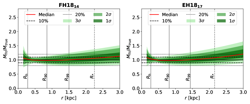
Figure 9: Ratio between the mass profile estimated from the dynamical fit and the true mass distribution in the last snapshot of the simulations FH18₁₄ (left-hand panel) and EH18₁₇ (right-hand panel). For each simulation we applied the dynamical fit procedure described in Sec. 4.2 to 300 sub-samples of stellar particles selected to match the properties of our Sculptor dataset (Sec. 2.3.2, see text for further details). The red curve (median) and the green bands ($1\sigma$, $2\sigma$, $3\sigma$ levels) show the posterior distribution of the ratio between the mass profiles estimated using the 300 best-fit DM halo parameters and the true total mass distribution. The dashed and dotted horizontal lines highlight the regions where the mass differences are lower than 10% and 20%, respectively. The grey vertical lines indicate the median (over the 300 sub-samples) of the projected radii containing the $50\%$ ($R_{\text{h}}$), the $90\%$ ($R_{\text{90}}$) and the $99\%$ ($R_{\text{99}}$) of the stellar particles in the sub-samples. The grey vertical-dashed line indicate the projected $R_{*}=1.5^{\circ}$ that represents roughly the radial extent of our dataset (see Sec. 4.1.1).

As an additional test for the dynamical state of Sculptor, we repeated the dynamical modelling applied to the data and described in Sec. 4.2 to the stellar particles in the last snapshot of the FH18₁₄ and EH18₁₇ simulations. In order to take into account the uncertainty due to the observational errors and data sampling, we did not use the complete sample of stellar particles, but rather we obtained 300 sub-samples as follows. (i) We bin the stellar particles using the same bin edges applied to the data to estimate the velocity dispersion profile (see Sec. 2.3.3); (ii) for each sub-sample we randomly select a number of stars in each of the ten bins to match the number of stars in the observational data (192 particles in the last bin and 150 in the others); (iii) For each star we add Gaussian noise to the particles $V_{\text{los}}$ picking randomly from the $V_{\text{los}}$ errors distribution of the observational data (mean $\approx 2.3\ \,{\rm km\,s}^{-1}$ and standard deviation $\approx 2\ \,{\rm km\,s}^{-1}$).

At the end of this procedure, we obtain 300 sub-samples with stellar particles distributed along the projected radius roughly as the stars in our observed sample (see Sec. 2.3.2) and with errors that match the error distribution of the data. The velocity dispersion profiles estimated from three of these sub-samples can be seen in right-hand panels of Fig. 7. We notice that the incomplete sampling causes fluctuations on the binned velocity dispersion profile so that at given bin different realisations can differ more than 1$\sigma$, where $\sigma$ is the error estimated as for the data (see Sec. 2.3). These large fluctuations are often seen in binned profiles of dwarf galaxies (e.g.  Walker et al., 2009b), therefore one should be careful to interpret them as real kinematic features. Finally, we applied exactly the same fitting procedure described in Sec. 4.2 to each sub-sample. Given the best-fit halo parameters ($r_{\text{c}}$ and $M_{\text{vir}}$), using Eq. 2 and Eq. 5 we computed 300 (total) radial profiles of the total mass $M_{\text{fit}}$. Fig. 9 shows the comparison between $M_{\text{fit}}$ and $M_{\text{true}}$ estimated using the radial distribution of the stellar and DM particles in the last snapshot of the FH18₁₄ and EH18₁₇ simulations. Overall the two values show a good agreement. In particular, in the regions well sampled by the data (within $R_{90}\approx 0.57^{\circ}\approx 0.8\ \text{kpc}$) the median of the mass ratio is everywhere $\approx 1$ and the errors due to the incomplete sampling are within the $20\%$ at $3\sigma$ level. Fig. 9 shows that beyond $R_{99}\approx 1^{\circ}\approx 1.5\ \text{kpc}$, where there are few tracers, the mass content tend to be only slightly overestimated (by $10-20\%$). This test confirms the previous results (see Sec. 6.2) indicating that tidal effects are not significant at the present-day position of Sculptor and along orbits compatible with the most recent proper motion estimates (H18, F18) and implies that Sculptor can be reliably modelled assuming that it is isolated and stationary.

6.4 Mass-follows-light models

So far we have assumed a cosmologically motivated DM halo of the satellite, which is much more extended than the baryonic component. In this case, we demonstrated that the DM halo is able to “shield” the baryonic part of the satellite from the tidal field of the MW. It is possible that, in absence of an extended DM halo, the tidal force can be effective enough to produce a flat and high los velocity dispersion profile (Aaronson, 1983). This kind of model has been used by Muñoz et al. (2008) to obtain a good match to the observed properties of Carina dSph (but see Ural et al. 2015 for an alternative model including an extended DM halo). To explore this idea for Sculptor, we performed an additional suite of simulations assuming that the “mass follows light”. In these models the $N$-body realisation of the satellite is obtained as one-component isotropic system following the Plummer density profile in Eq. 9. We considered two cases, in one we assume a mass-to-light ratio $\Upsilon_{*}=2$ corresponding to a mass within $R_{*}=1.5^{\circ}$ of $M_{*}=4.6\times 10^{6}\,{\rm M}_{\odot}$, in the other we assume a mass-to-light ratio $\Upsilon_{*}=12$ corresponding to $M_{*}=2.76\times 10^{6}\,{\rm M}_{\odot}$. In the first case we are considering a pure baryonic representation of Sculptor, while in the second case the high $\Upsilon_{*}$ (not realistic for a pure baryonic component) is the value needed to reproduce the $\sigma_{\text{los}}\approx 8-9\ \,{\rm km\,s}^{-1}$ in the innermost part of system without an extended secondary component (see Sec. 4.3). In order to maximise the influence of tides, we put the two models in the eccentric EH18 orbit (Sec. 3) and we applied the same iterative approach used for the two-component models (Sec. 6.1) and described in Sec. 5.3. We found that it is not possible to obtain a perfect match considering together the total light (or baryonic mass) within $R_{*}=1.5^{\circ}$, the surface density profile and the los velocity dispersion profile. In particular, if we add more mass from the beginning, the system becomes more resilient to the tides so it is easy to match the observed surface density profile at the end of the simulations, but at the same time, we end with too much mass inside $R_{*}=1.5^{\circ}$. Tuning the initial mass to have the right amount of mass inside $R_{*}$, we could create a system in which the final surface density profile is distorted by a large amount of tidally stripped stars. For this reason, the iterative steps have been halted after three runs for both models.

The results of these simulations are shown in Fig. 10. In both cases, the tidal stripping is effective enough to produce tidal tails that are particularly significant in the case with $\Upsilon_{*}=2$ (left-hand panels in Fig. 10). In this model, the tidal tails starts to effectively “alter” the surface density profile around $R=0.6^{\circ}-0.7^{\circ}$ well inside the region covered by the photometric observations (Sec. 2.1). The mass loss is highly significant in the model with $\Upsilon_{*}=2$ ($\approx 50\%$) and more moderate in the model $\Upsilon_{*}=12$ ($\approx 10\%$). The innermost part is less affected by the tides, but the mass loss causes the half-light radius to shrink during the orbital evolution (about 20% for $\Upsilon_{*}=2$ and about 5% for $\Upsilon_{*}=12$). The velocity dispersion profile remains similar to the initial one in the innermost part ($R\lesssim 0.8^{\circ}$) showing just a slightly decreasing trend with time (<10%) in the case with $\Upsilon_{*}=2$. Therefore, in the last snapshots, the los velocity dispersion profiles are still significantly decreasing with radius for both models and significantly lower than the Sculptor $\sigma_{\text{los}}$ for the model with $\Upsilon_{*}=2$. Hence, neither model matches the los velocity dispersion profile of Sculptor (see right-hand panels in Fig. 10). We also notice that the fact that the velocity dispersion is not enhanced in the inner parts means that the tidal tails are not aligned along the los (Klimentowski et al., 2007). At large radii ($R\gtrsim 0.6-0.8^{\circ}$), where the sample starts to be contaminated by stripped stars, the los velocity dispersion profiles of the simulations reverse the radial trend and start to increase with radius. However, the $\sigma_{\text{los}}$ typical of Sculptor ($\sigma_{\text{los}}\approx 8-9\ \,{\rm km\,s}^{-1}$) are reached only in the very external regions ($R\approx 2.5^{\circ}$) of the model with $\Upsilon_{*}=12$, far beyond the regions covered by kinematic observations (right-hand panels in Fig. 10).

In conclusion, we found that, even in the absence of an extended halo component, the high-amplitude and flat observed velocity dispersion profile of Sculptor cannot be due to the effect of MW tides. Once again, this confirms that the Sculptor kinematic sample (Sec. 2.3.2) is practically free of contamination by tidally stripped stars.

A video of the evolution of the simulations with $\Upsilon_{*}=2$ can be found online at https://doi.org/10.5446/40809.

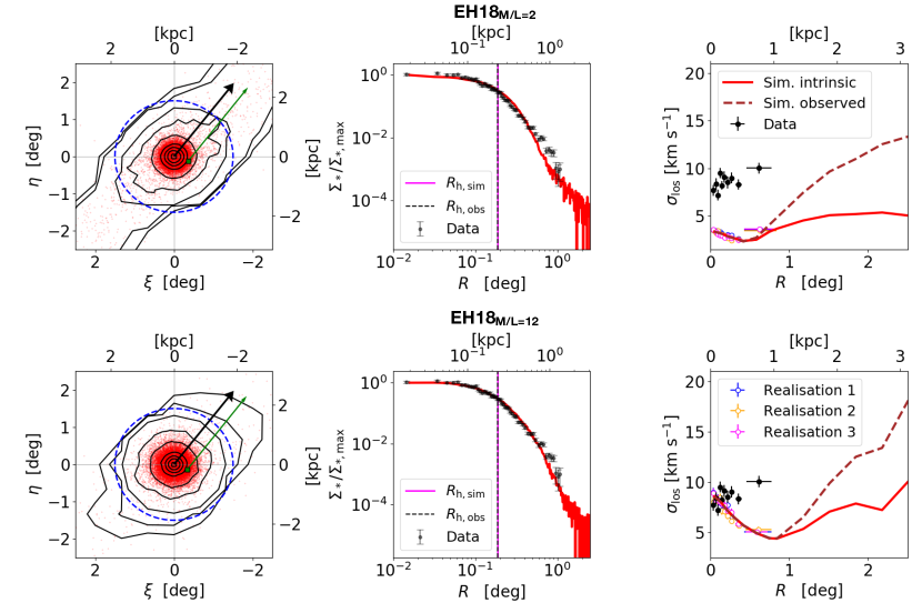
Figure 10: Same as Fig. 7, but for the last snapshot of the last-iteration simulation of the EH18 mass-follows-light model (see text) considering a baryonic mass-to-light ratio $\Upsilon_{*}=2$ (upper panels) and $\Upsilon_{*}=12$ (lower panels).

7 Discussion and conclusions

In this work, we used ad-hoc $N$-body simulations to analyse the dynamical evolution of the Sculptor dSph in the tidal field of the MW. The dynamical models of the satellite and its backward orbits have been based on state-of-the-art observational data (see Sec. 2). Our final simulations are able to nicely reproduce the current position and velocities of Sculptor as well as the observed angle-averaged los surface density and velocity dispersion profile. The results of this work (Sec. 6) indicate that, even considering one of the most eccentric orbit allowed by the data uncertainties (primarily on the proper motions but also on other quantities; see Sec. 3.2), the direct effects of tides on the baryonic content of the satellite are negligible, and no significant tidal tails are developed. Even if not directly affected by tides, the stellar component of the satellite shows a certain degree of evolution because of the response to the significant mass loss experienced by the more extended DM halo. In particular, the half-light radius increases and the velocity dispersion decreases. However, in the last 2 Gyr the evolution proceeds very slowly, the structural and kinematic parameters of the baryonic component change less than about 5% and the satellite in the last snapshots is close to equilibrium in its own gravitational potential. These results suggest that the assumption of dynamical equilibrium can be safely used to estimate the dynamical mass of Sculptor (Sec. 6.3). Moreover the lack of stellar tidal tails in the simulations indicates that we can consider the existing kinematic samples free from contamination by tidally stripped stars. These results are similar to what obtained by Battaglia et al. (2015) for the Fornax dSph and they are compatible with the results of Peñarrubia et al. (2009a).

Recently Hammer et al. (2018b) suggested that the gravitational acceleration due to the MW could heavily affect the los velocity dispersion of satellites. In classical dSphs, such as Sculptor, this could explain the observed high los velocity dispersion (Hammer et al., 2018a). Since this is a purely gravitational effect, its imprint should be present in our simulations. However, we found that in all our simulations, either including an extended DM halo (Sec. 6.2) or assuming a mass-follows-light model (Sec. 6.4), the evolution of the los velocity dispersion profile within the observed range is driven by the mass loss of the DM halo and/or the property of the baryonic component. This is evident also in the mass-follows-light models: the right-hand panels of Fig. 10 show that at the half-light radius the los velocity dispersion is totally determined by the distribution of matter inside the galaxy (in both shape and magnitude).

The simulations that successfully reproduce Sculptor’s observables have dark-to-luminous mass ratios 5.9 (FH18₁₄) and 5.4 (EH18₁₇) within the projected stellar half-mass radius (283 pc in FH18₁₄ and 271 pc in EH18₁₇) and 62.1 (FH18₁₄) and 55.9 (EH18₁₇) within the projected $R_{*}=1.5^{\circ}$ radius (2.25 kpc in FH18₁₄ and 2.16 kpc in EH18₁₇). The loss of DM is substantial: the initial mass of the satellite was at least two (FH18₁₄) and up to four (EH18₁₇) times higher 7 Gyr ago than today.

The results of this work are based on a number of working assumptions. Most of them are simplifications that we tuned with the idea to maximise the possible tidal effects. First of all, we used a time-independent external potential considering a “fully grown” MW for the entire $\approx 7\ \text{Gyr}$ of the orbital evolution. The used potential is a simple analytic model J95 that represents a “heavy” MW ($M_{200}>2\times 10^{12}\ \,{\rm M}_{\odot}$, see Sec. 3.1). Although this model does not represent the state of the art of the dynamical modelling of the MW and it does not take into account the hierarchical mass evolution of the Galaxy, it maximises the influence of tides on Sculptor. Therefore, our results are robust in the sense that if the tidal effects are not important in the analysed case it is likely that this holds even considering more sophisticated and time-dependent MW potential models.

Concerning the assumption of the Sculptor’s orbit, we relied on the robust estimate of the proper motions given by $Gaia$ (H18, F18). However the reported formal errors do not take into account the $Gaia$ systematics (Lindegren et al., 2018). An estimate of the large scale systematic error can be obtained using Eq. 18 in Lindegren et al. (2018). For the $\approx 1^{\circ}$ degree area analysed in H18 we get $\delta_{\mu,\text{sys}}\approx 0.028$ mas yr^-1 (see Tab. 3.1). In addition, we repeated the H18 orbital investigation (Sec. 5.2.1) using the larger systematic error ($\delta_{\mu,\text{sys}}\approx 0.066$ mas yr^-1) reported in Lindegren et al. (2018) for small angular scales. Increasing the proper motion error, the distribution of the pericentre radius becomes wider and the $3\sigma$ lower limit decreases to $\approx 23$ kpc, while the pericentre of our most eccentric analysed orbit (EH18, see Tab. 3) is contained within $2\sigma$. We applied our iterative method considering a new extreme orbit with $r_{\text{peri}}=23$ kpc and we found that in this case the tides are strong enough to influence significantly also the baryonic component of the dwarf. The final results are very similar to the mass-follows-light models analysed in Sec. 6.4, the significant mass loss causes a strong decrease of the velocity dispersion ($\sigma_{\text{los}}\approx 5\ \,{\rm km\,s}^{-1}$) that does not match the observed kinematics. Although our method is able to explore only a limited portion of the dwarf initial conditions, our analysis points out that considering a highly eccentric orbit ($e>0.6$) it is challenging to reproduce the observed Sculptor’s properties. It is also important to notice that in our analysis, we did not take into account the presence of the Large Magellanic Cloud (LMC). This massive object ($\approx 10^{11}\,{\rm M}_{\odot}$, Erkal et al. 2018) could significantly perturb the MW satellites orbits. S17 explored this effect finding that the LMC perturbation tends on one side to decrease the pericentric radius and on the other side to increase the orbital period. However, even in the extreme case of a very massive MW ($M_{MW}=2\times 10^{12}\ \,{\rm M}_{\odot}$) and very massive LMC ($M_{MW}=2.5\times 10^{11}\ \,{\rm M}_{\odot}$), the pericentre found by S17 ($\approx 40\ \,{\rm kpc}$) is larger than what we have analysed with the EH18 orbit ($r_{\text{peri}}\approx 36\ \,{\rm kpc}$, see Sec. 3.2). Therefore, considering the results of this work (Sec. 6), it is unlikely that the LMC has produced any significant tidal effect on the baryonic component of Sculptor. However, in the future, it will be interesting to investigate further and in greater details the influence of the LMC on the dynamics and kinematics of Sculptor and other MW satellites.

The dynamical models that we used for the dark matter halo of the simulated satellites rely on the present-day ($z=0$) concentration-mass relation (Sec. 4.1.2). However, the assumed simulation times ($t_{\text{sim}}\approx 7$ Gyr, see Tab. 4) correspond to an initial redshift $z\approx 0.8$. At that redshift, the concentration parameter expected for the halo mass range analysed in this work can be as low as 9. However, most of this evolution is, in fact, a pseudo-evolution driven by the change of critical density of the Universe (Diemer & Joyce, 2019). In practice, at given $r_{\text{c}}$ and $M_{200}$ the density profiles based on the $c_{200}$-$M_{200}$ relations at $z=0$ and $z=0.8$ are very similar. As an additional check, we repeated the dynamical fitting of los velocity distribution (Sec. 4.2) and we ran the simulation EH18₁₇ (Sec. 5) assuming the $c_{200}$-$M_{200}$ relation at $z=0.8$ (Diemer & Joyce, 2019). We found that the final results are largely consistent with what we found assuming $z=0$ (Sec. 6).

Another fundamental assumption is that we consider only spherical and isotropic models. In Sec. 4, we demonstrated that an isotropic model with a cored DM halo can give a reasonable fit to observed los velocity distributions of Sculptor. Using a cored DM halo we maximised the effect of tides since the baryonic component is less “shielded” from tides with respect to a cuspy halo profile (Peñarrubia et al., 2008, 2010; Frings et al., 2017). Concerning the shape of the baryonic distribution, we assumed for simplicity a spherical distribution, in order to limit the number of degrees of freedoms. However, in a work analogous to the present one, but for the Fornax dSphs, Battaglia et al. (2015), found that the results do not change when a flattened model is used instead of a spherical one. Given the similarity of the method and of the results of the two works, we are confident that the inclusion of a more sophisticated flattened model does not affect the main conclusions of our work.

In the present work, we do not attempt a detailed study of the internal dynamics of Sculptor and we make a few simplifying assumptions. In particular, when we build the dynamical model (Sec. 4), we assume a single stellar population and isotropic velocity distribution. The most restrictive assumption is the assumption of isotropy. Considering two stellar populations would be useful only if they were allowed to be anisotropic. About the velocity distribution, our assumption is conservative: if we had assumed radial anisotropy (as indicated by previous works on the internal dynamics of Sculptor, see e.g. Battaglia et al. 2008; Massari et al. 2018), the DM halo would have been more massive than in the isotropic case and thus the tidal effects even milder than found in our simulations. However, we stress that the DM halo assumed in our model, though derived under simplifying assumptions, is not unrealistic. For instance, Pascale et al. (2019), allowing for the presence of two anisotropic stellar components, find that Sculptor is well modelled with a DM halo very similar to ours.

The last key assumption is about the use of “dry” simulations without a gaseous component. Since we analysed the satellite evolution over the last $\approx 7\ \text{Gyr}$, the SFH of Sculptor justifies this assumption (de Boer et al., 2012; Bermejo-Climent et al., 2018). Although the use of more sophisticated hydrodynamic simulations could allow us to explore more realistic initial conditions for the satellite (Mayer et al., 2006; Nichols & Bland-Hawthorn, 2011; Kazantzidis et al., 2017; Hammer et al., 2018a), the results of the present work suggest that, in the presence of an extended DM halo, it is difficult that significant tidal perturbations develop in the stellar component of Sculptor.

In conclusion, we would like to stress again that the use of ad-hoc $N$-body simulations, such as those presented here, is a valuable tool to complement the dynamical analysis of MW satellites. Only in this way, it is possible to explore in details the possible perturbations produced by the MW tidal field and verify the validity of equilibrium models. The release of Gaia data and of the forthcoming large surveys make it possible to have robust proper motion estimates not only for classical dSph satellites but also for ultrafaint and low surface brightness dwarfs (e.g. Crater 2, Torrealba et al. 2016; Caldwell et al. 2017; or Antlia 2, Torrealba et al. 2018). The investigation of the properties of these objects with $N$-body simulations based on realistic orbits is a fundamental step in the attempt to understand their content of DM and their formation and evolution (see e.g. Sanders et al. 2018).

Acknowledgements

The authors thank Raffaele Pascale for useful discussions and Luis Cicuéndez for the analysis of the light distribution of Sculptor. We thank the anonymous referee for suggestions that helped to improve this manuscript. In this work we made use of the Python modules matplotlib (Hunter, 2007), numpy and scipy (Jones et al., 01). We also made use of the comology calculator by Wright (2006). G.I. is supported by the Royal Society Newton International Fellowship (NF170902). G.B. gratefully acknowledges financial support from Spanish Ministry of Economy and Competitivness (MINECO) under the Ramon y Cajal Programme (RYC-2012-11537) and the grant AYA2017-89076-P.

Appendix A Mock observations

In order to compare the final snapshot of the simulations with the observations of Sculptor, we simulate the observation of the stellar particles projecting them on the sky plane. The procedure consist in the following steps. (i) We modify the positions of the particles from the Galactocentric frame of reference (see Sec. 3.1) to a right-handed heliocentric frame of reference. In practice, we translate the original frame of reference by $R_{\odot}$ along the $x$-axis and then we switch the direction of the $x$-axis, so that it points towards the Galactic centre. (ii) Given the positions of the particles with respect to the Sun we estimate the sky coordinates and we set the central coordinates of our simulated object as the sky coordinate of its COS (see Sec. 5.3). (iii) We add to the particle velocities the extra components $-\vec{v}_{\odot}$ due to the motion of the Sun in the inertial Galactic frame of reference (see Tab. 3). (iv) Finally, for each stellar particle we apply a rotoreflection (combination of a rotation and a reflection in a plane perpendicular to one of the rotation axes) of the heliocentric frame of reference, so that the new $z$-axis is the line connecting the Sun with the stars, the $x$-axis points toward the Galactic South-Cap and the $y$-axis is aligned with the Galactic longitude:

$$\begin{bmatrix}V_{b}&V_{\ell}&V_{\text{los}}\end{bmatrix}=\begin{bmatrix}V_{x}&V_{y}&V_{z}\end{bmatrix}\textbf{{R}}_{\text{rot}},$$ (15)

where

$$\textbf{{R}}_{\text{rot}}=\begin{bmatrix}-\cos(\ell)\sin(b)&-\sin(\ell)&\cos(\ell)\sin(b)\\ -\sin(\ell)\sin(b)&\cos(\ell)&\sin(\ell)\cos(b)\\ \cos(b)&0&\sin(b)\end{bmatrix}.$$ (16)

In this new frame of reference, the velocity along the $z$-axis is the observed $V_{\text{los}}$, while the velocities along the $x$ and $y$ axes represent the velocities $V_{b}$, $V_{\ell}$ along the Galactic latitude and longitude, respectively. Once we have all the coordinates and the velocity in the Galactic sky coordinates, we use the classical geometrical transformation to obtain also the same information in the equatorial sky coordinate system (Johnson & Soderblom, 1987). After this procedure, we obtain the sky position of the centre of the simulated object as well as the observed properties (sky-position, radial velocity and proper motion) for each stellar particle in the snapshot.

References

- Aaronson (1983) Aaronson M., 1983, ApJ, 266, L11
- Amorisco & Evans (2012) Amorisco N. C., Evans N. W., 2012, MNRAS, 419, 184
- Anderhalden et al. (2013) Anderhalden D., Schneider A., Macciò A. V., Diemand J., Bertone G., 2013, J. Cosmology Astropart. Phys., 3, 014
- Battaglia & Starkenburg (2012) Battaglia G., Starkenburg E., 2012, A&A, 539, A123
- Battaglia et al. (2005) Battaglia G., et al., 2005, MNRAS, 364, 433
- Battaglia et al. (2008) Battaglia G., Helmi A., Tolstoy E., Irwin M., Hill V., Jablonka P., 2008, ApJ, 681, L13
- Battaglia et al. (2011) Battaglia G., Tolstoy E., Helmi A., Irwin M., Parisi P., Hill V., Jablonka P., 2011, MNRAS, 411, 1013
- Battaglia et al. (2013) Battaglia G., Helmi A., Breddels M., 2013, New Astron. Rev., 57, 52
- Battaglia et al. (2015) Battaglia G., Sollima A., Nipoti C., 2015, MNRAS, 454, 2401
- Baumgardt & Makino (2003) Baumgardt H., Makino J., 2003, MNRAS, 340, 227
- Belokurov et al. (2018) Belokurov V., Erkal D., Evans N. W., Koposov S. E., Deason A. J., 2018, MNRAS, 478, 611
- Bermejo-Climent et al. (2018) Bermejo-Climent J. R., et al., 2018, MNRAS, 479, 1514
- Binney & Tremaine (2008) Binney J., Tremaine S., 2008, Galactic Dynamics: Second Edition. Princeton University Press
- Bovy (2014) Bovy J., 2014, ApJ, 795, 95
- Bovy (2015) Bovy J., 2015, ApJS, 216, 29
- Bovy et al. (2011) Bovy J., Hogg D. W., Roweis S. T., 2011, Annals of Applied Statistics, 5
- Bovy et al. (2012) Bovy J., et al., 2012, ApJ, 759, 131
- Boylan-Kolchin et al. (2011) Boylan-Kolchin M., Bullock J. S., Kaplinghat M., 2011, MNRAS, 415, L40
- Breddels & Helmi (2013) Breddels M. A., Helmi A., 2013, A&A, 558, A35
- Breddels & Helmi (2014) Breddels M. A., Helmi A., 2014, ApJ, 791, L3
- Bullock et al. (2000) Bullock J. S., Kravtsov A. V., Weinberg D. H., 2000, ApJ, 539, 517
- Caldwell et al. (2017) Caldwell N., et al., 2017, ApJ, 839, 20
- Cicuéndez et al. (2018) Cicuéndez L., et al., 2018, A&A, 609, A53
- Contigiani et al. (2018) Contigiani O., Rossi E. M., Marchetti T., 2018, preprint, (arXiv:1807.04468)
- Dabringhausen et al. (2016) Dabringhausen J., Kroupa P., Famaey B., Fellhauer M., 2016, MNRAS, 463, 1865
- Dale et al. (2009) Dale D. A., et al., 2009, ApJ, 703, 517
- Deason et al. (2012) Deason A. J., Belokurov V., Evans N. W., An J., 2012, MNRAS, 424, L44
- Diemer (2017) Diemer B., 2017, arXiv e-prints, p. arXiv:1712.04512
- Diemer & Joyce (2019) Diemer B., Joyce M., 2019, ApJ, 871, 168
- Duquennoy & Mayor (1991) Duquennoy A., Mayor M., 1991, A&A, 248, 485
- Erkal et al. (2018) Erkal D., et al., 2018, arXiv e-prints, p. arXiv:1812.08192
- Errani et al. (2018) Errani R., Peñarrubia J., Walker M. G., 2018, MNRAS, 481, 5073
- Fattahi et al. (2018) Fattahi A., Navarro J. F., Frenk C. S., Oman K. A., Sawala T., Schaller M., 2018, MNRAS, 476, 3816
- Feigelson & Babu (2012) Feigelson E. D., Babu G. J., 2012, Modern Statistical Methods for Astronomy
- Ferguson & Binggeli (1994) Ferguson H. C., Binggeli B., 1994, A&ARv, 6, 67
- Fleck & Kuhn (2003) Fleck J.-J., Kuhn J. R., 2003, ApJ, 592, 147
- Foreman-Mackey et al. (2013) Foreman-Mackey D., Hogg D. W., Lang D., Goodman J., 2013, PASP, 125, 306
- Frings et al. (2017) Frings J., Macciò A., Buck T., Penzo C., Dutton A., Blank M., Obreja A., 2017, MNRAS, 472, 3378
- Fritz et al. (2018) Fritz T. K., Battaglia G., Pawlowski M. S., Kallivayalil N., van der Marel R., Sohn T. S., Brook C., Besla G., 2018, preprint, (arXiv:1805.00908)
- Gaia Collaboration et al. (2016) Gaia Collaboration et al., 2016, A&A, 595, A1
- Gaia Collaboration et al. (2018b) Gaia Collaboration et al., 2018b, preprint, (arXiv:1804.09381)
- Gaia Collaboration et al. (2018a) Gaia Collaboration Brown A. G. A., Vallenari A., Prusti T., de Bruijne J. H. J., Babusiaux C., Bailer-Jones C. A. L., 2018a, preprint, (arXiv:1804.09365)
- Garofalo et al. (2018) Garofalo A., et al., 2018, preprint, (arXiv:1808.04843)
- Gerhard (1993) Gerhard O. E., 1993, MNRAS, 265, 213
- Gibbons et al. (2014) Gibbons S. L. J., Belokurov V., Evans N. W., 2014, MNRAS, 445, 3788
- Gilmore et al. (2007) Gilmore G., Wilkinson M. I., Wyse R. F. G., Kleyna J. T., Koch A., Evans N. W., Grebel E. K., 2007, ApJ, 663, 948
- Grebel et al. (2003) Grebel E. K., Gallagher III J. S., Harbeck D., 2003, AJ, 125, 1926
- Hammer et al. (2018a) Hammer F., Yang Y., Wang J., Arenou F., Puech M., Flores H., 2018a, arXiv e-prints, p. arXiv:1812.10714
- Hammer et al. (2018b) Hammer F., Yang Y., Arenou F., Babusiaux C., Wang J., Puech M., Flores H., 2018b, ApJ, 860, 76
- Hargreaves et al. (1996) Hargreaves J. C., Gilmore G., Annan J. D., 1996, MNRAS, 279, 108
- Helmi et al. (2018) Helmi A., Babusiaux C., Koppelman H. H., Massari D., Veljanoski J., Brown A. G. A., 2018, preprint, (arXiv:1806.06038)
- Hernquist (1990) Hernquist L., 1990, ApJ, 356, 359
- Hunter (2007) Hunter J. D., 2007, Computing In Science & Engineering, 9, 90
- Johnson & Soderblom (1987) Johnson D. R. H., Soderblom D. R., 1987, AJ, 93, 864
- Johnston et al. (1995) Johnston K. V., Spergel D. N., Hernquist L., 1995, ApJ, 451, 598
- Jones et al. (01 ) Jones E., Oliphant T., Peterson P., et al., 2001–, SciPy: Open source scientific tools for Python, http://www.scipy.org/
- Kazantzidis et al. (2017) Kazantzidis S., Mayer L., Callegari S., Dotti M., Moustakas L. A., 2017, ApJ, 836, L13
- Kennedy et al. (2014) Kennedy R., Frenk C., Cole S., Benson A., 2014, MNRAS, 442, 2487
- Kleyna et al. (2002) Kleyna J., Wilkinson M. I., Evans N. W., Gilmore G., Frayn C., 2002, MNRAS, 330, 792
- Klimentowski et al. (2007) Klimentowski J., Łokas E. L., Kazantzidis S., Prada F., Mayer L., Mamon G. A., 2007, MNRAS, 378, 353
- Klimentowski et al. (2009) Klimentowski J., Łokas E. L., Kazantzidis S., Mayer L., Mamon G. A., Prada F., 2009, MNRAS, 400, 2162
- Klypin et al. (1999) Klypin A., Kravtsov A. V., Valenzuela O., Prada F., 1999, ApJ, 522, 82
- Koch et al. (2007) Koch A., Kleyna J. T., Wilkinson M. I., Grebel E. K., Gilmore G. F., Evans N. W., Wyse R. F. G., Harbeck D. R., 2007, AJ, 134, 566
- Koposov et al. (2011) Koposov S. E., et al., 2011, ApJ, 736, 146
- Kroupa (1997) Kroupa P., 1997, New Astron., 2, 139
- Kruijssen et al. (2018) Kruijssen J. M. D., Pfeffer J. L., Reina-Campos M., Crain R. A., Bastian N., 2018, MNRAS,
- Kubik et al. (2017) Kubik B., Libeskind N. I., Knebe A., Courtois H., Yepes G., Gottlöber S., Hoffman Y., 2017, MNRAS, 472, 4099
- Li & White (2008) Li Y.-S., White S. D. M., 2008, MNRAS, 384, 1459
- Lindegren et al. (2018) Lindegren L., et al., 2018, preprint, (arXiv:1804.09366)
- Londrillo et al. (2003) Londrillo P., Nipoti C., Ciotti L., 2003, Memorie della Societa Astronomica Italiana Supplementi, 1, 18
- Macciò & Fontanot (2010) Macciò A. V., Fontanot F., 2010, MNRAS, 404, L16
- Mamon & Łokas (2005) Mamon G. A., Łokas E. L., 2005, MNRAS, 363, 705
- Martínez-Vázquez et al. (2015) Martínez-Vázquez C. E., et al., 2015, MNRAS, 454, 1509
- Massari et al. (2018) Massari D., Breddels M. A., Helmi A., Posti L., Brown A. G. A., Tolstoy E., 2018, Nature Astronomy, 2, 156
- Mateo (1998) Mateo M. L., 1998, ARA&A, 36, 435
- Mateo et al. (1993) Mateo M., Olszewski E. W., Pryor C., Welch D. L., Fischer P., 1993, AJ, 105, 510
- Mateo et al. (2008) Mateo M., Olszewski E. W., Walker M. G., 2008, ApJ, 675, 201
- Mayer (2011) Mayer L., 2011, in Koleva M., Prugniel P., Vauglin I., eds, EAS Publications Series Vol. 48, EAS Publications Series. pp 369–381 (arXiv:1104.4278), doi:10.1051/eas/1148085
- Mayer et al. (2006) Mayer L., Mastropietro C., Wadsley J., Stadel J., Moore B., 2006, MNRAS, 369, 1021
- McConnachie (2012) McConnachie A. W., 2012, AJ, 144, 4
- Menzies et al. (2011) Menzies J. W., Feast M. W., Whitelock P. A., Matsunaga N., 2011, MNRAS, 414, 3492
- Metz & Kroupa (2007) Metz M., Kroupa P., 2007, MNRAS, 376, 387
- Minor (2013) Minor Q. E., 2013, ApJ, 779, 116
- Miyamoto & Nagai (1975) Miyamoto M., Nagai R., 1975, PASJ, 27, 533
- Monari et al. (2018) Monari G., et al., 2018, preprint, (arXiv:1807.04565)
- Moore et al. (1999) Moore B., Ghigna S., Governato F., Lake G., Quinn T., Stadel J., Tozzi P., 1999, ApJ, 524, L19
- Muñoz et al. (2006a) Muñoz R. R., et al., 2006a, ApJ, 649, 201
- Muñoz et al. (2006b) Muñoz R. R., Carlin J. L., Frinchaboy P. M., Nidever D. L., Majewski S. R., Patterson R. J., 2006b, ApJ, 650, L51
- Muñoz et al. (2008) Muñoz R. R., Majewski S. R., Johnston K. V., 2008, ApJ, 679, 346
- Myeong et al. (2018) Myeong G. C., Evans N. W., Belokurov V., Sanders J. L., Koposov S. E., 2018, preprint, (arXiv:1805.00453)
- Navarro et al. (1996) Navarro J. F., Frenk C. S., White S. D. M., 1996, ApJ, 462, 563
- Nichols & Bland-Hawthorn (2011) Nichols M., Bland-Hawthorn J., 2011, ApJ, 732, 17
- Nipoti & Binney (2015) Nipoti C., Binney J., 2015, MNRAS, 446, 1820
- Nipoti et al. (2003) Nipoti C., Londrillo P., Ciotti L., 2003, MNRAS, 342, 501
- Olszewski et al. (1996) Olszewski E. W., Pryor C., Armandroff T. E., 1996, AJ, 111, 750
- Pascale et al. (2018) Pascale R., Posti L., Nipoti C., Binney J., 2018, MNRAS, 480, 927
- Pascale et al. (2019) Pascale R., Binney J., Nipoti C., Posti L., 2019, preprint, (arXiv:1904.08447)
- Peñarrubia et al. (2008) Peñarrubia J., Navarro J. F., McConnachie A. W., 2008, ApJ, 673, 226
- Peñarrubia et al. (2009a) Peñarrubia J., Navarro J. F., McConnachie A. W., Martin N. F., 2009a, ApJ, 698, 222
- Peñarrubia et al. (2009b) Peñarrubia J., Navarro J. F., McConnachie A. W., Martin N. F., 2009b, ApJ, 698, 222
- Peñarrubia et al. (2010) Peñarrubia J., Benson A. J., Walker M. G., Gilmore G., McConnachie A. W., Mayer L., 2010, MNRAS, 406, 1290
- Piatek et al. (2006) Piatek S., Pryor C., Bristow P., Olszewski E. W., Harris H. C., Mateo M., Minniti D., Tinney C. G., 2006, AJ, 131, 1445
- Pietrzyński et al. (2008) Pietrzyński G., et al., 2008, AJ, 135, 1993
- Piffl et al. (2014) Piffl T., et al., 2014, MNRAS, 445, 3133
- Planck Collaboration et al. (2016) Planck Collaboration et al., 2016, A&A, 594, A13
- Pontzen & Governato (2012) Pontzen A., Governato F., 2012, MNRAS, 421, 3464
- Posti & Helmi (2018) Posti L., Helmi A., 2018, preprint, (arXiv:1805.01408)
- Power et al. (2003) Power C., Navarro J. F., Jenkins A., Frenk C. S., White S. D. M., Springel V., Stadel J., Quinn T., 2003, MNRAS, 338, 14
- Read et al. (2006) Read J. I., Wilkinson M. I., Evans N. W., Gilmore G., Kleyna J. T., 2006, MNRAS, 366, 429
- Read et al. (2016) Read J. I., Agertz O., Collins M. L. M., 2016, MNRAS, 459, 2573
- Read et al. (2017) Read J. I., Iorio G., Agertz O., Fraternali F., 2017, MNRAS, 467, 2019
- Read et al. (2018) Read J. I., Walker M. G., Steger P., 2018, MNRAS, 481, 860
- Rizzi et al. (2007) Rizzi L., Tully R. B., Makarov D., Makarova L., Dolphin A. E., Sakai S., Shaya E. J., 2007, ApJ, 661, 815
- Salaris et al. (2013) Salaris M., de Boer T., Tolstoy E., Fiorentino G., Cassisi S., 2013, A&A, 559, A57
- Sanders et al. (2018) Sanders J. L., Evans N. W., Dehnen W., 2018, MNRAS, 478, 3879
- Schönrich (2012) Schönrich R., 2012, MNRAS, 427, 274
- Schweitzer et al. (1995) Schweitzer A. E., Cudworth K. M., Majewski S. R., Suntzeff N. B., 1995, AJ, 110, 2747
- Sohn et al. (2007) Sohn S. T., et al., 2007, ApJ, 663, 960
- Sohn et al. (2017) Sohn S. T., et al., 2017, ApJ, 849, 93
- Spencer et al. (2018) Spencer M. E., Mateo M., Olszewski E. W., Walker M. G., McConnachie A. W., Kirby E. N., 2018, AJ, 156, 257
- Starkenburg et al. (2010) Starkenburg E., et al., 2010, A&A, 513, A34
- Strigari et al. (2017) Strigari L. E., Frenk C. S., White S. D. M., 2017, ApJ, 838, 123
- Strigari et al. (2018) Strigari L. E., Frenk C. S., White S. D. M., 2018, ApJ, 860, 56
- Takahashi & Lee (2000) Takahashi K., Lee H. M., 2000, MNRAS, 316, 671
- Tolstoy (2014) Tolstoy E., 2014, in Feltzing S., Zhao G., Walton N. A., Whitelock P., eds, IAU Symposium Vol. 298, Setting the scene for Gaia and LAMOST. pp 53–58, doi:10.1017/S1743921313006194
- Tolstoy et al. (2004) Tolstoy E., et al., 2004, ApJ, 617, L119
- Torrealba et al. (2016) Torrealba G., Koposov S. E., Belokurov V., Irwin M., 2016, MNRAS, 459, 2370
- Torrealba et al. (2018) Torrealba G., et al., 2018, arXiv e-prints, p. arXiv:1811.04082
- Ural et al. (2015) Ural U., Wilkinson M. I., Read J. I., Walker M. G., 2015, Nature Communications, 6, 7599
- Walker (2013) Walker M., 2013, Dark Matter in the Galactic Dwarf Spheroidal Satellites. p. 1039, doi:10.1007/978-94-007-5612-0_20
- Walker & Peñarrubia (2011) Walker M. G., Peñarrubia J., 2011, ApJ, 742, 20
- Walker et al. (2008) Walker M. G., Mateo M., Olszewski E. W., 2008, ApJ, 688, L75
- Walker et al. (2009a) Walker M. G., Mateo M., Olszewski E. W., 2009a, AJ, 137, 3100
- Walker et al. (2009b) Walker M. G., Mateo M., Olszewski E. W., Peñarrubia J., Wyn Evans N., Gilmore G., 2009b, ApJ, 704, 1274
- Wang et al. (2015) Wang W., Han J., Cooper A. P., Cole S., Frenk C., Lowing B., 2015, MNRAS, 453, 377
- Weisz et al. (2014) Weisz D. R., Dolphin A. E., Skillman E. D., Holtzman J., Gilbert K. M., Dalcanton J. J., Williams B. F., 2014, ApJ, 789, 147
- Wilkinson & Evans (1999) Wilkinson M. I., Evans N. W., 1999, MNRAS, 310, 645
- Woo et al. (2008) Woo J., Courteau S., Dekel A., 2008, Monthly Notices of the Royal Astronomical Society, 390, 1453
- Wright (2006) Wright E. L., 2006, PASP, 118, 1711
- Xue et al. (2008) Xue X. X., et al., 2008, ApJ, 684, 1143
- Zhu et al. (2016) Zhu L., van de Ven G., Watkins L. L., Posti L., 2016, MNRAS, 463, 1117
- de Boer et al. (2012) de Boer T. J. L., et al., 2012, A&A, 539, A103
- van der Marel & Franx (1993) van der Marel R. P., Franx M., 1993, ApJ, 407, 525