An Interior Point-Proximal Method of Multipliers for Convex Quadratic Programming

Abstract

In this paper we combine an infeasible Interior Point Method (IPM) with the Proximal Method of Multipliers (PMM). The resulting algorithm (IP-PMM) is interpreted as a primal-dual regularized IPM, suitable for solving linearly constrained convex quadratic programming problems. We apply few iterations of the interior point method to each sub-problem of the proximal method of multipliers. Once a satisfactory solution of the PMM sub-problem is found, we update the PMM parameters, form a new IPM neighbourhood and repeat this process. Given this framework, we prove polynomial complexity of the algorithm, under standard assumptions. To our knowledge, this is the first polynomial complexity result for a primal-dual regularized IPM. The algorithm is guided by the use of a single penalty parameter; that of the logarithmic barrier. In other words, we show that IP-PMM inherits the polynomial complexity of IPMs, as well as the strict convexity of the PMM sub-problems. The updates of the penalty parameter are controlled by IPM, and hence are well-tuned, and do not depend on the problem solved. Furthermore, we study the behavior of the method when it is applied to an infeasible problem, and identify a necessary condition for infeasibility. The latter is used to construct an infeasibility detection mechanism. Subsequently, we provide a robust implementation of the presented algorithm and test it over a set of small to large scale linear and convex quadratic programming problems. The numerical results demonstrate the benefits of using regularization in IPMs as well as the reliability of the method.

1 Introduction

Primal-Dual Pair of Convex Quadratic Programming Problems

In this paper, we consider the following primal-dual pair of linearly constrained convex quadratic programming problems, in the standard form:

$$\text{min}_{x}\ \big{(}c^{T}x+\frac{1}{2}x^{T}Qx\big{)},\ \ \text{s.t.}\ Ax=b,\ x\geq 0,$$ (P)

$$\text{max}_{x,y,z}\ \big{(}b^{T}y-\frac{1}{2}x^{T}Qx\big{)},\ \ \text{s.t.}\ -Qx+A^{T}y+z=c,\ z\geq 0,$$ (D)

with $c,x,z\in\mathbb{R}^{n}$, $b,y\in\mathbb{R}^{m}$, $A\in\mathbb{R}^{m\times n}$, and symmetric positive semi-definite $Q\in\mathbb{R}^{n\times n}$ (i.e. $Q\succeq 0$). Without loss of generality we assume that $m\leq n$. Duality, between the problems (P)-(D), arises by introducing the Lagrangian function of the primal, using $y\in\mathbb{R}^{m}$ and $z\in\mathbb{R}^{n},\ z\geq 0$, as the Lagrange multipliers for the equality and inequality constraints, respectively. Hence, we obtain:

$$\mathcal{L}(x,y,z)=c^{T}x+\frac{1}{2}x^{T}Qx-y^{T}(Ax-b)-z^{T}x.$$ (1.1)

Using the Lagrangian function, one can formulate the first-order optimality conditions (known as Karush–Kuhn–Tucker (KKT) conditions) for this primal-dual pair. In particular, we define the vector $w=(x^{T},y^{T},z^{T})^{T}$, and compute the gradient of $\mathcal{L}(w)$. Using $\nabla\mathcal{L}(w)$, as well as the complementarity conditions, we may define a function $F(w):\mathbb{R}^{2n+m}\mapsto\mathbb{R}^{2n+m}$, using which, we write the KKT conditions as follows:

$$F(w)=\begin{bmatrix}c+Qx-A^{T}y-z\\ Ax-b\\ XZe_{n}\\ \end{bmatrix}=\begin{bmatrix}0\\ 0\\ 0\\ \end{bmatrix},\qquad(x,z)\geq(0,0),$$ (1.2)

where $e_{n}$ denotes the vector of ones of size $n$, while $X,\ Z\in\mathbb{R}^{n\times n}$ denote the diagonal matrices satisfying $X^{ii}=x^{i}$ and $Z^{ii}=z^{i}$, $\forall\ i\in\{1,\cdots,n\}$. For the rest of this manuscript, superscripts will denote the components of a vector/matrix. For simplicity of exposition, when referring to convex quadratic programming problems, we implicitly assume that the problems are linearly constrained. If both (P) and (D) are feasible problems, it can easily be verified that there exists an optimal primal-dual triple $(x,y,z)$, satisfying the KKT optimality conditions of this primal-dual pair (see for example in [7, Prop. 2.3.4]).

A Primal-Dual Interior Point Method

Primal-dual Interior Point Methods (IPMs) are popular for simultaneously solving (P) and (D), iteratively. As indicated in the name, primal-dual IPMs act on both primal and dual variables. There are numerous variants of IPMs and the reader is referred to [16] for an extended literature review. In this paper, an infeasible primal-dual IPM is presented. Such methods are called infeasible because they allow intermediate iterates of the method to be infeasible for (P)-(D), in contrast to feasible IPMs, which require intermediate iterates to be strictly feasible.

Interior point methods handle the non-negativity constraints of the problems with logarithmic barriers in the objective. That is, at each iteration, we choose a barrier parameter $\mu$ and form the logarithmic barrier primal-dual pair:

$$\begin{split}\text{min}_{x}\ \big{(}c^{T}x+\frac{1}{2}x^{T}Qx-\mu\sum_{j=1}^{n}\ln x^{j}\big{)}\ \ \text{s.t.}\ Ax=b,\\ \end{split}$$ (1.3)

$$\begin{split}\text{max}_{x,y,z}\ \big{(}\ b^{T}y-\frac{1}{2}x^{T}Qx+\mu\sum_{j=1}^{n}\ln z^{j}\big{)}\ \ \text{s.t.}\ -Qx+A^{T}y+z=c,\\ \end{split}$$ (1.4)

in which non-negativity constraints $x>0$ and $z>0$ are implicit. We form the KKT optimality conditions of the pair (1.3)-(1.4), by introducing the Lagrangian of the primal barrier problem:

$$\mathcal{L}^{\text{IPM}}_{\mu}(x,y)=c^{T}x+\frac{1}{2}x^{T}Qx-y^{T}(Ax-b)-\mu\sum_{i=1}^{n}\ln x^{j}.$$

Equating the gradient of the previous function to zero, gives the following conditions:

$$\begin{split}\nabla_{x}\mathcal{L}^{\text{IPM}}_{\mu}(x,y)=&\ c+Qx-A^{T}y-\mu X^{-1}e_{n}=0,\\ \nabla_{y}\mathcal{L}^{\text{IPM}}_{\mu}(x,y)=&\ Ax-b=0.\\ \end{split}$$

Using the variable $z=\mu X^{-1}e_{n}$, the final conditions read as follows:

$$\begin{split}c+Qx-A^{T}y-z&=0\\ Ax-b&=0\\ XZe_{n}-\mu e_{n}&=0.\end{split}$$

At each IPM iteration, we want to approximately solve the following mildly non-linear system:

$$F^{\text{IPM}}_{\sigma,\mu}(w)=\begin{bmatrix}c+Qx-A^{T}y-z\\ b-Ax\\ XZe_{n}-\sigma\mu e_{n}\\ \end{bmatrix}=\begin{bmatrix}0\\ 0\\ 0\end{bmatrix},$$ (1.5)

where $F^{\text{IPM}}_{\sigma,\mu}(w)=0$ is a slightly perturbed form of the previously presented optimality conditions. In particular, $\sigma\in(0,1)$ is a centering parameter which determines how fast $\mu$ will be forced to decrease at the next IPM iteration. For $\sigma=1$, we recover the barrier optimality conditions, while for $\sigma=0$ we recover the initial problems’ optimality conditions (1.2). The efficiency of the method depends heavily on the choice of $\sigma$. In fact, various improvements of the traditional IPM schemes have been proposed in the literature, which solve the previous system for multiple carefully chosen values of the centering parameter $\sigma$ and of the right hand side, at each IPM iteration. These are the so called predictor-corrector schemes, proposed for the first time in [22]. Various extensions of such methods have been proposed and analyzed in the literature (e.g. see [15, 34] and references therein). However, for simplicity of exposition, we will follow the traditional approach; $\sigma$ is chosen heuristically at each iteration, and the previous system is solved only once.

In order to approximately solve the system $F^{\text{IPM}}_{\sigma,\mu}(w)=0$ for each value of $\mu$, the most common approach is to apply the Newton method. Newton method is favored for systems of this form, due to the self-concordance of the function $\ln(\cdot)$. For more details on this subject, the interested reader is referred to [24, Chapter 2]. At the beginning of the $k$-th iteration of the IPM, for $k\geq 0$, we have available an iterate $w_{k}=(x_{k}^{T},y_{k}^{T},z_{k}^{T})^{T}$, and a barrier parameter $\mu_{k}$, defined as $\mu_{k}=\frac{x_{k}^{T}z_{k}}{n}$. We choose a value for the centering parameter $\sigma_{k}\in(0,1)$ and form the Jacobian of $F^{\text{IPM}}_{\sigma_{k},\mu_{k}}(\cdot)$, evaluated at $w_{k}$. Then, the Newton direction is determined by solving the following system of equations:

$$\begin{bmatrix}-Q&A^{T}&I\\ A&0&0\\ Z_{k}&0&X_{k}\end{bmatrix}\begin{bmatrix}\Delta x_{k}\\ \Delta y_{k}\\ \Delta z_{k}\end{bmatrix}=-\begin{bmatrix}-c-Qx_{k}+A^{T}y_{k}+z_{k}\\ Ax_{k}-b\\ X_{k}Z_{k}e_{n}-\sigma_{k}\mu_{k}e_{n}\end{bmatrix}.$$ (1.6)

Notice that as $\mu_{k}\rightarrow 0$, the optimal solution of (1.3)-(1.4) converges to the optimal solution of (P)-(D). Polynomial convergence of such methods has been established multiple times in the literature (see for example [35, 36] and the references therein).

Proximal Point Methods

Primal Proximal Point Method

One possible method for solving the primal problem (P), is the so called proximal point method. Given an arbitrary starting point $x_{0}$, the $k$-th iteration of the method is summarized by the following minimization problem:

$$x_{k+1}=\text{arg}\min_{x}\{c^{T}x+\frac{1}{2}x^{T}Qx+\frac{\mu_{k}}{2}\|x-x_{k}\|_{2}^{2},\ \ \text{s.t.}\ Ax=b,\ x\geq 0\},$$

where $\mu_{k}>0$ is a non-increasing sequence of penalty parameters, and $x_{k}$ is the current estimate for an optimal solution of (P) (the use of $\mu_{k}$ is not a mistake; as will become clearer in Section 2, we intend to use the barrier parameter $\mu_{k}$ to control both the IPM and the proximal method). Notice that such an algorithm is not practical, since we have to solve a sequence of sub-problems of similar difficulty to that of (P). Nevertheless, the proximal method contributes the $\mu_{k}I$ term to the Hessian of the objective, and hence the sub-problems are strongly convex. This method is known to achieve a linear convergence rate (and possibly superlinear if $\mu_{k}\rightarrow 0$ at a suitable rate), as shown in [30, 13], among others, even in the case where the minimization sub-problems are solved approximately. Various extensions of this method have been proposed in the literature. For example, one could employ different penalty functions other than the typical 2-norm penalty presented previously (e.g. see [9, 18, 11]).

Despite the fact that such algorithms are not practical, they have served as a powerful theoretical tool and a basis for other important methods. For an extensive review of the applications of standard primal proximal point methods, we refer the reader to [27].

Dual Proximal Point Method

It is a well-known fact, observed for the first time in [30], that the application of the proximal point method on the dual problem, is equivalent to the application of the augmented Lagrangian method on the primal problem, which was proposed for the first time in [17, 29]. In view of the previous fact, we will present the derivation of the augmented Lagrangian method for the primal problem (P), while having in mind that an equivalent reformulation of the model results in the proximal point method for the dual (D) (see [30, 12] or [8, Chapter 3.4.4]).

We start by defining the augmented Lagrangian function of (P). Given an arbitrary starting guess for the dual variables $y_{0}$, the augmented Lagrangian function is defined at the $k$-th iteration as:

$$\mathcal{L}^{\text{ALM}}_{\mu_{k}}(x;y_{k})=c^{T}x+\frac{1}{2}x^{T}Qx-y_{k}^{T}(Ax-b)+\frac{1}{2\mu_{k}}\|Ax-b\|_{2}^{2},$$ (1.7)

where $\mu_{k}>0$ is a non-increasing sequence of penalty parameters and $y_{k}$ is the current estimate of an optimal Lagrange multiplier vector. The augmented Lagrangian method (ALM) is summarized below:

$$\begin{split}x_{k+1}=&\ \text{arg}\min_{x}\{\mathcal{L}^{\text{ALM}}_{\mu_{k}}(x;y_{k}),\ \ \text{s.t.}\ x\geq 0\},\\ y_{k+1}=&\ y_{k}-\frac{1}{\mu_{k}}(Ax_{k+1}-b).\end{split}$$

Notice that the update of the Lagrange multiplier estimates can be interpreted as the application of the dual ascent method. A different type of update would be possible, however, the presented update is cheap and effective, due to the strong concavity of the proximal (“regularized”) dual problem (since $\mu_{k}>0$). Convergence and iteration complexity of such methods have been established multiple times (see for example [30, 20]). There is a vast literature on the subject of augmented Lagrangian methods. For a plethora of technical results and references, the reader is referred to [6]. For convergence results of various extended versions of the method, the reader is referred to [11].

It is worth noting here that a common issue, arising when using augmented Lagrangian methods, is that of the choice of the penalty parameter. To the authors’ knowledge, an optimal tuning for this parameter is still unknown.

Proximal Method of Multipliers

In [30], the author presented, for the first time, the proximal method of multipliers (PMM). The method consists of applying both primal and dual proximal point methods for solving (P)-(D). For an arbitrary starting point $(x_{0},y_{0})$, and using the already defined augmented Lagrangian function, given in (1.7), PMM can be summarized by the following iteration:

$$\begin{split}x_{k+1}=&\ \text{arg}\min_{x}\{\mathcal{L}^{\text{ALM}}_{\mu_{k}}(x;y_{k})+\frac{\mu_{k}}{2}\|x-x_{k}\|_{2}^{2},\ \text{s.t.}\ x\geq 0\},\\ y_{k+1}=&\ y_{k}-\frac{1}{\mu_{k}}(Ax_{k+1}-b),\end{split}$$ (1.8)

where $\mu_{k}$ is a positive non-increasing penalty parameter. One can observe that at every iteration of the method, the primal problem that we have to solve is strongly convex, while its dual, strongly concave. As shown in [30], the addition of the term $\mu_{k}\|x-x_{k}\|_{2}^{2}$, in the augmented Lagrangian method does not affect its convergence rate, while ensuring better numerical behaviour of its iterates. An extension of this algorithm, allowing for the use of more general penalties, can be found in [11].

We can write (1.8) equivalently by making use of the maximal monotone operator $T_{\mathcal{L}}:\mathbb{R}^{n+m}\mapsto\mathbb{R}^{n+m}$ associated to (P)-(D) (see [31, 30]), that is defined as:

$$T_{\mathcal{L}}(x,y)=\{(u,v):v\in Qx+c-A^{T}y+\partial\delta_{+}(x),u=Ax-b\},$$ (1.9)

where $\delta_{+}(\cdot)$ is an indicator function defined as:

$$\delta_{+}(x)=\begin{cases}\infty&\quad\text{if }\exists\ j:x^{j}<0,\\ 0&\quad\text{otherwise.}\\ \end{cases}$$ (1.10)

and $\partial(\cdot)$ denotes the sub-differential of a function. In our case, we have that (see [32, Section 23]):

$$z\in\partial\delta_{+}(x)\Leftrightarrow\begin{cases}z^{j}=0&\text{if }x^{j}>0,\\ z^{j}\leq 0&\text{if }x^{j}=0.\end{cases},\ \forall\ j=\{1,\cdots,n\}.$$

By convention, if there exists a component $j$ such that $x_{j}<0$, we have that $\partial\delta_{+}(x)=\{\emptyset\}$. Given a bounded pair $(x^{*},y^{*})$ such that: $0\in T_{\mathcal{L}}(x^{*},y^{*})$, we can retrieve a vector $z^{*}\in\partial\delta_{+}(x^{*})$, using which $(x^{*},y^{*},-z^{*})$ is an optimal solution for (P)-(D). By letting:

$$P_{k}=(I_{(m+n)}+\frac{1}{\mu_{k}}T_{\mathcal{L}})^{-1},$$ (1.11)

we can express (1.8) as:

$$(x_{k+1},y_{k+1})=P_{k}(x_{k},y_{k}),$$ (1.12)

and it can be shown that $P_{k}$ is single valued and non-expansive (see [31]).

Regularization in Interior Point Methods

In the context of interior point methods, it is often beneficial to include a regularization in order to improve the spectral properties of the system matrix in (1.6). For example, notice that if the constraint matrix $A$ is rank-deficient, then the matrix in (1.6) is not invertible. The latter can be immediately addressed by the introduction of a dual regularization, say $\delta>0$, ensuring that $\text{rank}([A\ |\ \delta I_{m}])=m$. For a detailed analysis of the effect of dual regularization on such systems, the reader is referred to [2]. On the other hand, the most common and efficient approach in practice is to eliminate the variables $\Delta z$ from system (1.6), and solve the following symmetric reduced (augmented) system instead:

$$\begin{bmatrix}-(Q+\Theta_{k}^{-1})&A^{T}\\ A&0\end{bmatrix}\begin{bmatrix}\Delta x_{k}\\ \Delta y_{k}\end{bmatrix}=\begin{bmatrix}c+Qx_{k}-A^{T}y_{k}-\sigma_{k}\mu_{k}X_{k}^{-1}e\\ b-Ax_{k}\end{bmatrix},$$ (1.13)

where $\Theta_{k}=X_{k}Z_{k}^{-1}$. Since $X_{k}z_{k}\rightarrow 0$ close to optimality, one can observe that the matrix $\Theta_{k}$ will contain some very large and some very small elements. Hence, the matrix in (1.13) will be increasingly ill-conditioned, as we approach optimality. The introduction of a primal regularization, say $\rho>0$, can ensure that the matrix $Q+\Theta_{k}^{-1}+\rho I_{n}$ will have eigenvalues that are bounded away from zero, and hence a significantly better worst-case conditioning than that of $Q+\Theta_{k}^{-1}$. In other words, regularization is commonly employed in IPMs, as a means of improving robustness and numerical stability (see [1]). As we will discuss later, by introducing regularization in IPMs, one can also gain efficiency. This is because regularization transforms the matrix in (1.13) into a quasi-definite one. It is known that such matrices can be factorized efficiently (see [33]).

In view of the previous discussion, one can observe that a very natural way of introducing primal regularization to problem (P), is through the application of the primal proximal point method. Similarly, dual regularization can be incorporated through the application of the dual proximal point method. This is a well-known fact. The authors in [1] presented a primal-dual regularized IPM, and interpreted this regularization as the application of the proximal point method. Consequently, the authors in [12] developed a primal-dual regularized IPM, which applies PMM to solve (P), and a single IPM iteration is employed for approximating the solution of each PMM sub-problem. There, global convergence of the method was proved, under some assumptions. A variation of the method proposed in [12] is given in [28], where general non-diagonal regularization matrices are employed, as a means of further improving factorization efficiency.

Similar ideas have been applied in the context of IPMs for general non-linear programming problems. For example, the authors in [3] presented an interior point method combined with the augmented Lagrangian method, and proved that, under some general assumptions, the method converges at a superlinear rate. Similar approaches can be found in [5, 14, 4], among others.

In this paper, we develop a path-following primal-dual regularized IPM for solving convex quadratic programming problems. The algorithm is obtained by applying one or a few iterations of the infeasible primal-dual interior point method in order to solve sub-problems arising from the primal-dual proximal point method. Under standard assumptions, we prove polynomial complexity of the algorithm and provide global convergence guarantees. To our knowledge, this is the first polynomial complexity result for a general primal-dual regularized IPM scheme. Notice that a complexity result is given for a primal regularized IPM for linear complementarity problems in [37]. However, the authors significantly alter the Newton directions, making their method very difficult to generalize and hard to achieve efficiency in practice. An important feature of the presented method is that it makes use of only one penalty parameter, that is the logarithmic penalty term. The aforementioned penalty has been extensively studied and understood, and as a result, IPMs achieve fast and reliable convergence in practice. This is not the case for the penalty parameter of the proximal methods. In other words, IP-PMM inherits the fast and reliable convergence properties of IPMs, as well as the strong convexity of the PMM sub-problems, hence improving the conditioning of the Newton system solved at each IPM iteration, while providing a reliable tuning for the penalty parameter, independently of the problem at hand. The proposed approach is implemented and its reliability is demonstrated through extensive experimentation. The implementation slightly deviates from the theory, however, most of the theoretical results are verified in practice. The main purpose of this paper is to provide a reliable method that can be used for solving general convex quadratic problems, without the need of pre-processing, or of previous knowledge about the problems. The implemented method is supported by a novel theoretical result, indicating that regularization alleviates various issues arising in IPMs, without affecting their important worst-case polynomial complexity. As a side-product of the theory, an implementable infeasibility detection mechanism is also derived and tested in practice.

Before completing this section, let us introduce some notation that is used in the rest of this paper. An iteration of the algorithm is denoted by $k\in\mathbb{N}$. Given an arbitrary matrix (vector) $A$ ($x$, respectively), $A_{k}$ ($x_{k}$) denotes that $A$ ($x$) depends on the iteration $k$. An optimal solution to the pair (P)-(D) will be denoted as $(x^{*},y^{*},z^{*})$. Optimal solutions of different primal-dual pairs will be denoted using an appropriate subscript, in order to distinguish them. For example, we use the notation $(x_{r}^{*},y_{r}^{*},z_{r}^{*})$, for representing an optimal solution for a PMM sub-problem. The subscript is employed for distinguishing the “regularized” solution, from the solution of the initial problem, that is $(x^{*},y^{*},z^{*})$. Any norm (semi-norm respectively) is denoted by $\|\cdot\|_{\nu}$, where $\nu$ is used to distinguish between different norms. For example, the 2-norm (Euclidean norm) will be denoted as $\|\cdot\|_{2}$. When a given scalar is assumed to be independent of $n$ and $m$, we mean that this quantity does not depend on the problem dimensions. Given two vectors of the same size $x$, $y$, $x\geq y$ denotes that the inequality holds component-wise. Given two logical statements $T_{1},\ T_{2}$, the condition $T_{1}\wedge T_{2}$ is true only when both $T_{1}$ and $T_{2}$ are true. Let an arbitrary matrix $A$ be given. The maximum (minimum) singular value of $A$ is denoted as $\eta_{\max}(A)$ ($\eta_{\min}(A)$). Similarly, if $A$ is square, its maximum eigenvalue is denoted as $\nu_{\max}(A)$. Given a set of indices, say $\mathcal{B}\subset\{1,\ldots,n\}$, and an arbitrary vector (or matrix) $x\in\mathbb{R}^{n}$ ($A\in\mathbb{R}^{n\times n}$), $x^{\mathcal{B}}$ ($A^{\mathcal{B}}$, respectively) denotes that sub-vector (sub-matrix) containing the elements of $x$ (columns and rows of $A$) whose indices belong to $\mathcal{B}$. Finally, the cardinality of $\mathcal{B}$ is denoted as $|\mathcal{B}|$.

The rest of the paper is organized as follows. In Section 2, we provide the algorithmic framework of the method. Consequently, in Section 3, we prove polynomial complexity of the algorithm, and global convergence is established. In Section 4, a necessary condition for infeasibility is derived, which is later used to construct an infeasibility detection mechanism. Numerical results of the implemented method are presented and discussed in Section 5. Finally, we derive some conclusions in Section 6.

2 Algorithmic Framework

In the previous section, we presented all the necessary tools for deriving the proposed Interior Point-Proximal Method of Multipliers (IP-PMM). Effectively, we would like to merge the proximal method of multipliers with the infeasible interior point method. For that purpose, assume that, at some iteration $k$ of the method, we have available an estimate $\lambda_{k}$ for a Lagrange multiplier vector. Similarly, we denote by $\zeta_{k}$ the estimate of a primal solution. We define the proximal penalty function that has to be minimized at the $k$-th iteration of PMM, for solving (P), given the estimates $\lambda_{k},\ \zeta_{k}$:

$$\begin{split}\mathcal{L}^{PMM}_{\mu_{k}}(x;\zeta_{k},\lambda_{k})=c^{T}x+\frac{1}{2}x^{T}Qx-\lambda_{k}^{T}(Ax-b)+\frac{1}{2\mu_{k}}\|Ax-b\|_{2}^{2}+\frac{\mu_{k}}{2}\|x-\zeta_{k}\|_{2}^{2},\end{split}$$ (2.1)

with $\mu_{k}>0$ some non-increasing penalty parameter. In order to solve the PMM sub-problem (1.8), we will apply one (or a few) iterations of the previously presented infeasible IPM. To do that, we alter (2.1), by including logarithmic barriers, that is:

$$\begin{split}\mathcal{L}^{IP-PMM}_{\mu_{k}}(x;\zeta_{k},\lambda_{k})=\mathcal{L}^{PMM}_{\mu_{k}}(x;\zeta_{k},\lambda_{k})-\mu_{k}\sum_{j=1}^{n}\ln x^{j},\end{split}$$ (2.2)

and we treat $\mu_{k}$ as the barrier parameter. In order to form the optimality conditions of this sub-problem, we equate the gradient of $\mathcal{L}^{IP-PMM}_{\mu_{k}}(\cdot;\lambda_{k},\zeta_{k})$ to the zero vector, i.e.:

$$c+Qx-A^{T}\lambda_{k}+\frac{1}{\mu_{k}}A^{T}(Ax-b)+\mu_{k}(x-\zeta_{k})-\mu_{k}X^{-1}e_{n}=0.$$

Following the developments in [3], we can define the variables: $y=\lambda_{k}-\frac{1}{\mu_{k}}(Ax-b)$ and $z=\mu_{k}X^{-1}e_{n}$, to get the following (equivalent) system of equations (first-order optimality conditions):

$$\begin{bmatrix}c+Qx-A^{T}y-z+\mu_{k}(x-\zeta_{k})\\ Ax+\mu_{k}(y-\lambda_{k})-b\\ Xz-\mu_{k}e_{n}\end{bmatrix}=\begin{bmatrix}0\\ 0\\ 0\end{bmatrix}.$$ (2.3)

Let us introduce the following notation, that will be used later.

Definition 1.

Let two real-valued positive functions be given: $T(x):\mathbb{R}_{+}\mapsto\mathbb{R}_{+},\ f(x):\mathbb{R}_{+}\mapsto\mathbb{R}_{+}$, with $\mathbb{R}_{+}\coloneqq\{x\in\mathbb{R}:x\geq 0\}$. We say that:

• $T(x)=O(f(x))$ (as $x\rightarrow\infty$) if and only if, there exist constants $c,\ x_{0}$, such that:

  $$T(x)\leq cf(x),\ \ \text{for all}\ x\geq x_{0}.$$

• $T(x)=\Omega(f(x))$ if and only if, there exist constants $c,\ x_{0}$, such that:

  $$T(x)\geq cf(x),\ \ \text{for all}\ x\geq x_{0}.$$

• $T(x)=\Theta(f(x))$ if and only if, $T(x)=O(f(x))$ and $T(x)=\Omega(f(x)).$

Next, given two arbitrary vectors $b\in\mathbb{R}^{m},\ c\in\mathbb{R}^{n}$, we define the following semi-norm:

$$\|(b,c)\|_{\mathcal{A}}\coloneqq\min_{x,y,z}\large\{\|(x,z)\|_{2}\ :\ Ax=b,-Qx+A^{T}y+z=c\large\}.$$ (2.4)

This semi-norm has been used before in [23], as a way to measure infeasibility for the case of linear programming problems ($Q=0$). For a discussion on the properties of the aforementioned semi-norm, as well as how one can evaluate it (using the QR factorization of $A$), the reader is referred to [23, Section 4].

Starting Point.

At this point, we are ready to define the starting point for IP-PMM. For that, we set $(x_{0},z_{0})=\rho(e_{n},e_{n})$, for some $\rho>0$. We also set $y_{0}$ to some arbitrary vector (e.g. $y_{0}=e_{m}$), such that $\|y_{0}\|_{\infty}=O(1)$ (i.e. the absolute value of its entries is independent of $n$ and $m$), and $\mu_{0}=\frac{x_{0}^{T}z_{0}}{n}$. Then we have:

$$Ax_{0}=b+\bar{b},\ -Qx_{0}+A^{T}y_{0}+z_{0}=c+\bar{c},\ \zeta_{0}=x_{0},\ \lambda_{0}=y_{0}.$$ (2.5)

for some vectors $\bar{b},\ \bar{c}$.

Neighbourhood.

We mentioned earlier that we develop a path-following method. Hence, we have to describe a neighbourhood in which the iterations of the method should lie. However, unlike typical path-following methods, we define a family of neighbourhoods that depend on the PMM sub-problem parameters.

Given the starting point in (2.5), penalty $\mu_{k}$, and estimates $\lambda_{k},\zeta_{k}$, we define the following regularized set of centers:

$$\mathcal{P}_{\mu_{k}}(\zeta_{k},\lambda_{k})\coloneqq\large\{(x,y,z)\in\mathcal{C}_{\mu_{k}}(\zeta_{k},\lambda_{k})\ :\ (x,z)>(0,0),\ Xz=\mu_{k}e_{n}\large\},$$

where

$$\mathcal{C}_{\mu_{k}}(\zeta_{k},\lambda_{k})\coloneqq\bigg{\{}(x,y,z)\ :\ \begin{matrix}Ax+\mu_{k}(y-\lambda_{k})=b+\frac{\mu_{k}}{\mu_{0}}\bar{b},\\ -Qx+A^{T}y+z-\mu_{k}(x-\zeta_{k})=c+\frac{\mu_{k}}{\mu_{0}}\bar{c}\end{matrix}\bigg{\}},$$

and $\bar{b},\ \bar{c}$ are as in (2.5). The term set of centers originates from [23], where a similar set is studied.

In order to enlarge the previous set, we define the following set:

$$\tilde{\mathcal{C}}_{\mu_{k}}(\zeta_{k},\lambda_{k})\coloneqq\Bigg{\{}(x,y,z)\ :\ \begin{matrix}Ax+\mu_{k}(y-\lambda_{k})=b+\frac{\mu_{k}}{\mu_{0}}(\bar{b}+\tilde{b}_{k}),\\ -Qx+A^{T}y+z-\mu_{k}(x-\zeta_{k})=c+\frac{\mu_{k}}{\mu_{0}}(\bar{c}+\tilde{c}_{k})\\ \|(\tilde{b}_{k},\tilde{c}_{k})\|_{2}\leq C_{N},\ \|(\tilde{b}_{k},\tilde{c}_{k})\|_{\mathcal{A}}\leq\gamma_{\mathcal{A}}\rho\end{matrix}\Bigg{\}},$$

where $C_{N}>0$ is a constant, $\gamma_{\mathcal{A}}\in(0,1)$, and $\rho>0$ is as defined in the starting point. The vectors $\tilde{b}_{k}$ and $\tilde{c}_{k}$ represent the current scaled (by $\frac{\mu_{0}}{\mu_{k}}$) infeasibility and vary depending on the iteration $k$. In particular, these vectors can be formally defined recursively, depending on the iterations of IP-PMM. However, such a definition is not necessary for the developments to follow. In essence, the only requirement is that these scaled infeasibility vectors are bounded above by some constants, with respect to the 2-norm as well as the semi-norm defined in (2.4). Using the latter set, we are now ready to define a family of neighbourhoods:

$$\mathcal{N}_{\mu_{k}}(\zeta_{k},\lambda_{k})\coloneqq\large\{(x,y,z)\in\tilde{\mathcal{C}}_{\mu_{k}}(\zeta_{k},\lambda_{k})\ :\ (x,z)>(0,0),\ x^{i}z^{i}\geq\gamma_{\mu}\mu_{k},\ i\in\{1,\ldots,n\}\large\},$$ (2.6)

where $\gamma_{\mu}\in(0,1)$ is a constant preventing component-wise complementarity products from approaching zero faster than $\mu_{k}=\frac{x_{k}^{T}z_{k}}{n}$. Obviously, the starting point defined in (2.5) belongs to the neighbourhood $\mathcal{N}_{\mu_{0}}(\zeta_{0},\lambda_{0})$, with $(\tilde{b}_{0},\tilde{c}_{0})=(0,0)$. Notice from the definition of the neighbourhood, that it depends on the choice of the constants $C_{N}$, $\gamma_{\mathcal{A}}$, $\gamma_{\mu}$. However, as the neighbourhood also depends on the parameters $\mu_{k},\ \lambda_{k},\ \zeta_{k}$, we omit the dependence on the constants, for simplicity of notation.

Newton System.

At every IP-PMM iteration, we approximately solve a perturbed form of the conditions in (2.3), by applying a variation of the Newton method. In particular, we form the Jacobian of the left-hand side of (2.3) and we perturb the right-hand side of the Newton equation as follows:

$$\begin{split}\begin{bmatrix}-(Q+\mu_{k}I_{n})&A^{T}&I\\ A&\mu_{k}I_{m}&0\\ Z_{k}&0&X_{k}\end{bmatrix}\begin{bmatrix}\Delta x_{k}\\ \Delta y_{k}\\ \Delta z_{k}\end{bmatrix}=\\ -\begin{bmatrix}-(c+\frac{\sigma_{k}\mu_{k}}{\mu_{0}}\bar{c})-Qx_{k}+A^{T}y_{k}+z_{k}-\sigma_{k}\mu_{k}(x_{k}-\zeta_{k})\\ Ax_{k}+\sigma_{k}\mu_{k}(y_{k}-\lambda_{k})-(b+\frac{\sigma_{k}\mu_{k}}{\mu_{0}}\bar{b})\\ X_{k}Z_{k}e_{n}-\sigma_{k}\mu_{k}e_{n}\end{bmatrix},\end{split}$$ (2.7)

where $\bar{b},\ \bar{c}$ are as in (2.5). Notice that we perturb the right-hand side of the Newton system in order to ensure that the iterates remain in the neighbourhood (2.6), while trying to reduce the value of the penalty (barrier) parameter $\mu_{k}$.

We are now able to derive Algorithm IP-PMM, summarizing the proposed interior point-proximal method of multipliers. We will prove polynomial complexity of this scheme in the next section, under standard assumptions.

Algorithm IP-PMM Interior Point-Proximal Method of Multipliers

Input: $A,Q,b,c$, tol.
Parameters: $0<\sigma_{\min}\leq\sigma_{\max}\leq 0.5$, $C_{N}>0$, $0<\gamma_{\mathcal{A}}<1,\ 0<\gamma_{\mu}<1$.
Starting point: Set as in (2.5).

for ($k=0,1,2,\cdots$) do

     if (($\|Ax_{k}-b\|_{2}<\text{tol})\wedge(\|c+Qx_{k}-A^{T}y_{k}-z_{k}\|_{2}<\text{tol})\wedge(\mu_{k}<\text{tol})$) then

         return $(x_{k},y_{k},z_{k})$.

     else

         Choose $\sigma_{k}\in[\sigma_{\min},\sigma_{\max}]$ and solve (2.7).

         Choose step-length $\alpha_{k}$, as the largest $\alpha\in(0,1]$ such that $\mu_{k}(\alpha)\leq\ (1-0.01\alpha)\mu_{k}$ and:

$$\begin{split}(x_{k}+\alpha_{k}&\Delta x_{k},y_{k}+\alpha_{k}\Delta y_{k},z_{k}+\alpha_{k}\Delta z_{k})\in\ \mathcal{N}_{\mu_{k}(\alpha)}(\zeta_{k},\lambda_{k}),\\ \text{where, }\ \ &\mu_{k}(\alpha)=\frac{(x_{k}+\alpha_{k}\Delta x_{k})^{T}(z_{k}+\alpha_{k}\Delta z_{k})}{n}.\end{split}$$

         Set $(x_{k+1},y_{k+1},z_{k+1})=(x_{k}+\alpha_{k}\Delta x_{k},y_{k}+\alpha_{k}\Delta y_{k},z_{k}+\alpha_{k}\Delta z_{k})$, $\mu_{k+1}=\frac{x_{k+1}^{T}z_{k+1}}{n}$.

         Let $r_{p}=Ax_{k+1}-(b+\frac{\mu_{k+1}}{\mu_{0}}\bar{b})$, $r_{d}=(c+\frac{\mu_{k+1}}{\mu_{0}}\bar{c})+Qx_{k+1}-A^{T}y_{k+1}-z_{k+1}.$

         if (($\|(r_{p},r_{d})\|_{2}\leq C_{N}\frac{\mu_{k+1}}{\mu_{0}}\big{)}\wedge\big{(}\|(r_{p},r_{d})\|_{\mathcal{A}}\leq\gamma_{\mathcal{A}}\rho\frac{\mu_{k+1}}{\mu_{0}}\big{)}$) then

              $(\zeta_{k+1},\lambda_{k+1})=(x_{k+1},y_{k+1})$.

         else

              $(\zeta_{k+1},\lambda_{k+1})=(\zeta_{k},\lambda_{k})$.

         end if

     end if

end for

Notice, in Algorithm IP-PMM, that we force $\sigma$ to be less than $0.5$. This value is set, without loss of generality, for simplicity of exposition. Similarly, in the choice of the step-length, we require that $\mu_{k}(\alpha)\leq(1-0.01\alpha)\mu_{k}$. The constant $0.01$ is chosen for ease of presentation. It depends on the choice of the maximum value of $\sigma$. The constants $C_{N},\ \gamma_{\mathcal{A}},\ \gamma_{\mu}$, are used in the definition of the neighbourhood in (2.6). Their values can be considered to be arbitrary. The input tol, represents the error tolerance (chosen by the user). The terminating conditions require the Euclidean norm of primal and dual infeasibility, as well as complementarity, to be less than this tolerance. In such a case, we accept the iterate as a solution triple. The estimates $\lambda,\zeta$ are not updated if primal or dual feasibility are not both sufficiently decreased. In this case, we keep the estimates constant while continuing decreasing the penalty parameter $\mu_{k}$. Following the usual practice with proximal and augmented Lagrangian methods, we accept a new estimate when the respective residual is sufficiently decreased. However, the algorithm requires the evaluation of the semi-norm defined in (2.4), at every iteration. While this is not practical, it can be achieved in polynomial time, with respect to the size of the problem. For a detailed discussion on this, the reader is referred to [23, Section 4].

3 Convergence Analysis of IP-PMM

In this section we prove polynomial complexity and global convergence of Algorithm IP-PMM. The proof follows by induction on the iterations of IP-PMM. That is, given an iterate $(x_{k},y_{k},z_{k})$ at an arbitrary iteration $k$ of IP-PMM, we prove that the next iterate belongs to the appropriate neighbourhood required by the algorithm. In turn, this allows us to prove global and polynomial convergence of IP-PMM. An outline of the proof can be briefly explained as follows:

• Initially, we present some technical results in Lemmas 3.1-3.3 which are required for the analysis throughout this section.

• In turn, we prove boundedness of the iterates $(x_{k},y_{k},z_{k})$ of IP-PMM in Lemma 3.4. In particular we show that $\|(x_{k},y_{k},z_{k})\|_{2}=O(n)$ and $\|(x_{k},z_{k})\|_{1}=O(n)$ for every $k\geq 0$.

• Then, we prove boundedness of the Newton direction computed at every IP-PMM iteration in Lemma 3.5. More specifically, we prove that $\|(\Delta x_{k},\Delta y_{k},\Delta z_{k})\|_{2}=O(n^{3})$ for every $k\geq 0$.

• In Lemma 3.6 we prove the existence of a positive step-length $\bar{\alpha}$ so that the new iterate of IP-PMM, $(x_{k+1},y_{k+1},z_{k+1})$, belongs to the updated neighbourhood $\mathcal{N}_{\mu_{k+1}}(\zeta_{k+1},\lambda_{k+1})$, for every $k\geq 0$. In particular, we show that $\bar{\alpha}\geq\frac{\bar{\kappa}}{n^{4}}$, where $\bar{\kappa}$ is a constant independent of $n$ and $m$.

• Q-linear convergence of the barrier parameter $\mu_{k}$ to zero is established in Theorem 3.7.

• The polynomial complexity of IP-PMM is then proved in Theorem 3.8, showing that IP-PMM converges to an $\epsilon$-accurate solution in at most $O(n^{4}|\log\big{(}\frac{1}{\epsilon}\big{)}|)$ steps.

• Finally, global converge to an optimal solution of (P)-(D) is established in Theorem 3.9.

For the rest of this section, we will make use of the following two assumptions, which are commonly employed when analyzing the complexity of an IPM.

Assumption 1.

There exists an optimal solution $(x^{*},y^{*},z^{*})$ for the primal-dual pair (P)-(D), such that $\|x^{*}\|_{\infty}\leq C^{*}$, $\|y^{*}\|_{\infty}\leq C^{*}$ and $\|z^{*}\|_{\infty}\leq C^{*}$, for some constant $C^{*}\geq 0$, independent of $n$ and $m$.

Assumption 2.

The constraint matrix of (P) has full row rank, that is $\text{rank}(A)=m$. Furthermore, we assume that there exist constants $C_{A}^{1}>0$, $C_{A}^{2}>0$, $C_{Q}>0$ and $C_{r}>0$, independent of $n$ and $m$, such that:

$$\eta_{\min}(A)\geq C_{A}^{1},\quad\eta_{\max}(A)\leq C_{A}^{2},\quad\nu_{\max}(Q)\leq C_{Q},\quad\|(c,b)\|_{\infty}\leq C_{r}.$$

Note that the independence of the previous constants from the problem dimensions is assumed for simplicity of exposition; this is a common practice when analyzing the complexity of interior point methods. If these constants depend polynomially on $n$ (or $m$), the analysis still holds by suitably altering the worst-case polynomial bound for the number of iterations of the algorithm.

Let us now use the properties of the proximal operator defined in (1.11).

Lemma 3.1.

Given Assumption 1, and for all $\lambda\in\mathbb{R}^{m}$, $\zeta\in\mathbb{R}^{n}$ and $0\leq\mu<\infty$, there exists a unique pair $(x_{r}^{*},y_{r}^{*})$, such that $(x_{r}^{*},y_{r}^{*})=P(\zeta,\lambda),$ and

$$\|(x_{r}^{*},y_{r}^{*})-(x^{*},y^{*})\|_{2}\leq\|(\zeta,\lambda)-(x^{*},y^{*})\|_{2},$$ (3.1)

where $P(\cdot)$ is defined as in (1.11) and $(x^{*},y^{*})$ is the same as in Assumption 1.

Proof.

We know that $P(\cdot,\cdot)$ is single-valued and non-expansive ([31]), and hence there exists a unique pair $(x_{r}^{*},y_{r}^{*})$, such that $(x_{r}^{*},y_{r}^{*})=P(\zeta,\lambda),$ for all $\lambda,\ \zeta$ and $0\leq\mu<\infty$. Given the optimal triple of Assumption 1, we can use the non-expansiveness of $P(\cdot)$ in (1.11), to show that:

$$\|P_{k}(\zeta,\lambda)-P_{k}(x^{*},y^{*})\|_{2}=\|(x_{r}^{*},y_{r}^{*})-(x^{*},y^{*})\|_{2}\leq\|(\zeta,\lambda)-(x^{*},y^{*})\|_{2},$$

where we used the fact that $P(x^{*},y^{*})=(x^{*},y^{*})$, which follows directly from (1.9), as we can see that $(0,0)\in T_{\mathcal{L}}(x^{*},y^{*})$. This completes the proof. ∎

Lemma 3.2.

Given Assumptions 1, 2, there exists a triple $(x_{r_{k}}^{*},y_{r_{k}}^{*},z_{r_{k}}^{*})$, satisfying:

$$\begin{split}Ax_{r_{k}}^{*}+\mu(y_{r_{k}}^{*}-\lambda_{k})-b&=0\\ -c-Qx_{r_{k}}^{*}+A^{T}y_{r_{k}}^{*}+z_{r_{k}}^{*}-\mu(x_{r_{k}}^{*}-\zeta_{k})&=0,\\ (x_{r_{k}}^{*})^{T}(z_{r_{k}}^{*})&=0,\end{split}$$ (3.2)

with $\|(x_{r_{k}}^{*},y_{r_{k}}^{*},z_{r_{k}}^{*})\|_{2}=O(\sqrt{n})$, for all $\lambda_{k}\in\mathbb{R}^{m}$, $\zeta_{k}\in\mathbb{R}^{n}$ produced by Algorithm IP-PMM, and any $\mu\in[0,\infty)$. Moreover, we have that $\|(\zeta_{k},\lambda_{k})\|_{2}=O(\sqrt{n})$, for all $k\geq 0$.

Proof.

We prove the claim by induction on the iterates, $k\geq 0$, of Algorithm IP-PMM. At iteration $k=0$, we have that $\lambda_{0}=y_{0}$ and $\zeta_{0}=x_{0}$. But from the construction of the starting point in (2.5), we know that $\|(x_{0},y_{0})\|_{2}=O(\sqrt{n})$. Hence, $\|(\zeta_{0},\lambda_{0})\|_{2}=O(\sqrt{n})$ (assuming that $n>m$). From Lemma 3.1, we know that there exists a unique pair $(x_{r_{0}}^{*},y_{r_{0}}^{*})$ such that:

$$(x_{r_{0}}^{*},y_{r_{0}}^{*})=P_{0}(\zeta_{0},\lambda_{0}),\quad\textnormal{and}\quad\|(x_{r_{0}}^{*},y_{r_{0}}^{*})-(x^{*},y^{*})\|_{2}\leq\|(\zeta_{0},\lambda_{0})-(x^{*},y^{*})\|_{2}.$$

Using the triangular inequality, and combining the latter inequality with our previous observations, as well as Assumption 1, yields that $\|(x_{r_{0}}^{*},y_{r_{0}}^{*})\|_{2}=O(\sqrt{n})$. From the definition of the operator in (1.12), we know that:

$$\begin{split}-c-Qx_{r_{0}}^{*}+A^{T}y_{r_{0}}^{*}-\mu(x_{r_{0}}^{*}-\zeta_{k})&\ \in\partial\delta_{+}(x_{r_{0}}^{*}),\\ Ax_{r_{0}}^{*}+\mu(y_{r_{0}}^{*}-\lambda_{k})-b&\ =0,\end{split}$$

where $\partial(\delta_{+}(\cdot))$ is the sub-differential of the indicator function defined in (1.10). Hence, we know that there must exist $-z_{r_{0}}^{*}\in\partial\delta_{+}(x_{r_{0}}^{*})$ (and hence, $z_{r_{0}}^{*}\geq 0$, $(x_{r_{0}}^{*})^{T}(z_{r_{0}}^{*})=0$), such that:

$$z_{r_{0}}^{*}=c+Qx_{r_{0}}^{*}-A^{T}y_{r_{0}}^{*}+\mu(x_{r_{0}}^{*}-\zeta_{k}),\ (x^{*}_{r_{0}})^{T}(z^{*}_{r_{0}})=0,\ \|z_{r_{0}}^{*}\|_{2}=O(\sqrt{n}),$$

where $\|z_{r_{0}}^{*}\|_{2}=O(\sqrt{n})$ follows from Assumption 2, combined with $\|(x_{0},y_{0})\|_{2}=O(\sqrt{n})$.

Let us now assume that at some iteration $k$ of Algorithm IP-PMM, we have $\|(\zeta_{k},\lambda_{k})\|_{2}=O(\sqrt{n})$. There are two cases for the subsequent iteration:

• The proximal estimates are updated, that is $(\zeta_{k+1},\lambda_{k+1})=(x_{k+1},y_{k+1})$, or

• the proximal estimates stay the same, i.e. $(\zeta_{k+1},\lambda_{k+1})=(\zeta_{k},\lambda_{k})$.

Case 1. We know by construction that this case can only occur if the following condition is satisfied:

$$\|(r_{p},r_{d})\|_{2}\leq C_{N}\frac{\mu_{k+1}}{\mu_{0}},$$

where $r_{p},\ r_{d}$ are defined in Algorithm IP-PMM. However, from the neighbourhood conditions in (2.6), we know that:

$$\|\big{(}r_{p}+\mu_{k+1}(y_{k+1}-\lambda_{k}),r_{d}+\mu_{k+1}(x_{k+1}-\zeta_{k})\big{)}\|_{2}\leq C_{N}\frac{\mu_{k+1}}{\mu_{0}}.$$

Combining the last two inequalities by applying the triangular inequality, and using the inductive hypothesis ($\|(\lambda_{k},\zeta_{k})\|_{2}=O(\sqrt{n})$), yields that $\|(x_{k+1},y_{k+1})\|_{2}=O(\sqrt{n})$. Hence, $\|(\zeta_{k+1},\lambda_{k+1})\|_{2}=O(\sqrt{n})$. Then, we can invoke Lemma 3.1, with $\lambda=\lambda_{k+1}$, $\zeta=\zeta_{k+1}$ and $\mu=\mu_{k+1}$, which gives that:

$$\|(x_{r_{k+1}}^{*},y_{r_{k+1}}^{*})-(x^{*},y^{*})\|_{2}\leq\|(\zeta_{k+1},\lambda_{k+1})-(x^{*},y^{*})\|_{2}.$$

A simple manipulation yields that $\|(x_{r_{k+1}}^{*},y_{r_{k+1}}^{*})\|_{2}=O(\sqrt{n})$. As before, we use (1.12) alongside Assumption 2 to show the existence of $-z_{r_{k+1}}^{*}\in\partial\delta_{+}(x_{r_{k+1}}^{*})$, such that the triple $(x_{r_{k+1}}^{*},y_{r_{k+1}}^{*},z_{r_{k+1}}^{*})$ satisfies (3.2) with $\|z_{r_{k+1}}^{*}\|_{2}=O(\sqrt{n})$.

Case 2. In this case, we have $(\zeta_{k+1},\lambda_{k+1})=(\zeta_{k},\lambda_{k})$, and hence the inductive hypothesis gives us directly that: $\|(\zeta_{k+1},\lambda_{k+1})\|_{2}=O(\sqrt{n})$. The same reasoning as before implies the existence of a triple $(x_{r_{k+1}}^{*},y_{r_{k+1}}^{*},z_{r_{k+1}}^{*})$ satisfying (3.2), with $\|(x_{r_{k+1}}^{*},y_{r_{k+1}}^{*},z_{r_{k+1}}^{*})\|_{2}=O(\sqrt{n})$. ∎

Lemma 3.3.

Given Assumptions 1, 2, $\lambda_{k}$ and $\zeta_{k}$ produced at an arbitrary iteration $k\geq 0$ of Algorithm IP-PMM and any $\mu\in[0,\infty)$, there exists a triple $(\tilde{x},\tilde{y},\tilde{z})$ which satisfies the following system of equations:

$$\begin{split}A\tilde{x}+\mu\tilde{y}&=b+\bar{b}+\mu\lambda_{k}+\tilde{b}_{k},\\ -Q\tilde{x}+A^{T}\tilde{y}+\tilde{z}-\mu\tilde{x}&=c+\bar{c}-\mu\zeta_{k}+\tilde{c}_{k},\\ \tilde{X}\tilde{z}&=\theta e_{n},\end{split}$$ (3.3)

for some arbitrary $\theta>0$, with $(\tilde{x},\tilde{z})>(0,0)$ and $\|(\tilde{x},\tilde{y},\tilde{z})\|_{2}=O(\sqrt{n})$, where $\tilde{b}_{k},\ \tilde{c}_{k}$ are defined in (2.6), while $\bar{b},\ \bar{c}$ are defined with the starting point in (2.5).

Proof.

Let $k\geq 0$ denote an arbitrary iteration of Algorithm IP-PMM. Let also $\bar{b},\ \bar{c}$ as defined in (2.5), and $\tilde{b}_{k},\ \tilde{c}_{k}$, as defined in the neighbourhood conditions in (2.6). Given an arbitrary positive constant $\theta>0$, we consider the following barrier primal-dual pair:

$$\text{min}_{x}\ \big{(}(c+\bar{c}+\tilde{c}_{k})^{T}x+\frac{1}{2}x^{T}Qx-\theta\sum_{j=1}^{n}\ln x^{j}\big{)},\ \ \text{s.t.}\ Ax=b+\bar{b}+\tilde{b}_{k},$$ (3.4)

$$\text{max}_{x,y,z}\ \big{(}(b+\bar{b}+\tilde{b}_{k})^{T}y-\frac{1}{2}x^{T}Qx+\theta\sum_{j=1}^{n}\ln z^{j}\big{)},\ \ \text{s.t.}\ -Qx+A^{T}y+z=c+\bar{c}+\tilde{c}_{k}.$$ (3.5)

Let us now define the following triple:

$$(\hat{x},\hat{y},\hat{z})\coloneqq\arg\min_{(x,y,z)}\big{\{}\|(x,z)\|_{2}:Ax=\tilde{b}_{k},\ -Qx+A^{T}y+z=\tilde{c}_{k}\}.$$

From the neighbourhood conditions (2.6), we know that $\|(\tilde{b}_{k},\tilde{c}_{k})\|_{\mathcal{A}}\leq\gamma_{\mathcal{A}}\rho$, and from the definition of the semi-norm in (2.4), we have that: $\|(\hat{x},\hat{z})\|_{2}\leq\gamma_{\mathcal{A}}\rho$. Using (2.4) alongside Assumption 2, we can also show that $\|\hat{y}\|_{2}=\Theta(\|(\hat{x},\hat{z})\|_{2})$. On the other hand, from the definition of the starting point, we have that: $(x_{0},z_{0})=\rho(e_{n},e_{n})$. By defining the following auxiliary point:

$$(\bar{x},\bar{y},\bar{z})=(x_{0},y_{0},z_{0})+(\hat{x},\hat{y},\hat{z}),$$

we have that $(\bar{x},\bar{z})\geq(1-\gamma_{\mathcal{A}})\rho(e_{n},e_{n})$. By construction, the triple $(\bar{x},\bar{y},\bar{z})$ is a feasible solution for the primal-dual pair in (3.4)-(3.5), giving bounded primal and dual objective values, respectively.

Using our previous observations, alongside the fact that $\text{rank}(A)=m$ (Assumption 2), we can confirm that there must exist a large constant $M>0$, independent of $n$, and a triple $(x_{s}^{*},y_{s}^{*},z_{s}^{*})$ solving (3.4)-(3.5), such that $\|(x_{s}^{*},y_{s}^{*},z_{s}^{*})\|_{\infty}\leq M\Rightarrow\|(x_{s}^{*},y_{s}^{*},z_{s}^{*})\|_{2}=O(\sqrt{n}).$

Let us now apply the proximal method of multipliers to (3.4)-(3.5), given the estimates $\zeta_{k},\ \lambda_{k}$. We should note at this point, that the proximal operator used here is different from that in (1.11), since it is based on a different maximal monotone operator from that in (1.9). In particular, we associate the following maximal monotone operator to (3.4)-(3.5):

$$\tilde{T}_{\mathcal{L}}(x,y)=\{(u,v):v=Qx+(c+\bar{c}+\tilde{c}_{k})-A^{T}y-\theta X^{-1}e_{n},\ u=Ax-(b+\bar{b}+\tilde{b}_{k})\},$$

As before, the proximal operator is defined as: $\tilde{P}=(I_{m+n}+\tilde{T}_{\mathcal{L}})^{-1}$, and is single-valued and non-expansive. We let any $\mu\in[0,\infty)$ and define the following penalty function:

$$\begin{split}\tilde{\mathcal{L}}_{\mu}(x;\zeta_{k},\lambda_{k})=(c+\bar{c}+\tilde{c}_{k})^{T}x+\frac{1}{2}x^{T}Qx\ +\\ \frac{1}{2}\mu\|x-\zeta_{k}\|_{2}^{2}+\frac{1}{2\mu}\|Ax-(b+\bar{b}+\tilde{b}_{k})\|_{2}^{2}-(\lambda_{k})^{T}(Ax-(b+\bar{b}+\tilde{b}_{k}))-\theta\sum_{j=1}^{n}\ln x^{j}.\end{split}$$

By defining the variables: $y=\lambda_{k}-\frac{1}{\mu}(Ax-(b+\bar{b}+\tilde{b}_{k}))$ and $z=\theta X^{-1}e_{n}$, we can see that the optimality conditions of this PMM sub-problem are exactly those stated in (3.3). Equivalently, we can find a pair $(\tilde{x},\tilde{y})$ such that $(\tilde{x},\tilde{y})=\tilde{P}(\zeta_{k},\lambda_{k})$ and set $\tilde{z}=\theta\tilde{X}^{-1}e_{n}$. In order to conclude the proof, we can use non-expansiveness of $\tilde{P}$, as in Lemma 3.1, to get that:

$$\|(\tilde{x},\tilde{y})-(x_{s}^{*},y_{s}^{*})\|_{2}\leq\|(\zeta_{k},\lambda_{k})-(x_{s}^{*},y_{s}^{*})\|_{2}.$$

But we know, from Lemma 3.2, that $\|(\zeta_{k},\lambda_{k})\|_{2}=O(\sqrt{n})$, $\forall\ k\geq 0$. Combining this with our previous observations yields that $\|(\tilde{x},\tilde{y})\|_{2}=O(\sqrt{n})$. Setting $\tilde{z}=\theta\tilde{X}^{-1}e_{n}$, gives a triple $(\tilde{x},\tilde{y},\tilde{z})$ that satisfies (3.3), while $\|(\tilde{x},\tilde{y},\tilde{z})\|_{2}=O(\sqrt{n})$. This concludes the proof. ∎

In the following Lemma, we derive boundedness of the iterates of Algorithm IP-PMM.

Lemma 3.4.

Given Assumptions 1 and 2, the iterates $(x_{k},y_{k},z_{k})$ produced by Algorithm IP-PMM, for all $k\geq 0$, are such that:

$$\|(x_{k},z_{k})\|_{1}=O(n),\ \|(x_{k},y_{k},z_{k})\|_{2}=O(n).$$

Proof.

Let an iterate $(x_{k},y_{k},z_{k})\in\mathcal{N}_{\mu_{k}}(\zeta_{k},\lambda_{k})$, produced by Algorithm IP-PMM during an arbitrary iteration $k\geq 0$, be given. Firstly, we invoke Lemma 3.3, from which we have a triple $(\tilde{x},\tilde{y},\tilde{z})$ satisfying (3.3), for $\mu=\mu_{k}$. Similarly, by invoking Lemma 3.2, we know that there exists a triple $(x_{r_{k}}^{*},y_{r_{k}}^{*},z_{r_{k}}^{*})$ satisfying (3.2), with $\mu=\mu_{k}$. Consider the following auxiliary point:

$$\bigg{(}(1-\frac{\mu_{k}}{\mu_{0}})x_{r_{k}}^{*}+\frac{\mu_{k}}{\mu_{0}}\tilde{x}-x_{k},\ (1-\frac{\mu_{k}}{\mu_{0}})y_{r_{k}}^{*}+\frac{\mu_{k}}{\mu_{0}}\tilde{y}-y_{k},\ (1-\frac{\mu_{k}}{\mu_{0}})z_{r_{k}}^{*}+\frac{\mu_{k}}{\mu_{0}}\tilde{z}-z_{k}\bigg{)}.$$ (3.6)

Using (3.6) and (3.2)-(3.3) (for $\mu=\mu_{k}$), one can observe that:

$$\begin{split}A((1-\frac{\mu_{k}}{\mu_{0}})x_{r_{k}}^{*}+\frac{\mu_{k}}{\mu_{0}}\tilde{x}-x_{k})+\mu_{k}((1-\frac{\mu_{k}}{\mu_{0}})y_{r_{k}}^{*}+\frac{\mu_{k}}{\mu_{0}}\tilde{y}-y_{k})=\\ (1-\frac{\mu_{k}}{\mu_{0}})(Ax_{r_{k}}^{*}+\mu_{k}y_{r_{k}}^{*})+\frac{\mu_{k}}{\mu_{0}}(A\tilde{x}+\mu_{k}\tilde{y})-Ax_{k}-\mu_{k}y_{k}=\\ (1-\frac{\mu_{k}}{\mu_{0}})(b+\mu_{k}\lambda_{k})+\frac{\mu_{k}}{\mu_{0}}(b+\mu_{k}\lambda_{k}+\tilde{b}+\bar{b})-Ax_{k}-\mu_{k}y_{k}=\\ b+\mu_{k}\lambda_{k}+\frac{\mu_{k}}{\mu_{0}}(\tilde{b}+\bar{b})-Ax_{k}-\mu_{k}y_{k}=&\ 0,\end{split}$$

where the last equality follows from the definition of the neighbourhood $\mathcal{N}_{\mu_{k}}(\zeta_{k},\lambda_{k})$. Similarly:

$$-(Q+\mu_{k}I_{n})((1-\frac{\mu_{k}}{\mu_{0}})x_{r_{k}}^{*}+\frac{\mu_{k}}{\mu_{0}}\tilde{x}-x_{k})+A^{T}((1-\frac{\mu_{k}}{\mu_{0}})y_{r_{k}}^{*}+\frac{\mu_{k}}{\mu_{0}}\tilde{y}-y_{k})+((1-\frac{\mu_{k}}{\mu_{0}})z_{r_{k}}^{*}+\frac{\mu_{k}}{\mu_{0}}\tilde{z}-z_{k})=0.$$

By combining the previous two relations, we have:

$$\begin{split}((1-\frac{\mu_{k}}{\mu_{0}})x_{r_{k}}^{*}+\frac{\mu_{k}}{\mu_{0}}\tilde{x}-x_{k})^{T}((1-\frac{\mu_{k}}{\mu_{0}})z_{r_{k}}^{*}+\frac{\mu_{k}}{\mu_{0}}\tilde{z}-z_{k})=&\\ ((1-\frac{\mu_{k}}{\mu_{0}})x_{r_{k}}^{*}+\frac{\mu_{k}}{\mu_{0}}\tilde{x}-x_{k})^{T}(Q+\mu_{k}I)((1-\frac{\mu_{k}}{\mu_{0}})x_{r_{k}}^{*}+\frac{\mu_{k}}{\mu_{0}}\tilde{x}-x_{k})\ +\\ \mu_{k}((1-\frac{\mu_{k}}{\mu_{0}})y_{r_{k}}^{*}+\frac{\mu_{k}}{\mu_{0}}\tilde{y}-y_{k})^{T}((1-\frac{\mu_{k}}{\mu_{0}})y_{r_{k}}^{*}+\frac{\mu_{k}}{\mu_{0}}\tilde{y}-y_{k})\geq&\ 0.\end{split}$$ (3.7)

From (3.7), it can be seen that:

$$\begin{split}((1-\frac{\mu_{k}}{\mu_{0}})x_{r_{k}}^{*}+\frac{\mu_{k}}{\mu_{0}}\tilde{x})^{T}z_{k}+((1-\frac{\mu_{k}}{\mu_{0}})z_{r_{k}}^{*}+\frac{\mu_{k}}{\mu_{0}}\tilde{z})^{T}x_{k}\leq\\ ((1-\frac{\mu_{k}}{\mu_{0}})x_{r_{k}}^{*}+\frac{\mu_{k}}{\mu_{0}}\tilde{x})^{T}((1-\frac{\mu_{k}}{\mu_{0}})z_{r_{k}}^{*}+\frac{\mu_{k}}{\mu_{0}}\tilde{z})+x_{k}^{T}z_{k}.\end{split}$$

However, from Lemmas 3.2 and 3.3, we have that: $(\tilde{x},\tilde{z})\geq\xi(e_{n},e_{n})$, for some positive constant $\xi=\Theta(1)$, while $\|(x_{r_{k}}^{*},z_{r_{k}}^{*})\|_{2}=O(\sqrt{n})$, and, $\|(\tilde{x},\tilde{z})\|_{2}=O(\sqrt{n})$. Furthermore, by definition we have that $n\mu_{k}=x_{k}^{T}z_{k}$. By combining all the previous, we obtain:

$$\begin{split}\frac{\mu_{k}}{\mu_{0}}\xi(e^{T}x_{k}+e^{T}z_{k})\leq\\ ((1-\frac{\mu_{k}}{\mu_{0}})x_{r_{k}}^{*}+\frac{\mu_{k}}{\mu_{0}}\tilde{x})^{T}z_{k}+((1-\frac{\mu_{k}}{\mu_{0}})z_{r_{k}}^{*}+\frac{\mu_{k}}{\mu_{0}}\tilde{z})^{T}x_{k}\leq\\ ((1-\frac{\mu_{k}}{\mu_{0}})x_{r_{k}}^{*}+\frac{\mu_{k}}{\mu_{0}}\tilde{x})^{T}((1-\frac{\mu_{k}}{\mu_{0}})z_{r_{k}}^{*}+\frac{\mu_{k}}{\mu_{0}}\tilde{z})+x_{k}^{T}z_{k}=\\ \frac{\mu_{k}}{\mu_{0}}(1-\frac{\mu_{k}}{\mu_{0}})(x_{r_{k}}^{*})^{T}\tilde{z}+\frac{\mu_{k}}{\mu_{0}}(1-\frac{\mu_{k}}{\mu_{0}})\tilde{x}^{T}z_{r_{k}}^{*}+(\frac{\mu_{k}}{\mu_{0}})^{2}\tilde{x}^{T}\tilde{z}+x_{k}^{T}z_{k}=&\ O(\mu_{k}n),\end{split}$$ (3.8)

where we used (3.2) ($(x_{r_{k}}^{*})^{T}(z_{r_{k}}^{*})=0$). Hence, (3.8) implies that:

$$\|(x_{k},z_{k})\|_{1}=O(n).$$

From equivalence of norms, we have that $\|(x_{k},z_{k})\|_{2}\leq\|(x_{k},z_{k})\|_{1}$. Finally, from the neighbourhood conditions we know that:

$$c+Qx_{k}-A^{T}y_{k}-z_{k}+\mu_{k}(x_{k}-\zeta_{k})+\frac{\mu_{k}}{\mu_{0}}(\tilde{c}_{k}+\bar{c})=0.$$

All terms above (except for $y_{k}$) have a 2-norm that is $O(n)$ (note that $\|(\bar{c},\bar{b})\|_{2}=O(\sqrt{n})$ using Assumption 2 and the definition in (2.5)). Hence, using again Assumption 2 yields that $\|y_{k}\|_{2}=O(n)$, and completes the proof. ∎

As in a typical IPM convergence analysis, we proceed by bounding some components of the scaled Newton direction. The proof of that uses similar arguments to those presented in [35, Lemma 6.5]. Combining this result with Assumption 2, allows us to bound also the unscaled Newton direction.

Lemma 3.5.

Given Assumptions 1 and 2, and the Newton direction $(\Delta x_{k},\Delta y_{k},\Delta z_{k})$ obtained by solving system (2.7) during an arbitrary iteration $k\geq 0$ of Algorithm IP-PMM, we have that:

$$\|D_{k}^{-1}\Delta x_{k}\|_{2}=O(n^{2}\mu^{\frac{1}{2}}),\ \|D_{k}\Delta z_{k}\|_{2}=O(n^{2}\mu^{\frac{1}{2}}),\ \|(\Delta x_{k},\Delta y_{k},\Delta z_{k})\|_{2}=O(n^{3}),$$

with $D_{k}^{2}=X_{k}Z_{k}^{-1}$.

Proof.

Consider an arbitrary iteration $k$ of Algorithm IP-PMM. We invoke Lemmas 3.2, 3.3, for $\mu=\sigma_{k}\mu_{k}$. That is, there exists a triple $(x_{r_{k}}^{*},y_{r_{k}}^{*},z_{r_{k}}^{*})$ satisfying (3.2), and a triple $(\tilde{x},\tilde{y},\tilde{z})$ satisfying (3.3), for $\mu=\sigma_{k}\mu_{k}$. Using the centering parameter $\sigma_{k}$, we define the following vectors:

$$\hat{c}=-\bigg{(}\sigma_{k}\frac{\bar{c}}{\mu_{0}}-(1-\sigma_{k})\big{(}x_{k}-\zeta_{k}+\frac{\mu_{k}}{\mu_{0}}(\tilde{x}-x_{r_{k}}^{*})\big{)}\bigg{)},\ \hat{b}=-\bigg{(}\sigma_{k}\frac{\bar{b}}{\mu_{0}}+(1-\sigma_{k})\big{(}y_{k}-\lambda_{k}+\frac{\mu_{k}}{\mu_{0}}(\tilde{y}-y_{r_{k}}^{*})\big{)}\bigg{)},$$ (3.9)

where $\bar{b},\ \bar{c},\ \mu_{0}$ are defined in (2.5). Using Lemmas 3.2, 3.3, 3.4, and Assumption 2, we know that $\|(\hat{c},\hat{b})\|_{2}=O(n)$. Then, by applying again Assumption 2, we know that there must exist a vector $\hat{x}$ such that: $A\hat{x}=\hat{b},\ \|\hat{x}\|_{2}=O(n)$, and by setting $\hat{z}=\hat{c}+Q\hat{x}+\mu\hat{x}$, we have that $\|\hat{z}\|_{2}=O(n)$ and:

$$A\hat{x}=\hat{b},\ -Q\hat{x}+\hat{z}-\mu_{k}\hat{x}=\hat{c}.$$ (3.10)

Using $(x_{r_{k}}^{*},y_{r_{k}}^{*},z_{r_{k}}^{*})$, $(\tilde{x},\tilde{y},\tilde{z})$, as well as the triple $(\hat{x},0,\hat{z})$, where $(\hat{x},\hat{z})$ is defined in (3.10), we can define the following auxiliary triple:

$$(\bar{x},\bar{y},\bar{z})=(\Delta x_{k},\Delta y_{k},\Delta z_{k})+\frac{\mu_{k}}{\mu_{0}}(\tilde{x},\tilde{y},\tilde{z})-\frac{\mu_{k}}{\mu_{0}}(x_{r_{k}}^{*},y_{r_{k}}^{*},z_{r_{k}}^{*})+\mu_{k}(\hat{x},0,\hat{z}).$$ (3.11)

Using (3.11), (3.9), (3.2)-(3.3) (with $\mu=\sigma_{k}\mu_{k}$), and the second block equation of (2.7), we have:

$$\begin{split}A\bar{x}+\mu_{k}\bar{y}=&\ (A\Delta x_{k}+\mu_{k}\Delta y_{k})+\frac{\mu_{k}}{\mu_{0}}((A\tilde{x}+\mu_{k}\tilde{y})-(Ax_{r_{k}}^{*}+\mu_{k}y_{r_{k}}^{*}))+\mu_{k}A\hat{x}\\ =&\ \big{(}b+\sigma_{k}\frac{\mu_{k}}{\mu_{0}}\bar{b}-Ax_{k}-\sigma_{k}\mu_{k}(y_{k}-\lambda_{k})\big{)}+\frac{\mu_{k}}{\mu_{0}}((A\tilde{x}+\mu_{k}\tilde{y})-(Ax_{r_{k}}^{*}+\mu_{k}y_{r_{k}}^{*}))\\ &\ -\mu_{k}\big{(}\sigma_{k}\frac{\bar{b}}{\mu_{0}}+(1-\sigma_{k})(y_{k}-\lambda_{k})\big{)}-\frac{\mu_{k}}{\mu_{0}}(1-\sigma_{k})\mu_{k}(\tilde{y}-y_{r_{k}}^{*})\\ =&\ \big{(}b+\sigma_{k}\frac{\mu_{k}}{\mu_{0}}\bar{b}-Ax_{k}-\sigma_{k}\mu_{k}(y_{k}-\lambda_{k})\big{)}+\frac{\mu_{k}}{\mu_{0}}(b+\sigma_{k}\mu_{k}\lambda_{k}+\bar{b}+\tilde{b}_{k})\\ &\ -\frac{\mu_{k}}{\mu_{0}}(\sigma_{k}\mu_{k}\lambda_{k}+b)-\mu_{k}\big{(}\sigma_{k}\frac{\bar{b}}{\mu_{0}}+(1-\sigma_{k})(y_{k}-\lambda_{k})\big{)}\\ =&\ b+\frac{\mu_{k}}{\mu_{0}}(\bar{b}+\tilde{b}_{k})-Ax_{k}-\mu_{k}(y_{k}-\lambda_{k})\\ =&\ 0,\end{split}$$

where the last equation follows from the neighbourhood conditions (i.e. $(x_{k},y_{k},z_{k})\in\mathcal{N}_{\mu_{k}}(\zeta_{k},\lambda_{k})$). Similarly, we can show that:

$$-Q\bar{x}+A^{T}\bar{y}+\bar{z}-\mu_{k}\bar{x}=0.$$

The previous two equalities imply that:

$$\begin{split}\bar{x}^{T}\bar{z}=\bar{x}^{T}(Q\bar{x}-A^{T}\bar{y}+\mu_{k}\bar{x})=\bar{x}^{T}(Q+\mu_{k}I)\bar{x}+\mu_{k}\bar{y}^{T}\bar{y}\geq 0.\end{split}$$ (3.12)

On the other hand, using the last block equation of the Newton system (2.7), we have:

$$Z_{k}\bar{x}+X_{k}\bar{z}=-X_{k}Z_{k}e_{n}+\sigma_{k}\mu_{k}e_{n}+\frac{\mu_{k}}{\mu_{0}}Z_{k}(\tilde{x}-x_{r_{k}}^{*})+\frac{\mu_{k}}{\mu_{0}}X_{k}(\tilde{z}-z_{r_{k}}^{*})+\mu_{k}Z_{k}\hat{x}+\mu_{k}X_{k}\hat{z}.$$

Let $W_{k}=(X_{k}Z_{k})^{\frac{1}{2}}$. By multiplying both sides of the previous equation by $W_{k}^{-1}$, we get:

$$D_{k}^{-1}\bar{x}+D_{k}\bar{z}=-W_{k}^{-1}(X_{k}Z_{k}e_{n}-\sigma_{k}\mu_{k}e_{n})+\frac{\mu_{k}}{\mu_{0}}\big{(}D_{k}^{-1}(\tilde{x}-x_{r_{k}}^{*})+D_{k}(\tilde{z}-z_{r_{k}}^{*})\big{)}+\mu_{k}\big{(}D_{k}^{-1}\hat{x}+D_{k}\hat{z}\big{)}.$$ (3.13)

But, from (3.12), we know that $\bar{x}^{T}\bar{z}\geq 0$ and hence:

$$\|D_{k}^{-1}\bar{x}+D_{k}\bar{z}\|_{2}^{2}\geq\|D_{k}^{-1}\bar{x}\|_{2}^{2}+\|D_{k}\bar{z}\|_{2}^{2}.$$

Combining (3.13) with the previous inequality, gives:

$$\begin{split}\|D_{k}^{-1}\bar{x}\|_{2}^{2}+\|D_{k}\bar{z}\|_{2}^{2}\leq&\ \bigg{\{}\|W_{k}^{-1}\|_{2}\|X_{k}Z_{k}e_{n}-\sigma_{k}\mu_{k}e_{n}\|_{2}+\\ &\ \frac{\mu_{k}}{\mu_{0}}\big{(}\|D_{k}^{-1}(\tilde{x}-x_{r_{k}}^{*})\|_{2}+\|D_{k}(\tilde{z}-z_{r_{k}}^{*})\|_{2}\big{)}+\mu_{k}\big{(}\|D_{k}^{-1}\hat{x}\|_{2}+\|D_{k}\hat{z}\|_{2}\big{)}\bigg{\}}^{2}.\end{split}$$

We isolate one of the two terms of the left hand side of the previous inequality, take square roots on both sides, use (3.11) and apply the triangular inequality to it, to obtain:

$$\begin{split}\|D_{k}^{-1}\Delta x_{k}\|_{2}\leq&\ \|W_{k}^{-1}\|_{2}\|X_{k}Z_{k}e_{n}-\sigma_{k}\mu_{k}e_{n}\|_{2}\\ &\ +\frac{\mu_{k}}{\mu_{0}}\big{(}2\|D_{k}^{-1}(\tilde{x}-x_{r_{k}}^{*})\|_{2}+\|D_{k}(\tilde{z}-z_{r_{k}}^{*})\|_{2}\big{)}+\mu_{k}\big{(}2\|D_{k}^{-1}\hat{x}\|_{2}+\|D_{k}\hat{z}\|_{2}\big{)}.\end{split}$$ (3.14)

We now proceed to bounding the terms in the right hand side of (3.14). Firstly, notice from the neighbourhood conditions (2.6) that $\gamma_{\mu}\mu_{k}\leq x^{i}_{k}z^{i}_{k}$. This in turn implies that:

$$\|W_{k}^{-1}\|_{2}=\max_{i}\frac{1}{(x^{i}_{k}z^{i}_{k})^{\frac{1}{2}}}\leq\frac{1}{(\gamma_{\mu}\mu_{k})^{\frac{1}{2}}}.$$

On the other hand, we have that:

$$\begin{split}\|X_{k}Z_{k}e_{n}-\sigma_{k}\mu_{k}e_{n}\|_{2}^{2}=&\ \|X_{k}Z_{k}e_{n}\|^{2}-2\sigma_{k}\mu_{k}x_{k}^{T}z_{k}+\sigma_{k}^{2}\mu_{k}^{2}n\\ \leq&\ \|X_{k}Z_{k}e_{n}\|_{1}^{2}-2\sigma_{k}\mu_{k}x_{k}^{T}z_{k}+\sigma_{k}^{2}\mu_{k}^{2}n\\ =&\ (\mu_{k}n)^{2}-2\sigma_{k}\mu_{k}^{2}n+\sigma_{k}\mu_{k}^{2}n\\ \leq&\ \mu_{k}^{2}n^{2}.\end{split}$$

Hence, combining the previous two relations yields:

$$\|W_{k}^{-1}\|_{2}\|X_{k}Z_{k}e_{n}-\sigma_{k}\mu_{k}e_{n}\|_{2}\leq\frac{n}{\gamma_{\mu}^{\frac{1}{2}}}\mu_{k}^{\frac{1}{2}}=O\big{(}n\mu^{\frac{1}{2}}\big{)}.$$

We proceed by bounding $\|D_{k}^{-1}\|_{2}$. For that, using Lemma 3.4, we have:

$$\|D_{k}^{-1}\|_{2}=\max_{i}|(D_{k}^{ii})^{-1}|=\|D_{k}^{-1}e_{n}\|_{\infty}=\|W_{k}^{-1}Z_{k}e_{n}\|_{\infty}\leq\|W_{k}^{-1}\|_{2}\|z_{k}\|_{1}=O\bigg{(}\frac{n}{\mu_{k}^{\frac{1}{2}}}\bigg{)}.$$

Similarly, we have that:

$$\|D_{k}\|_{2}=O\bigg{(}\frac{n}{\mu_{k}^{\frac{1}{2}}}\bigg{)}.$$

Hence, using the previous bounds, as well as Lemmas 3.2, 3.3, we obtain:

$$\begin{split}2\frac{\mu_{k}}{\mu_{0}}\|D_{k}^{-1}(\tilde{x}-x_{r_{k}}^{*})\|_{2}+\frac{\mu_{k}}{\mu_{0}}\|D_{k}(\tilde{z}-z_{r_{k}}^{*})\|_{2}\leq&\ 2\frac{\mu_{k}}{\mu_{0}}(\|D_{k}^{-1}\|_{2}+\|D_{k}\|_{2})\max\{\|\tilde{x}-x_{r_{k}}^{*}\|_{2},\|\tilde{z}-z_{r_{k}}^{*}\|_{2}\}\\ =&\ O\big{(}n^{\frac{3}{2}}\mu_{k}^{\frac{1}{2}}\big{)},\end{split}$$

and

$$\begin{split}\mu_{k}\big{(}2\|D_{k}^{-1}\hat{x}\|_{2}+\|D_{k}\hat{z}\|_{2}\big{)}\leq 2\mu_{k}(\|D_{k}^{-1}\|_{2}+\|D_{k}\|_{2})\max\{\|\hat{x}\|_{2},\|\hat{z}\|_{2}\}=O(n^{2}\mu_{k}^{\frac{1}{2}}).\end{split}$$

Combining all the previous bounds yields the claimed bound for $\|D_{k}^{-1}\Delta x_{k}\|_{2}$. One can bound $\|D_{k}\Delta z_{k}\|_{2}$ in the same way. The latter is omitted for ease of presentation.

Finally, we have that:

$$\|\Delta x_{k}\|_{2}=\|D_{k}D_{k}^{-1}\Delta x_{k}\|_{2}\leq\|D_{k}\|_{2}\|D_{k}^{-1}\Delta x_{k}\|_{2}=O(n^{3}).$$

Similarly, we can show that $\|\Delta z_{k}\|_{2}=O(n^{3})$. From the first block equation of the Newton system in (2.7), alongside Assumption 2, we can show that $\|\Delta y_{k}\|_{2}=O(n^{3})$, which completes the proof. ∎

We are now able to prove that at every iteration of Algorithm IP-PMM, there exists a step-length $\alpha_{k}>0$, using which, the new iterate satisfies the conditions required by the algorithm.

Lemma 3.6.

Given Assumptions 1 and 2, there exists a step-length $\bar{\alpha}\in(0,1)$, such that for all $\alpha\in[0,\bar{\alpha}]$ and for all iterations $k\geq 0$ of Algorithm IP-PMM, the following relations hold:

$$(x_{k}+\alpha\Delta x_{k})^{T}(z_{k}+\alpha\Delta z_{k})\geq(1-\alpha(1-\beta_{1}))x_{k}^{T}z_{k},$$ (3.15)

$$(x^{i}_{k}+\alpha\Delta x^{i}_{k})(z^{i}_{k}+\alpha\Delta z^{i}_{k})\geq\frac{\gamma_{\mu}}{n}(x_{k}+\alpha\Delta x_{k})^{T}(z_{k}+\alpha\Delta z_{k}),\ \text{for all }i\in\{1,\ldots,n\},$$ (3.16)

$$(x_{k}+\alpha\Delta x_{k})^{T}(z_{k}+\alpha\Delta z_{k})\leq(1-\alpha(1-\beta_{2}))x_{k}^{T}z_{k},$$ (3.17)

where, without loss of generality, $\beta_{1}=\frac{\sigma_{\min}}{2}$ and $\beta_{2}=0.99$. Moreover, $\bar{\alpha}\geq\frac{\bar{\kappa}}{n^{4}}$ for all $k\geq 0$, where $\bar{\kappa}>0$ is independent of $n$ and $m$, and if $(x_{k},y_{k},z_{k})\in\mathcal{N}_{\mu_{k}}(\zeta_{k},\lambda_{k})$, then letting:

$$(x_{k+1},y_{k+1},z_{k+1})=(x_{k}+\alpha\Delta x_{k},y_{k}+\alpha\Delta y_{k},z_{k}+\alpha\Delta z_{k}),\ \mu_{k+1}=\frac{x_{k+1}^{T}z_{k+1}}{n},\ \ \forall\ \alpha\in(0,\bar{\alpha}]$$

gives: $(x_{k+1},y_{k+1},z_{k+1})\in\mathcal{N}_{\mu_{k+1}}(\zeta_{k+1},\lambda_{k+1})$, where $\lambda_{k},\ \zeta_{k}$ are updated as in Algorithm IP-PMM.

Proof.

In order to prove the first three inequalities, we follow the developments in [35, Chapter 6, Lemma 6.7]. From Lemma 3.5, we have that there exists a constant $C_{\Delta}>0$, such that:

$$(\Delta x_{k})^{T}\Delta z_{k}=(D_{k}^{-1}\Delta x_{k})^{T}(D_{k}\Delta z_{k})\leq\|D_{k}^{-1}\Delta x_{k}\|_{2}\|D_{k}\Delta z_{k}\|_{2}\leq C_{\Delta}^{2}n^{4}\mu_{k}.$$

Similarly, it is easy to see that:

$$|\Delta x^{i}_{k}\Delta z^{i}_{k}|\leq C_{\Delta}^{2}n^{4}\mu_{k}.$$

On the other hand, by summing over all $n$ components of the last block equation of the Newton system (2.7), we have:

$$z_{k}^{T}\Delta x_{k}+x_{k}^{T}\Delta z_{k}=e_{n}^{T}(Z_{k}\Delta x_{k}+X_{k}\Delta z_{k})=e_{n}^{T}(-X_{k}Z_{k}e_{n}+\sigma_{k}\mu_{k}e_{n})=(\sigma_{k}-1)x_{k}^{T}z_{k},$$ (3.18)

while the components of the last block equation of the Newton system (2.7) can be written as:

$$z^{i}_{k}\Delta x^{i}_{k}+x^{i}_{k}\Delta z^{i}_{k}=-x^{i}_{k}z^{i}_{k}+\sigma_{k}\mu_{k}.$$ (3.19)

We proceed by proving (3.15). Using (3.18), we have:

$$\begin{split}(x_{k}+\alpha\Delta x_{k})^{T}(z_{k}+\alpha\Delta z_{k})-(1-\alpha(1-\beta_{1}))x_{k}^{T}z_{k}=\\ x_{k}^{T}z_{k}+\alpha(\sigma_{k}-1)x_{k}^{T}z_{k}+\alpha^{2}\Delta x_{k}^{T}\Delta z_{k}-(1-\alpha)x_{k}^{T}z_{k}-\alpha\beta_{1}x_{k}^{T}z_{k}\geq\\ \alpha(\sigma_{k}-\beta_{1})x_{k}^{T}z_{k}-\alpha^{2}C_{\Delta}^{2}n^{4}\mu_{k}\geq\alpha(\frac{\sigma_{\min}}{2})n\mu_{k}-\alpha^{2}C_{\Delta}^{2}n^{4}\mu_{k},\end{split}$$

where we set (without loss of generality) $\beta_{1}=\frac{\sigma_{\min}}{2}$. The most-right hand side of the previous inequality will be non-negative for every $\alpha$ satisfying:

$$\alpha\leq\frac{\sigma_{\min}}{2C_{\Delta}^{2}n^{3}}.$$

In order to prove (3.16), we will use (3.19) and the fact that from the neighbourhood conditions we have that $x^{i}_{k}z^{i}_{k}\geq\gamma_{\mu}\mu_{k}$. In particular, we obtain:

$$\begin{split}(x^{i}_{k}+\alpha\Delta x^{i}_{k})(z^{i}_{k}+\alpha\Delta z^{i}_{k})\geq&\ (1-\alpha)x^{i}_{k}z^{i}_{k}+\alpha\sigma_{k}\mu_{k}-\alpha^{2}C_{\Delta}^{2}n^{4}\mu_{k}\\ \geq&\ \gamma_{\mu}(1-\alpha)\mu_{k}+\alpha\sigma_{k}\mu_{k}-\alpha^{2}C_{\Delta}^{2}n^{4}\mu_{k}.\end{split}$$

By combining all the previous, we get:

$$\begin{split}(x^{i}_{k}+\alpha\Delta x^{i}_{k})(z^{i}_{k}+\alpha\Delta z^{i}_{k})-\frac{\gamma_{\mu}}{n}(x_{k}+\alpha\Delta x_{k})^{T}(z_{k}+\alpha\Delta z_{k})\geq\\ \alpha\sigma_{k}(1-\gamma_{\mu})\mu_{k}-(1+\frac{\gamma_{\mu}}{n})\alpha^{2}C_{\Delta}^{2}n^{4}\mu_{k}\geq\\ \alpha\sigma_{\min}(1-\gamma_{\mu})\mu_{k}-2\alpha^{2}C_{\Delta}^{2}n^{4}\mu_{k}.\end{split}$$

In turn, the most-right hand side of the previous relation will be non-negative for every $\alpha$ satisfying:

$$\alpha\leq\frac{\sigma_{\min}(1-\gamma_{\mu})}{2C_{\Delta}^{2}n^{4}}.$$

Finally, to prove (3.17), we set (without loss of generality) $\beta_{2}=0.99$. We know, from Algorithm IP-PMM, that $\sigma_{\max}\leq 0.5$. With the previous two remarks in mind, we have:

$$\begin{split}\frac{1}{n}(x_{k}+\alpha\Delta x_{k})^{T}(z_{k}+\alpha\Delta z_{k})-(1-0.01\alpha)\mu_{k}\leq\\ (1-\alpha)\mu_{k}+\alpha\sigma_{k}\mu_{k}+\alpha^{2}\frac{C_{\Delta}^{2}n^{4}}{n}\mu_{k}-(1-0.01\alpha)\mu_{k}\leq\\ -0.99\alpha\mu_{k}+0.5\alpha\mu_{k}+\alpha^{2}\frac{C_{\Delta}^{2}n^{4}}{n}\mu_{k}=\\ -0.49\alpha\mu_{k}+\alpha^{2}\frac{C_{\Delta}^{2}n^{4}}{n}\mu_{k}.\end{split}$$

The last term will be non-positive for every $\alpha$ satisfying:

$$\alpha\leq\frac{0.49}{C_{\Delta}^{2}n^{3}}.$$

By combining all the previous bounds on the step-length, we have that (3.15)-(3.17) will hold for every $\alpha\in(0,\alpha^{*})$, where:

$$\alpha^{*}=\min\big{\{}\frac{\sigma_{\min}}{2C_{\Delta}^{2}n^{3}},\ \frac{\sigma_{\min}(1-\gamma_{\mu})}{2C_{\Delta}^{2}n^{4}},\ \frac{0.49}{C_{\Delta}^{2}n^{3}},\ 1\big{\}}.$$ (3.20)

Next, we would like to find the maximum $\bar{\alpha}\in(0,\alpha^{*}]$, such that:

$$(x_{k}(\alpha),y_{k}(\alpha),z_{k}(\alpha))\in\mathcal{N}_{\mu_{k}(\alpha)}(\zeta_{k},\lambda_{k}),\ \forall\ \alpha\in(0,\bar{\alpha}],$$

where $\mu_{k}(\alpha)=\frac{x_{k}(\alpha)^{T}z_{k}(\alpha)}{n}$ and:

$$(x_{k}(\alpha),y_{k}(\alpha),z_{k}(\alpha))=(x_{k}+\alpha\Delta x_{k},y_{k}+\alpha\Delta y_{k},z_{k}+\alpha\Delta z_{k}).$$

Let:

$$\tilde{r}_{p}(\alpha)=Ax_{k}(\alpha)+\mu_{k}(\alpha)(y_{k}(\alpha)-\lambda_{k})-\big{(}b+\frac{\mu_{k}(\alpha)}{\mu_{0}}\bar{b}\big{)},$$

and

$$\tilde{r}_{d}(\alpha)=-Qx_{k}(\alpha)+A^{T}y_{k}(\alpha)+z_{k}(\alpha)-\mu_{k}(\alpha)(x_{k}(\alpha)-\zeta_{k})-\big{(}c+\frac{\mu_{k}(\alpha)}{\mu_{0}}\bar{c}\big{)}.$$

In other words, we need to find the maximum $\bar{\alpha}\in(0,\alpha^{*}]$, such that:

$$\|\tilde{r}_{p}(\alpha),\tilde{r}_{d}(\alpha)\|_{2}\leq C_{N}\frac{\mu_{k}(\alpha)}{\mu_{0}},\ \ \|\tilde{r}_{p}(\alpha),\tilde{r}_{d}(\alpha)\|_{\mathcal{A}}\leq\gamma_{\mathcal{A}}\rho\frac{\mu_{k}(\alpha)}{\mu_{0}},\ \forall\ \alpha\in(0,\bar{\alpha}].$$ (3.21)

If the latter two conditions hold, then $(x_{k}(\alpha),y_{k}(\alpha),z_{k}(\alpha))\in\mathcal{N}_{\mu_{k}(\alpha)}(\zeta_{k},\lambda_{k}),\ \forall\ \alpha\in(0,\bar{\alpha}]$. Then, if Algorithm IP-PMM updates $\zeta_{k},\ \lambda_{k}$, it does so only when similar conditions (as in (3.21)) hold for the new parameters. If the parameters are not updated, then the new iterate lies in the desired neighbourhood because of (3.21), alongside (3.15)-(3.17).

We start by rearranging $\tilde{r}_{p}(\alpha)$. Specifically, we have that:

$$\begin{split}\tilde{r}_{p}(\alpha)=&\ A(x_{k}+\alpha\Delta x_{k})+\big{(}\mu_{k}+\alpha(\sigma_{k}-1)\mu_{k}+\alpha^{2}\frac{\Delta x_{k}^{T}\Delta z_{k}}{n}\big{)}\big{(}(y_{k}+\alpha\Delta y_{k}-\lambda_{k})-\frac{\bar{b}}{\mu_{0}}\big{)}-b\\ =&\ \big{(}Ax_{k}+\mu_{k}(y_{k}-\lambda_{k})-b-\frac{\mu_{k}}{\mu_{0}}\bar{b}\big{)}+\alpha(A\Delta x_{k}+\mu_{k}\Delta y_{k})\ +\\ &\ +\ \big{(}\alpha(\sigma_{k}-1)\mu_{k}+\alpha^{2}\frac{\Delta x_{k}^{T}\Delta z_{k}}{n}\big{)}\big{(}(y_{k}-\lambda_{k}+\alpha\Delta y_{k})-\frac{\bar{b}}{\mu_{0}}\big{)}\\ =&\ \frac{\mu_{k}}{\mu_{0}}\tilde{b}_{k}+\alpha\bigg{(}b-Ax_{k}-\sigma_{k}\mu_{k}\big{(}(y_{k}-\lambda_{k})-\frac{\bar{b}}{\mu_{0}}\big{)}+\mu_{k}\big{(}(y_{k}-\lambda_{k})-\frac{\bar{b}}{\mu_{0}}\big{)}\ -\\ &\ -\ \mu_{k}\big{(}(y_{k}-\lambda_{k})-\frac{\bar{b}}{\mu_{0}}\big{)}\bigg{)}+\big{(}\alpha(\sigma_{k}-1)\mu_{k}+\alpha^{2}\frac{\Delta x_{k}^{T}\Delta z_{k}}{n}\big{)}\big{(}(y_{k}-\lambda_{k}+\alpha\Delta y_{k})-\frac{\bar{b}}{\mu_{0}}\big{)},\end{split}$$

where we used that $\mu_{k}(\alpha)=\big{(}\mu_{k}+\alpha(\sigma_{k}-1)\mu_{k}+\alpha^{2}\frac{\Delta x_{k}^{T}\Delta z_{k}}{n}\big{)}$, which can be derived from (3.18), as well as the neighbourhood conditions (2.6), and the second block equation of the Newton system (2.7). By using again the neighbourhood conditions, and then by deleting the opposite terms in the previous equation, we obtain:

$$\begin{split}\tilde{r}_{p}(\alpha)=&\ (1-\alpha)\frac{\mu_{k}}{\mu_{0}}\tilde{b}_{k}+\alpha^{2}(\sigma_{k}-1)\mu_{k}\Delta y_{k}+\alpha^{2}\frac{\Delta x_{k}^{T}\Delta z_{k}}{n}\big{(}y_{k}-\lambda_{k}+\alpha\Delta y_{k}-\frac{\bar{b}}{\mu_{0}}\big{)}.\end{split}$$ (3.22)

Similarly, we can show that:

$$\tilde{r}_{d}(\alpha)=(1-\alpha)\frac{\mu_{k}}{\mu_{0}}\tilde{c}_{k}-\alpha^{2}(\sigma_{k}-1)\mu_{k}\Delta x_{k}-\alpha^{2}\frac{\Delta x_{k}^{T}\Delta z_{k}}{n}\big{(}x_{k}-\zeta_{k}+\alpha\Delta x_{k}+\frac{\bar{c}}{\mu_{0}}\big{)}.$$ (3.23)

Define the following two quantities:

$$\begin{split}\xi_{2}=&\ \mu_{k}\|(\Delta y_{k},\Delta x_{k})\|_{2}+C_{\Delta}^{2}n^{3}\mu_{k}\bigg{(}\|(y_{k}-\lambda_{k},x_{k}-\zeta_{k})\|_{2}+\alpha^{*}\|(\Delta y_{k},\Delta x_{k})\|_{2}+\bigg{\|}\bigg{(}\frac{\bar{b}}{\mu_{0}},\frac{\bar{c}}{\mu_{0}}\bigg{)}\bigg{\|}_{2}\bigg{)},\\ \xi_{\mathcal{A}}=&\ \mu_{k}\|(\Delta y_{k},\Delta x_{k})\|_{\mathcal{A}}+C_{\Delta}^{2}n^{3}\mu_{k}\bigg{(}\|(y_{k}-\lambda_{k},x_{k}-\zeta_{k})\|_{\mathcal{A}}+\alpha^{*}\|(\Delta y_{k},\Delta x_{k})\|_{\mathcal{A}}+\bigg{\|}\bigg{(}\frac{\bar{b}}{\mu_{0}},\frac{\bar{c}}{\mu_{0}}\bigg{)}\bigg{\|}_{\mathcal{A}}\bigg{)},\end{split}$$ (3.24)

where $\alpha^{*}$ is given by (3.20). Using the definition of the starting point in (2.5), as well as results in Lemmas 3.4, 3.5, we can observe that $\xi_{2}=O(n^{4}\mu_{k})$. On the other hand, using Assumption 2, we know that for every pair $(r_{1},r_{2})\in\mathbb{R}^{m+n}$, if $\|(r_{1},r_{2})\|_{2}=\Theta(f(n))$, where $f(\cdot)$ is a positive polynomial function of $n$, then $\|(r_{1},r_{2})\|_{\mathcal{A}}=\Theta(f(n))$. In other words, we have that $\xi_{\mathcal{A}}=O(n^{4}\mu_{k})$. Using the quantities in (3.24), equations (3.22), (3.23), as well as the neighbourhood conditions, we have that:

$$\begin{split}\|\tilde{r}_{p}(\alpha),\tilde{r}_{d}(\alpha)\|_{2}\leq&\ (1-\alpha)C_{N}\frac{\mu_{k}}{\mu_{0}}+\alpha^{2}\mu_{k}\xi_{2},\\ \|\tilde{r}_{p}(\alpha),\tilde{r}_{d}(\alpha)\|_{A}\leq&\ (1-\alpha)\gamma_{\mathcal{A}}\rho\frac{\mu_{k}}{\mu_{0}}+\alpha^{2}\mu_{k}\xi_{\mathcal{A}},\end{split}$$

for all $\alpha\in(0,\alpha^{*}]$, where $\alpha^{*}$ is given by (3.20). On the other hand, we know from (3.15), that:

$$\mu_{k}(\alpha)\geq(1-\alpha(1-\beta_{1}))\mu_{k},\ \forall\ \alpha\in(0,\alpha^{*}].$$

By combining the last two inequalities, we get that:

$$\begin{split}\|\tilde{r}_{p}(\alpha),\tilde{r}_{d}(\alpha)\|_{2}\leq\frac{\mu_{k}(\alpha)}{\mu_{0}}C_{N},\ \forall\ \alpha\in\bigg{(}0,\min\big{\{}\alpha^{*},\frac{\beta_{1}C_{N}}{\xi_{2}\mu_{0}}\big{\}}\bigg{]}.\end{split}$$

Similarly,

$$\begin{split}\|\tilde{r}_{p}(\alpha),\tilde{r}_{d}(\alpha)\|_{\mathcal{A}}\leq\frac{\mu_{k}(\alpha)}{\mu_{0}}\gamma_{\mathcal{A}}\rho,\ \forall\ \alpha\in\bigg{(}0,\min\big{\{}\alpha^{*},\frac{\beta_{1}\gamma_{\mathcal{A}}\rho}{\xi_{\mathcal{A}}\mu_{0}}\big{\}}\bigg{]}.\end{split}$$

Hence, we have that:

$$\bar{\alpha}=\min\bigg{\{}\alpha^{*},\frac{\beta_{1}C_{N}}{\xi_{2}\mu_{0}},\frac{\beta_{1}\gamma_{\mathcal{A}}\rho}{\xi_{\mathcal{A}}\mu_{0}}\bigg{\}},$$ (3.25)

where $\beta_{1}=\frac{\sigma_{\min}}{2}$. Since $\bar{\alpha}=\Omega\big{(}\frac{1}{n^{4}}\big{)}$, we know that there must exist a constant $\bar{\kappa}>0$, independent of $n$, $m$ and of the iteration $k$, such that: $\bar{\alpha}\geq\frac{\kappa}{n^{4}}$, for all $k\geq 0$, and this completes the proof. ∎

The following Theorem summarizes our results.

Theorem 3.7.

Given Assumptions 1, 2, the sequence $\{\mu_{k}\}$ generated by Algorithm IP-PMM converges Q-linearly to zero, and the sequences of regularized residual norms

$$\{\|Ax_{k}+\mu_{k}(y_{k}-\lambda_{k})-b-\frac{\mu_{k}}{\mu_{0}}\bar{b}\|_{2}\}\ \text{and}\ \{\|-Qx_{k}+A^{T}y_{k}+z_{k}-\mu_{k}(x_{k}-\zeta_{k})-c-\frac{\mu_{k}}{\mu_{0}}\bar{c}\|_{2}\}$$

converge R-linearly to zero.

Proof.

From (3.17) we have that:

$$\mu_{k+1}\leq(1-0.01\alpha_{k})\mu_{k},$$

while, from (3.25), we know that $\forall\ k\geq 0$, $\exists\ \bar{\alpha}\geq\frac{\bar{\kappa}}{n^{4}}$ such that: $\alpha_{k}\geq\bar{\alpha}$. Hence, we can easily see that $\mu_{k}\rightarrow 0$. On the other hand, from the neighbourhood conditions, we know that for all $k\geq 0$:

$$\|Ax_{k}+\mu_{k}(y_{k}-\lambda_{k})-b-\frac{\mu_{k}}{\mu_{0}}\bar{b}\|_{2}\leq C_{N}\frac{\mu_{k}}{\mu_{0}}$$

and

$$\|-Qx_{k}+A^{T}y_{k}+z_{k}-\mu_{k}(x_{k}-\zeta_{k})-c-\frac{\mu_{k}}{\mu_{0}}\bar{c}\|_{2}\leq C_{N}\frac{\mu_{k}}{\mu_{0}}.$$

This completes the proof. ∎

Theorem 3.8.

Let $\epsilon\in(0,1)$ be a given error tolerance. Choose a starting point for Algorithm IP-PMM as in (2.5), such that $\mu_{0}\leq\frac{C}{\epsilon^{\omega}}$ for some positive constants $C,\ \omega$. Given Assumptions 1 and 2, there exists an index $K$ with:

$$K=O(n^{4}|\log\big{(}\frac{1}{\epsilon}\big{)}|\big{)}$$

such that the iterates $\{w_{k}\}=\{(x_{k}^{T},y_{k}^{T},z_{k}^{T})^{T}\}$ generated from Algorithm IP-PMM satisfy:

$$\mu_{k}\leq\epsilon,\ \ \ \ \forall\ k\geq K.$$

Proof.

The proof follows the developments in [35, 36] and is only provided here for completeness. Without loss of generality, we can chose $\sigma_{\max}\leq 0.5$ and then from Lemma 3.6, we know that there is a constant $\bar{\kappa}$ independent of $n$ such that: $\bar{a}\geq\frac{\bar{\kappa}}{n^{4}}$, where $\bar{a}$ is the worst-case step-length. Given the latter, we know that the new iterate lies in the neighbourhood $\mathcal{N}_{\mu_{k+1}}(\zeta_{k+1},\lambda_{k+1})$ defined in (2.6). We also know, from (3.17), that:

$$\mu_{k+1}\leq(1-0.01\bar{a})\mu_{k}\leq(1-0.01\frac{\bar{\kappa}}{n^{4}})\mu_{k},\ \ \ \ k=0,1,2,\ldots$$

By taking logarithms on both sides in the previous inequality, we get:

$$\log(\mu_{k+1})\leq\log(1-\frac{\tilde{\kappa}}{n^{4}})+\log(\mu_{k}),$$

where $\tilde{\kappa}=0.01\bar{\kappa}$. By applying repeatedly the previous formula, and using the fact that $\mu_{0}\leq\frac{C}{\epsilon^{\omega}}$, we have:

$$\log(\mu_{k})\leq k\log(1-\frac{\tilde{\kappa}}{n^{4}})+\log(\mu_{0})\leq k\log(1-\frac{\tilde{\kappa}}{n^{4}})+\omega\log(\frac{1}{\epsilon})+\log(C).$$

We use the fact that: $\log(1+\beta)\leq\beta,\ \ \forall\ \beta>-1$ to get:

$$\log(\mu_{k})\leq k(-\frac{\tilde{\kappa}}{n^{4}})+\omega\log(\frac{1}{\epsilon})+\log(C).$$

Hence, convergence is attained if:

$$k(-\frac{\tilde{\kappa}}{n^{4}})+\omega\log(\frac{1}{\epsilon})+\log(C)\leq\log(\epsilon).$$

The latter holds for all $k$ satisfying:

$$k\geq K=\frac{n^{4}}{\tilde{\kappa}}((1+\omega)\log(\frac{1}{\epsilon})+\log(C)),$$

which completes the proof. ∎

Finally, we present the global convergence guarantee of Algorithm IP-PMM.

Theorem 3.9.

Suppose that Algorithm IP-PMM terminates when a limit point is reached. Then, if Assumptions 1 and 2 hold, every limit point of $\{(x_{k},y_{k},z_{k})\}$ determines a primal-dual solution of the non-regularized pair (P)-(D).

Proof.

From Theorem 3.7, we know that $\{\mu_{k}\}\rightarrow 0$, and hence, there exists a sub-sequence $\mathcal{K}\subseteq\mathbb{N}$, such that:

$$\{Ax_{k}+\mu_{k}(y_{k}-\lambda_{k})-b-\frac{\mu_{k}}{\mu_{0}}\bar{b}\}_{\mathcal{K}}\rightarrow 0,\ \{-Qx_{k}+A^{T}y_{k}+z_{k}-\mu_{k}(x_{k}-\zeta_{k})-c-\frac{\mu_{k}}{\mu_{0}}\bar{c}\}_{\mathcal{K}}\rightarrow 0.$$

However, since Assumptions 1 and 2 hold, we know from Lemma 3.4 that $\{(x_{k},y_{k},z_{k})\}$ is a bounded sequence. Hence, we obtain that:

$$\{Ax_{k}-b\}_{\mathcal{K}}\rightarrow 0,\ \{-Qx_{k}+A^{T}y_{k}+z_{k}-c\}_{\mathcal{K}}\rightarrow 0.$$

One can readily observe that the limit point of the algorithm satisfies the conditions given in (1.2), since $\mu_{k}=\frac{x_{k}^{T}z_{k}}{n}$. ∎

4 Infeasible Problems

Let us now drop Assumptions 1, 2, in order to analyze the behaviour of the algorithm in the case where an infeasible problem is tackled. Let us employ the following two premises:

Premise 1.

During the iterations of Algorithm IP-PMM, the sequences $\{\|y_{k}-\lambda_{k}\|_{2}\}$ and $\{\|x_{k}-\zeta_{k}\|_{2}\}$, remain bounded.

Premise 2.

There does not exist a primal-dual triple, satisfying the KKT conditions for the primal-dual pair (P)-(D).

The following analysis is based on the developments in [12] and [2]. However, in these papers such an analysis is proposed in order to derive convergence of an IPM, while here, we use it as a tool in order to construct a reliable and implementable infeasibility detection mechanism. In what follows, we show that Premises 1 and 2 are contradictory. In other words, if Premise 2 holds (which means that our problem is infeasible), then we will show that Premise 1 cannot hold, and hence the negation of Premise 1 is a necessary condition for infeasibility.

Lemma 4.1.

Given Premise 1, and by assuming that $x_{k}^{T}z_{k}>\epsilon$, for some $\epsilon>0$, for all iterations $k$ of Algorithm IP-PMM, the Newton direction produced by (2.7) is uniformly bounded by a constant dependent only on $n$.

Proof.

Let us use a variation of Theorem 1 given in [2]. This theorem states that if the following conditions are satisfied,

1. $\mu_{k}>0$,

2. $\exists$    $\bar{\epsilon}>0\ :\ x_{k}^{i}z_{k}^{i}\geq\bar{\epsilon},\ \forall\ i=\{1,2,...,n\},\forall\ k\geq 0$,

3. and the matrix $H_{k}=\mu_{k}I+Q+X_{k}^{-1}Z_{k}+\frac{1}{\mu_{k}}A^{T}A$ is positive definite,

then the Jacobian matrix in (2.7) is non-singular and has a uniformly bounded inverse. Note that (1.), (3.) are trivial to verify, based on the our assumption that $x_{k}^{T}z_{k}=n\mu_{k}>\epsilon$. Condition (2.) follows since we know that our iterates lie in $\mathcal{N}_{\mu_{k}}(\zeta_{k},\lambda_{k})$, while we have $x_{k}^{T}z_{k}>\epsilon$, by assumption. Indeed, from the neighbourhood conditions (2.6), we have that $x_{k}^{i}z_{k}^{i}\geq\frac{\gamma_{\mu}}{n}x_{k}^{T}z_{k}$. Hence, there exists $\bar{\epsilon}=\frac{\gamma_{\mu}\epsilon}{n}>0$ such that $x_{k}^{i}z_{k}^{i}>\bar{\epsilon},\ \forall\ k\geq 0,\ \forall\ i=\{1,\cdots,n\}$.

Finally, we have to show that the right hand side of (2.7) is uniformly bounded. To that end, we bound the right-hand side of the second block equation of (2.7) as follows:

$$\begin{split}\bigg{\|}Ax_{k}+\sigma_{k}\mu_{k}(y_{k}-\lambda_{k})-b-\frac{\sigma_{k}\mu_{k}}{\mu_{0}}\bar{b}+\mu_{k}(y_{k}-\lambda_{k}-\frac{\bar{b}}{\mu_{0}})-\mu_{k}(y_{k}-\lambda_{k}-\frac{\bar{b}}{\mu_{0}})\bigg{\|}_{2}\leq\\ \frac{\mu_{k}}{\mu_{0}}\|\tilde{b}_{k}\|_{2}+\mu_{k}\bigg{\|}y_{k}-\lambda_{k}-\frac{\bar{b}}{\mu_{0}}\bigg{\|}_{2},\end{split}$$

where we used the neighbourhood conditions (2.6). Boundedness follows from Premise 1. A similar reasoning applies for bounding the right-hand side of the first block equation, while the right-hand side of the third block equation is bounded directly from the neighbourhood conditions. Combining the previous completes the proof. ∎

In the following Lemma, we prove by contradiction that the parameter $\mu_{k}$ of Algorithm IP-PMM converges to zero, given that Premise 1 holds. The proof is based on the developments in [19, 12] and is only partially given here, for ease of presentation.

Lemma 4.2.

Given Premise 1, and a sequence $(x_{k},y_{k},z_{k})\in\mathcal{N}_{\mu_{k}}(\zeta_{k},\lambda_{k})$ produced by Algorithm IP-PMM, the sequence $\{\mu_{k}\}$ converges to zero.

Proof.

Assume, by virtue of contradiction, that $\mu_{k}>\epsilon$, $\forall\ k\geq 0$. Then, we know that the Newton direction obtained by the algorithm at every iteration, after solving (2.7), will be uniformly bounded by a constant dependent only on $n$, that is, there exist positive constants $C^{\dagger}_{1},C_{2}^{\dagger}$, such that $\|(\Delta x_{k},\Delta y_{k},\Delta z_{k})\|_{2}\leq C^{\dagger}_{1}$ and $\|(\Delta x_{k},\Delta y_{k},\Delta z_{k})\|_{\mathcal{A}}\leq C_{2}^{\dagger}$. As in Lemma 3.6, we define:

$$\tilde{r}_{p}(\alpha)=Ax_{k}(\alpha)+\mu_{k}(\alpha)(y_{k}(\alpha)-\lambda_{k})-b-\frac{\mu_{k}(\alpha)}{\mu_{0}}\bar{b},$$

and

$$\tilde{r}_{d}(\alpha)=-Qx_{k}(\alpha)+A^{T}y_{k}(\alpha)+z_{k}(\alpha)-\mu_{k}(\alpha)(x_{k}(\alpha)-\zeta_{k})-c-\frac{\mu_{k}(\alpha)}{\mu_{0}}\bar{c},$$

for which we know that equalities (3.22) and (3.23) hold, respectively. Take any $k\geq 0$ and define the following functions:

$$\begin{split}f_{1}(\alpha)=\ &(x_{k}+\alpha\Delta x_{k})^{T}(z_{k}+\alpha\Delta z_{k})-(1-\alpha(1-\frac{\sigma_{\min}}{2}))x_{k}^{T}z_{k},\\ f_{2}^{i}(\alpha)=\ &(x_{k}^{i}+\alpha\Delta x_{k}^{i})(z_{k}^{i}+\alpha\Delta z_{k}^{i})-\gamma_{\mu}\mu_{k}(\alpha),\ i=1,\cdots,n,\\ f_{3}(\alpha)=\ &(1-0.01\alpha)x_{k}^{T}z_{k}-(x_{k}(\alpha))^{T}(z_{k}(\alpha)),\\ g_{2}(\alpha)=\ &\frac{\mu_{k}(\alpha)}{\mu_{0}}C_{N}-\|(\tilde{r}_{p}(\alpha),\tilde{r}_{d}(\alpha))\|_{2},\\ g_{\mathcal{A}}(\alpha)=\ &\frac{\mu_{k}(\alpha)}{\mu_{0}}\gamma_{\alpha}\rho-\|(\tilde{r}_{p}(\alpha),\tilde{r}_{d}(\alpha))\|_{\mathcal{A}},\end{split}$$

where $\mu_{k}(\alpha)=\frac{(x_{k}+\alpha\Delta x_{k})^{T}(z_{k}+\alpha\Delta z_{k})}{n}$, $(x_{k}(\alpha),y_{k}(\alpha),z_{k}(\alpha))=(x_{k}+\alpha\Delta x_{k},y_{k}+\alpha\Delta y_{k},z_{k}+\alpha\Delta z_{k})$. We would like to show that there exists $\alpha^{*}>0$, such that:

$$f_{1}(\alpha)\geq 0,\ f_{2}^{i}(\alpha)\geq 0,\ \forall\ i=1,\ldots,n,\ f_{3}(\alpha)\geq 0,\ g_{2}(\alpha)\geq 0,\ g_{\mathcal{A}}(\alpha)\geq 0,\ \forall\ \alpha\in(0,\alpha^{*}].$$

These conditions model the requirement that the next iteration of Algorithm IP-PMM must lie in the updated neighbourhood: $\mathcal{N}_{\mu_{k+1}}(\zeta_{k},\lambda_{k})$. Note that Algorithm IP-PMM updates the parameters $\lambda_{k},\ \zeta_{k}$ only if the selected new iterate belongs to the new neighbourhood, defined using the updated parameters. Hence, it suffices to show that $(x_{k+1},y_{k+1},z_{k+1})\in\mathcal{N}_{\mu_{k+1}}(\zeta_{k},\lambda_{k})$.

Proving the existence of $\alpha^{*}>0$, such that each of the aforementioned functions is positive, follows exactly the developments in Lemma 3.6, with the only difference being that the bounds on the directions are not explicitly specified in this case. Using the same methodology as in Lemma 3.6, while keeping in mind our assumption, namely $x_{k}^{T}z_{k}>\epsilon$, and hence $x_{k}^{i}z_{k}^{i}>\bar{\epsilon}$, we can show that:

$$\alpha^{*}=\min\bigg{\{}1,\frac{\sigma_{\min}\epsilon}{2(C_{1}^{\dagger})^{2}},\frac{(1-\gamma_{\mu})\sigma_{\min}\bar{\epsilon}}{2(C_{1}^{\dagger})^{2}},\frac{0.49\epsilon}{2(C_{1}^{\dagger})^{2}},\frac{\sigma_{\min}C_{N}\epsilon}{2\mu_{0}(\xi_{2})},\frac{\sigma_{\min}\gamma_{\mathcal{A}}\rho\epsilon}{2\xi_{\mathcal{A}}\mu_{0}}\bigg{\}},$$ (4.1)

where $\xi_{2},\ \xi_{\mathcal{A}}$ are bounded constants, defined as in (3.24), and dependent on $C_{1}^{\dagger},\ C_{2}^{\dagger}$. However, using the inequality:

$$\mu_{k+1}\leq(1-0.01\alpha)\mu_{k},\ \forall\ \alpha\in[0,\alpha^{*}]$$

we get that $\mu_{k}\rightarrow 0$, which contradicts our assumption that $\mu_{k}>\epsilon,\ \forall\ k\geq 0$, and completes the proof. ∎

Finally, using the following Theorem, we derive a necessary condition for infeasibility.

Theorem 4.3.

Given Premise 2, i.e. there does not exist a KKT triple for the pair (P)-(D), then Premise 1 fails to hold.

Proof.

By virtue of contradiction, let Premise 1 hold. In Lemma 4.2, we proved that given Premise 1, Algorithm IP-PMM produces iterates that belong to the neighbourhood (2.6) and $\mu_{k}\rightarrow 0$. But from the neighbourhood conditions we can observe that:

$$\|Ax_{k}+\mu_{k}(y_{k}-\lambda_{k})-b-\frac{\mu_{k}}{\mu_{0}}\bar{b}\|_{2}\leq C_{N}\frac{\mu_{k}}{\mu_{0}},$$

and

$$\|-Qx_{k}+A^{T}y_{k}+z_{k}-\mu_{k}(x_{k}-\zeta_{k})-c-\frac{\mu_{k}}{\mu_{0}}\bar{c}\|_{2}\leq C_{N}\frac{\mu_{k}}{\mu_{0}}.$$

Hence, we can choose a sub-sequence $\mathcal{K}\subseteq\mathbb{N}$, for which:

$$\{Ax_{k}+\mu_{k}(y_{k}-\lambda_{k})-b-\frac{\mu_{k}}{\mu_{0}}\bar{b}\}_{\mathcal{K}}\rightarrow 0,\ \text{and}\ \{-Qx_{k}+A^{T}y_{k}+z_{k}-\mu_{k}(x_{k}-\zeta_{k})-c-\frac{\mu_{k}}{\mu_{0}}\bar{c}\}_{\mathcal{K}}\rightarrow 0.$$

But since $\|y_{k}-\lambda_{k}\|_{2}$ and $\|x_{k}-\zeta_{k}\|_{2}$ are bounded, while $\mu_{k}\rightarrow 0$, we have that:

$$\{Ax_{k}-b\}_{\mathcal{K}}\rightarrow 0,\ \{c+Qx_{k}-A^{T}y_{k}-z_{k}\}_{\mathcal{K}}\rightarrow 0,\ \text{and}\ \{x_{k}^{T}z_{k}\}_{\mathcal{K}}\rightarrow 0.$$

This contradicts Premise 2, i.e. that the pair (P)-(D) does not have a KKT triple, and completes the proof. ∎

In the previous Theorem, we proved that Premise 1 is a necessary condition for infeasibility, since otherwise, we arrive at a contradiction. Nevertheless, this does not mean that the condition is also sufficient. In order to obtain a more reliable test for infeasibility, that uses the previous result, we will have to use the properties of Algorithm IP-PMM. In particular, we can notice that if the primal-dual problem is infeasible, then the PMM sub-problem will stop being updated after a finite number of iterations. In that case, we know from Theorem 4.3 that the sequence $\|(x_{k}-\zeta_{k},y_{k}-\lambda_{k})\|_{2}$ will grow unbounded. Hence, we can define a maximum number of iterations per PMM sub-problem, say $K^{\dagger}\geq 0$, as well as a very large constant $C^{\dagger}\geq 0$. Then, if $\|(x_{k}-\zeta_{k},y_{k}-\lambda_{k})\|_{2}>C^{\dagger}$ and $k\geq K^{\dagger}$, the algorithm is terminated. The specific choices for these constants will be given in the next section.

5 Computational Experience

In this section, we provide some implementation details and present computational results of the method, over a set of small to large scale linear and convex quadratic programming problems. The code was written in MATLAB and can be found in the following link:

https://www.maths.ed.ac.uk/ERGO/software.html (source link).

Implementation Details

Our implementation deviates from the theory, in order to gain some additional control, as well as computational efficiency. Nevertheless, the theory has served as a guideline to tune the code reliably. There are two major differences between the practical implementation of IP-PMM and its theoretical algorithmic counterpart. Firstly, our implementation uses different penalty parameters for the proximal terms and the logarithmic barrier term. In particular, we define a primal proximal penalty $\rho$, a dual proximal penalty $\delta$ and the barrier parameter $\mu$. Using the previous, the PMM Lagrangian function in (2.1), at an arbitrary iteration $k$ of the algorithm, becomes:

$$\begin{split}\mathcal{L}^{PMM}_{\mu_{k},\delta_{k},\rho_{k}}(x;\zeta_{k},\lambda_{k})=c^{T}x+\frac{1}{2}x^{T}Qx-\lambda_{k}^{T}(Ax-b)+\frac{1}{2\delta_{k}}\|Ax-b\|_{2}^{2}+\frac{\rho_{k}}{2}\|x-\zeta_{k}\|_{2}^{2},\end{split}$$

and (2.2) is altered similarly. The second difference lies in the fact that we do not require the iterates of the method to lie in the neighbourhood defined in (2.6) in order to gain efficiency. In what follows, we provide further details concerning our implementation choices.

Free Variables

The method takes as input problems in the following form:

$$\text{min}_{x}\ \big{(}c^{T}x+\frac{1}{2}x^{T}Qx\big{)},\ \ \text{s.t.}\ Ax=b,\ x^{I}\geq 0,\ x^{F}\ \text{free},$$

where $I=\{1,\cdots,n\}\setminus F$ is the set of indices indicating the non-negative variables. In particular, if a problem instance has only free variables, no logarithmic barrier is employed and the method reduces to a standard proximal method of multipliers. Of course in this case, the derived complexity result does not hold. Nevertheless, a global convergence result holds, as shown in [30]. In general, convex optimization problems with only equality constraints are usually easy to deal with, and the proposed algorithm behaves very well when solving such problems in practice.

Constraint Matrix Scaling

In the pre-processing stage, we check if the constraint matrix is well scaled, i.e if:

$$\big{(}\max_{i\in\{1,\ldots,m\},j\in\{1,\ldots,n\}}(|A^{ij}|)<10\big{)}\wedge\big{(}\min_{i\in\{1,\ldots,m\},j\in\{1,\ldots,n\}:\ |A^{ij}|>0}(|A^{ij}|)>0.1\big{)}.$$

If the previous is not satisfied, we apply geometric scaling in the rows of $A$, that is, we multiply each row of $A$ by a scalar of the form:

$$d^{i}=\frac{1}{\sqrt{\max_{j\in\{1,\cdots,n\}}(|A^{i,:}|)\cdot\min_{j\in\{1,\ldots,n\}:\ |A^{ij}|>0}(|A^{i,:}|)}},\ \forall\ i\in\{1,\ldots,m\}$$

However, for numerical stability, we find the largest integer $p^{i}$, such that: $2^{p^{i}}\leq d^{i}$ and we set $d^{i}=2^{p^{i}}$, $\forall\ i\in\{1,\ldots,m\}$. Hence, the scaling factors are powers of two. Based on the IEEE representation of floating point numbers, multiplying by a power of 2 translates into an addition of this power to the exponent, without affecting the mantissa.

Starting Point, Newton-step Computation and Step-length

We use a starting point, based on the developments in [22]. To construct it, we try to solve the pair of problems (P)-(D), ignoring the non-negativity constraints.

$$\tilde{x}=A^{T}(AA^{T})^{-1}b,\ \ \tilde{y}=(AA^{T})^{-1}A(c+Q\tilde{x}),\ \ \tilde{z}=c-A^{T}\tilde{y}+Q\tilde{x}.$$

However, in order to ensure stability and efficiency, we regularize the matrix $AA^{T}$ and employ the Preconditioned Conjugate Gradient (PCG) method to solve these systems (in order to avoid forming $AA^{T}$). We use the classical Jacobi preconditioner to accelerate PCG, i.e. $P=\text{diag}(AA^{T})+\delta I$, where $\delta=8$, is set as the regularization parameter.

Then, to guarantee positivity and sufficient magnitude of $x_{I},z_{I}$, we compute $\delta_{x}=\text{max}\{-1.5\cdot\text{min}(\tilde{x}^{I}),0\}$ and $\delta_{z}=\text{max}\{-1.5\cdot\text{min}(\tilde{z}^{I}),0\}$ and we obtain:

$$\tilde{\delta_{x}}=\delta_{x}+0.5\frac{(\tilde{x}^{I}+\delta_{x}e_{|I|})^{T}(\tilde{z}^{I}+\delta_{z}e_{|I|})}{\sum_{i=1}^{|I|}(\tilde{z}^{I(i)}+\delta_{z})},\quad\tilde{\delta_{z}}=\delta_{z}+0.5\frac{(\tilde{x}^{I}+\delta_{x}e_{|I|})^{T}(\tilde{z}^{I}+\delta_{z}e_{|I|})}{\sum_{i=1}^{|I|}(\tilde{x}^{I(i)}+\delta_{x})},$$

where $e_{|I|}$ is the vector of ones of appropriate dimension. Finally, we set:

$$y_{0}=\tilde{y},\ \ z_{0}^{I}=\tilde{z}^{I}+\tilde{\delta_{z}}e_{|I|},\ \ z_{0}^{F}=0,\ \ x_{0}^{I}=\tilde{x}^{I}+\tilde{\delta_{x}}e_{|I|},\ \ x_{0}^{F}=\tilde{x}^{F}.$$

In order to find the Newton step, we employ a widely used predictor-corrector method. The practical implementation deviates from the theory at this point, in order to gain computational efficiency. We provide the algorithmic scheme in Algorithm PC for completeness, but the reader is referred to [22], for an extensive review of the method. It is important to notice here that the centering parameter ($\sigma>0$) is not present in Algorithm PC. Solving two different systems, serves as a way of decreasing the infeasibility and allowing $\mu_{k}$ (and hence $\delta_{k},\ \rho_{k}$) to decrease.

Algorithm PC Predictor-Corrector method

Compute the predictor:

$$\begin{bmatrix}-(Q+\Theta_{k}^{-1}+\rho_{k}I)&A^{T}\\ A&\delta_{k}I\end{bmatrix}\begin{bmatrix}\Delta_{p}x\\ \Delta_{p}y\end{bmatrix}=\begin{bmatrix}c+Qx_{k}-A^{T}y_{k}-\rho_{k}(x_{k}-\zeta_{k})-d_{1_{k}}\\ b-Ax_{k}-\delta_{k}(y_{k}-\lambda_{k})\end{bmatrix},$$ (5.1)

where $d_{1_{k}}^{I}=-\mu_{k}(X_{k}^{I})^{-1}e_{|I|}$, $d_{1_{k}}^{F}=0$, and $(\Theta_{k}^{I})^{-1}=(X_{k}^{I})^{-1}(Z_{k}^{I})$, $(\Theta_{k}^{F})^{-1}=0$.

Retrieve $\Delta_{p}z$:

$$\Delta_{p}z^{I}=d_{1_{k}}^{I}-(X_{k}^{I})^{-1}(Z_{k}^{I}\Delta_{p}x^{I}),\ \ \Delta_{p}z^{F}=0.$$

Compute the step in the non-negativity orthant:

$$\alpha_{x}^{\max}=\text{min}_{(\Delta_{p}x_{k}^{I(i)}<0)}\bigg{\{}1,-\frac{x^{I(i)}}{\Delta_{p}x^{I(i)}}\bigg{\}},\ \ \alpha_{z}^{\max}=\text{min}_{(\Delta_{p}z^{I(i)}<0)}\bigg{\{}1,-\frac{z_{k}^{I(i)}}{\Delta_{p}z^{I(i)}}\bigg{\}},$$

for $i=1,\cdots,|I|$, and set:

$$\alpha_{x}=\tau\alpha_{x}^{\max},\ \ \alpha_{z}=\tau\alpha_{z}^{\max},$$

with $\tau=0.995$ $\triangleright$ avoid going too close to the boundary.

Compute a centrality measure:

$$g_{\alpha}=(x^{I}+\alpha_{x}\Delta_{p}x^{I})^{T}(z^{I}+\alpha_{z}\Delta_{p}z^{I}).$$

Set: $\mu=\big{(}\frac{g_{\alpha}}{(x^{I}_{k})^{T}z^{I}_{k}}\big{)}^{2}\frac{g_{\alpha}}{|I|}$

Compute the corrector:

$$\begin{bmatrix}-(Q+\Theta_{k}^{-1}+\rho_{k}I)&A^{T}\\ A&\delta_{k}I\end{bmatrix}\begin{bmatrix}\Delta_{c}x\\ \Delta_{c}y\end{bmatrix}=\begin{bmatrix}d_{2_{k}}\\ 0\end{bmatrix},$$ (5.2)

with $d^{I}_{2_{k}}=\mu(X_{k}^{I})^{-1}e_{|I|}-(X_{k}^{I})^{-1}\Delta_{p}X^{I}\Delta_{p}z^{I}$ and $d^{F}_{2_{k}}=0$, $\Delta_{p}X=\text{diag}(\Delta_{p}x)$.

Retrieve $\Delta_{c}z$:

$$\Delta_{c}z^{I}=d_{2_{k}}^{I}-(X_{k}^{I})^{-1}(Z_{k}^{I}\Delta_{c}x^{I}),\ \ \Delta_{c}z^{F}=0.$$

$$(\Delta x,\Delta y,\Delta z)=(\Delta_{p}x+\Delta_{c}x,\Delta_{p}y+\Delta_{c}y,\Delta_{p}z+\Delta_{c}z).$$

Compute the step in the non-negativity orthant:

$$\alpha_{x}^{\max}=\text{min}_{\Delta x^{I(i)}<0}\bigg{\{}1,-\frac{x_{k}^{I(i)}}{\Delta x^{I(i)}}\bigg{\}},\ \ \alpha_{z}^{\max}=\text{min}_{\Delta z^{I(i)}<0}\bigg{\{}1,-\frac{z_{k}^{I(i)}}{\Delta z^{I(i)}}\bigg{\}},$$

and set:

$$\alpha_{x}=\tau\alpha_{x}^{\max},\ \ \alpha_{z}=\tau\alpha_{z}^{\max}.$$

Update:

$$(x_{k+1},y_{k+1},z_{k+1})=(x_{k}+\alpha_{x}\Delta x,y_{k}+\alpha_{z}\Delta y,z_{k}+\alpha_{z}\Delta z).$$

We solve the systems (5.1) and (5.2), using the built-in MATLAB symmetric decomposition (i.e. ldl). Such a decomposition always exists, with $D$ diagonal, for the aforementioned systems, since after introducing the regularization, the system matrices are guaranteed to be quasi-definite; a class of matrices known to be strongly factorizable, [33]. In order to exploit that, we change the default pivot threshold of ldl to a value slightly lower than the minimum allowed regularization value ($\text{reg}_{thr}$; specified in sub-section 5.1.4). Using such a small pivot threshold guarantees that no 2x2 pivots will be employed during the factorization process.

PMM Parameters

At this point, we discuss how we update the PMM sub-problems in practice, as well as how we tune the penalty parameters (regularization parameters) $\delta,\ \rho$. Notice that in Section 3 we set $\delta_{k}=\rho_{k}=\mu_{k}$. While this is beneficial in theory, as it gives us a reliable way of tuning the penalty parameters of the algorithm, it is not very beneficial in practice, as it does not allow us to control the regularization parameters in the cases of extreme ill-conditioning. Hence, we allow the use of different penalty parameters connected to the PMM sub-problems, while enforcing both parameters ($\delta_{k},\ \rho_{k}$) to decrease at the same rate as $\mu_{k}$ (based on the theoretical results in Sections 3, 4).

On the other hand, the algorithm is more optimistic in practice than it is in theory. In particular, we do not consider the semi-norm (2.4) of the infeasibility, while we allow the update of the estimates $\lambda_{k}\ ,\zeta_{k}$, to happen independently. In particular, the former is updated when the 2-norm of the primal infeasibility is sufficiently reduced, while the latter is updated based on the dual infeasibility.

More specifically, at the beginning of the optimization, we set: $\delta_{0}=8,\ \rho_{0}=8$, $\lambda_{0}=y_{0}$, $\zeta_{0}=x_{0}$. Then, at the end of every iteration, we employ the algorithmic scheme given in Algorithm PEU. In order to ensure numerical stability, we do not allow $\delta$ or $\rho$ to become smaller than a suitable positive value, $\text{reg}_{thr}$. We set: $\text{reg}_{thr}=\max\big{\{}\frac{\text{tol}}{\max\{\|A\|^{2}_{\infty},\|Q\|^{2}_{\infty}\}},10^{-10}\big{\}}$. This value is based on the developments in [28], in order to ensure that we introduce a controlled perturbation in the eigenvalues of the non-regularized linear system. The reader is referred to [28] for an extensive study on the subject. If the factorization fails, we increase the regularization parameters by a factor of 10 and repeat the factorization. If the factorization fails while either $\delta$ or $\rho$ have reached their minimum allowed value ($\text{reg}_{thr}$), then we also increase this value by a factor of 10. If this occurs 5 consecutive times, the method is terminated with a message indicating ill-conditioning.

Algorithm PEU Penalty and Estimate Updates

$r=\frac{|\mu_{k}-\mu_{k+1}|}{\mu_{k}}$ (rate of decrease of $\mu$).

if ($\|Ax_{k+1}-b\|_{2}\leq 0.95\cdot\|Ax_{k}-b\|_{2}$) then

     $\lambda_{k+1}=y_{k+1}$,

     $\delta_{k+1}=(1-r)\cdot\delta_{k}$.

else

     $\lambda_{k+1}=\lambda_{k}$,

     $\delta_{k+1}=(1-\frac{1}{3}r)\cdot\delta_{k}$, $\triangleright$ less aggressive is in this case.

end if

$\delta_{k+1}=\max\{\delta_{k+1},\text{reg}_{thr}\}$, $\triangleright$ for numerical stability (ensure quasi-definiteness).

if ($\|c+Qx_{k+1}-A^{T}y_{k+1}-z_{k+1}\|_{2}\leq 0.95\cdot\|c+Qx_{k}-A^{T}y_{k}-z_{k}\|_{2}$) then

     $\zeta_{k+1}=x_{k+1}$.

     $\rho_{k+1}=(1-r)\cdot\rho_{k}$.

else

     $\zeta_{k+1}=\zeta_{k}$.

     $\rho_{k+1}=(1-\frac{1}{3}r)\cdot\rho_{k}$.

end if

$\rho_{k+1}=\max\{\rho_{k+1},\text{reg}_{thr}\}$.

Termination Criteria

There are four possible termination criteria. They are summarized in Algorithm TC. In the aforementioned algorithm, tol represents the error tolerance chosen by the user. Similarly, $\text{IP}_{\text{maxit}}$ is the maximum allowed IPM iterations, also chosen by the user. On the other hand, $\text{PMM}_{\text{maxit}}$ is a threshold indicating that the PMM sub-problem needs too many iterations before being updated (that is if $k_{\text{PMM}}>\text{PMM}_{\text{maxit}}$). We set $\text{PMM}_{\text{maxit}}=5$. When either $\lambda_{k}$ or $\zeta_{k}$ is updated, we set $k_{\text{PMM}}=0$.

Let us now support the proposed infeasibility detection mechanism. In particular, notice that as long as the penalty parameters do not converge to zero, every PMM-subproblem must have a solution, even in the case of infeasibility. Hence, we expect convergence of the regularized primal (dual, respectively) infeasibility to zero, while from Section 4, we know that a necessary condition for infeasibility is that the sequence $\|(x_{k}-\zeta_{k},y_{k}-\lambda_{k})\|_{2}$ diverges. If this behaviour is observed, while the PMM parameters $\lambda_{k},\ \zeta_{k}$ are not updated (which is not expected to happen in the feasible but rank deficient case), then we can conclude that the problem under consideration is infeasible.

Algorithm TC Termination Criteria

Input: tol, $k_{\text{IP}}$, $k_{\text{PMM}}$, $\text{IP}_{\text{maxit}}$, $\text{PMM}_{\text{maxit}}$.

if ($\big{(}\frac{\|c-A^{T}y_{k}+Qx_{k}-z_{k}\|_{2}}{\max\{\|c\|_{2},1\}}\leq\text{tol}\big{)}\wedge\big{(}\frac{\|b-Ax_{k}\|_{2}}{\max\{\|b\|_{2},1\}}\leq\text{tol}\big{)}\wedge\big{(}\mu_{k}\leq\text{tol}\big{)}$) then

     return Solution $(x_{k},y_{k},z_{k})$.

else if ($\big{(}\|c+Qx_{k}-A^{T}y_{k}-z_{k}+\rho_{k}(x_{k}-\zeta_{k})\|_{2}\leq\text{tol}\big{)}\wedge\big{(}\|x_{k}-\zeta_{k}\|_{2}>10^{10}\big{)}$) then

     if $\big{(}k_{\text{PMM}}\geq\text{PMM}_{\text{maxit}}\big{)}$ then $\triangleright$ PMM sub-problem not updated for many iterations

         Declare Infeasibility.

     end if

else if ($\big{(}\|b-Ax_{k}-\delta_{k}(y_{k}-\lambda_{k})\|_{2}\leq\text{tol}\big{)}\ \wedge\ \big{(}\|y_{k}-\lambda_{k}\|_{2}>10^{10}\big{)}$ ) then

     if $\big{(}k_{\text{PMM}}\geq\text{PMM}_{\text{maxit}}\big{)}$ then

         Declare Infeasibility.

     end if

else if ($k_{\text{IP}}\geq\text{IP}_{\text{maxit}}$) then $\triangleright$ Maximum IPM iterations reached.

     No Convergence.

end if

Numerical Results

At this point, we present the computational results obtained by solving a set of small to large scale linear and convex quadratic problems. In order to stress out the importance of regularization, we compare IP-PMM with a non-regularized IPM. The latter implementation, follows exactly from the implementation of IP-PMM, simply by fixing $\delta$ and $\rho$ to zero. In the non-regularized case, the minimum pivot of the ldl function is restored to its default value, in order to avoid numerical instability. Throughout all of the presented experiments, we set the number of maximum iterations to $200$. It should be noted here, that we expect IP-PMM to require more iterations to converge, as compared to the non-regularized IPM. In turn, the Newton systems arising in IP-PMM, have better numerical properties (accelerating the factorization process), while overall the method is expected to be significantly more stable. In what follows, we demonstrate that this increase in the number of iterations is benign, in that it does not make the resulting method inefficient. In contrast, we provide computational evidence that the acceleration of the factorization process more than compensates for the increase in the number of iterations. The experiments were conducted on a PC with a 2.2GHz Intel Core i7 processor (hexa-core), 16GB RAM, run under Windows 10 operating system. The MATLAB version used was R2018b.

Linear Programming Problems

Let us compare the proposed method with the respective non-regularized implementation, over the Netlib collection, [26]. The test set consists of 96 linear programming problems. We set the desired tolerance to $\text{tol}=10^{-6}$. Firstly, we compare the two methods, without using the pre-solved version of the problem collection (e.g. allowing rank-deficient matrices). In this case, the non-regularized IPM converged for only 66 out of the total 96 problems. On the other hand, IP-PMM solved successfully the whole set, in 160 seconds (and a total of 2,609 IPM iterations). Hence, one of the benefits of regularization, that of alleviating rank deficiency of the constraint matrix, becomes immediately obvious.

However, in order to explore more potential benefits of regularization, we run the algorithm on a pre-solved Netlib library. In the pre-solved set, the non-regularized IPM converged for 93 out of 96 problems. The three failures occurred due to instability of the Newton system. The overall time spent was 353 seconds (and a total of 1,871 IPM iterations). On the other hand, IP-PMM solved the whole set in 161 seconds (and a total of 2,367 iterations). Two more benefits of regularization become obvious here. Firstly, we can observe that numerical stability can be a problem in a standard IPM, even if we ensure that the constraint matrices are of full row rank. Secondly, notice that despite the fact that IP-PMM required 26% more iterations, it still solved the whole set in 55% less CPU time. This is because in IP-PMM, only diagonal pivots are allowed during the factorization. We could enforce the same condition on the non-regularized IPM, but then significantly more problems would fail to converge (22/96) due to numerical instability.

In Table 1, we collect statistics from the runs of the two methods over some medium scale instances of the pre-solved Netlib test set.

Table 1: Medium-Scale Netlib Problems

Name	$\bm{nnz(A)}$	IP-PMM		IPM
		Time (s)	IP-Iter.	Time (s)	IP-Iter.
80BAU3B	$29,063$	1.43	44	9.68	40
D6CUBE	$43,888$	1.26	25	9.64	22
DFL001	$41,873$	25.42	47	$\dagger$	$\dagger$
FIT2D	$138,018$	8.52	27	23.94	25
FIT2P	$60,784$	1.24	24	1.56	19
PILOT87	$73,804$	7.21	49	95.04	46
QAP15	$110,700$	91.78	23	93.56	18

From Table 1, it becomes obvious that the factorization efficiency is significantly improved by the introduction of the regularization terms. In all of the presented instances, IP-PMM converged needing more iterations, but requiring less CPU time.

In order to summarize the comparison of the two methods, we include Figure 1, which contains the performance profiles, over the pre-solved Netlib set, of the two methods. IP-PMM is represented by the green line (consisted of triangles), while non-regularized IPM by the blue line (consisted of stars). In Figure 1(a), we present the performance profile with respect to time required for convergence, while in Figure 1(b), the performance profile with respect to the number of iterations. In both figures, the horizontal axis is in logarithmic scale, and it represents the ratio with respect to the best performance achieved by one of the two methods, for each problem. The vertical axis shows the percentage of problems solved by each method, for different values of the performance ratio. Robustness is “measured” by the maximum achievable percentage, while efficiency by the rate of increase of each of the lines (faster increase translates to better efficiency). For more information about performance profiles, we refer the reader to [10], where this benchmarking was proposed. One can see that all of our previous observations are verified in Figure 1.

Figure 1: Performance profiles over the pre-solved Netlib test set.

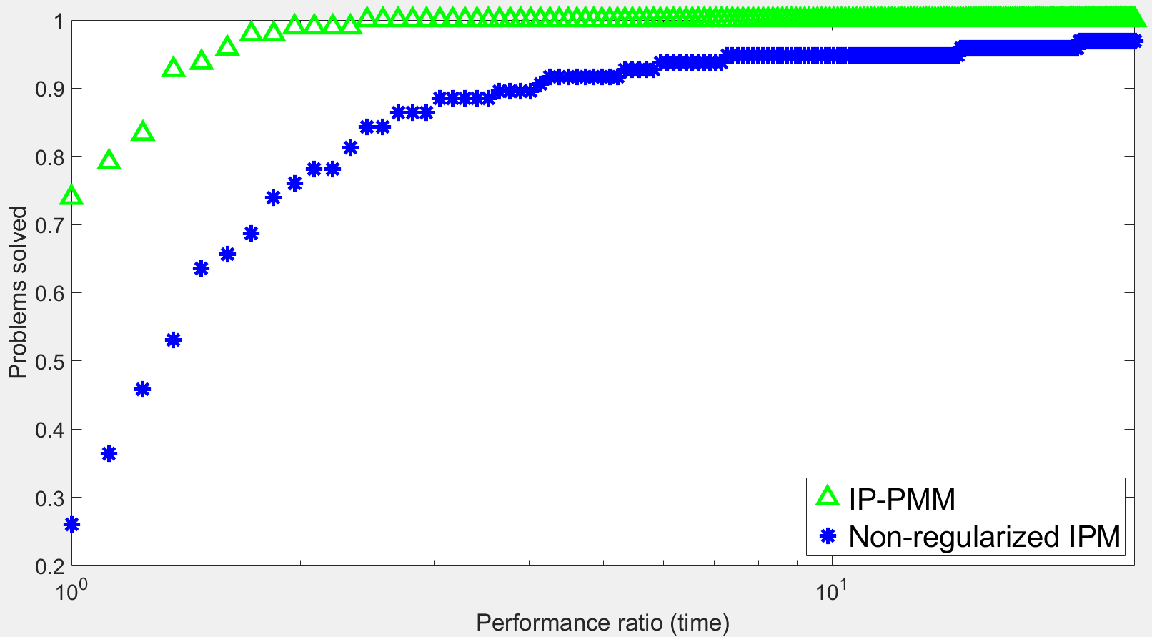
(a) Performance profile - time.

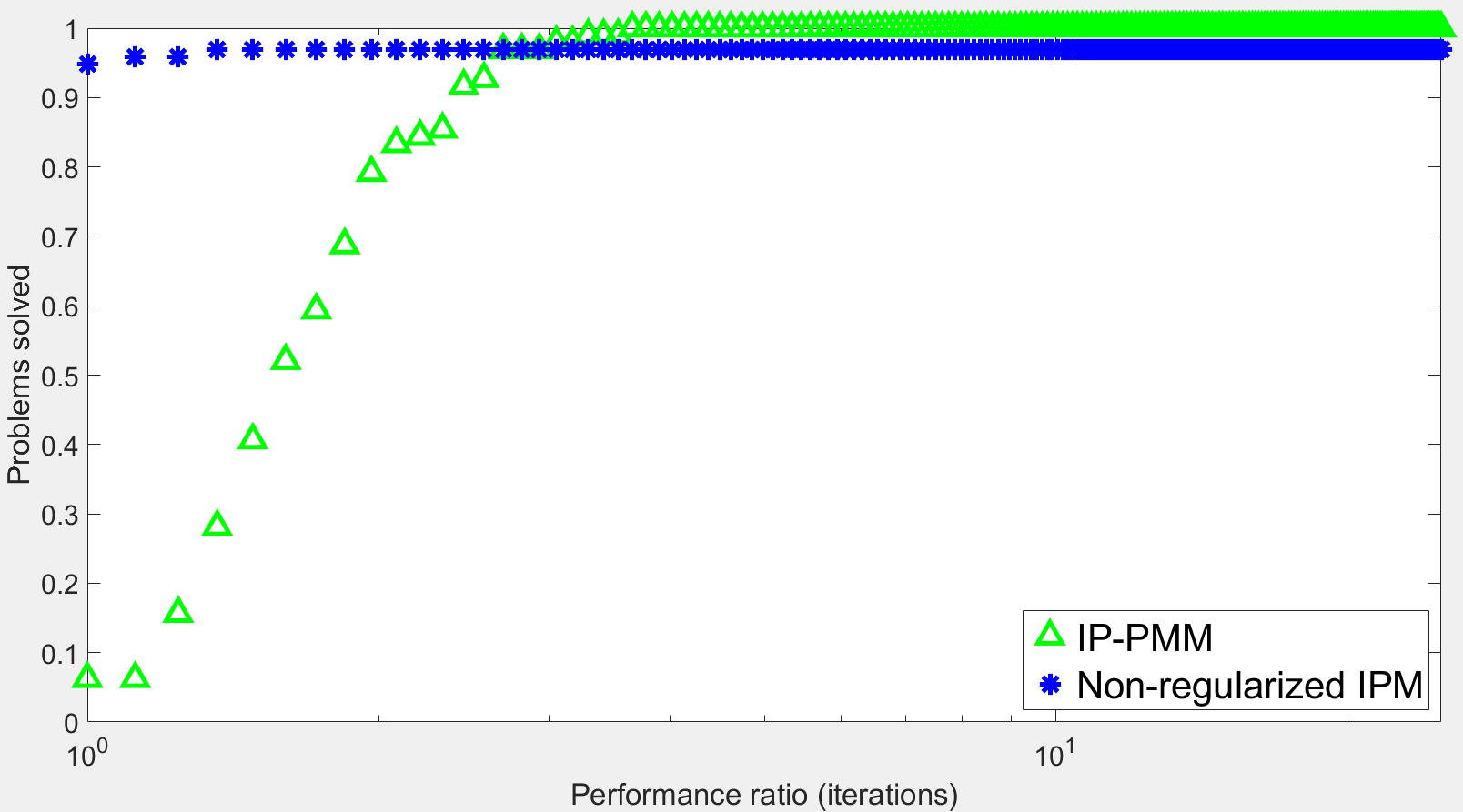
(b) Performance profile - iterations.

Infeasible Problems

In order to assess the accuracy of the proposed infeasibility detection criteria, we attempt to solve 28 infeasible problems, coming from the Netlib infeasible collection ([26], see also Infeasible Problems). For 22 out of the 28 problems, the method was able to recognize that the problem under consideration is infeasible, and exit before the maximum number of iterations was reached. There were 4 problems, for which the method terminated after reaching the maximum number of iterations. For 1 problem the method was terminated early due to numerical instability. Finally, there was one problem for which the method converged to the least squares solution, which satisfied the optimality conditions for a tolerance of $10^{-6}$. Overall, IP-PMM run all 28 infeasible problems in 34 seconds (and a total of 1,813 IPM iterations). The proposed infeasibility detection mechanism had a 78% rate of success over the infeasible test set, while no feasible problem was misclassified as infeasible. A more accurate infeasibility detection mechanism could be possible, however, the proposed approach is easy to implement and cheap from the computational point of view. Nevertheless, the interested reader is referred to [4, 25] and the references therein, for various other infeasibility detection methods.

Quadratic Programming Problems

Next, we present the comparison of the two methods over the Maros–Mészáros test set ([21]), which is comprised of 122 convex quadratic programming problems. Notice that in the previous experiments, we used the pre-solved version of the collection. However, we do not have a pre-solved version of this test set available. Since the focus of the paper is not on the pre-solve phase of convex problems, we present the comparison of the two methods over the set, without applying any pre-processing. As a consequence, non-regularized IPM fails to solve 27 out of the total 122 problems. However, only 11 out of 27 failed due to rank deficiency. The remaining 16 failures occurred due to numerical instability. On the contrary, IP-PMM solved the whole set successfully in 127 seconds (and a total of 3,014 iterations). As before, the required tolerance was set to $10^{-6}$.

In Table 2, we collect statistics from the runs of the two methods over some medium scale instances of the Maros–Mészáros collection.

Table 2: Medium-Scale Maros–Mészáros Problems

Name	$\bm{nnz(A)}$	$\bm{nnz(Q)}$	IP-PMM		IPM
			Time (s)	IP-Iter.	Time (s)	IP-Iter.
AUG2DCQP	$40,000$	$40,400$	4.70	83	7.21	111
CVXQP1L	$14,998$	$69,968$	25.54	38	$\dagger$	$\dagger$
CVXQP3L	$22,497$	$69,968$	45.69	59	$\dagger$	$\dagger$
LISWET1	$30,000$	$10,002$	1.07	30	1.86	40
POWELL20	$20,000$	$10,000$	1.26	30	1.61	25
QSHIP12L	$16,170$	$122,433$	0.91	23	$\dagger$	$\dagger$
STCQP1	$13,338$	$49,109$	0.38	16	6.89	13

In order to summarize the comparison of the two methods, we include Figure 2, which contains the performance profiles, over the Maros–Mészáros test set, of the two methods. IP-PMM is represented by the green line (consisted of triangles), while non-regularized IPM by the blue line (consisted of stars). In Figure 2(a), we present the performance profile with respect to time required for convergence, while in Figure 2(b), the performance profile with respect to the number of iterations.

Figure 2: Performance profiles over the Maros–Mészáros test set.

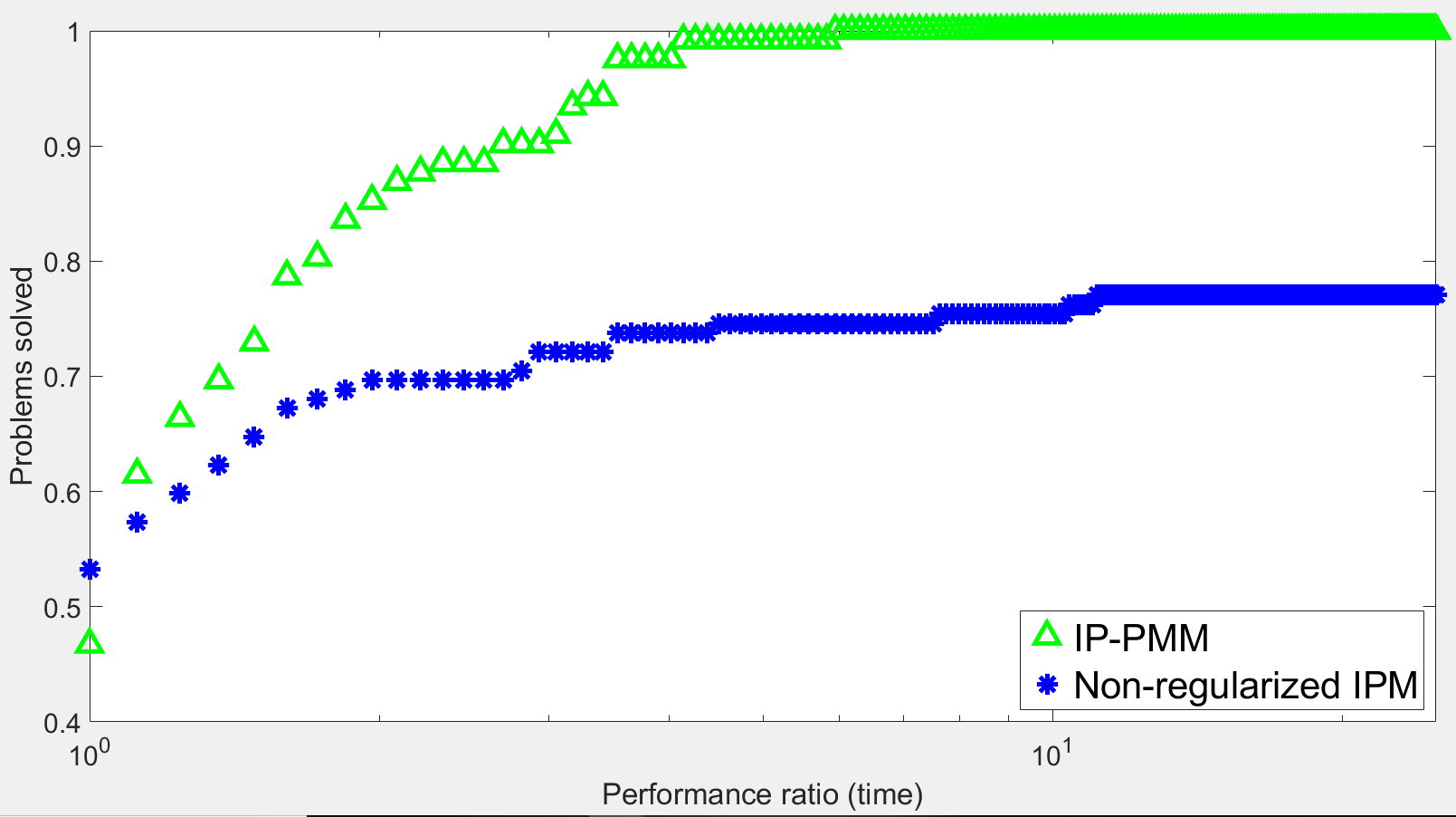
(a) Performance profile - time.

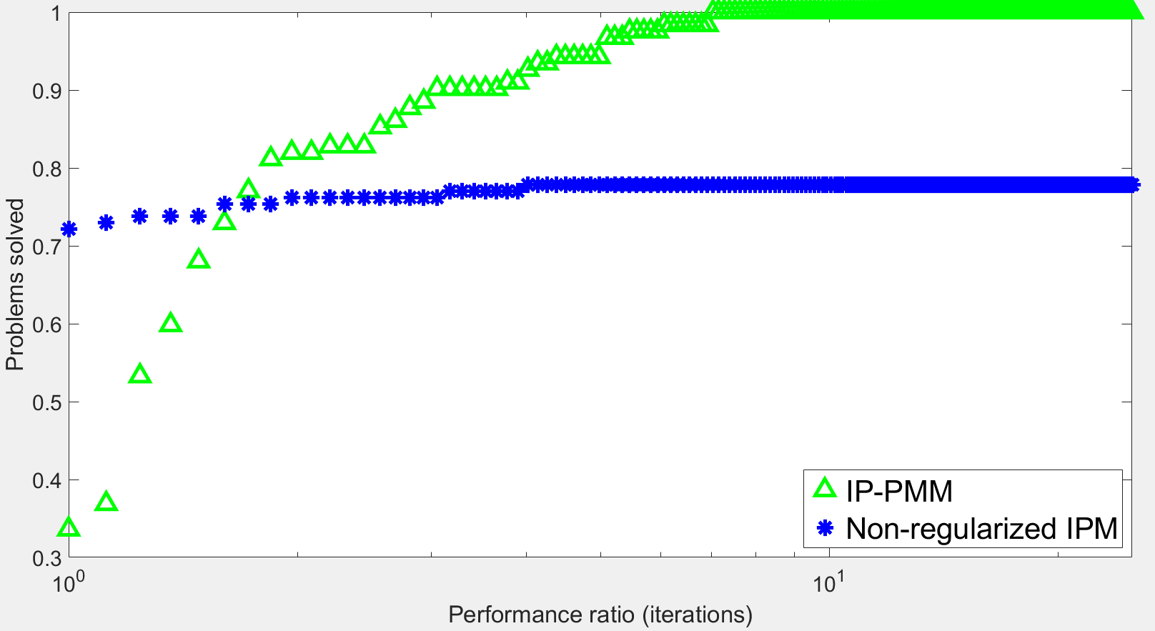
(b) Performance profile - iterations.

Similar remarks can be made here, as those given when summarizing the linear programming experiments. One can readily observe the importance of the stability introduced by the regularization. On the other hand, the overhead in terms of number of iterations that is introduced due to regularization, is acceptable due to the acceleration of the factorization (since we are guaranteed to have a quasi-definite augmented system).

Verification of the Theory

We have already presented the benefits of using regularization in interior point methods. A question arises, as to whether a regularized IPM can actually find an exact solution of the problem under consideration. Theoretically, we have proven this to be the case. However, in practice one is not allowed to decrease the regularization parameters indefinitely, since ill-conditioning will become a problem. Based on the theory of augmented Lagrangian methods, one knows that sufficiently small regularization parameters suffice for exactness (see [6], among others). In what follows, we provide a “table of robustness” of IP-PMM. We run the method over the Netlib and the Maros-Mészáros collections, for decreasing values of the required tolerance and report the number of problems that converged.

Table 3: Table of Robustness

Test Set	Tolerance	Problems Converged
Netlib (non-presolved)	$10^{-6}$	96/96
”	$10^{-8}$	95/96
”	$10^{-10}$	94/96
Netlib (presolved)	$10^{-6}$	96/96
”	$10^{-8}$	94/96
”	$10^{-10}$	94/96
Maros-Mészáros	$10^{-6}$	122/122
”	$10^{-8}$	121/122
”	$10^{-10}$	112/122

One can observe from Table 3 that IP-PMM is sufficiently robust. Even in the case where a 10 digit accurate solution is required, the method is able to maintain a success rate larger than 91%.

Large Scale Problems

All of our previous experiments were conducted on small to medium scale linear and convex quadratic programming problems. We have showed (both theoretically and practically) that the proposed method is reliable. However, it is worth mentioning the limitations of the current approach. Since we employ exact factorization during the iterations of the IPM, we expect that the method will be limited in terms of the size of the problems it can solve. The main bottleneck arises from the factorization, which does not scale well in terms of processing time and memory requirements. In order to explore the limitations, in Table 4 we provide the statistics of the runs of the method over a small set of large scale problems. It contains the number of non-zeros of the constraint matrices, as well as the time needed to solve the problem. The tolerance used in these experiments was $10^{-6}$.

Table 4: Large-Scale Problems

Name	Collection	$\bm{nnz(A)}$	time (s)	Status
fome21	Mittelmann	751,365	567.26	opt
pds-10	Mittelmann	250,307	40.00	opt
pds-30	Mittelmann	564,988	447.81	opt
pds-60	Mittelmann	1,320,986	2,265.39	opt
pds-100	Mittelmann	1,953,757	-	no memory
rail582	Mittelmann	402,290	91.10	opt
cre-b	Kennington	347,742	24.48	opt
cre-d	Kennington	323,287	23.49	opt
stocfor3	Kennington	72,721	4.56	opt
ken-18	Kennington	667,569	77.94	opt
osa-30	Kennington	604,488	1723.96	opt
nug-20	QAPLIB	304,800	386.12	opt
nug-30	QAPLIB	1,567,800	-	no memory

From Table 4, it can be observed that as the dimension of the problem grows, the time to convergence is significantly increased. This increase in time is disproportionate for some problems. The reason for that, is that the required memory could exceed the available RAM, in which case the swap-file is activated. Access to the swap memory is extremely slow and hence the time could potentially increase disproportionately. On the other hand, we retrieve two failures due to lack of available memory. The previous issues could potentially be addressed by the use of iterative methods. Such methods, embedded in the IP-PMM framework, could significantly relax the memory as well as the processing requirements, at the expense of providing inexact directions. Combining IP-PMM (which is stable and reliable) with such an inexact scheme (which could accelerate the IPM iterations) seems to be a viable and competitive alternative and will be addressed in a future work.

6 Conclusions

In this paper, we present an algorithm suitable for solving convex quadratic programs. It arises from the combination of an infeasible interior point method with the proximal method of multipliers (IP-PMM). The method is interpreted as a primal-dual regularized IPM, and we prove that it is guaranteed to converge in a polynomial number of iterations, under standard assumptions. As the algorithm relies only on one penalty parameter, we use the well-known theory of IPMs to tune it. In particular, we treat this penalty as a barrier parameter, and hence the method is well-behaved independently of the problem under consideration. Additionally, we derive a necessary condition for infeasibility and use it to construct an infeasibility detection mechanism. The algorithm is implemented, and the reliability of the method is demonstrated. At the expense of some extra iterations, regularization improves the numerical properties of the interior point iterations. The increase in the number of iterations is benign, since factorization efficiency as well as stability is gained. Not only the method remains efficient, but it outperforms a similar non-regularized IPM scheme.

We observe the limitations of the current approach, due to the cost of factorization, and it is expected that embedding iterative methods in the current scheme might further improve the scalability of the algorithm at the expense of inexact directions. Since the reliability of IP-PMM is demonstrated, it only seems reasonable to allow for approximate Newton directions and still expect fast convergence. Hence, a future goal is to extend the theory as well as the implementation, in order to allow the use of iterative methods for solving the Newton system.

References

- [1] A. Altman and J. Gondzio. Regularized Symmetric Indefinite Systems in Interior Point Methods for Linear and Quadratic Optimization. Optim. Meth. and Soft., Vol. 11 & 12 : 275–302, 1999.
- [2] P. Armand and J. Benoist. Uniform Boundedness of the Inverse of a Jacobian Matrix Arising in Regularized Interior-Point Methods. Math. Prog., Vol. 137 (No. 1&2): 587–592, 2013.
- [3] P. Armand and R. Omheni. A Mixed Logarithmic Barrier-Augmented Lagrangian Method for Nonlinear Optimization. J. Optim. Theory and Appl., Vol. 173 : 523–547, 2017.
- [4] P. Armand and N. N. Tran. Rapid Infeasibility Detection in a Mixed Logarithmic Barrier-Augmented Lagrangian Method for Nonlinear Optimization. Optim. Meth. and Soft., Vol. 34 (No. 5): 991–1013, 2019.
- [5] S. Arreckx and D. Orban. A Regularized Factorization-Free Method for Equality-Constrained Optimization. SIAM J. Optim., Vol. 28 (No. 2): 1613–1639, 2018.
- [6] P. D. Bertsekas. Constrained Optimization and Lagrange Multiplier Methods. Athena Scientific, 1996.
- [7] P. D. Bertsekas, A. Nedic, and E. Ozdaglar. Convex Analysis and Optimization. Athena Scientific, 2003.
- [8] P. D. Bertsekas and N. J. Tsitsiklis. Parallel and Distributed Computation: Numerical Methods. Athena Scientific, 1997.
- [9] Y. Censor and A. Zenios. Proximal Minimization Algorithm with D-Functions. J. of Optim. Theory and Appl., Vol. 73 (No. 3): 451–464, 1992.
- [10] D. E. Dolan and J. J. Moré. Benchmarking Optimization Software with Performance Profiles. Math. Prog. Ser. A., Vol. 91 : 201–213, 2002.
- [11] J. Eckstein. Nonlinear Proximal Point Algorithms Using Bregman Functions, with Applications to Convex Programming. Math. of Operational Research, Vol. 18 (No. 1), 1993.
- [12] M. P. Friedlander and D. Orban. A Primal-Dual Regularized Interior-Point Method for Convex Quadratic Programs. Math. Prog. Comp., Vol. 4 (No. 1): 71–107, 2012.
- [13] O. Gler. New Proximal Point Algorithms for Convex Minimization. SIAM J. Optim., Vol. 2 (No. 4): 649–664, 1992.
- [14] E. P. Gill and P. D. Robinson. A Primal-Dual Augmented Lagrangian. Comp. Optim. Appl., Vol. 51 : 1–25, 2012.
- [15] J. Gondzio. Multiple Centrality Corrections in a Primal-Dual Method for Linear Programming. Comp. Optim. and Appl., Vol. 6 : 137–156, 1996.
- [16] J. Gondzio. Interior Point Methods 25 Years Later. European J. of Operational Research, Vol. 218 (No. 3): 587–601, 2013.
- [17] M. R. Hestenes. Multiplier and Gradient Methods. J. of Optim. Theory and Appl., (No. 4):303–320, 1969.
- [18] A. N. Iusem. Some Properties of Generalized Proximal Point Methods for Quadratic and Linear Programming. J. of Optim. Theory and Appl., Vol. 85 (No. 3): 593–612, 1995.
- [19] M. Kojima, N. Megiddo, and S. Mizuno. A Primal-Dual Infeasible-Interior-Point Algorithm for Linear Programming. Math. Prog., Vol. 61 : 263–280, 1993.
- [20] G. Lan and R. D. C. Monteiro. Iteration-Complexity of First-Order Augmented Lagrangian Methods for Convex Programming. Math. Prog., Vol. 155 (No. 1-2): 511–547, 2016.
- [21] I. Maros and C. Mészáros. A Repository of Convex Quadratic Programming Problems. Optim. Meth. and Soft., Vol. 11 & 12 : 671–681, 1999.
- [22] S. Mehrotra. On the Implementation of a Primal-Dual Interior-Point Method. SIAM J. Optim., Vol. 2 (No. 4): 575–601, 1992.
- [23] S. Mizuno and F. Jarre. Global and Polynomial-Time Convergence of an Infeasible-Interior-Point Algorithm using Inexact Computation. Math. Prog., Vol. 84 : 105–122, 1999.
- [24] Y. Nesterov and A. Nemirovski. Interior-Point Polynomial Algorithms in Convex Programming. SIAM, 1993.
- [25] Y. Nesterov, M. J. Todd, and Y. Ye. Infeasible-Start Primal-Dual Methods and Infeasibility Detectors for Nonlinear Programming Problems. Math. Prog., Vol. 82 (No. 2): 227–267, 1999.
- [26] Netlib. http://netlib.org/lp, 2011.
- [27] N. Parikh and S. Boyd. Proximal Algorithms. Foundations and Trends in Optim., Vol. 3 (No. 1): 123–231, 2014.
- [28] S. Pougkakiotis and J. Gondzio. Dynamic Non-diagonal Regularization in Interior Point Methods for Linear and Convex Quadratic Programming. J. of Optim. Theory and Appl., Vol. 181 (No. 3): 905–945, 2019.
- [29] M. J. D. Powell. A Method for Nonlinear Constraints in Minimization Problems. Optim., (No. 4): 283–298, 1969.
- [30] R. T. Rockafellar. Augmented Lagrangians and Applications of the Proximal Point Algorithm in Convex Programming. Math. of Operations Research, Vol. 1 (No. 2): 97–116, 1976.
- [31] R. T. Rockafellar. Monotone Operators and the Proximal Point Algorithm. SIAM J. Control and Optim., Vol. 14 (No. 5), 1976.
- [32] R. T. Rockafellar. Convex Analysis. Princeton University Press, 1996.
- [33] R. Vanderbei. Symmetric Quasidefinite Matrices. SIAM J. Optim., Vol. 5 (No. 1): 100–113, 1995.
- [34] Y. Wang and P. Fei. An Infeasible Mizuno-Todd-Ye Type Algorithm for Convex Quadratic Programming with Polynomial Complexity. Numer. Funct. Anal. and Optim., Vol. 28 (No. 3-4): 487–502, 2007.
- [35] S. J. Wright. Primal-Dual Interior Point Methods. SIAM, 1997.
- [36] Y. Zhang. On the Convergence of a Class of Infeasible Interior-Point Methods for the Horizontal Linear Complementarity Problem. SIAM J. Optim., Vol. 4 (No. 1): 208–227, 1994.
- [37] G. Zhou, K. C. Toh, and G. Zhao. Convergence Analysis of an Infeasible Interior Point Algorithm Based on a Regularized Central Path for Linear Complementarity Problems. Comp. Optim. Appl., Vol. 27 (No. 3): 269–283, 2004.